Article

Influencing Factor Analysis of Vegetation Spatio-Temporal Variability in the Beijing–Tianjin–Hebei Region Based on Interpretable Machine Learning

1
Hebei University of Engineering, Handan 056038, China
2
Zunhua Emergency Management Bureau, Zunhua 064299, China
*
Author to whom correspondence should be addressed.
Forests 2025, 16(12), 1873; https://doi.org/10.3390/f16121873
Submission received: 13 November 2025 / Revised: 11 December 2025 / Accepted: 15 December 2025 / Published: 18 December 2025

Abstract

To address the insufficient quantitative understanding of vegetation driving mechanisms across spatio-temporal scales, this study integrated multi-source data and machine learning methods to simulate and analyze Normalized Difference Vegetation Index (NDVI) changes in the Beijing–Tianjin–Hebei (BTH) region over the past two decades. Using the SHapley Additive exPlanations (SHAP) method, we identified the most important predictors of climate and human activities in the XGBoost model and quantified their spatial contributions. We further analyzed the spatio-temporal variation of the main predictors across different land use types The main findings were as follows: (1) The XGBoost model achieved excellent performance (R2 > 0.96, MEA < 0.02, RMSE < 0.027) on the datasets from 2000 to 2020, outperforming random forest (RF), support vector machines (SVM), and K-nearest neighbors (KNN) in prediction accuracy. (2) Vegetation showed an overall improving trend, with areas exhibiting significant improvement accounting for 47.96% of the total region. Precipitation, temperature, and human activities were identified as the most significant predictors of NDVI. Their relative importance varied over time, and NDVI responses to these factors exhibited clear spatial heterogeneity. (3) Primary predictors differed by land use type: NDVI in cropland and grassland was mainly driven by precipitation, forest NDVI by temperature, and urban/built-up areas by human activities. This study developed an analytical framework integrating nonlinearity and spatial heterogeneity, achieving a quantitative “overall-categorical” analysis of the important predictors behind NDVI changes. The approach provided a novel methodological reference for attributing vegetation dynamics. The findings contributed to the implementation of classified regulation in the BTH region, promoting the transition of human activities toward ecological restoration.

1. Introduction

Vegetation, as a key component of the Earth’s geographical environment, plays fundamental functional roles within the biosphere and ecosystems. Vegetation changes at regional and global scales significantly impact energy and biogeochemical cycles, as well as climate dynamics [1,2,3]. Both natural and anthropogenic factors drive vegetation growth. These changes can alter land surface properties, ultimately affecting climate regulation and overall ecosystem stability [4,5,6]. The rapid development of the BTH region is accompanied by significant ecological environment pressures. The “BTH Coordinated Development Plan Outline” identifies ecological environment protection as a key focus for regional collaborative development and an area requiring urgent improvement. In response, the government has implemented a series of ecological restoration projects to balance social development and ecological protection needs, such as the Three-North Shelterbelt Program, the Grain for Green, the Beijing-Tianjin Sandstorm Source Control Program, and the Taihang Mountains Afforestation Project. Vegetation change serves as a crucial indicator for assessing regional ecological health. Therefore, assessing vegetation dynamics and their driving factors in the BTH region offers valuable insights for optimizing ecological conservation strategies and promoting harmonious coexistence between human activities and the natural environment.
Numerous scholars have utilized NDVI to analyze vegetation dynamics at global or regional scales [7,8,9]. They further investigated its influencing factors from perspectives such as climate (temperature, precipitation) [10,11], topography (elevation, slope, aspect) [12,13], moisture conditions (soil moisture, vapor pressure deficit) [14,15], and anthropogenic activities (population density, land use type, nighttime light) [16,17,18]. These studies have found that temperature and precipitation were the primary influencing factors, though their effects vary significantly across regions [19]. Additionally, research has shown that vegetation growth in arid regions is strongly constrained by soil moisture and vapor pressure deficit [20,21]; furthermore, as human society continues to develop, vegetation dynamics are increasingly influenced by human activities, to the extent that they even alter the growth environment and distribution patterns of vegetation on regional scales [22]. Previous studies have widely adopted statistical analysis methods to systematically assess the impact of factors such as climate and human activities on vegetation dynamics [23,24,25]. However, vegetation dynamics is influenced by multiple factors, making it difficult for these methods to accurately quantify the individual impact. For instance, in applications of Geographically Weighted Regression (GWR), multicollinearity can lead to the local repetition of similar factors. This may artificially inflate the explanatory power of certain variables, thereby compromising the accuracy of the analysis regarding factor influences [10,26]. In contrast, despite its advantages in handling non-linear relationships and quantifying individual variable contributions, the Geodetector method is limited to providing statistical measures of factor importance. It cannot reveal the spatial direction or magnitude of the influencing factors [27,28].
In recent years, machine learning methods such as KNN, SVR, RF, and XGBoost have been widely utilized to explore the impacts of climate and human activities on vegetation [29,30]. KNN is a non-parametric supervised learning algorithm that makes predictions based on samples within a local neighborhood. Although intuitive, its computational complexity increases with the sample size. SVR employs kernel functions to map input variables into high-dimensional feature spaces and seeks an optimal hyperplane, offering good robustness for small-sample nonlinear data and outliers [31]. RF adopts a Bagging ensemble strategy by constructing multiple decision trees and aggregating their results, effectively avoiding issues such as variable collinearity and overfitting [32]. XGBoost is an advanced implementation of gradient boosting decision trees in ensemble learning [33]. It optimizes the loss function through second-order Taylor expansion and incorporates regularization and tree-structure control mechanisms, demonstrating outstanding performance in prediction accuracy, computational efficiency, and generalization capability. These methods collectively form a multi-level methodological system ranging from simple to complex and from linear to nonlinear. They are often criticized as “black-box” models, and although some algorithms such as RF and XGBoost can effectively output the relative importance of various influencing factors on vegetation growth, they cannot reveal the spatio-temporal patterns of how primary factors influence vegetation changes. Moreover, the primary factors affecting vegetation vary significantly across regions, time periods, and land use types, exhibiting considerable heterogeneity. Consequently, evaluating factor importance and quantifying their independent spatio-temporal impacts remain a significant challenge. The SHAP interpretable methods addresses this limitation by combining machine learning’s powerful data-fitting capability with transparent interpretation of results [34]. Python extension packages have been developed that employ SHAP to interpret outputs from a variety of machine learning models [35]. These packages seamlessly integrate XGBoost and various Scikit-Learn models into the SHAP interface, simplifying SHAP-based interpretation of XGBoost results. With the growing integration of machine learning and SHAP interpretability, the XGBoost-SHAP framework has emerged as a promising approach for the robust quantification of factor contributions. For instance, interpretable machine learning had been employed to evaluate the combined effects of temperature, precipitation, soil moisture, and land use changes on vegetation dynamics in the Yellow River Basin [15]. Likewise, the XGBoost-SHAP framework was applied to examine climatic influences on net primary production in the Amazon rainforest, revealing distinct spatial variations in the dominant driving factors [36]. While the SHAP method is built upon the assumption of feature independence that may lead to less reliable results when handling correlated variables, it demonstrates extensive applicability in understanding the influencing factors of Earth science phenomena [37,38,39]. Not only can it quantify the overall importance of influencing factors, but it can also reveal the distribution and degree of influence across spatial units, overcoming the limitation of traditional methods that only provide global feature importance [40,41].
To support ecological environment monitoring, several researchers have investigated NDVI changes and their influencing factors in the BTH region using remote sensing data. For instance, Yan et al. had further examined how vegetation responds to climatic and non-climatic drivers across different seasons, topographic conditions, and vegetation types [42]. Another study employed random forests to disaggregate the relative contributions of climate and anthropogenic activities to vegetation dynamics [43]. However, these studies have yet to fully account for the spatial heterogeneity of these influencing factors. Moreover, research on NDVI changes across different land use types remains insufficiently detailed.
To address the inadequate analysis of the spatio-temporal mechanisms and influencing factors of NDVI changes across different land use types, this study introduces the XGBoost-SHAP method. Based on time-series data of the BTH region from 2000 to 2020, we conducted high-precision NDVI simulation and quantitative attribution analysis of influencing factors. This study aimed to (1) develop an optimal vegetation NDVI simulation model and identify the primary factors influencing NDVI dynamics across different temporal periods; (2) reveal the spatial heterogeneity and quantitative impacts of these dominant factors; and (3) characterize differences in factor importance among land use types. The advantages of this study are mainly reflected in two aspects. First, the method effectively captures the nonlinear influences of various factors, quantitatively interpreting their direction, strength, and spatial heterogeneity. Second, it systematically reveals the primary influencing factors and their differential mechanisms behind NDVI changes across different land use types, thereby advancing understanding from an overall to a categorized perspective. This study can provide a decision-making basis for implementing differentiated ecological restoration and land management in the BTH region.

2. Materials and Methods

2.1. Study Area

Located in the northern part of the North China Plain, the BTH region comprises two municipalities (Beijing and Tianjin) and eleven prefecture-level cities in Hebei Province (Figure 1a). The topography generally exhibits a stepwise decline from northern mountainous areas to southern plains. The total area is approximately 217,000 km2, with a population of about 110 million. According to 2020 land use data (Figure 1b), the area proportions of the main land cover types are as follows: cropland (43.8%), forest (21.6%), grassland (14.9%), and urban and built-up areas (14.5%). The region experiences a temperate monsoon climate, characterized by cold, dry winters and hot, humid summers. The annual average temperature ranges from 10.4 °C to 11.9 °C, and the annual average precipitation varies between 375.5 mm and 684.7 mm. Against the backdrop of global climate change, extreme weather events have become more frequent. The vegetation types are diverse, and in recent years, the overall trend has shown a complex pattern of “general improvement with localized degradation,” with significant anthropogenic driving forces. This region lies within the ecologically fragile zone of North China, exhibiting high sensitivity to climate change. Simultaneously, it is influenced by the dual pressures of intensive urbanization and large-scale ecological engineering projects, representing a typical highly coupled natural–social system.

2.2. Data

We utilized NDVI data obtained from the MODIS MOD13Q1 product (https://search.earthdata.nasa.gov/search, accessed on 16 February 2024), with a spatial resolution of 250 m and a temporal resolution of 16 days. High-quality NDVI data during the vegetation growing season (April to October) from 2000 to 2020 were selected. The data utilized the VI_Quality band for product quality assessment and had undergone atmospheric correction, effectively removing the direct interference from water vapor, aerosols, clouds, and shadows. To minimize noise caused by atmospheric interference, cloud cover, and solar zenith angle variations, the Maximum Value Composite (MVC) method was employed to extract the maximum pixel values and reconstruct annual NDVI datasets. The effects of low-value noise were eliminated, thereby obtaining the interannual NDVI time-series data for the BTH region from 2000 to 2020.
To investigate the relationship between NDVI and its predictors, we selected 14 representative variables across five categories (climate, terrain, hydrology, soil conditions, and human activities) based on established ecological principles, data availability, and previous vegetation studies [12,14,44]. The complete list of factors and their data sources are presented in Table 1.
The temperature and precipitation data were sourced from the National Earth System Science Data Center (http://www.geodata.cn/, accessed on 22 March 2024), specifically the 1 km resolution monthly dataset for China, which has been updated to 2022 [45]. DEM data was acquired from the United States Geological Survey (https://www.usgs.gov/, accessed on 3 March 2024) at 90 m spatial resolution. The global high-resolution land surface assimilation dataset developed by the Famine Early Warning Systems Network Land Data Assimilation System (FLDAS) (https://disc.gsfc.nasa.gov/datasets/, accessed on 9 May 2024), using monthly global soil moisture data at 0.1° × 0.1° resolution across four depth layers: 0–10 cm, 10–40 cm, 40–100 cm, and 100–200 cm [46]. The Vapor Pressure Deficit (VPD) refers to the difference between the saturation vapor pressure (es) and the actual vapor pressure (ea) in the air at a given temperature, indicating the degree of air dryness. VPD is calculated according to the following equation [47,48]:
e s = 0.611 × exp 17.27 × T a T a + 237.3
e a = R H 100 * e s
V P D = e s e a = e s * ( 1 R H 100 )
where VPD (kPa) denotes Vapor Pressure Deficit, es denotes the saturation vapor pressure, and ea represents the actual vapor pressure, T a (°C) is air temperature, R H (%) is relative humidity.
We acquired anthropogenic driving factor data from multiple sources, with land use, population density, and clay ratio data obtained from the Chinese Academy of Sciences Resource and Environmental Science Data Center (http://www.resdc.cn/, accessed on 2 April 2024). These land use data were filtered and divided into cropland, natural vegetation, and impervious surface, and their proportional areal coverage within each unit area was calculated, with a spatial resolution of 30 m. The spatial resolution of population density and clay proportion is 1 km, with a temporal resolution of 5 years. Additionally, we incorporated the “NPP-VIIRS-like NTL Data” dataset from Chen et al., which represents a significant advancement in cross-sensor calibration for nighttime light remote sensing [49]. This dataset is a unified product resulting from the systematic integration of DMSP/OLS and VIIRS nighttime light data, with a spatial resolution of 1 km and a temporal resolution of 1 year. It is obtained from the Harvard Dataverse (https://dataverse.harvard.edu/, accessed on 10 April 2024). For vegetation impact factor analysis, we systematically processed data from five representative years (2000, 2005, 2010, 2015, and 2020). Following preprocessing steps such as image stitching and outlier removal, all datasets were uniformly projected into the WGS84 coordinate system and resampled to 1 km spatial resolution using bilinear interpolation to meet model requirements by using GIS software. Using the BTH regional administrative boundaries as our spatial framework, we performed geographic clipping operations. Subsequently, grid cell information was iteratively extracted into point information and saved in plain text format. The original data were filtered according to the applicable conditions of all variables, resulting in approximately 175,000 samples per phase. The study utilized both annual and monthly data. To focus on interannual variations, monthly data such as NDVI and meteorological factors during the growing season were annualized by taking the maximum or mean values. This approach was widely employed to reveal interannual trends and maintain scale consistency with other annual data, thereby constructing a unified analytical framework [32]. It should be noted that analyses based on annual scales smooth out short-term extreme fluctuations, which may affect the magnitude and interpretation of SHAP values for model predictor variables.

2.3. Methods

This study focused on investigating the spatio-temporal variations of NDVI in the BTH region and quantitatively interpreting its influencing factors. Independent models were constructed using NDVI data and its influencing factors for each period, and the performance of four models in simulating NDVI was compared to identify the optimal machine learning model. Based on this, interpretability method was applied to deeply analyze the spatio-temporal variation characteristics of factors influencing NDVI changes over the past two decades. The process was as follows: (1) analyzing the spatio-temporal trends of NDVI over the past two decades, both overall and across different land use types; (2) evaluating the performance of four machine learning methods in simulating NDVI and selecting the optimal model; (3) ranking the importance of influencing factors of NDVI and analyzing their spatial variations based on the SHAP values; (4) analyzing changes in the influencing factors of NDVI across different land use types. The technical flowchart is shown in Figure 2.

2.3.1. Analysis of Vegetation Change Trends

This study employed a combination of the Theil-Sen estimator and the Mann–Kendall (MK) test to analyze vegetation trends [50]. Theil-Sen estimator demonstrates strong robustness against data gaps and effectively mitigates the influence of anomalous outliers [44]. The computational formula is expressed as follows:
β = median N D V I j N D V I i j i , 2000 i < j 2020
where i , j is year of the research period; N D V I i , N D V I j is the NDVI for the year i and year j , respectively. β represents the interannual variation trend of NDVI during the study period (unit: dimensionless/year); when it is bigger than 0, it means an upward trend, whereas values below 0 indicate a downward trend.
The NDVI change trends from the previous step were subsequently subjected to significance testing using the MK method. As a non-parametric statistical approach, the MK test offers significant advantages, including being distribution-free and highly robust to outliers [51]. The process of the MK test is as follows:
S = i = 1 n 1 j = i + 1 n s g n ( N D V I j N D V I i )
s g n ( θ ) is defined as a symbolic function as follows:
s g n ( N D V I j N D V I i ) = 1 0 1 N D V I j N D V I i > 0 N D V I j N D V I i = 0 N D V I j N D V I i < 0
where N D V I i and N D V I j denote N D V I in years i and j , respectively; n is the length of the research period of 21 years; when n 8 , S follows a normal distribution and has a mean of 0. The variance is as follows:
V a r S = n ( n 1 ) ( 2 n + 5 ) 18
The formula for the normality test statistic Z is given below:
Z M K = S 1 V a r S 0 S + 1 V a r S S > 0 S = 0 S < 0
Based on the trend magnitude (β) and the statistical significance (p-value), the six types of vegetation change trends in the BTH region are as follows: highly significant degradation ( β < 0 ,   p 0.01 ), significant degradation ( β < 0 ,   0.01 p < 0.05 ), insignificant degradation ( β < 0 ,   p 0.05 ), insignificant growth ( β > 0 ,   p 0.05 ), significant growth ( β > 0 ,   0.01 p < 0.05 ), and highly significant growth ( β > 0 ,   p 0.01 ).

2.3.2. Machine Learning Model

The XGBoost model, developed by Chen and Guestrin, represents an optimized implementation of gradient boosted decision trees that delivers enhanced computational efficiency and predictive accuracy [52]. This ensemble method operates by iteratively training decision trees, where each subsequent model learns to correct the residuals of previous predictions, with the final output being the weighted sum of all tree predictions. The regression tree formula adopted is as follows:
y ^ i = φ ( Χ i ) = k = 1 K f k ( Χ i ) , f k F
where y i is the predicted value of the model; K is the number of decision trees, f k represents the k sub-model; X i represents the i input sample; F means the space of the regression tree. Based on the predicted values of the regression tree, an objective function of the model can be derived:
O bj = i = 1 n l ( y i , y ^ i ) + k = 1 K Ω ( f k )
where n is the total amount of data imported for the k regression tree; K represents all regression trees built; i = 1 n l ( y i , y ^ i ) represents the regression function based on squared error loss; k = 1 K Ω ( f k ) represents the regularization term of the objective function, the specific functions are as follows:
Ω ( f k ) = γ T + 1 2 λ ω 2
In the regression tree formulation, T denotes the number of leaf nodes; ω represents the score assigned to each leaf node; γ , λ indicate the regularization term’s penalty coefficient. The XGBoost model ensures that the contribution of each tree can be effectively utilized through its weighting method while improving model stability and generalization via regularization and feature selection [52,53].
In this study, the modeling procedure and analytical workflow were implemented using Python 3.6.6 open-source scientific computing ecosystem, including scikit-learn for machine learning, XGBoost for gradient boosting, and SHAP for model interpretation, with development conducted on the PyCharm 2023.1.2 integrated development environment.

2.3.3. Model Parameter Optimization and Evaluation

According to Chen and Guestrin, the performance of the XGBoost model requires careful parameter optimization to effectively prevent model overfitting [52]. We implemented automated hyperparameter tuning using GridSearchCV, which combines grid search with cross-validation, and selected optimal parameters for each period based on the coefficient of determination (R2) obtained through 5-fold cross-validation. Among XGBoost’s numerous parameters, the number of weak learners (n_estimators) and the learning rate (eta) are particularly critical, with eta controlling feature weight shrinkage to conservatively adjust each tree’s influence. The max_depth and min_child_weight parameters control model complexity to prevent the risk of overfitting. Through experimental testing that considers data size, model complexity, and computational constraints, we identify the optimal parameters: eta = 0.2, n_estimators = 100, gamma = 0, max_depth = 10, min_child_weight = 2, colsample_bytree = 0.8, colsample_bylevel = 1, subsample = 1, reg_lambda = 28, reg_alpha = 0.4, with random seed fixed at 42. Three standard regression metrics were employed to evaluate model performance: mean absolute error (MAE), root mean square error (RMSE), and coefficient of determination (R2). As widely adopted evaluation indicators, these metrics were calculated as follows:
M A E = 1 N i = 1 N y i T y i p
R M S E = 1 N i = 1 N y i T y i p 2
R 2 = 1 i = 1 N y i T y i p 2 i = 1 N y i T y i ¯ 2
where y i T is the true value, y i p is the predicted value, y i ¯ is the mean true values, and i is the number of observations.

2.3.4. SHapley Additive ExPlanation

The SHAP method is a game-theoretic approach to feature attribution analysis, building upon Shapley value theory [54] and local interpretability concepts [55]. Developed by Lundberg and Lee [35], this method quantitatively estimates each feature’s marginal contribution to model predictions. The Shapley value represents a feature value’s contribution to the prediction by calculating the weighted sum of its effects across all possible feature combinations, formally defined as follows [56]:
ϕ i = S N i S ! n S 1 ! n ! v S i v S
The combined Shapley values of all features collectively account for the total deviation from the model’s mean prediction, with the complete interpretable model expressed as:
g z = ϕ 0 + j = 1 M ϕ j z j
where g denotes interpretation model, z 0 , 1 M manifests whether or not the matching feature could be noticed (1 or 0), M represents the count of features selected, ϕ i R is the attribution value (Shapley value) for each feature, and ϕ 0 is the constant of the interpretation model, generated by the predicted mean of all training data. The final model prediction is calculated by summing all feature SHAP values and adjusting for the baseline prediction mean. Shapley values provide the mathematically unique solution for feature importance interpretation that satisfies both local accuracy and consistency requirements. Therefore, this study employed the Tree SHAP algorithm (shap.explainers.Tree) to interpret the output of the XGBoost algorithm, a tree-based ensemble model, and ranked the contributions of the features.

3. Results

3.1. Spatio-Temporal Changes in the NDVI

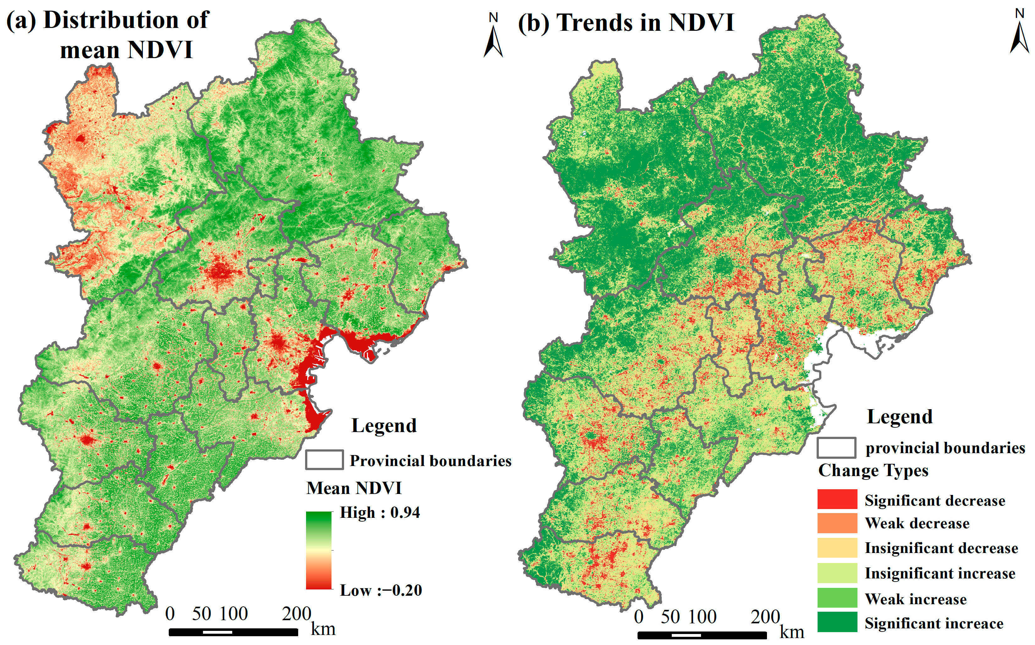
From 2000 to 2020, the BTH region exhibited relatively high vegetation coverage, along with noticeable regional variations (Figure 3a). The multi-year average NDVI reached 0.716, covering 62.31% of the total area. Spatially, lower NDVI values predominantly occurred in northern Zhangjiakou and peri-urban areas surrounding major cities. Conversely, higher NDVI values were principally concentrated in the Yanshan Mountains and southern plains. The southern plain region is part of the North China Plain, a major agricultural zone where cropland is the dominant land cover. During the study period, vegetation in the BTH region generally improved (Figure 3b). The largest proportion of the area (43.69%) showed statistically insignificant changes, mainly concentrated in the the central and southern plains. Notably, areas with significant vegetation decline (8.53%) were spatially constrained to highly urbanized zones, especially within Beijing and Tianjin. In comparison, significant vegetation increases (totaling 47.96%) were widely observed in the Taihang Mountains, as well as in Chengde and Zhangjiakou.
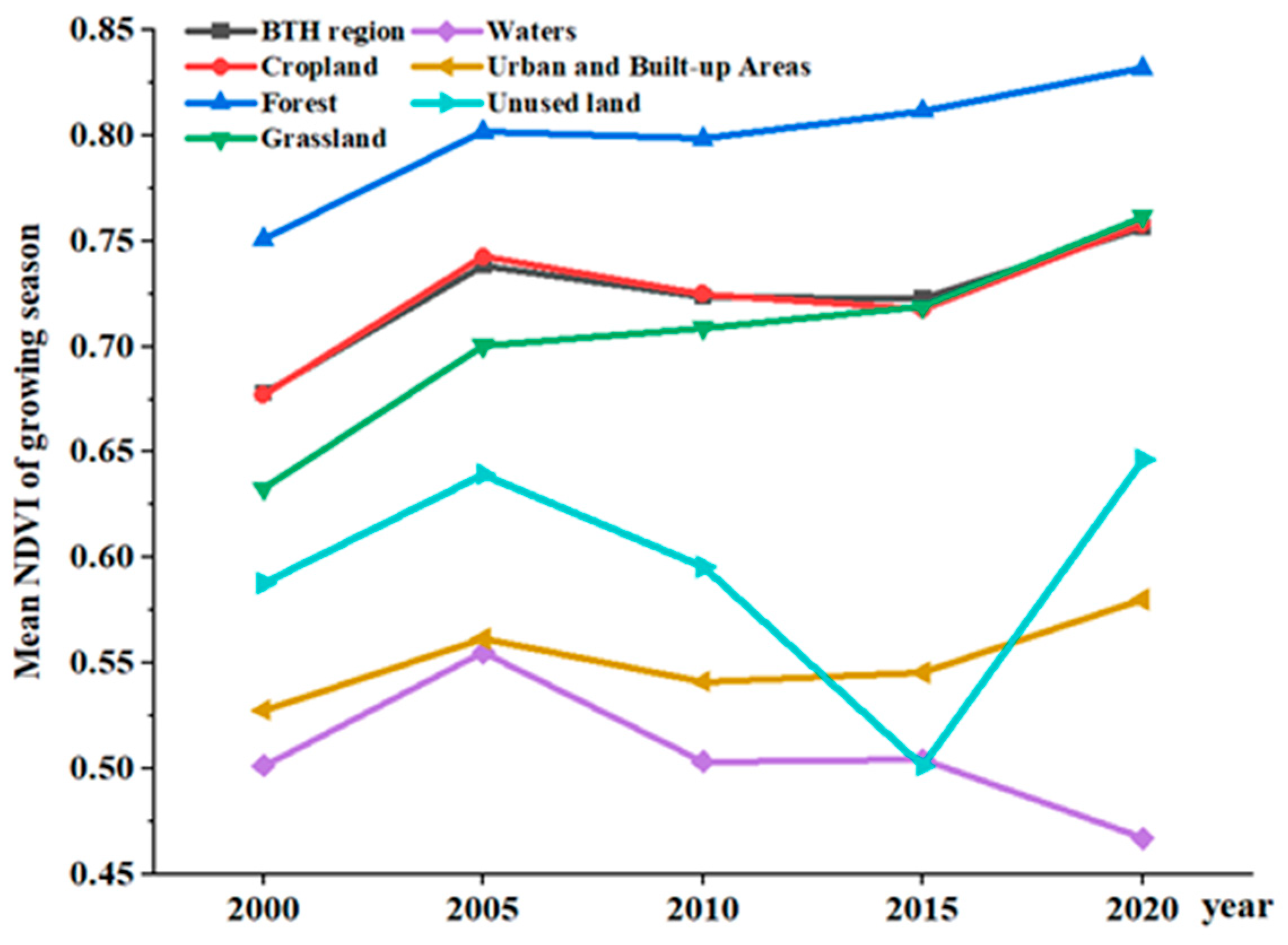
Figure 4 presented the annual mean NDVI values across different land use types in the BTH region. Cropland NDVI values (ranging 0.65–0.75) closely followed the regional average pattern. The mean NDVI of forest is the highest (>0.75) with the smallest inter-annual variability., while grassland values remained above 0.6. Urban and built-up areas showed lower vegetation coverage with mean NDVI values below 0.6, and unused land exhibited the lowest indices (all < 0.5).
Table 2 reveals the NDVI change patterns across land use types in the BTH region. Cropland vegetation experienced a net increase overall, with expansion areas surpassing degradation zones. This cropland improvement is mainly attributed to advances in agricultural technology, such as fertilizers, irrigation, and breeding, supported by substantial growth in grain output during the study period. Meanwhile, urban expansion was the primary cause of cropland reduction. Forests and grasslands showed particularly strong positive trends. Highly significant NDVI increases occurred in 65.48% of forest areas and 59.22% of grassland areas, whereas decreases were minimal (0.82% and 1.03%, respectively). These improvements directly reflected the effectiveness of regional ecological conservation policies implemented over the past two decades. In contrast, urban and built-up areas exhibited consistent vegetation decline due to intensive human activities, particularly urban expansion. Overall, forest ecosystems experienced the most extensive vegetation recovery during the study period, while urban and built-up areas showed the most pronounced degradation trends.

3.2. Model Comparison and Result Validation

For NDVI prediction across five temporal periods in the BTH region, we employed 14 influencing factors as input variables, with data randomly partitioned into training (70%) and testing (30%) sets for model development. Model performance was assessed using three established metrics: MAE, RMSE, and R2. To validate the XGBoost model’s superiority, we conducted comparative analyses with alternative machine learning approaches including RF, SVM and KNN using 2000 NDVI simulation results (Table 3). The XGBoost model demonstrated superior performance compared to the other three machine learning methods, confirming its effectiveness for vegetation NDVI simulation in the BTH region. Consequently, we employed the XGBoost model to simulate vegetation NDVI across all five study periods. Comparative analysis between predicted and observed NDVI values revealed strong correlations between input variables and NDVI (R2 > 0.96), with MAE values ranging from 0.013 to 0.020 and RMSE consistently below 0.027. The probability density plot (Figure 5) showed that the two distribution curves were essentially overlapping. Although this could not effectively test for spatial independence, it indicated consistency in the overall distribution between the predicted NDVI data and the original NDVI data. These validation results demonstrated the XGBoost model’s high predictive accuracy, establishing a reliable foundation for subsequent analysis of input variable importance.

3.3. Importance Analysis of Influencing Factors

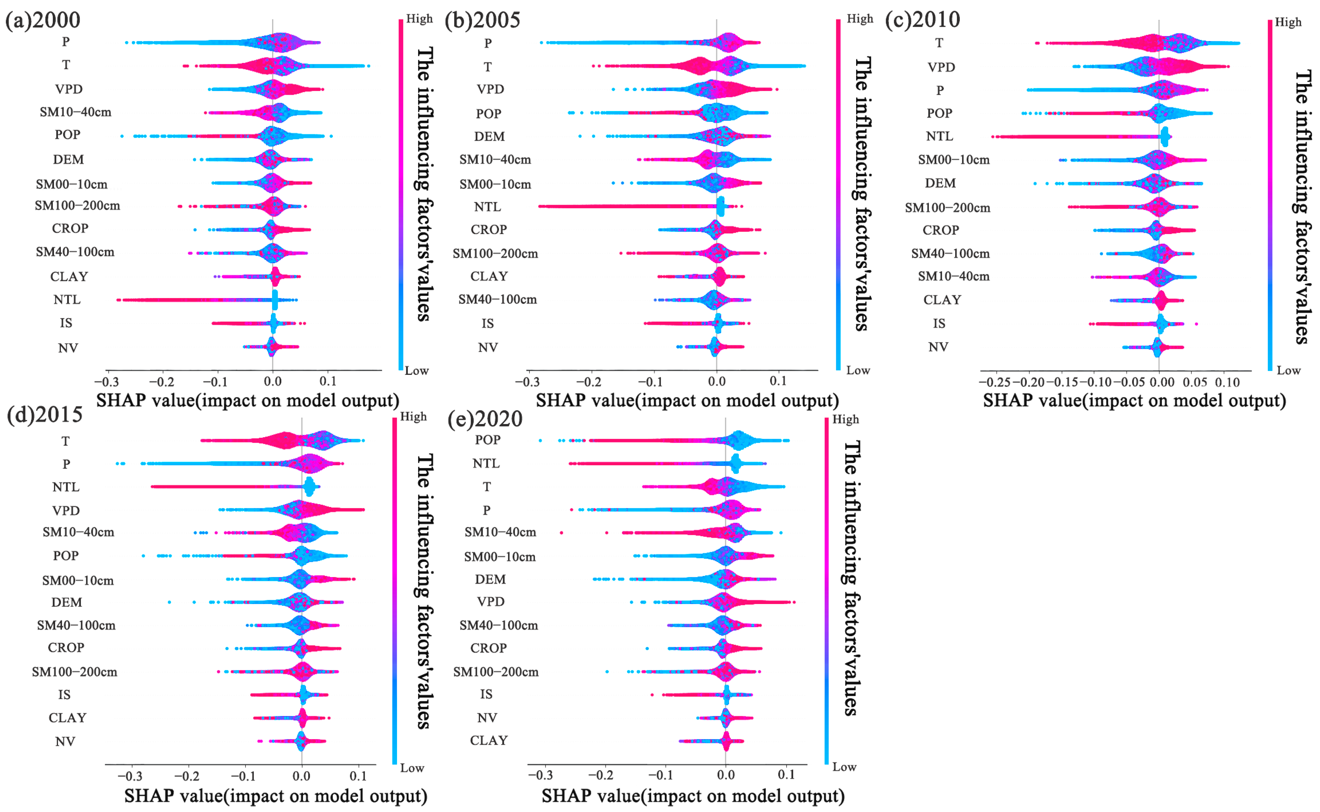
The SHAP method provides a clear framework for assessing variable importance by examining both the direction and magnitude of factors influencing NDVI, in addition to analyzing absolute values (Figure 6). On the horizontal axis, the SHAP value of each feature reflects the strength of its influence positive values indicate a favorable impact on vegetation, whereas negative values signify an adverse effect. The distribution of points shows how these influences vary across locations. Along the vertical axis, the color gradient from red to blue represents the feature value ranges, visually illustrating trends for each influencing factor. The analysis revealed that precipitation was the primary influencing factor of vegetation changes during 2000 to 2005, followed by temperature as the primary influencing factor from 2010 to 2015. By 2020, population density had become the most significant variable affecting NDVI. Throughout the entire study period, six key factors consistently showed stronger impacts on vegetation dynamics: precipitation, air temperature, VPD, population density, DEM, and subsurface soil moisture (10–40 cm depth).
The analysis of SHAP values and corresponding feature values revealed the direction and degree of each predictor’s influence on NDVI. For precipitation, SHAP values indicated its impact on NDVI, lower precipitation values (plotted on the negative side of the axis) corresponded to negative impacts on vegetation, while higher values (on the positive side) showed beneficial effects. In the study area, concentrated and abundant summer rainfall promoted plant growth, whereas limited precipitation in other seasons constrained vegetation development. Similarly, temperature SHAP values indicate its contribution to NDVI. Higher temperatures during growing seasons increased water demand, leading to a significant negative impact on vegetation and thus lower NDVI. In contrast, lower temperatures were more favorable for vegetation growth and associated with higher NDVI values. Low SHAP values of VPD cluster on the negative side of the x-axis, while high values concentrate on the positive side. This does not directly imply that high VPD physiologically promotes vegetation growth; rather, it likely reflects a strong conditional association identified by the model. High VPD often co-occurs with favorable light and thermal conditions during the growing season, and these meteorological factors exert a positive effect on vegetation [57].
In addition to climatic factors, both population density and nighttime light intensity exhibited growing influence on NDVI. The SHAP value for population density peaked in 2020. Meanwhile, nighttime light ranked as the third most important factor after temperature and precipitation in 2015. The distribution patterns of these anthropogenic factors were particularly noteworthy, with higher SHAP values predominantly clustered along the negative semi-axis. This indicated that areas with more intensive human activities generally experienced suppressed NDVI growth. DEM showed a distinct negative correlation, with lower elevation values (distributed along the negative semi-axis) exerting a strong adverse effect on NDVI. Soil moisture impacts varied by depth, with the 10–40 cm layer demonstrating the most pronounced influence on vegetation dynamics. The remaining factors contributed relatively little to NDVI variation.
To enable a more precise and comprehensive investigation of spatio-temporal NDVI variations, we adopted the additive principle of Shapley values to comprehensively quantify multiple HA features. This principle states that if the contributions of different features or participants can be assessed through independent sub-models, their total contribution equals the sum of the contributions from each sub-model. Accordingly, we aggregated the SHAP values of distinct features—namely population density, nighttime light, and impervious surface percentage to construct a composite HA indicator, which served to evaluate the overall effect of HA on NDVI changes. While 10–40 cm soil moisture (SM) was designated as the primary soil moisture indicator. Six dominant predictors influencing NDVI in the BTH region from 2000 to 2020 were identified: precipitation, temperature, vapor pressure deficit (VPD), HA, elevation (DEM), and SM. Temporal examination of SHAP values (Figure 7) revealed that precipitation exerted the strongest influence during 2000–2005, followed by temperature. This pattern shifted in 2010–2015, when temperature surpassed precipitation as the most important factor. Analysis of the 20-year variations in climatic factors (Figure A1) indicated that precipitation had a stronger influence on vegetation in years with higher rainfall and lower temperature, while temperature became the primary factor during drier, warmer years. The SHAP values of VPD showed a gradual increase from 2000 to 2010, peaking in 2010 before subsequently declining. In contrast, the SHAP values for HA gradually increased from 2000 to 2020, with a growth magnitude of 136.3%, and reached the largest value in 2020, surpassing those of both temperature and precipitation. This was because the components of the human activity factor, population density, nighttime light, and impervious surface percentage, all increased rapidly during the study period. The SHAP value for DEM showed little variation, while the SHAP value for SM first decreased and then increased. These results demonstrate that while climatic factors (particularly temperature and precipitation) remained primary NDVI predictors throughout the study period, HA influences progressively increased in significance.

3.4. Spatial Variation of NDVI Influencing Factors

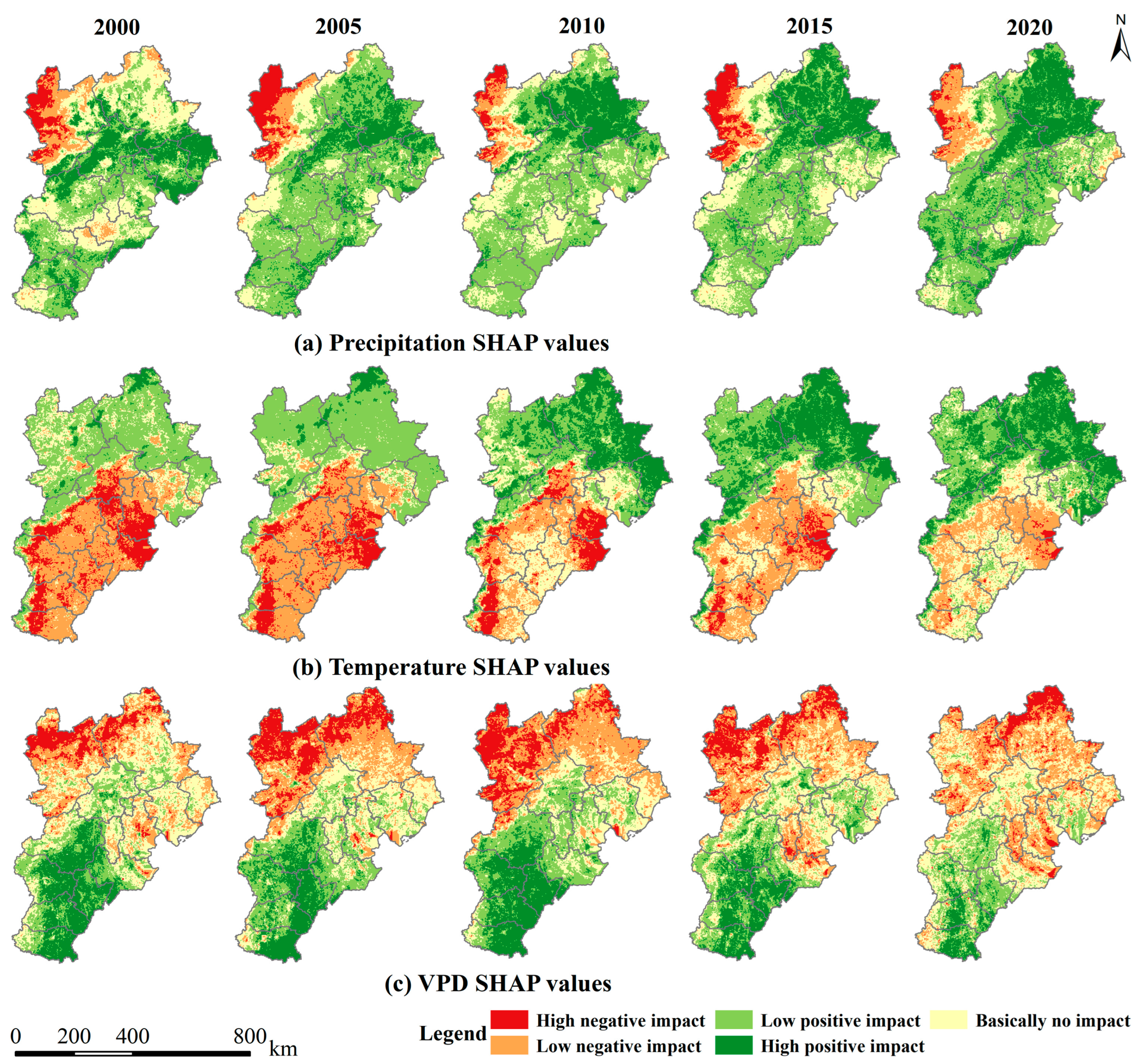
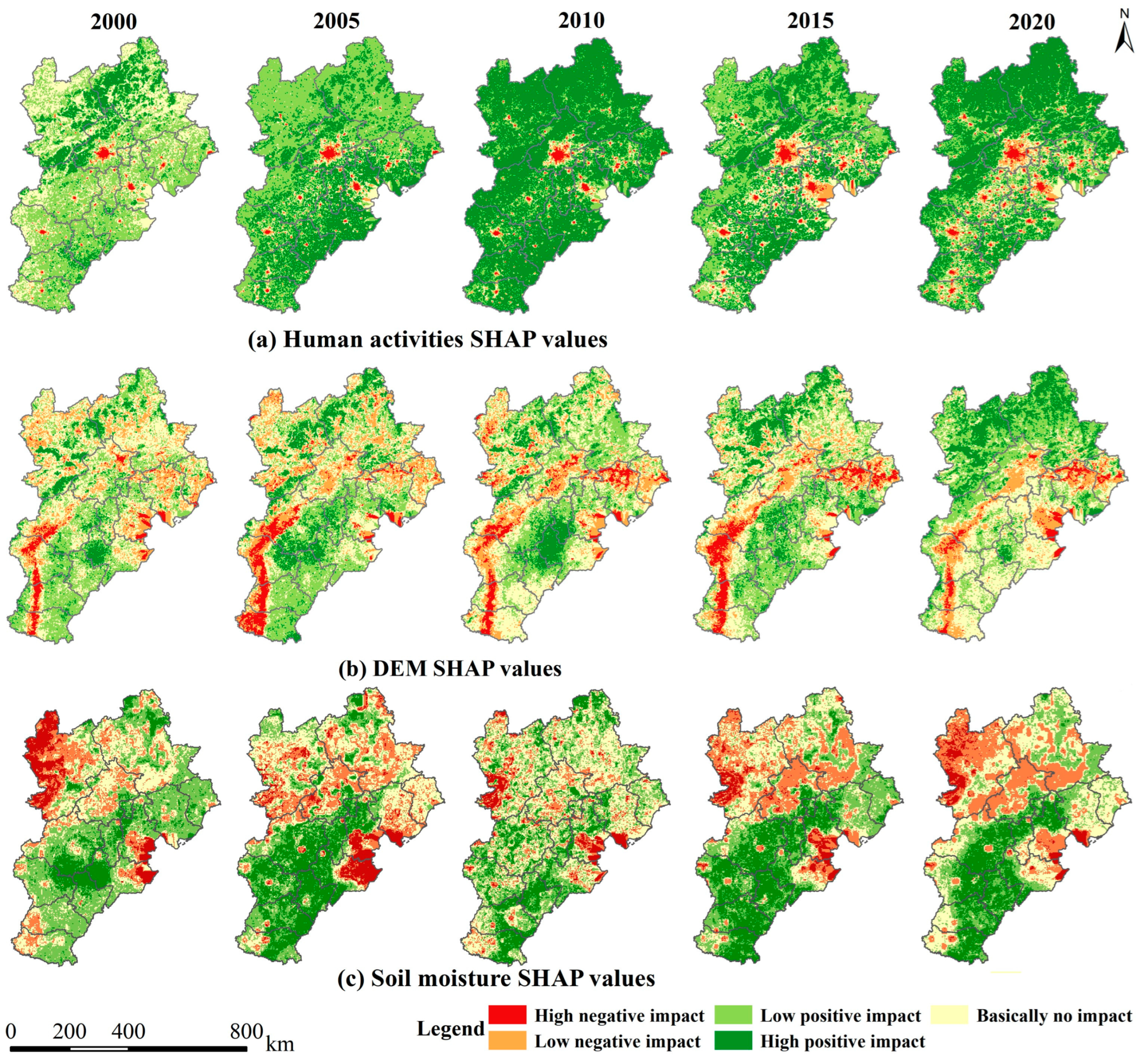
To quantify the magnitude and spatial pattern of the impact of each predictor on vegetation, the SHAP values of precipitation, temperature, VPD, HA, DEM, and SM were spatially interpolated. Based on this, the interpolation results for each factor were uniformly classified into five levels using the natural breaks method (Table 4): high negative impact, low negative impact, basically no impact, low positive impact, and high positive impact. This yielded the spatial distribution of SHAP values for each influencing factor, as shown in Figure 8 and Figure 9.
In Zhangjiakou, where meadows dominated with poor vegetation cover and limited annual precipitation, excessive rainfall led to soil erosion due to shallow grass roots, negatively affecting vegetation growth [58]. Consequently, the region showed significant negative precipitation impacts (Figure 8). By 2020, ecological restoration projects had improved vegetation conditions, reducing areas with strong negative precipitation effects. In contrast, the northwestern mountainous areas, characterized by abundant forests and grasslands, benefitted most from precipitation. The southern plains exhibited relatively high precipitation that met the substantial water demands of croplands, resulting in increasingly positive precipitation impacts on vegetation. These patterns demonstrated that precipitation’s effect on NDVI strongly correlated with local vegetation characteristics. In areas with lower NDVI, the negative impact of precipitation is more pronounced, whereas the positive impact is greater in areas where NDVI is higher. Temperature’s impact on NDVI showed increasingly positive effects in northwestern mountainous regions, while its negative effects gradually diminished in southeastern plains. The higher altitude northwestern areas benefited from suitable growing-season temperatures, which enhanced vegetation physiological activity and growth. In contrast, higher growing-season temperatures in the lower-altitude southern plains intensified moisture stress, thereby limiting growth. Temperature SHAP values exhibited significant variations along the Taihang Mountains, reflecting differences in topography and land use. VPD demonstrated an opposite influence pattern to temperature on NDVI, and the arid climate in the northwestern mountainous regions strongly hindered vegetation growth. However, with the implementation of ecological restoration projects, the impact of VPD on vegetation had gradually lessened.
During the past decade, urban expansion in the BTH region has intensified, with both the scope and intensity of HA continually increasing. This had led to widespread conversion of cropland and natural land into urban uses. The strongly negative impacts of HA were particularly pronounced and expanding in rapidly urbanizing cities such as Beijing, Tianjin, Shijiazhuang, and Tangshan (Figure 9). DEM negative impacts were mainly observed in transition zones between northwestern mountains and plains, as well as eastern coastal areas. The northwestern mountain plain border region, characterized by meadows and shrubs with poor vegetation cover, has seen improved vegetation conditions through implementation of the Taihang Mountains Afforestation Project and Three-North Shelterbelt Program, thereby reducing the adverse effect of DEM. However, proximity to plains with frequent urban expansion and agricultural activities limited potential for large scale forest growth in these transitional zones. SM showed considerable negative impacts on NDVI in northwestern Zhangjiakou and coastal areas, while exerting positive effects across southern plains. Zhangjiakou’s plateau climate supported mainly grasslands and planted vegetation, with naturally low SM and limited irrigation. The high negative impact observed in the southeastern coast may be partially attributed to the partial missing data on SM in some areas, which could lead to deviations in the results. In contrast, the southern plains benefit from extensive irrigation systems and high soil moisture levels that significantly promote corn and wheat growth.

3.5. Influencing Factor Change Analysis of the NDVI for Different Land Use Types

Significant changes occurred in land use classifications during the study period (Table 5). Urban expansion drove substantial conversion of cropland and grassland to urban and built-up areas, with cropland decreasing by approximately 9935.02 km2 and grassland declining by approximately 1384.85 km2, while urban areas expanded by approximately 10,244.81 km2. Concurrently, forestry initiatives like the Grain-for-Green Program and Three-North Shelterbelt Program had increased the forest area by approximately 765.61 km2.
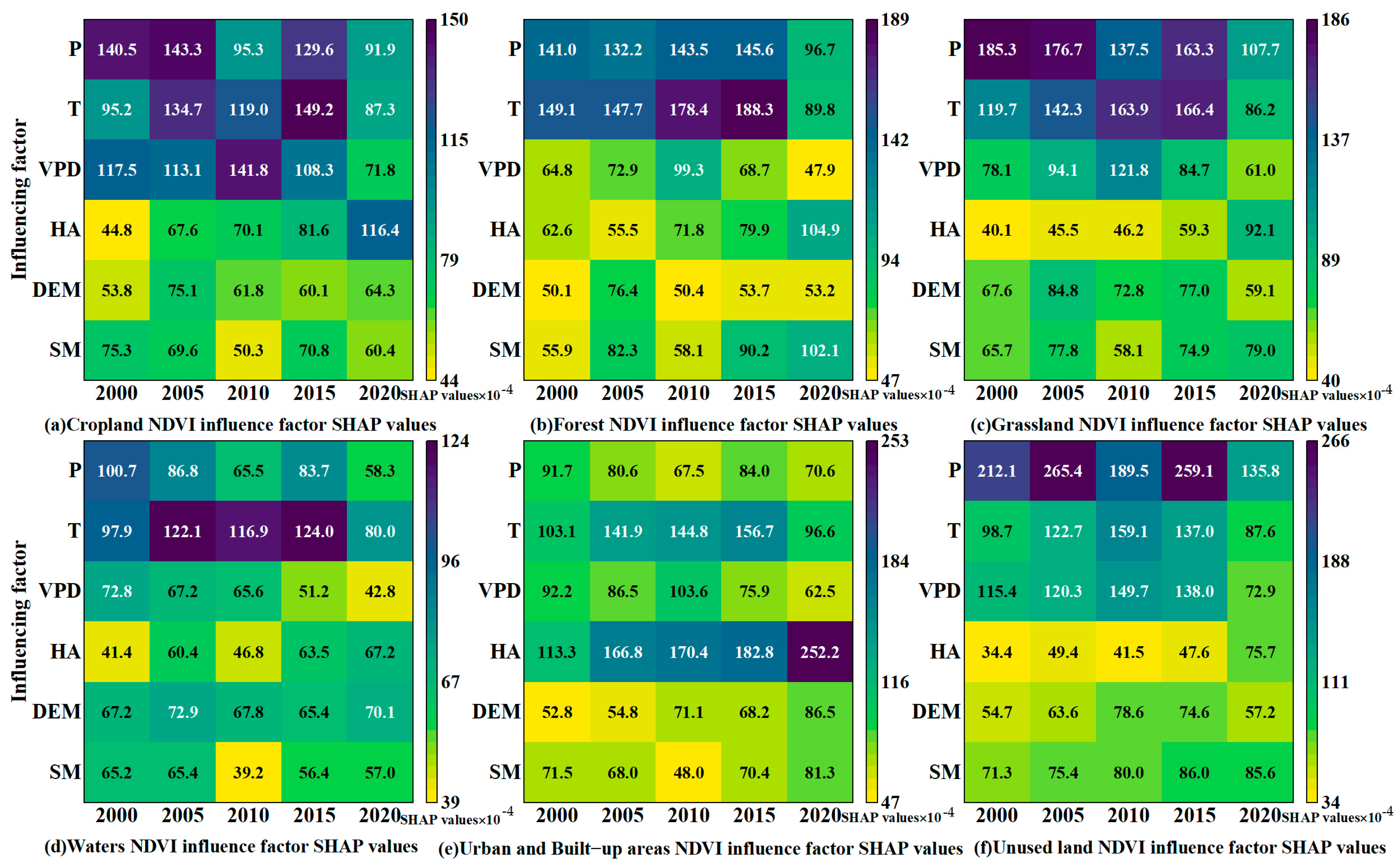
Based on the spatial distribution of SHAP values of influencing factors and the spatial distribution of land use in each period, the total SHAP values of influencing factors for each land use type were aggregated at the unit level, with the results shown in Figure 10. During the study period, land use changes correspondingly affected the variation in SHAP values. Over the years, the primary predictor for cropland NDVI was precipitation, followed by temperature. During the period of 2000–2005, the SHAP value for precipitation was higher than that for temperature, while from 2010 onward, the SHAP value for temperature gradually exceeded that of precipitation. By 2020, the SHAP values for both temperature and precipitation were lower than that of HA. For croplands dominated by summer corn and winter wheat cultivation, precipitation exerted greater influence during years with higher rainfall and lower temperatures, whereas temperature became more impactful in years with less precipitation and higher temperatures. However, intensified agricultural practices and urban expansion have aggravated the adverse effects of HA. The implementation of the Grain for Green Program during the study period facilitated the conversion of high elevation croplands to forests and grasslands, thereby reducing the impact of DEM on cropland NDVI. Furthermore, expanded precipitation patterns coupled with increased irrigation coverage progressively weakened the effect of SM on vegetation dynamics.
The primary long-term predictor influencing forest NDVI changes was temperature. During the period 2000–2015, temperature exhibited the highest SHAP value, exerting the most significant impact on forest NDVI, followed by precipitation. Forests in the BTH region are predominantly located in the climatically suitable northwestern mountains, consisting mainly of temperate coniferous and deciduous broadleaf species that respond strongly to temperature variations. Previous research confirms that when precipitation satisfies basic growth requirements, temperature becomes vegetation’s most sensitive climatic factor [59]. In grassland ecosystems, precipitation was the primary factor of NDVI, followed by temperature and VPD. Sparsely vegetated grasslands proved particularly vulnerable to moisture variability, though precipitation’s influence diminished as vegetation cover improved. Both forest and grassland systems, constituting the region’s primary natural vegetation in northwestern mountainous areas, demonstrated long-term positive responses to temperature and precipitation variations. In urban and built-up areas, NDVI was primarily influenced by human activity (HA), with its impact gradually increasing over time. Temperature had a stronger effect than precipitation on vegetation in these areas. Urban vegetation consisted largely of irrigated green spaces, whose sensitivity to temperature was amplified by the urban heat island effect. In water areas, vegetation coverage was generally sparse and declining, with temperature acting as the primary factor. In unused land areas, vegetation coverage was extremely poor and was strongly influenced by moisture conditions.

4. Discussion

4.1. Change Trend and Influencing Factors of NDVI

During the study period, the NDVI change in the BTH region exhibited significant spatial heterogeneity. Generally, vegetation improved in the northwest but declined in the southeast. This pattern aligned with findings from related studies [10,60]. The northwestern mountainous areas are largely covered by forests and grasslands and experience minimal human disturbance. There, ecological restoration projects such as afforestation have promoted sustained growth in vegetation NDVI. In contrast, the southeastern plains experienced strong HA. Urbanization in particular drove widespread vegetation degradation. The primary predictors of vegetation changes in the BTH region were precipitation, temperature, and HA. According to SHAP values, the relative importance of these predictors shifted over time. Precipitation was the primary influencing predictors in 2000 and 2005, temperature became the primary predictor in 2010 and 2015, and HA emerged as the primary predictor by 2020. This finding shared some similarities with studies based on linear models [57,58]. Both suggested that precipitation and temperature had significant impacts on vegetation changes. However, differences existed in the magnitude of these effects. These discrepancies likely arise from the limitations of linear methods in identifying complex nonlinear relationships. In contrast, Jiang et al. employed RF to investigate the impacts of climate and human activities on vegetation EVI in the BTH region [43]. They concluded that temperature and HA were the main factors influencing vegetation changes. This aligned with the nonlinear modeling philosophy and results of our study. A limitation of this study is the use of five-year averaged meteorological data, which could potentially mask the immediate impacts of extreme climate events, including droughts. However, the XGBoost-SHAP method employed in this study offered high-precision fitting and factor analysis capabilities. It not only revealed the temporal evolution patterns of predictor influences but also effectively characterized their spatial heterogeneity. This helped address the limitations of machine learning methods in quantitatively interpreting influencing factors from spatio-temporal perspectives.
Furthermore, this study integrated multi-dimensional indicators such as nighttime light and land use to more accurately assess the impacts of HA, with a particular focus on agricultural activities and urban expansion. The results showed that urban areas increased by over 50% from 2000 to 2020 (Table 5). Furthermore, the influence of HA on vegetation had continued to intensify (Figure 7), and its negative impacts have been expanding in urban peripheral areas (Figure 9a). Thus, agricultural activities and urban expansion were the primary human factors of NDVI trend changes, which aligned with previous research [60,61]. However, due to data limitations, this study employs five-year intervals and consequently lacks analysis of vegetation changes and their drivers at annual and seasonal scales. This may influence the results. Addressing these temporal scales represents an important direction for future research.

4.2. Uniqueness and Uncertainty of the XGBoost-SHAP Method

The XGBoost-SHAP method demonstrates strong data-fitting capabilities and provides clear, precise interpretations of NDVI changes and their influencing factors. Based on the simulation error metrics (Table 3), the XGBoost model achieved the lowest MAE and RMSE, outperforming RF, SVM, and KNN. Additionally, the XGBoost model was employed to simulate vegetation NDVI over five periods, achieving R2 values consistently greater than 0.96, along with small MAE and RMSE values. These results indicated that the model maintained strong consistency and stability across different temporal datasets. It also exhibited high predictive accuracy and generalization capability.
SHAP value analysis revealed that factor importance varies significantly across different spatio-temporal contexts. Although a single factor’s importance might decrease in comprehensive analysis, its geographic distribution pattern may remain unchanged. According to China’s climate zoning proposed [62], nearly the entire BTH region falls within semi-humid zones, with only a small northwestern portion classified as semi-arid. The distribution of precipitation SHAP value indicates that although precipitation’s overall importance has declined, its negative impact persists specifically in the semi-arid northwestern area of Zhangjiakou. This region is characterized by consistently low annual precipitation. Notably, the spatial extent of precipitation’s negative impact remained stable, but its intensity gradually weakened following the implementation of the Three-North Shelter Forest Program.
The primary limitation of the XGBoost-SHAP method lies in its assumption of feature independence. In real-world ecological environments, however, various factors generally exhibit complex interactions. Additionally, this study did not account for spatial autocorrelation in the data, which may affect the model’s generalizability and the accurate interpretation of feature importance. Furthermore, the use of random segmentation may lead to a lack of independence between the training and test sets, potentially overestimating the model’s performance. Nevertheless, comparative analysis with existing research findings and actual conditions indicated that the interpretation results of XGBoost-SHAP demonstrated strong credibility. To address the segmentation issue, subsequent research will explore using Spatial Block Cross-Validation to replace the random strategy. It should be noted that the XGBoost-SHAP method does not attempt to fully capture the behavior of the vegetation ecosystem, but rather provides an approximate explanation [63]. Consequently, the model’s reliability depends more critically on the appropriateness of selected features. In this study, we selected 14 features encompassing climate, terrain, hydrological conditions, and HA based on previous research. However, these features may introduce certain interference during model construction and interpretation, and some potentially influential factors might have been overlooked. Furthermore, lag in data selection may somewhat diminish the timeliness and application value of the research findings.

4.3. The Positive Influence of Human Activities

Forest cover increased substantially by 2020 compared to 2000 levels (Table 5), with progressive expansion observed not only in the northwestern hilly regions but also across eastern coastal areas and southern plains (Figure 3b). This vegetation recovery primarily resulted from major afforestation initiatives implemented throughout the BTH region, particularly the Three-North Shelterbelt Program initiated in 1978, the Taihang Mountain Greening Program established in 1986, and the Beijing-Tianjin Sandstorm Source Control Program launched in 2002. China’s Forestry and Grassland Statistical Yearbook recorded a total afforestation area of 89,277.96 km2 in the BTH region from 2000 to 2020, with these programs making substantial contributions to regional vegetation recovery [64,65]. Due to the complexity of human influence mechanisms and the lack of spatial afforestation data, this study could not precisely quantify the ecological impact of forestry projects or effectively distinguish the independent effects of different ecological programs, potentially affecting the accuracy of our findings [66]. Therefore, the selected human activity indicators may not fully reflect the actual intensity of policy implementation or the effectiveness of governance. In subsequent research, we will plan to employ the deviation between observed vegetation change rates and regional averages to better quantify human contributions to vegetation coverage changes. These derived metrics, combined with available afforestation records, will serve as key input variables for more sophisticated modeling using the XGBoost-SHAP framework.

4.4. Policy Implications

Based on the varying primary influencing factors of vegetation in different regions, targeted measures should be implemented. In the northwestern mountainous areas, vegetation was primarily driven by climate, necessitating enhanced differentiated conservation of forests and grasslands. In the southeastern plains, vegetation was primarily driven by human activities, requiring emphasis on water-saving practices for croplands and greening of urban and built-up areas, while curbing unregulated expansion. Additionally, positive regulation of human activities should be strengthened. In response to the increasing influence of human activities, ecological restoration in fragile areas should rely on engineering measures to improve water conditions, while urban and built-up areas should focus on enhanced greening planning to counterbalance the impacts of land expansion. This approach aims to redirect human activities toward ecological improvement.

5. Conclusions

The aim of this study is to quantitatively analyze the impacts of climate and human factors on vegetation change. We employed the XGBoost-SHAP method to identify and rank the most influential factors affecting vegetation growth. Additionally, we spatially decomposed the contribution of each factor to the NDVI trend. Finally, we investigated the primary factors influencing NDVI across different land-use types. The main conclusions are as follows:
(1)
From 2000 to 2020, vegetation cover in the BTH region increased overall. The primary factors of vegetation change were precipitation, temperature, and HA, with precipitation and temperature alternately dominating in different years. However, HA became the primary factor in 2020. Although anthropogenic impacts were less significant than climatic factors overall, their negative influence on NDVI gradually intensified over time.
(2)
Regional variations in the impacts of temperature, precipitation, and HA on NDVI were evident. Most vegetation greening occurred in forest and grassland areas within the northwestern hilly region, where temperature was the primary factor for forests, while precipitation primarily influenced grasslands. In contrast, vegetation browning was concentrated in the southeastern plains, particularly in urban and built-up areas and croplands. Here, precipitation dominated NDVI trends in croplands, whereas HA was the key driver in urban areas.
(3)
We employed the XGBoost-SHAP method for NDVI prediction, which achieved high accuracy (R2 > 0.96) and outperformed RF, SVM, and KNN. With robust data analysis capabilities, the method not only revealed the spatial heterogeneity of different influencing factors but also effectively tracked their temporal variations at different time points. It provided clearer insights into NDVI changes and their prediction factors. The study offered a novel methodological reference for in-depth understanding and analysis of the influence patterns of NDVI to climate change and HA.

Author Contributions

Conceptualization, Y.C. and H.W.; methodology, Y.C. and L.G.; software, L.G.; formal analysis, A.Z.; data curation, L.G.; writing—original draft preparation, Y.C. and L.G.; writing—review and editing, H.W. and A.Z.; visualization, Y.C. and L.G.; supervision, H.W. All authors have read and agreed to the published version of the manuscript.

Funding

This research was funded by National Natural Science Foundation of China [No. 42171212].

Data Availability Statement

The original data that support the findings of this study are contained within the article. Further inquiries can be directed to the corresponding author.

Acknowledgments

The authors are deeply thankful to the reviewers for their insightful comments and suggestions, which significantly contributed to the improvement of the manuscript.

Conflicts of Interest

The authors declare no conflicts of interest.

Appendix A

Figure A1. Trends of temperature and precipitation in the Beijing-Tianjin-Hebei region from 2000 to 2020: (a) average precipitation trend, (b) average temperature trend.
Forests 16 01873 g0a1

References

  1. Ouyang, Z.; Zheng, H.; Xiao, Y.; Polasky, S.; Liu, J.; Xu, W.; Wang, Q.; Zhang, L.; Xiao, Y.; Rao, E.; et al. Improvements in ecosystem services from investments in natural capital. Science 2016, 352, 1455–1459. [Google Scholar] [CrossRef] [PubMed]
  2. Mehmood, K.; Anees, S.A.; Rehman, A.; Pan, S.; Tariq, A.; Zubair, M.; Liu, Q.; Rabbi, F.; Khan, K.A.; Luo, M. Exploring spatiotemporal dynamics of ndvi and climate-driven responses in ecosystems: Insights for sustainable management and climate resilience. Ecol. Informatics 2024, 80, 102532. [Google Scholar] [CrossRef]
  3. Gong, Z.; Ge, W.; Guo, J.; Liu, J. Satellite remote sensing of vegetation phenology: Progress, challenges, and opportunities. ISPRS J. Photogramm. Remote Sens. 2024, 217, 149–164. [Google Scholar] [CrossRef]
  4. Piao, S.; Wang, X.; Lian, X.; He, Y.; Ciais, P.; Park, T.; Chen, C.; Myneni, R.B.; Nemani, R.R.; Bjerke, J.W. Characteristics, drivers and feedbacks of global greening. Nat. Rev. Earth Environ. 2020, 1, 14–27. [Google Scholar] [CrossRef]
  5. Bao, Z.; Zhang, J.; Wang, G.; Guan, T.; Jin, J.; Liu, Y.; Li, M.; Ma, T. The sensitivity of vegetation cover to climate change in multiple climatic zones using machine learning algorithms. Ecol. Indic. 2021, 124, 107443. [Google Scholar] [CrossRef]
  6. He, J.; Shi, X.; Fu, Y. Identifying vegetation restoration effectiveness and driving factors on different micro-topographic types of hilly loess plateau: From the perspective of ecological resilience. J. Environ. Manag. 2021, 289, 112562. [Google Scholar] [CrossRef]
  7. Li, Z.; Sun, R.; Zhang, J.; Zhang, C. Temporal-spatial analysis of vegetation coverage dynamics in Beijing-Tianjin-Hebei metropolitan regions. Acta Ecol. Sin. 2017, 37, 7418–7426. [Google Scholar] [CrossRef]
  8. Gao, S.; Dong, G.; Jiang, X.; Nie, T.; Guo, X. Analysis of factors influencing spatiotemporal differentiation of the NDVI in the upper and middle reaches of the Yellow River from 2000 to 2020. Front. Environ. Sci. 2023, 10, 1072430. [Google Scholar] [CrossRef]
  9. Darabi, H.; Haghighi, A.T.; Klve, B.; Luoto, M. Remote sensing of vegetation trends: A review of methodological choices and sources of uncertainty. Remote Sens. Appl. Soc. Environ. 2025, 37, 101500. [Google Scholar] [CrossRef]
  10. Zhao, Y.; Sun, R.; Ni, Z. Identification of Natural and Anthropogenic Drivers of Vegetation Change in the Beijing-Tianjin-Hebei Megacity Region. Remote Sens. 2019, 11, 1224. [Google Scholar] [CrossRef]
  11. Kelsey, K.C.; Pedersen, S.H.; Leffler, A.J.; Sexton, J.O.; Feng, M.; Welker, J.M. Winter snow and spring temperature have differential effects on vegetation phenology and productivity across arctic plant communities. Glob. Change Biol. 2021, 27, 1572–1586. [Google Scholar] [CrossRef] [PubMed]
  12. Xiang, J.; Peng, W.; Tao, S. Spatio-temporal Changes of Vegetation NDVI and Its Topographic Response in the Upper Reaches of the Minjiang River from 2000 to 2020. Resour. Environ. Yangtze Basin 2022, 31, 1534–1547. [Google Scholar]
  13. Liu, Z.; Chen, Y.; Chen, C. Analysis of the Spatiotemporal Characteristics and Influencing Factors of the NDVI Based on the GEE Cloud Platform and Landsat Images. Remote Sens. 2023, 15, 4980. [Google Scholar] [CrossRef]
  14. Du, R.; Wu, J.; Tian, F.; Yang, J.; Han, X.; Chen, M.; Zhao, B.; Lin, J. Reversal of soil moisture constraint on vegetation growth in North China. Sci. Total Environ. 2023, 865, 161246. [Google Scholar] [CrossRef]
  15. Liu, T.; Zhang, Q.; Li, T.; Zhang, K. Dynamic Vegetation Responses to Climate and Land Use Changes over the Inner Mongolia Reach of the Yellow River Basin, China. Remote Sens. 2023, 15, 3531. [Google Scholar] [CrossRef]
  16. Ran, Q.; Hao, Y.; Xia, A.; Liu, W.; Hu, R.; Cui, X.; Xue, K.; Song, X.; Xu, C.; Ding, B.; et al. Quantitative Assessment of the Impact of Physical and Anthropogenic Factors on Vegetation Spatial-Temporal Variation in Northern Tibet. Remote Sens. 2019, 11, 1183. [Google Scholar] [CrossRef]
  17. Fan, X.; Gao, P.; Tian, B.; Wu, C.; Mu, X. Spatio-Temporal Patterns of NDVI and Its Influencing Factors Based on the ESTARFM in the Loess Plateau of China. Remote Sens. 2023, 15, 2553. [Google Scholar] [CrossRef]
  18. Chang, S.; Wang, J.; Zhang, F.; Niu, L.; Wang, Y. A study of the impacts of urban expansion on vegetation primary productivity levels in the Jing-Jin-Ji region, based on nighttime light data. J. Clean. Prod. 2020, 263, 121490. [Google Scholar] [CrossRef]
  19. Zhao, Y.; Hu, C.; Dong, X.; Li, J. NDVI Characteristics and Influencing Factors of Typical Ecosystems in the Semi-Arid Region of Northern China: A Case Study of the Hulunbuir Grassland. Land 2023, 12, 713. [Google Scholar] [CrossRef]
  20. Wang, H.; Yan, S.; Ciais, P.; Wigneron, J.P.; Liu, L.; Li, Y.; Fu, Z.; Ma, H.; Liang, Z.; Wei, F.; et al. Exploring complex water stress–gross primary production relationships: Impact of climatic drivers, main effects, and interactive effects. Glob. Change Biol. 2022, 28, 4110–4123. [Google Scholar] [CrossRef]
  21. Liu, H.; Liu, Y.; Chen, Y.; Fan, M.; Chen, Y.; Gang, C.; You, Y.; Wang, Z. Dynamics of global dryland vegetation were more sensitive to soil moisture: Evidence from multiple vegetation indices. Agric. For. Meteorol. 2023, 331, 109327. [Google Scholar] [CrossRef]
  22. Tuoku, L.; Wu, Z.; Men, B. Impacts of climate factors and human activities on ndvi change in china. Ecol. Inform. 2024, 81, 102555. [Google Scholar] [CrossRef]
  23. Xu, Y.; Huang, W.; Jing, J.; Zhang, Z.; Li, M.; Ou, Y.; Lu, M.; Dou, S. Dynamic Variation of Vegetation Cover and Its Relation with Climate Variables in Beijing-Tianjin-Hebei Region. Bull. Soil Water Conserv. 2020, 40, 319–327. [Google Scholar] [CrossRef]
  24. Liu, W.; Jiao, S.; An, Q.; Li, Y.; Zhang, J.; Mo, Y.; Shao, Y.; Feng, Y. Impacts of Climate Change and Human Activities on NDVI in Guizhou Province from 1998 to 2018. Resour. Environ. Yangtze Basin 2021, 30, 2883–2895. [Google Scholar]
  25. Zhang, Y.; Jiang, X.; Lei, Y.; Gao, S. The contributions of natural and anthropogenic factors to NDVI variations on the Loess Plateau in China during 2000–2020. Ecol. Indic. 2022, 143, 109342. [Google Scholar] [CrossRef]
  26. Zhang, D.; Jia, Q.; Wang, P.; Zhang, J.; Hou, X.; Li, X.; Li, W. Analysis of spatial variability in factors contributing to vegetation restoration in Yan’an, China. Ecol. Indic. 2020, 113, 106278. [Google Scholar] [CrossRef]
  27. Wang, Y.; Hao, L.; Xu, Q.; Li, J.; Chang, H. Spatio-temporal variations of vegetation coverage and its geographical factors analysis on the Loess Plateau from 2001 to 2019. Acta Ecol. Sin. 2023, 43, 2397–2407. [Google Scholar] [CrossRef]
  28. Wang, J.; Li, X.; Christakos, G.; Liao, Y.; Zhang, T.; Gu, X.; Zheng, X. Geographical detectors-based health risk assessment and its application in the neural tube defects study of the Heshun Region, China. Int. J. Geogr. Inf. Sci. 2010, 24, 107–127. [Google Scholar] [CrossRef]
  29. Xia, J.; Ma, M.; Liang, T.; Wu, C.; Yang, Y.; Zhang, L.; Zhang, Y.; Yuan, W. Estimates of grassland biomass and turnover time on the Tibetan Plateau. Environ. Res. Lett. 2018, 13, 014020. [Google Scholar] [CrossRef]
  30. Li, X.; Yuan, W.; Dong, W. A Machine Learning Method for Predicting Vegetation Indices in China. Remote Sens. 2021, 13, 1147. [Google Scholar] [CrossRef]
  31. Shi, Y.; Jin, N.; Ma, X.; Wu, B.; He, Q.; Yue, C.; Yu, Q. Attribution of climate and human activities to vegetation change in China using machine learning techniques. Agric. For. Meteorol. 2020, 294, 108146. [Google Scholar] [CrossRef]
  32. Anees, S.A.; Mehmood, K.; Rehman, A.; Rehman, N.U.; Muhammad, S.; Shahzad, F.; Hussain, K.; Luo, M.; Alarfaj, A.A.; Alharbi, A.A.; et al. Unveiling fractional vegetation cover dynamics: A spatiotemporal analysis using MODIS NDVI and machine learning. Environ. Sustain. Indic. 2024, 24, 100485. [Google Scholar] [CrossRef]
  33. Ma, N.; Cao, S.; Bai, T.; Yang, Z.; Cai, Z.; Sun, W. Assessment of Vegetation Dynamics in Xinjiang Using NDVI Data and Machine Learning Models from 2000 to 2023. Sustainability 2025, 17, 306. [Google Scholar] [CrossRef]
  34. Lundberg, S.M.; Erion, G.; Chen, H.; DeGrave, A.; Prutkin, J.M.; Nair, B.; Katz, R.; Himmelfarb, J.; Bansal, N.; Lee, S.I. From local explanations to global understanding with explainable AI for trees. Nat. Mach. Intell. 2020, 2, 56–67. [Google Scholar] [CrossRef]
  35. Lundberg, S.M.; Lee, S.I. A Unified Approach to Interpreting Model Predictions. Adv. Neural Inf. Process. Syst. 2017, 30, 4768–4777. [Google Scholar]
  36. Li, L.; Zeng, Z.; Zhang, G.; Duan, K.; Liu, B.; Cai, X. Exploring the Individualized Effect of Climatic Drivers on MODIS Net Primary Productivity through an Explainable Machine Learning Framework. Remote Sens. 2022, 14, 4401. [Google Scholar] [CrossRef]
  37. Li, K.; Zhao, J.; Li, Y.; Lin, Y. Identifying trade-offs and synergies among land use functions using an XGBoost-SHAP model: A case study of Kunming, China. Ecol. Indic. 2025, 172, 113330. [Google Scholar] [CrossRef]
  38. Yao, X.; Fang, S. Exploring the coupling of ecosystem services and human well-being: Evidence from Chinese cities through interpretable machine learning. Ecol. Indic. 2025, 180, 114315. [Google Scholar] [CrossRef]
  39. Lu, J.; Liu, X.; Zhu, D.; Zhang, S. Unveiling multiscale and nonlinear effects of land use change drivers through interpretable machine learning model: Insights from “Ecological-cost and Economic-benefit” trade-off perspective. Environ. Impact Assess. Rev. 2026, 118, 108254. [Google Scholar] [CrossRef]
  40. Dikshit, A.; Pradhan, B. Interpretable and explainable AI (XAI) model for spatial drought prediction. Sci. Total Environ. 2021, 801, 149797. [Google Scholar] [CrossRef]
  41. Lai, Y.; Wan, G.; Qin, X. Decoding China’s new-type industrialization: Insights from an XGBoost-SHAP analysis. J. Clean. Prod. 2024, 478, 143927. [Google Scholar] [CrossRef]
  42. Yan, S.; Wang, H.; Jiao, K. Spatiotemporal Dynamics of NDVI in the Beijing-Tianjin-Hebei Region based on MODIS Data and Quantitative Attribution. J. Geo-Inf. Sci. 2019, 21, 767–780. [Google Scholar] [CrossRef]
  43. Jiang, M.; He, Y.; Song, C.; Pan, Y.; Qiu, T.; Tian, S. Disaggregating climatic and anthropogenic influences on vegetation changes in Beijing-Tianjin-Hebei region of China. Sci. Total Environ. 2021, 786, 147574. [Google Scholar] [CrossRef]
  44. Yao, Y. Pattern and change of NDVI and their environmental influencing factors for 1986–2019 in the Qinling-Daba Mountains of central China. Front. For. Glob. Change 2024, 7, 1372488. [Google Scholar] [CrossRef]
  45. Peng, S.; Ding, Y.; Liu, W.; Li, Z. 1km monthly temperature and precipitation dataset for China from 1901 to 2017. Earth Syst. Sci. Data. 2019, 11, 1931–1946. [Google Scholar] [CrossRef]
  46. McNally, A. FLDAS Noah Land Surface Model L4 Global Monthly 0.1 × 0.1 Degree (MERRA-2 and CHIRPS). Goddard Earth Sciences Data and Information Services Center (GES DISC), v1. 2018. Available online: https://data.nasa.gov/dataset/fldas-noah-land-surface-model-l4-global-monthly-0-1-x-0-1-degree-merra-2-and-chirps-v001-f-af46e (accessed on 9 May 2024).
  47. Howell, T.A.; Dusek, D.A. Comparison of vapor-pressure-deficit calculation methods—Southern high plains. J. Irrig. Drain. Eng. 1995, 121, 191–198. [Google Scholar] [CrossRef]
  48. Zhang, T.; Zhang, Y.; Xu, M.; Zhu, J.; Chen, N.; Jiang, Y.; Huang, K.; Zu, J.; Liu, Y.; Yu, G. Water availability is more important than temperature in driving the carbon fluxes of an alpine meadow on the Tibetan Plateau. Agric. For. Meteorol. 2018, 256–257, 22–31. [Google Scholar] [CrossRef]
  49. Chen, Z.; Yu, B.; Yang, C.; Zhou, Y.; Yao, S.; Qian, X.; Wang, C.; Wu, B.; Wu, J. An extended time series (2000–2018) of global NPP-VIIRS-like nighttime light data from a cross-sensor calibration. Earth Syst. Sci. Data 2021, 13, 889–906. [Google Scholar] [CrossRef]
  50. Feng, X.; Tian, J.; Wang, Y.; Wu, J.; Liu, J.; Ya, Q.; Li, Z. Spatio-Temporal Variation and Climatic Driving Factors of Vegetation Coverage in the Yellow River Basin from 2001 to 2020 Based on kNDVI. Forests 2023, 14, 620. [Google Scholar] [CrossRef]
  51. Waked, A.; Sauvage, S.; Borbon, A.; Gauduin, J.; Pallares, C.; Vagnot, M.P.; Léonardis, T.; Locoge, N. Multi-year levels and trends of non-methane hydrocarbon concentrations observed in ambient air in France. Atmos. Environ. 2016, 141, 263–275. [Google Scholar] [CrossRef]
  52. Chen, T.; Guestrin, C. Xgboost: A scalable tree boosting system. In Proceedings of the 22nd Acm Sigkdd International Conference on Knowledge Discovery and Data Mining, San Francisco, CA, USA, 13–17 August 2016; pp. 785–794. [Google Scholar] [CrossRef]
  53. Mousa, S.R.; Bakhit, P.R.; Ishak, S. An extreme gradient boosting method for identifying the factors contributing to crash/near-crash events: A naturalistic driving study. Can. J. Civ. Eng. 2019, 46, 712–721. [Google Scholar] [CrossRef]
  54. Štrumbelj, E.; Kononenko, I. Explaining prediction models and individual predictions with feature contributions. Knowl. Inf. Syst. 2014, 41, 647–665. [Google Scholar] [CrossRef]
  55. Ribeiro, M.T.; Singh, S.; Guestrin, C. “Why should I trust you?” Explaining the predictions of any classifier. In Proceedings of the 22nd ACM SIGKDD International Conference on Knowledge Discovery and Data Mining, San Francisco, CA, USA, 13–17 August 2016; pp. 1135–1144. [Google Scholar]
  56. Shapley, L.S. A value for n-person games. Contributions to the Theory of Games II (1953) 307-317. In Classics in Game Theory; Princeton University Press: Princeton, NY, USA, 1997; pp. 69–79. [Google Scholar]
  57. Yan, M.; Li, Z.; Tian, X.; Chen, E.; Gu, C. Remote sensing estimation of gross primary productivity and its response to climate change in the upstream of Heihe River Basin. Chin. J. Plant Ecol. 2016, 40, 1–12. [Google Scholar] [CrossRef]
  58. Qi, X.; Jia, J.; Liu, H.; Lin, Z. Relative importance of climate change and human activities for vegetation changes on China’s silk road economic belt over multiple timescales. Catena 2019, 180, 224–237. [Google Scholar] [CrossRef]
  59. Jiao, K.; Gao, J.; Wu, S.; Hou, W. Research progress on the response processes of vegetation activity to climate change. Acta Ecol. Sin. 2018, 38, 2229–2238. [Google Scholar] [CrossRef]
  60. Zhou, Q.; Zhao, X.; Wu, D.; Tang, R.; Du, X.; Wang, H.; Zhao, J.; Xu, P.; Peng, Y. Impact of Urbanization and Climate on Vegetation Coverage in the Beijing–Tianjin–Hebei Region of China. Remote Sens. 2019, 11, 2452. [Google Scholar] [CrossRef]
  61. Chang, Y.; Zhang, G.; Zhang, T.; Xie, Z.; Wang, J. Vegetation Dynamics and Their Response to the Urbanization of the Beijing–Tianjin–Hebei Region, China. Sustainability 2020, 12, 8550. [Google Scholar] [CrossRef]
  62. Zheng, J.; Yin, Y.; Li, B. A New Scheme for Climate Regionalization in China. Acta Geogr. Sin. 2010, 65, 3–12. [Google Scholar] [CrossRef]
  63. Mittelstadt, B.; Russell, C.; Wachter, S. Explaining Explanations in AI. In Proceedings of the Conference on Fairness, Accountability, and Transparency, FAT* ’19, Atlanta, GA, USA, 29–31 January 2019; Association for Computing Machinery: New York, NY, USA, 2019; pp. 279–288. [Google Scholar] [CrossRef]
  64. Cai, Y.; Zhang, F.; Duan, P.; Yung Jim, C.; Weng Chan, N.; Shi, J.; Liu, C.; Wang, J.; Bahtebay, J.; Ma, X. Vegetation cover changes in China induced by ecological restoration-protection projects and land-use changes from 2000 to 2020. Catena 2022, 217, 106530. [Google Scholar] [CrossRef]
  65. Yang, X.; Xu, B.; Jin, Y.; Qin, Z.; Ma, H.; Li, J.; Zhao, F.; Chen, S.; Zhu, X. Remote sensing monitoring of grassland vegetation growth in the Beijing–Tianjin sandstorm source project area from 2000 to 2010. Ecol. Indic. 2015, 51, 244–251. [Google Scholar] [CrossRef]
  66. Chen, Y.; Zhang, T.; Zhu, X.; Yi, G.; Li, J.; Bie, X.; Hu, J. Quantitatively analyzing the driving factors of vegetation change in China: Climate change and human activities. Ecol. Inform. 2024, 82, 102667. [Google Scholar] [CrossRef]
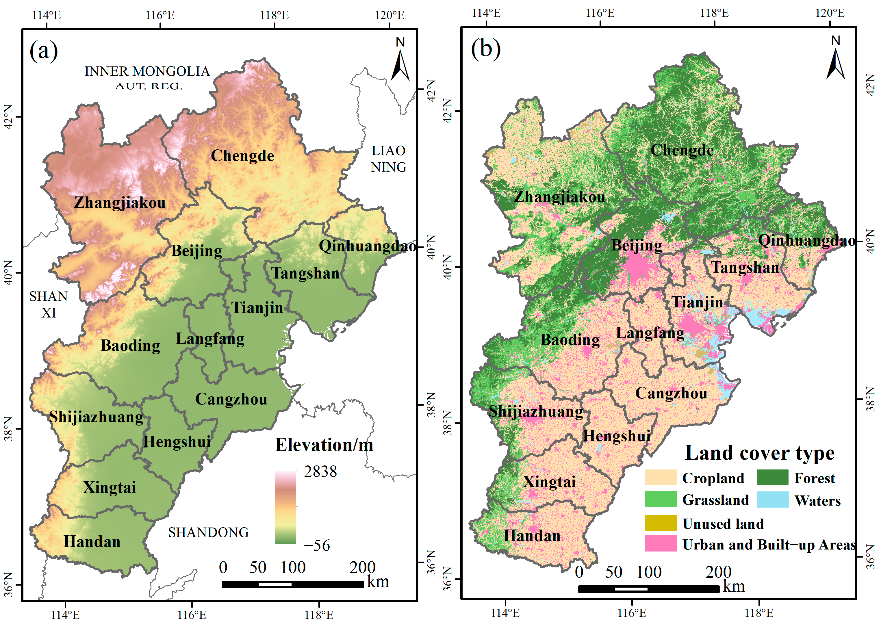
Figure 1. (a) Elevation and location of the BTH region. (b) Land use types in the BTH region in 2020 (Data source: Resource and Environment Science and Data Center of Chinese Academy of Sciences).
Forests 16 01873 g001
Figure 2. The workflow of the study.
Forests 16 01873 g002
Figure 3. The Spatial distribution of mean NDVI and trend of vegetation changes from 2000 to 2020.
Forests 16 01873 g003
Figure 4. Annual changes in the NDVI mean values of different land use types in the BTH region.
Forests 16 01873 g004
Figure 5. Probability density graph of predicted and original NDVI data over five phases.
Forests 16 01873 g005
Figure 6. SHAP value distribution plot for factors importance ranking.
Forests 16 01873 g006
Figure 7. Changes in the SHAP values for the main influencing factors in 2000–2020.
Forests 16 01873 g007
Figure 8. Spatial distribution of the SHAP values of precipitation, temperature, and VPD.
Forests 16 01873 g008
Figure 9. Spatial distribution of the SHAP values of human activities, DEM, and soil moisture.
Forests 16 01873 g009
Figure 10. Factors influencing the SHAP values of the different land use types.
Forests 16 01873 g010
Table 1. The influencing factors and data sources.
FactorSpatial
Resolution
Temporal ResolutionData Source
Vegetation conditions (NDVI)250 m 16 daysMODIS MOD13Q1
Climate conditions
Precipitation(P)1000 mmonthlyNational Earth System Science Data Center
Temperature(T)
Terrain (DEM)90 m-United States Geological Survey
Hydrological and soil conditions
Vapor pressure deficit (VPD)0.1°monthlyCalculated from the formula
Soil moisture
content (SM)
0–10 cmFLDAS (Noah Land Surface Model L4)
10–40 cm
40–100 cm
100–200 cm
Clay area proportion (Clay)1000 m-Resource and Environment Science and Data Center of Chinese Academy of Sciences
Changes in land use
Cropland proportion (CROP)1000 m5 yearsResource and Environment Science and Data Center of Chinese Academy of Sciences
Natural Vegetation area proportion (NV)
Impervious surface area proportion (IS)
Status of human activities
Population density (POP) 1000 m5 yearsResource and Environment Science and Data Center of Chinese Academy of Sciences
Nighttime light (NTL)1000 myearlyAn extended time-series (2000–2018) of global NPP-VIIRS-like nighttime light data
Variable description: The units for Precipitation, Temperature, Vapor pressure deficit, and Soil moisture content are mm, °C, kPa, and m3/m3, respectively. Clay area proportion and land use proportions (CROP, NV, IS) are expressed in percentage form.
Table 2. The percentages of areas with different vegetation change trends (unit: %).
Study Area and Land Use TypeVegetation Change Trends
Extremely Significant ReductionSignificant ReductionNon-Significant ReductionNon-Significant IncreaseSignificant IncreaseExtremely Significant Increase
BTH region4.85 3.50 16.86 26.83 11.59 36.37
cropland4.35 3.92 21.60 34.54 12.43 23.07
Forest0.82 0.85 5.18 15.47 12.06 65.48
Grassland1.03 1.03 6.33 19.40 12.61 59.22
Water area5.33 3.98 17.70 23.74 7.29 14.25
Urban and built-up areas17.87 8.83 29.06 23.98 5.93 11.17
Unused land3.09 2.85 17.50 31.46 14.80 25.91
Table 3. The evaluation index verification results.
YearModel(R2)(MAE)(RMSE)
2000KNN0.5170.5090.695
SVR0.6360.0770.083
RF0.7520.170.06
XGBoost0.9610.0190.026
2005XGBoost0.9690.0180.026
20100.9800.0140.019
20150.9820.0140.012
20200.9640.0180.025
Table 4. The level intervals of SHAP values for predictors.
ItemHigh Negative ImpactLow Negative ImpactBasically No ImpactLow Positive ImpactHigh Positive Impact
Precipitation<−0.092[−0.092, −0.041)[−0.041, −0.005)[−0.005, 0.015)≥0.015
Temperature<−0.039[−0.039, −0.018)[−0.018, 0.006)[0.006, 0.029)≥0.029
VPD<−0.023[−0.023, −0.008)[−0.008, 0.007)[0.007, 0.025)≥0.025
HA<−0.078[−0.078, −0.035)[−0.035, −0.007)[−0.007, 0.010)≥0.010
DEM<−0.029[−0.029, −0.014)[−0.014, −0.004)[−0.004, 0.007)≥0.007
SM<−0.031[−0.031, −0.015)[−0.015, −0.002)[−0.002, 0.012)≥0.012
Table 5. Area changes of different land use types in 2000–2020 (Unit: 103 km2).
YearLand Use Type
CroplandForest GrasslandWater AreaUrban and Built-Up Unused Land
2000109.82 44.72 35.42 6.47 17.86 2.08
2005108.42 44.85 35.20 6.30 19.57 2.02
2010104.01 44.96 34.04 5.73 26.17 1.49
2015102.51 44.83 33.82 5.68 28.16 1.41
202099.89 45.48 34.04 7.15 28.11 1.75
Change amount−9.94 0.77 −1.38 0.68 10.24 −0.33
Disclaimer/Publisher’s Note: The statements, opinions and data contained in all publications are solely those of the individual author(s) and contributor(s) and not of MDPI and/or the editor(s). MDPI and/or the editor(s) disclaim responsibility for any injury to people or property resulting from any ideas, methods, instructions or products referred to in the content.