Article

Individual-Tree Crown Width Prediction for Natural Mixed Forests in Northern China Using Deep Neural Network and Height Threshold Method

College of Forestry, Shanxi Agricultural University, Jinzhong 030810, China
*
Author to whom correspondence should be addressed.
Forests 2025, 16(12), 1778; https://doi.org/10.3390/f16121778
Submission received: 29 October 2025 / Revised: 18 November 2025 / Accepted: 24 November 2025 / Published: 26 November 2025

Abstract

Crown width (CW) is a critical metric for characterizing tree-canopy dimensions; however, its direct measurement remains labor-intensive and is often impractical in inaccessible crowns. Consequently, CW is frequently derived from projections, which are susceptible to multiple sources of imprecision, including canopy density, crown irregularity, terrain heterogeneity, and the observer’s vantage point, especially in structurally complex natural forests. While deep neural network (DNN) models show substantial potential for CW prediction, their performance in heterogeneous forests remains uncertain. We developed DNN models integrated with a Height Threshold Method (HTM) to predict individual-tree CW in the natural mixed forests of Northern China, dominated by Larix principis-rupprechtii and Picea asperata. Our study further compared the relative importance of feature engineering versus model architectural complexity in predictive accuracy and identified the key ecological variables governing CW. The model performance was evaluated through the coefficient of determination (R2), mean square error (MSE), mean absolute error (MAE), and mean absolute percentage error (MAPE). Field surveys of 34 representative sample plots produced 1884 individual-tree records. The main results were as follows: (1) all DNNs avoided overfitting, and were statistical stable under ten-fold cross-validation; (2) the optimized DNN3-2 model (tuned hidden layer count, neurons/hidden layer, L2 regularization, and dropout) achieved peak performance, explaining 69% of CW variance with residuals with stable variance and excellent coverage properties; (3) tree size, neighborhood competition, species identity, and site quality were the most important predictors; and (4) stand parameters calculated from competitive neighborhoods defined by the HTM, particularly mean stand crowding, Simpson’s index (1-D), and Shannon’s index (H′), significantly improved prediction accuracy. By integrating DNN with the HTM, our approach allows for accurate prediction of individual-tree CW in natural mixed forests of Northern China, dominated by Larix principis-rupprechtii and Picea asperata.

1. Introduction

The tree canopy is a pivotal interface between the tree and its environment, with its morphological characteristics directly governing key physiological processes such as photosynthesis, transpiration, and carbon allocation [1,2]. Consequently, crown dimensions (e.g., size and shape) serve as robust proxies for a tree’s physiological vitality and competitive ability [3,4,5], ultimately influencing critical outcomes including individual tree growth, productivity allocation [6,7], and wood quality [8,9,10]. Understanding these relationships allows for a series of inferences regarding forest ecosystem behavior—such as carbon sequestration dynamics, water cycling, and light competition—and is fundamental for simulating and predicting forest evolution under changing environmental conditions. This established link ultimately provides a critical support foundation for multi-criteria analysis and evidence-based decision-making by forest managers [11,12]. However, measuring canopy characteristics such as CW is not only more labor-intensive but also inherently less accurate than measuring stem metrics like diameter at breast height (DBH) [13,14] due to the practical inaccessibility of crowns and the methodological limitations of projection techniques, which are prone to errors from occlusion, terrain, and perspective. This practical limitation underscores the necessity for reliable canopy models to predict these ecologically significant traits from readily measured variables [15,16]. In response to the growing demand for intensive forest management, research on canopy modeling has gradually increased in recent years [17,18,19,20,21,22,23,24].
CW is a commonly used indicator of crown size, and numerous modeling approaches have been explored, including linear regression models [25], nonlinear regression models [20,25,26], linear mixed-effects models (LME) [13,27,28,29], nonlinear seemingly unrelated regression (NSUR) [14,22,30], generalized additive model (GAM) [22], nonlinear mixed effects models (NLME) [4,15,17,23,31,32,33], and generalized nonlinear mixed effects models (GNLME) [34,35]. Common predictors include tree size, competition, site quality, stand structure, and climate [15,16,24,34].
Machine learning techniques can capture complex and nonlinear interaction between predictive variables and response variables without relying on strict statistical assumptions or predetermined mathematical functional forms [36,37]. Numerous studies have shown that such techniques mostly perform better in predicting single tree growth compared to traditional regression methods [37,38,39]. As a more advanced form of machine learning, deep learning algorithms (DLA) have become prominent in many fields as an application of artificial intelligence techniques since 2010 [40,41,42,43]. DLA are also being rapidly deployed across diverse domains of forest ecology, including DBH-height allometric modeling [44,45], tree aboveground biomass prediction [46], and remote sensing-based forest inventory and planning [47,48,49]. For example, there were scholars introduced DLA into the single tree height diameter model of Pinus nigra aged pure forest in Anatolia, and found that the optimal deep learning model structure has better predictive ability than other structural deep learning models, artificial neural networks, nonlinear regression, and nonlinear mixed effects models [44]. There were other scholars as well constructed a simple deep neural network model to predict CW in natural spruce–fir–broadleaf mixed forests [16]. Their results indicated that under identical predictor combinations, the NLME model outperformed the DNN model; conversely, when all predictors were used, the opposite outcome was observed.
However, considerable uncertainties remain in developing DNN models for CW prediction in structurally complex natural forests, particularly regarding predictor selection and model architecture complexity design. Accordingly, this study addresses three questions: (1) How can predictor variables be optimized for CW modeling in structurally complex natural forests? (2) Does increasing model complexity necessarily improve DNN performance for individual-tree CW prediction? (3) How does model performance differ between using variable selection and increasing DNN architectural complexity?

2. Materials and Methods

2.1. Study Area and Tree Measurements

The study was conducted in the Shanxi Pangquangou National Nature Reserve (111°22′–111°33′ E, 37°45′–37°55′ N), which covers approximately 104.66 km2 (Figure 1) in the middle section of the Lvliang Mountains. Elevation ranges from 1500 m to 2831 m; the highest point is Xiaowen Mountain, which is the main peak of Guandi Mountain. The climate is warm-temperate and semi-humid, with an average annual temperature of 4.3 °C, relative humidity of 70%, average annual precipitation of about 820 mm, and a frost-free period of 180 days. The vegetation is dominated by cold-temperate coniferous forest. Major tree species include Larix principis-rupprechtii, Picea asperata, Populus davidiana, Betula albosinensis, Betula platyphylla, and Pinus tabuliformis. Common shrubs are Rosa bella, Cotonaster acutifolius, Rosa xanthina, Spiraea trilobata, while the major herbaceous plants include Carex hancockiana, Chrysanthemum chanetii, Fragaria vesca.
Within the optimal elevational distribution range of Larix principis-rupprechtii, 34 representative sample plots were established between 2021 and 2023 for natural forest growth monitoring. To account for the effects of mountainous terrain, the plot dimensions were adjusted according to slope gradient to ensure a consistent and accurate horizontal projection area for all measurements. The specific plot sizes, stratified by altitude and stand density, were 100 m × 100 m (n = 2), 60 m × 60 m (n = 7), 60 m × 40 m (n = 1), 30 m × 30 m (n = 3), and 30 m × 20 m (n = 21). Each major plot was subdivided into 0.04 ha subplots, giving 140 subplots in total (including 30 m × 30 m, 30 m × 20 m, and 20 m × 20 m dimension). The grid method was used to locate each tree in the sub plot (the bottom left corner of the sub plot is the coordinate origin). In addition, DBH (≥5 cm at 1.3 m), tree species, total tree height (H), height to crown base (HCB), and four crown radii. Using a handheld laser rangefinder (SNDWAY, Shenzhen, China), the crown radii—specifically in the east (CRE), west (CRW), south (CRS), and north (CRN) directions—were recorded as the horizontal distances from the stem center to the outermost crown edge along each cardinal direction. The CW value is equal to (CRE + CRW + CRS + CRN)/2. Four to six dominant or codominant trees on each subplot were identified and measured [50,51]. Dominant D (DD), and dominant H (HD) were obtained from the arithmetic means of these attributes [52]. The main descriptive statistics of individual trees and stand variables in 140 subplots are provided in Table 1.

2.2. Machine Learning for Predicting CW

DLA are a class of new machine-learning models that automatically learn multilevel (hierarchical) feature representations from data [40]. Each layer’s transformation of input data is encoded in learnable parameters called “weights”. Network training involves optimizing weight values across all layers through iterative minimization of a loss function, which quantifies the discrepancy between predicted and true values. This loss metric serves as feedback for weight adjustment via backpropagation, a gradient-based optimization process that reduces loss scores. The implementation of this optimization is managed by specialized algorithms known as optimizers [47]. Various deep learning models (e.g., DNNs, CNNs, RNNs) have demonstrated domain-specific efficacy [40]. For CW prediction in this study, we employed DNN due to their proven performance in regression tasks within forestry research [44,46].
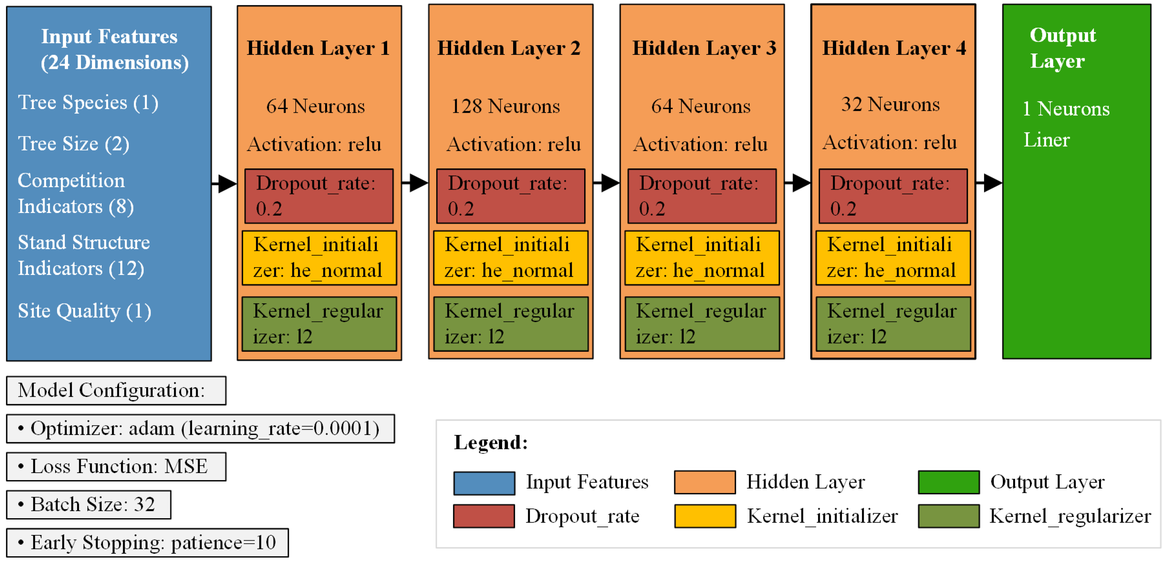
The performance and convergence of the DNN model are affected by a variety of factors, mainly including the number of hidden layers, the number of neurons in each hidden layer, loss functions, regularization methods, initialization schemes, optimization algorithms, learning rate, activation functions, training epochs, batch size, epoch, etc. [4,49,53]. The structure of the DNN with input variables for tree CW prediction is shown in Figure 2.
We implemented a four-tiered hyperparameter optimization framework with progressively increasing complexity: (1) Base architecture: 2–5 hidden layers with neurons per layer in 2n (n = 0 to 8), namely [1, 2, 4, 8, 16, 32, 64, 128, 256]. (2) Data-scaled architecture: 2–5 layers with neuron counts scaled to input feature dimensionality, establishing a direct relationship between data complexity and model capacity. (3) Regularized scaling: configuration (2) + L2 regularization + dropout, enhancing generalization capability and mitigate overfitting. (4) Full optimization: configuration (3) + kernel initializer selection + optimizer tuning + learning rate adjustment + activation function choice, representing the most sophisticated level of architectural refinement. Specific hyperparameter configurations are detailed in Table 2.
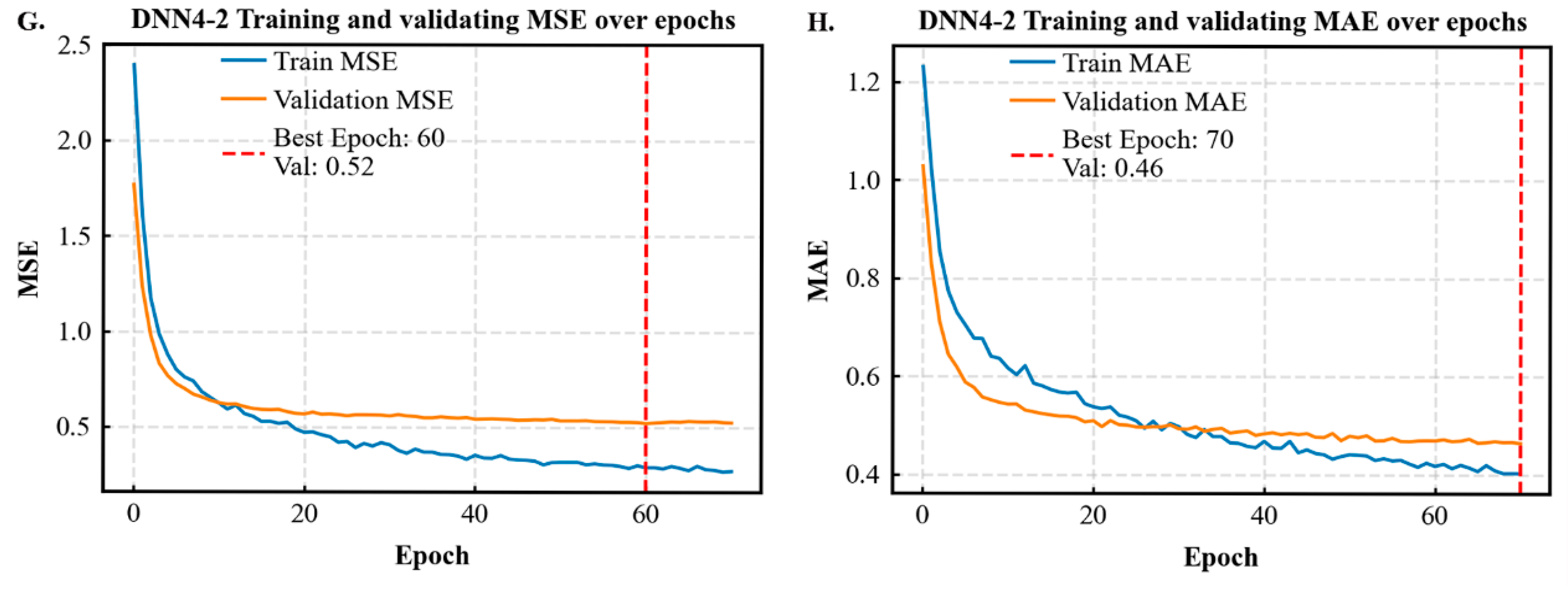
The number of training epochs was set at 300 for all DNN models to achieve optimal performance [16]. The values of other hyperparameters adopted the default settings of the optimizer. “max_trials” was set to 200. Random_state was set to 42. Additionally, an early stop function with a patience value of 10 was used to stop training when a monitored metric has stopped improving (min_delta = 0.0001). The optimal number of training epochs was determined by identifying the Pareto-optimal balance between MSE and MAE values on both training and validation sets. All DNN model trainings in our study were conducted using Tensor Flow 2.10, Keras Tuner 1.1.2, and Numpy 1.23.5 in Python 3.9 [54]. The models were executed on the following hardware environment: CPU: 12th Gen Intel(R) Core(TM) i7-12700KF 3.60 GHz; RAM: 32.0 GB; System Type: 64-bit operating system, x64-based processor. Without using mixed precision or GPU acceleration, restore_festw_weights were used together with early stop. Bayesian Optimization was employed to find hyperparameters for the DNN models.

2.3. Input Variables

Considering the primary factors influencing tree growth, this study selected input variables that represented a set of key factors, namely tree species, tree size, competition indicators, stand structural indicators, and site quality. In the natural secondary forests studied, Larix principis-rupprechtii and Picea asperata constituted the dominant species. Categorical species variables underwent one-hot encoding method [16]. Tree size was quantified by DBH and H. Competition indicators included: (1) Stand density: stems per hectare (N), stand density index (SDI); (2) Basal area: basal area per hectare (BA); (3) Size distribution: quadratic mean DBH (Dg); (4) Neighborhood competition: tree-level (Utree) and stand-level (Ustand) [55]; (5) Spatial crowding: tree concentration index (Ctree) and stand mean concentration (Cstand). Stand structure indicators comprised: (1) Size heterogeneity: gini coefficient (GC), DBH coefficient of variation (CVd); (2) Diversity indices: 1-D and H′; (3) Spatial patterns: neighborhood configuration: tree (Wtree) and stand (Wstand) patterns, Species mingling: tree (Mtree) and stand mean (Mstand) indices, Spatial arrangement: Clark-Evans aggregation index (R); (4) Canopy structure: maximum DBH (Dmax), stand crowding index (K), and arithmetic mean height ( H ¯ ). Site quality was represented by HD. Given substantial heterogeneity in CW predictors, all numerical variables were standardized to accelerate model convergence [16,24,55].
In order to explore the construction methods of competition and stand structure indicators related to tree growth in complex natural secondary forests, considering the practical situation of adjacent tree interactions, this study constructed partial competition and stand structure indicators (1-D, H′, Wstand, R, CVd, K, Ustand, GC, and Cstand) in two ways: (1) The first method considered all live trees; (2) The HTM, removed live trees with a height of less than 15 m (they may have little impact on the target tree and stand environment, and the size of this value was determined by the height from the ground to the base of the main live crown) and used the remaining live trees (H ≥ 15 m) for the statistical calculation of stand factors. The choice was operationally defined based on the key ecological principle of focusing on trees within the main canopy layer that are most likely to engage in direct light competition and exert significant influence on the target tree’s crown development. The construction of the remaining variables was carried out using all the live trees.
We systematically evaluated the four DNN architectures (DNN1, DNN2, DNN3, and DNN4) using two groups of input variables as defined in our experimental design. Each model underwent comprehensive training, validation, and performance assessment with both variable groups independently, enabling direct comparison of their predictive capabilities across different feature combinations. The detailed combinations of input variables for all models are presented in Table 3.

2.4. Model Evaluation and Validation

We implemented a structured cross-validation protocol with plot-level partitioning to ensure robust model evaluation. The entire dataset was first stratified by forest type and site conditions, then randomly partitioned at the plot level into training (70%), validation (10%), and testing (20%) subsets. This plot-level partitioning prevented data leakage by ensuring that trees from the same plot remained within the same data split. A ten-fold cross-validation scheme was subsequently applied to the training dataset, where folds were created by randomly assigning entire plots to different folds while maintaining the original distribution of CW measurements. In each cross-validation iteration, the model was trained on nine folds, validated on one fold for hyperparameter tuning, and the process was repeated until all folds had served as the validation set. The final model performance was assessed on the completely held-out testing subset.
The R2, MSE, MAE, and MAPE were selected to evaluate the model performance (Equations (1)–(4)):
R 2 = 1 i = 1 m j = 1 n CW i j CW i j ^ 2 i = 1 m j = 1 n CW i j CW i j ¯ 2
MSE = 1 2 N i = 1 m j = 1 n CW i j CW i j ^ 2
MAE = i = 1 m j = 1 n CW i j CW i j ^ N
MAPE = i = 1 m j = 1 n CW i j CW i j ^ CW i j × 100 % N
where m represents the number of subplots; n represents the number of trees per subplots; CWij represents the CW of the j-th tree within the i-th subplot, CW i j ^ represents the predicted value of CW, and CW i j ¯ represents the average value of CW; N represents the total number of trees.
This study employed the scipy.stats.normaltest (residuals) function from the SciPy library to conduct the D’Agostino–Pearson normality test (α = 0.05) for assessing the normality of the residuals [56].

2.5. Variable-Importance Methodology and Feature Selection

The feature selection methodology employed a two-stage approach. First, we performed initial feature screening using Pearson correlation coefficients to identify variables with strong linear relationships to CW. The top 15 variables were selected based on the highest absolute correlation values from this analysis.

3. Results

3.1. Performance of Various Models for Predicting Tree CW

Statistical metrics for both training and validation folds during 10-fold cross-validation across all models are presented in Table 4. Results indicate no significant overfitting occurred, demonstrating stable model performance. For Dataset 1’s validation set, R2 exhibited a decline-then-increase trend with rising model complexity, peaking at DNN4-1 (R2 = 0.69 ± 0.04). Dataset 2’s validation R2 followed an identical trend, reaching its maximum at DNN4-2 (R2 = 0.71 ± 0.04). Conversely, MSE, MAE, and MAPE for Dataset 1’s validation set showed an increase-then-decrease pattern. For Dataset 2, these three error metrics displayed an overall decreasing trend.
Training curves for all models on Dataset 1 and Dataset 2 are presented in Figure 3 and Figure 4, respectively. Results demonstrate decreasing MSE and MAE values on both training and validation sets as epochs progress. Most curves exhibit rapid declines before approximately epoch 10, followed by gradual plateaus. For Dataset 1, optimal epochs determined by MSE and MAE show minor discrepancies in DNN1-1 and DNN2-1, but significant divergence in DNN3-1 and DNN4-1. Conversely, Dataset 2 displays consistent epoch convergence across all models (DNN1-2 to DNN4-2) when optimized via MSE versus MAE criteria.
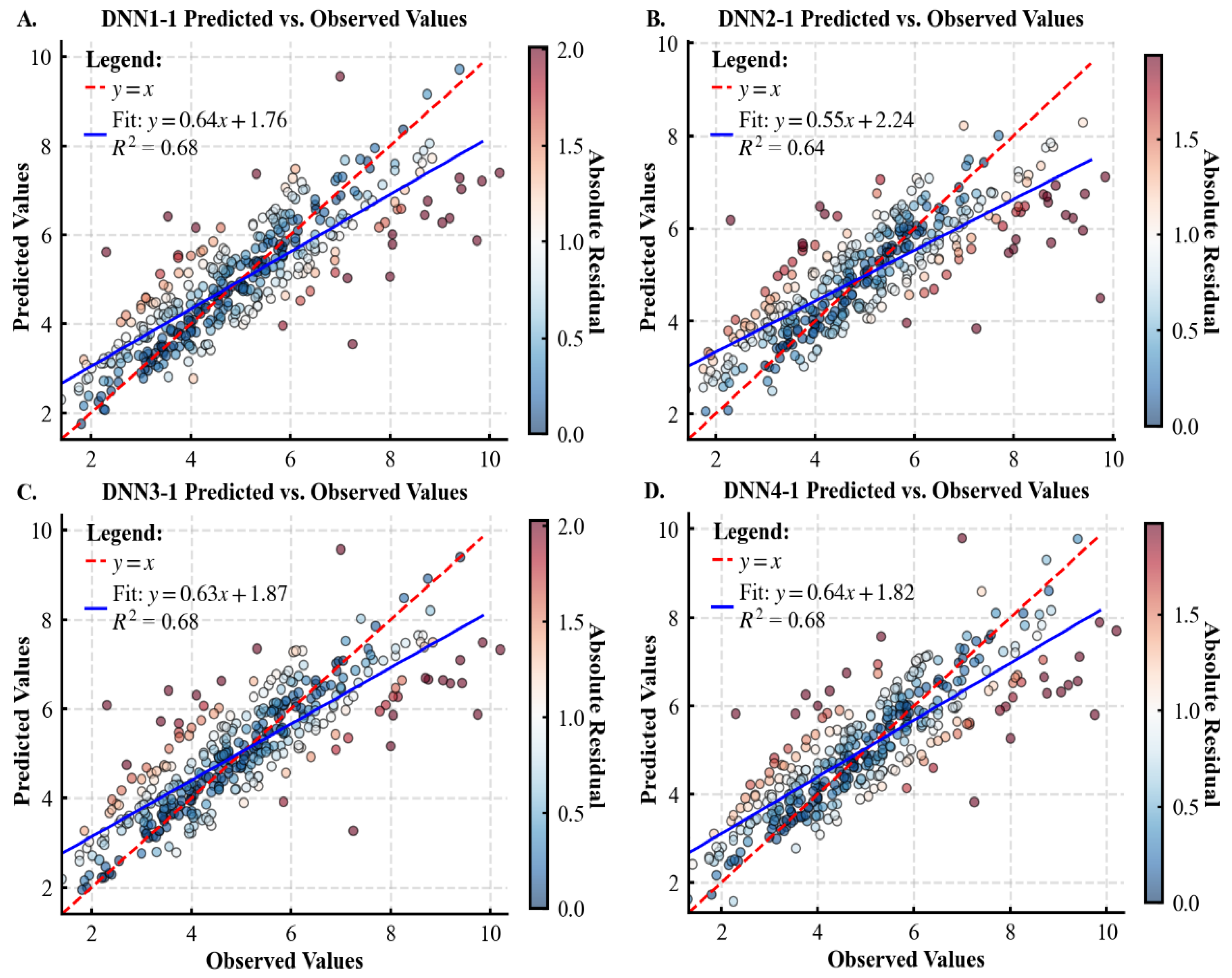
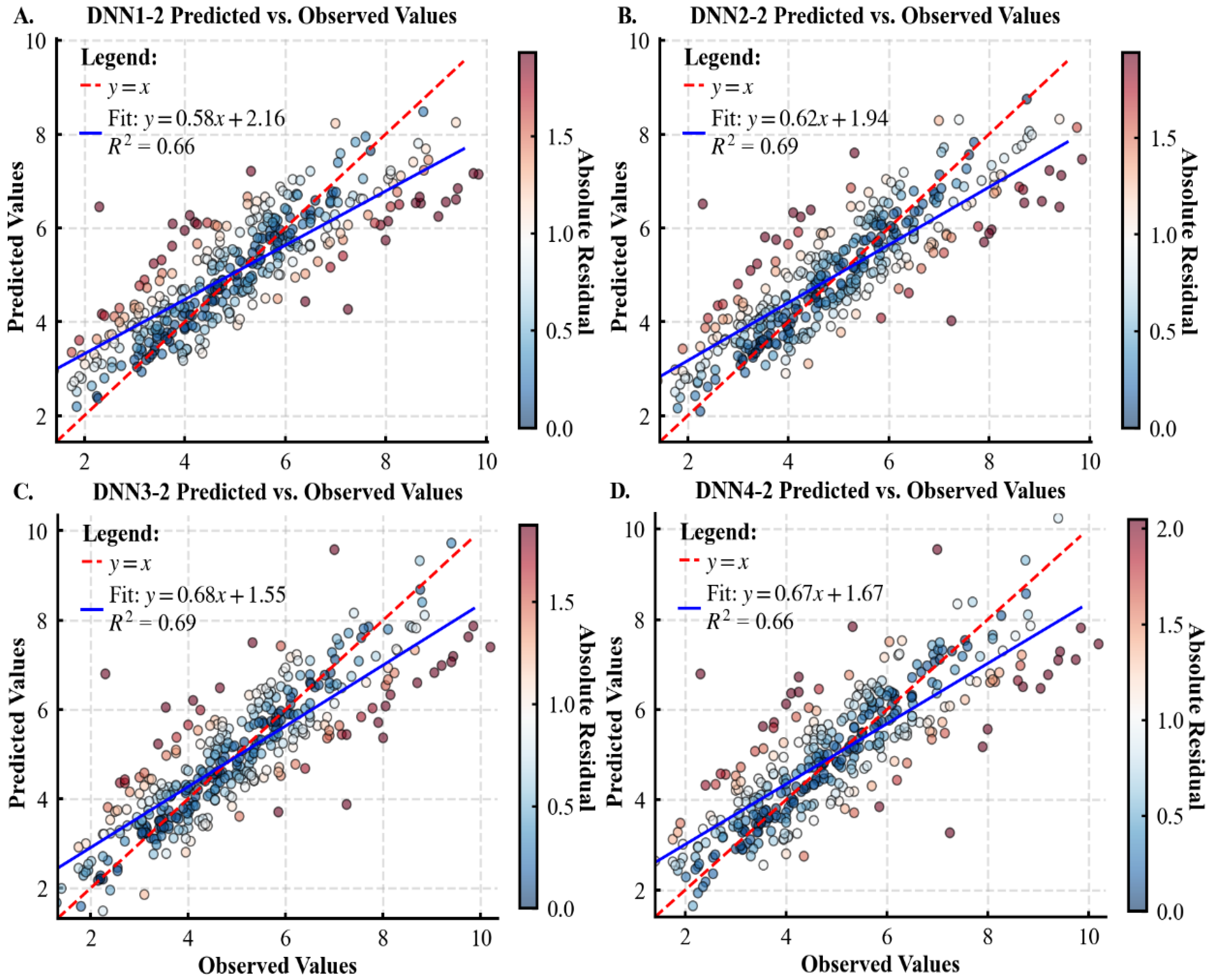
Relationships between predicted and observed values on the test sets of Datasets 1 and 2 are shown in Figure 5 and Figure 6, respectively. For Dataset 1, the slope of the linear regression between predictions and observations demonstrated a concave trend (decrease followed by increase) with rising model complexity. DNN1-1 and DNN4-1 achieved the maximum slope (0.64) and R2 (0.68), while DNN2-1 yielded the minimum slope (0.55) and R2 (0.64). Conversely, Dataset 2 exhibited a convex trend (increase then decrease) in both slope and R2. Here, DNN3-2 attained peak performance (slope = 0.68, R2 = 0.69), whereas DNN1-2 showed the lowest values (slope = 0.58, R2 = 0.66).
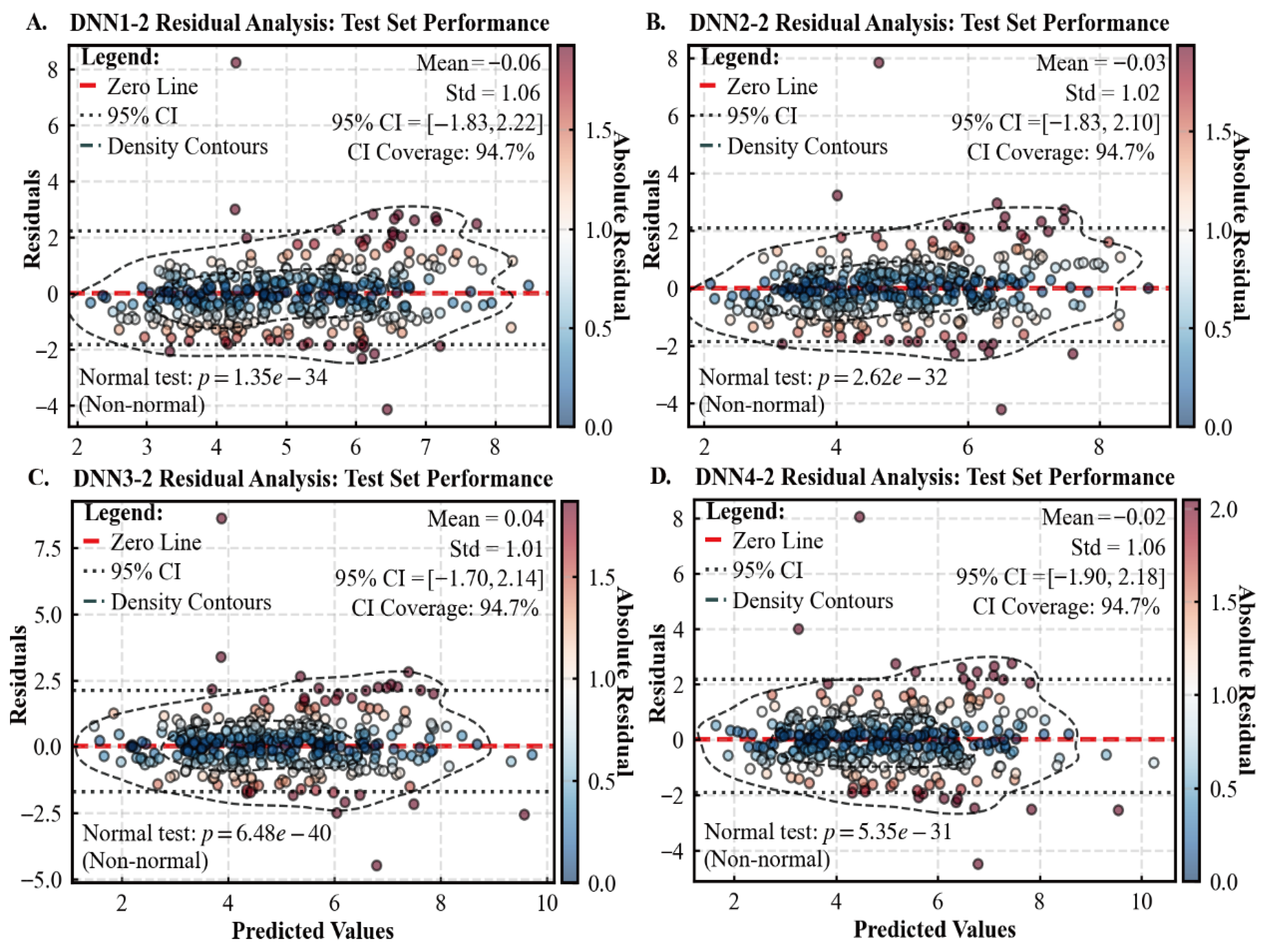
Residual plots for test sets of Datasets 1 and 2 are presented in Figure 7 and Figure 8, respectively. Both datasets demonstrated: 94.7% CI coverage across all models (approximating the nominal 95% level).
Mean residuals near zero, ranging between −0.06 m and 0.04 m. Non-normally distributed residuals (D’Agostino–Pearson normality test, p < 0.001). For Dataset 1, DNN1-1 and DNN4-1 exhibited is density lines closest to bivariate normal ellipses. In Dataset 2, DNN3-2 showed the best approximation to elliptical contours.

3.2. Effect of Different Input Variables on Tree CW Prediction

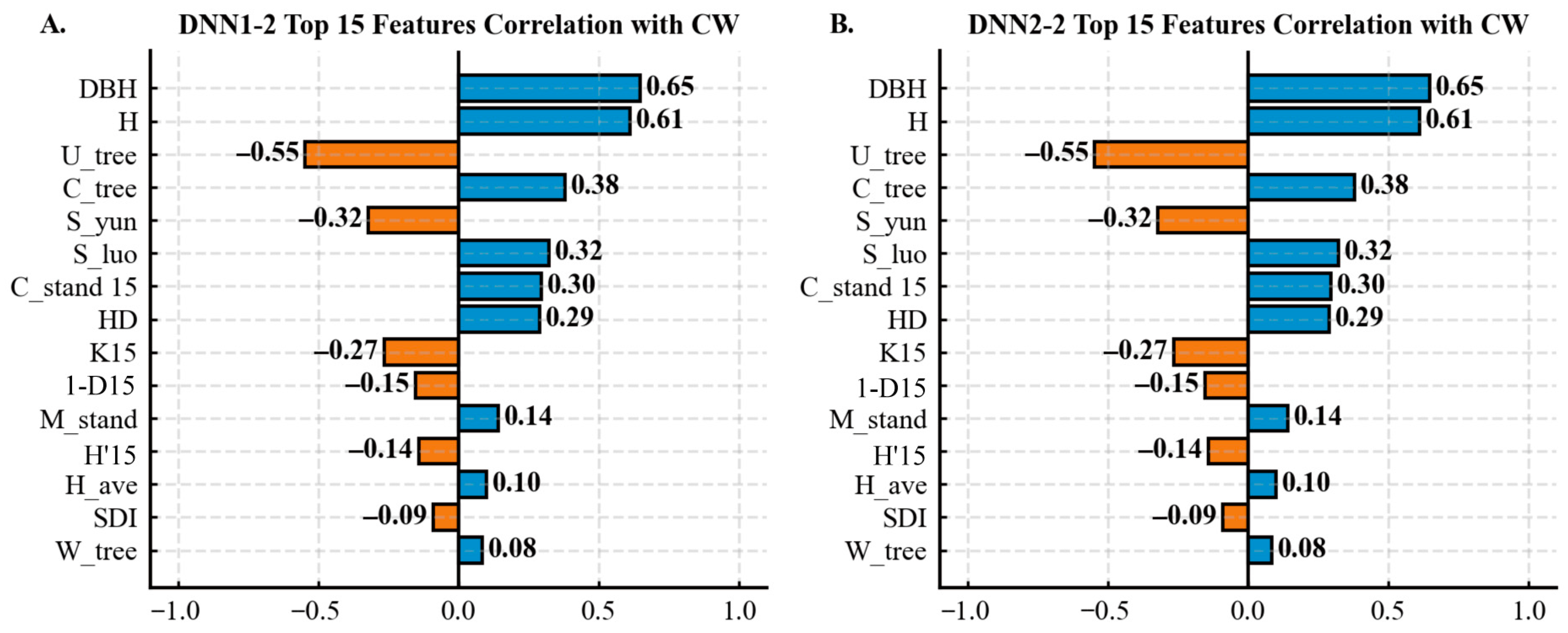
Variable importance rankings for Datasets 1 and 2 are presented in Figure 9 and Figure 10, respectively. Within Dataset 1, both the identities and importance values of the top 15 variables showed perfect consistency across all models. Similarly, Dataset 2 exhibited complete agreement in the top 15 variables and their importance rankings among models. When comparing across datasets, the six most influential variables maintained identical identity, ranking order, and importance values: DBH (0.65), H (0.61), U_tree (−0.55), C_tree (0.38), S_yun (−0.32), and S_luo (0.32). However, C_stand ascended from rank 9 (importance: +0.22) in Dataset 1 to rank 7 (+0.30) in Dataset 2. HD declined from rank 7 (+0.29) to rank 8 (+0.29). K dropped from rank 8 (−0.26) to rank 9 while showing marginally increased importance (−0.27). H’ declined from rank 10 (+0.15) to rank 12 with reversed directionality (−0.14). Conversely, 1-D rose from rank 12 (+0.13) to rank 10 while exhibiting opposite effects (−0.15).

4. Discussion

4.1. Deep Learning Algorithm for Tree CW Prediction

Despite numerous existing methods, including basic DNN models, having been applied to CW prediction [16,17,20,33,39], our study presents the first investigation of DNNs with varied architectural complexity for CW estimation in natural secondary forests dominated by Larix principis-rupprechtii and Picea asperata in Northern China. We developed and evaluated eight distinct DNN configurations through systematic combinations of four complexity levels and two variable sets. Comprehensive validation identified the DNN3-2 model as the optimal architecture, explaining 69% of CW variance without significant heteroskedasticity.
Hyperparameter tuning remains a core challenge in neural-network modeling [53,57]. Model performance is depends critically on optimal hyperparameter configuration, including architecture (hidden layers and neuron counts), loss functions, regularization methods, initialization schemes, optimization algorithms, learning rates, activation functions, and training epochs [49,53]. Although manual and grid searches are still widely used [58,59], their computational costs become prohibitive as complexity of hyperparameter spaces expand [57]. This limitation has driven the development of efficient alternatives, including Random Search [58], Bayesian Optimization [57,60], Population-Based Training [61], Hyperband Optimization [62], and Genetic Algorithm [57]. We employed well-established Bayesian Optimization, a probabilistic model-based approach for global efficiency [57,60,63]. This methodology intelligently selects the most promising hyperparameter combinations for evaluation using acquisition functions, substantially reducing evaluations required for convergence. Implemented with the BayesianOptimization package in Python, the procedure converged systematically on the optimal hyperparameter set.
Divergent perspectives exist regarding optimal hidden layer neuron configuration. Some studies advocate neuron counts exceeding twice the input layer dimensionality [64,65], while others contend that hidden layer architecture should be entirely data-scale dependent [66,67]. Building upon prior methodologies [45,68,69] and considering our research objectives, computational constraints, and deep learning domain expertise, we implemented a four-tiered hyperparameter optimization framework: (1) Base architecture: 2-5 hidden layers with neurons per layer in 2n (n = 0 to 8); (2) Data-scaled architecture: 2–5 layers with neuron counts scaled to input feature dimensionality; (3) Regularized scaling: configuration (2) + L2 regularization + dropout; (4) Full optimization: configuration (3) + kernel initializer selection + optimizer tuning + learning rate adjustment + activation function choice. This framework progressively incorporates greater hyperparameter sophistication with increasing complexity levels.
To avoid overfitting, we employed the early-stopping technique [41,70] during DNN training. All DNN models in this study exhibited no overfitting (Table 4, Figure 3 and Figure 4). The bias-variance trade-off represents a fundamental challenge in training DNN models [71,72]. When model complexity increases and training epochs accumulate, the continuous gradual decline in training loss may paradoxically weaken generalization performance [73,74]. To comprehensively evaluate the persistent decrease in training loss and identify the corresponding optimal epoch count, training was terminated when the reduction in MSE and MAE on both training and validation sets became no longer significant. For the first time, the Pareto optimality method was adopted to holistically determine the optimal stopping epoch.

4.2. Contributions of Important Input Variables to CW Prediction

Accurate estimation of CW highly depends on the type and variety of input variables, primarily including tree dimensions (DBH and H), species, site quality, stand structure, climatic conditions, and other factors [17,75]. In our models, DBH was the most influential predictor (importance value: 0.65), followed by tree height (H, importance value: 0.61), consistent with previous research [17,21,76]. Our results ranked the competition indices Utree and Ctree (representing neighbor tree relationships) as the third and fourth most important variables (Figure 9 and Figure 10), indicating that inter-tree competition significantly influences crown width. The forest stand in this study is currently in the middle-aged stage, a critical and dynamic period during forest development. During this stage, tree crowns continue to expand, leading to a sharply increasing demand for space and resources. Intensified competition among individual trees causes the crowns of some suppressed trees to begin shrinking. Furthermore, both intraspecific and interspecific competition result in the gradual die-off of numerous underperforming trees, primarily those in a suppressed state. Notably, Utree exhibited a negative effect on CW, while Ctree had a positive effect. The negative effect of Utree suggests competitive inhibition of crown development by neighboring trees. Conversely, the positive effect of Ctree implies that denser neighbor structures may promote crown growth, potentially attributable to the complex stand structure, high tree heterogeneity, and strong complementarity in resource utilization within natural forests [4,24,77].
We employed one-hot encoding to process tree species categorical variables in the DNN models, revealing the mechanism of species influence on crown width prediction [4,78]. The species indicators Syun and Sluo were ranked fifth and sixth in importance (Figure 9 and Figure 10), confirming the significant role of tree species on crown development [24,77,79]. In natural mixed forests, interspecific genetic differences, stand structural complexity, and spatial heterogeneity lead to divergence in light absorption capacity and competitiveness, resulting in interspecific crown width variation [14,24,79].
Site quality can be characterized by metrics such as HD [17,80,81], site index [82], and topographic factors (elevation, slope, aspect) [19]. Our results showed HD consistently ranked relatively high (seventh or eighth) across all models (Figure 9 and Figure 10), confirming the importance of site quality for CW prediction and demonstrating the reasonable coverage of site conditions in our plot design. These variables reflect a tree’s competitive status for environmental resources, governing growth processes and crown recession [24,83]. Due to spatial scale constraints, climatic factors were not validated in this study [24].
Compared with structurally uniform plantations, natural forests exhibit complex and diverse stand structures with high heterogeneity [24,37]. Consequently, methods for calculating stand structural parameters from the structural units of neighboring trees should differ between these two forest types. Our novel HTM significantly enhanced the calculation of neighbor-based stand structural parameters in these complex forest ecosystems, which concurrently improved CW prediction accuracy, and strengthened the interpretability of key variable effects. The results demonstrate that among all nine indicators (Ustand, Cstand, GC, 1-D, H′, Wstand, R, CVd, K) calculated using the HTM proposed in this study, four (Cstand, 1-D, H′, K) were included in the top 15 most important variables (Figure 9). When comparing the top 15 variables between Dataset 1 and Dataset 2, Cstand15 exhibited the most significant change in importance and surpassed HD (representing site quality) in predictive weight. This indicates that methodological differences in calculating stand structural parameters based on neighboring tree units substantially impact CW prediction, suggesting that the newly calculated indicators better characterize stand conditions. Notably, H15 and 1-D15 (derived from H′ and 1-D via the HTM) exhibited divergent effects on CW prediction. This phenomenon may stem from the processing steps of the HTM, which filters out trees not reaching the main canopy layer, retaining only those trees within the main canopy where crowns directly interact. Crucially, DNN models consistently outperformed on Dataset 2 compared to Dataset 1 during both training (Table 4) and testing phases (Figure 5, Figure 6, Figure 7 and Figure 8). This validates the theoretical and practical significance of the HTM proposed in this study.

5. Conclusions

This study developed four progressively complex DNN models to accurately predict individual-tree CW in complex natural mixed forests of Northern China, dominated by Larix principis-rupprechtii and Picea asperata. A key contribution was the introduction of an HTM, which significantly improved the computation of neighborhood-based stand structural parameters. The HTM not only enhanced CW prediction accuracy but also increased the interpretability of key ecological variables.
We found that while increasing model complexity moderately improved predictions, the integration of biologically meaningful variables had a greater impact on performance than further architectural refinement. This underscores the importance of ecologically informed feature selection in modeling complex forest systems. Key predictors of CW included tree dimensional attributes, neighborhood competition, species composition, and site quality. Among the architectures tested, the DNN3-2 model—with its optimized hidden layer structure, neuron density, L2 regularization, and dropout hyperparameters—was identified as the most effective. The combination of a structured DNN and the HTM provides a robust framework for predicting individual tree CW in mixed-species natural forests.
Despite these findings, this study has several limitations that point to critical avenues for future research. First, the fixed 15 m threshold employed in the HTM requires further sensitivity analysis to establish a standardized, ecologically grounded methodology for threshold selection. More importantly, the model’s generalizability could be substantially enhanced by integrating key environmental and temporal drivers not included in the current framework. We specifically identify three pivotal directions for subsequent investigations: (1) the integration of climatic variables to account for their influence on growth processes; (2) the incorporation of dendrochronological (tree-ring) data to understand the temporal dynamics of crown development in relation to tree age and stand developmental stage; and (3) the expansion of the database to encompass a wider range of forest types, age classes, and site conditions. Addressing these limitations will be crucial for developing more robust, universally applicable, and temporally sensitive models of crown morphology.

Author Contributions

Conceptualization, L.Z. and X.C.; methodology, L.Z.; software, L.Z.; validation, L.Z., S.L., and W.P.; formal analysis, W.P.; investigation, L.Z., X.C., S.L., C.H., W.P., and M.Z.; resources, L.Z.; data curation, X.C. and C.H.; writing—original draft preparation, L.Z.; writing—review and editing, W.P.; visualization, L.Z.; supervision, M.Z.; project administration, L.Z.; funding acquisition, L.Z. All authors have read and agreed to the published version of the manuscript.

Funding

This research was funded by the Shanxi Basic Research Program Project, grant number 202303021222073.

Data Availability Statement

The datasets used in this study are available from the corresponding author on reasonable request.

Acknowledgments

We thank the handing editor and anonymous reviewers for their valuable comments.

Conflicts of Interest

The authors declare that they have no known competing financial interests, or personal relationships that could have appeared to influence the work reported in this paper.

Abbreviations

The following abbreviations are used in this manuscript:
CWCrown width. It represents the horizontal area of influence for a tree, measured through perpendicular crown spread diameters to assess light interception and growing space.
DNNDeep neural network. A DNN is a multi-layered computational model that learns hierarchical patterns from data through backpropagation, capable of approximating complex functions for regression and classification tasks.
LMELinear mixed-effects models. LME models are statistical approaches that incorporate both fixed effects to estimate population-level parameters and random effects to account for variability from grouped or hierarchical data structures.
NSURNonlinear seemingly unrelated regression. NLSUR is an econometric technique that simultaneously estimates a system of nonlinear equations with correlated error terms, thereby improving efficiency by accounting for cross-equation dependencies in the stochastic components.
GAMGeneralized additive model. A GAM is a statistical framework that extends generalized linear models by incorporating smooth, non-parametric functions of predictors to capture complex nonlinear relationships while maintaining interpretability through its additive structure.
NLMENonlinear mixed effects models. NLME is hierarchical statistical framework that incorporate both fixed effects describing population-average nonlinear relationships and random effects accounting for individual-specific variations in these nonlinear patterns across grouped or longitudinal data.
GNLMEGeneralized nonlinear mixed effects models. A GNLME is a comprehensive statistical framework that integrates the flexibility of nonlinear mean structures, the capacity to handle non-normal response distributions through link functions, and the ability to account for between-subject variability through random effects in hierarchical data.
DLADeep learning algorithms. DLA is a class of machine learning method that utilize multi-layered neural networks with hierarchical feature learning capabilities to automatically extract complex patterns and representations from raw data through successive nonlinear transformations.
CNNConvolutional neural network. A CNN is a specialized deep learning architecture that employs convolutional filters to automatically and adaptively learn spatial hierarchies of features through backpropagation, making it particularly effective for processing grid-like data such as images and time series.
RNNRecurrent neural network. A RNN is a class of artificial neural networks designed to process sequential data by maintaining internal memory through cyclic connections, enabling temporal dynamic behavior and modeling of dependencies across time steps.
DBHDiameter at breast height. DBH is a standard forestry measurement of tree trunk diameter, typically taken at 1.3 m (4.5 feet) above ground level, serving as a fundamental metric for estimating tree volume, growth, and biomass.
HTotal height. H is a fundamental tree dimension metric representing the vertical distance from the ground level (or root collar) to the highest point of the tree crown, typically measured using clinometers, hypsometers, or laser rangefinders in forest inventory and ecological studies.
NStems per hectare. N is a fundamental forest density metric quantifying the number of individual tree stems within a one-hectare area, serving as a crucial measure for assessing stand stocking, competition intensity, and silvicultural treatment requirements.
SDIStand density index. SDI is a dimensionless measure of stand crowding that quantifies the number of trees per unit area relative to a standard reference diameter.
BABasal area per hectare. BA is a fundamental metric of stand density that represents the total cross-sectional area of all tree stems measured at breast height (1.3 m) contained within one hectare, providing a comprehensive measure of space occupancy and growing stock in forest ecosystems.
DgQuadratic mean DBH. Dg is a stand-level metric calculated as the diameter of the tree of average basal area, derived by squaring individual tree DBHs, computing their arithmetic mean, and then taking the square root, providing a biologically meaningful representation of central tendency in forest stands.
USize ratio. It quantifies the relative dimensional relationship between a subject tree and its competitors, typically calculated as the diameter ratio (DBHj/DBHi) to assess competitive asymmetry within a forest stand.
CConcentration index. C is a statistical measure that quantifies the degree of inequality or clustering in the distribution of resources, individuals, or events within a defined population or geographical area, typically ranging from 0 (perfect equality) to 1 (maximum concentration).
GCGini coefficient. The GC is a statistical measure of distributional inequality that quantifies the degree of disparity within a given population, ranging from 0 (perfect equality) to 1 (maximum inequality), and is most commonly applied to evaluate income or wealth distribution patterns in economic and social systems.
CVdDBH coefficient of variation. The CVd quantifies the relative variability of tree diameters within a forest stand by expressing the standard deviation of DBH measurements as a percentage of the mean DBH, serving as a key indicator of structural diversity and size inequality in even-aged and uneven-aged stands.
1-DSimpson’s index. One-dimensional quantifies the probability that two randomly selected individuals from a community will belong to different species, thereby integrating both species richness and abundance evenness into a unified measure of ecological diversity.
HShannon’s index. H′ quantifies ecological diversity by measuring the uncertainty in predicting the species of a randomly selected individual from a community, integrating both species richness and evenness through a logarithmic weighting of relative abundances.
WNeighborhood configuration. W refers to the spatial arrangement, structural composition, and competitive interactions among trees within a defined area surrounding a subject tree, typically quantified through distance-dependent and size-based metrics to assess local competition intensity and resource availability in forest stands.
MSpecies mingling. M quantifies the spatial diversity of tree species by measuring the proportion of nearest neighbors that differ in species from a focal tree, thereby evaluating the fine-scale spatial intimacy and mixture patterns among species within a forest stand.
RClark-Evans aggregation index. The R is a spatial point pattern statistic that quantifies the degree of clustering or dispersion in plant populations by comparing the observed mean distance to nearest neighbors with the expected mean distance under a completely random spatial distribution.
DmaxMaximum DBH. Dmax is the largest diameter at breast height (1.3 m above ground) recorded among all living trees within a defined forest stand or sampling area, serving as a critical indicator of stand maturity, site productivity potential, and structural complexity in forest ecosystems.
KStand crowding index. K quantifies the level of competition for resources within a forest stand by integrating tree density, size distribution, and spatial arrangement, typically expressed as a relative measure comparing actual stand conditions to a reference density for optimal growth.
H ¯ Arithmetic mean height. H ¯ is a stand-level metric calculated as the simple average of individual tree heights within a defined forest area, obtained by summing all measured tree heights and dividing by the total number of trees, providing a straightforward representation of the central tendency in vertical stand structure.
HDMean dominant height. HD is a fundamental forest mensuration parameter representing the average height of the most vigorous trees in a stand—typically defined as the 100 thickest trees per hectare—which serves as a reliable indicator of site productivity potential and is widely used for forest site classification and growth modeling.
R2Coefficient of determination. The R2 quantifies the proportion of variance in the dependent variable that is predictable from the independent variable(s) in a regression model, serving as a fundamental metric for assessing model fit and explanatory power.
MSEMean square error. MSE is a fundamental regression metric that quantifies prediction accuracy by calculating the average squared difference between observed and predicted values, thereby emphasizing larger errors through its quadratic penalty term.
MAEMean absolute error. MAE is a robust regression metric that measures the average magnitude of prediction errors by calculating the arithmetic mean of absolute differences between observed and predicted values, providing an interpretable measure of average model accuracy in the original units of the response variable.
MAPEMean absolute percentage error. MAPE is a relative accuracy metric that measures the average magnitude of prediction errors expressed as percentages of the actual observed values, calculated as the mean of absolute percentage differences between predicted and true values across all observations.

References

  1. Crous, K.Y.; Campany, C.; Lopez, R.; Cano, F.J.; Ellsworth, D.S. Canopy position affects photosynthesis and anatomy in mature Eucalyptus trees in elevated CO2. Tree Physiol. 2021, 41, 206–222. [Google Scholar] [CrossRef]
  2. Li, Y.; Su, Y.; Zhao, X.; Yang, M.; Hu, T.; Zhang, J.; Liu, J.; Liu, M.; Guo, Q. Retrieval of tree branch architecture attributes from terrestrial laser scan data using a Laplacian algorithm. Agric. For. Meteorol. 2020, 284, 107874. [Google Scholar] [CrossRef]
  3. Shenkin, A.; Bentley, L.P.; Oliveras, I.; Salinas, N.; Adu-Bredu, S.; Marimon-Junior, B.H.; Marimon, B.S.; Peprah, T.; Choque, E.L.; Rodriguez, L.T.; et al. The influence of ecosystem and phylogeny on tropical tree crown size and shape. Front. For. Glob. Change 2020, 3, 501757. [Google Scholar] [CrossRef]
  4. Qin, Y.; He, X.; Lei, X.; Feng, L.; Zhou, Z.; Lu, J. Tree size inequality and competition effects on nonlinear mixed effects crown width model for natural spruce-fir-broadleaf mixed forest in northeast China. For. Ecol. Manag. 2022, 518, 120291. [Google Scholar] [CrossRef]
  5. Li, X.; Yang, X.; Dong, B.; Liu, Q. Predicting 28-day all-cause mortality in patients admitted to intensive care units with pre-existing chronic heart failure using the stress hyperglycemia ratio: A machine learning-driven retrospective cohort analysis. Cardiovasc. Diabetol. 2025, 24, 10. [Google Scholar] [CrossRef]
  6. Sapijanskas, J.; Paquette, A.; Potvin, C.; Kunert, N.; Loreau, M. Tropical tree diversity enhances light capture through crown plasticity and spatial and temporal niche differences. Ecology 2014, 95, 2479–2492. [Google Scholar] [CrossRef]
  7. Pretzsch, H. Tree growth as affected by stem and crown structure. Trees 2021, 35, 947–960. [Google Scholar] [CrossRef]
  8. Krajnc, L.; Farrelly, N.; Harte, A. The influence of crown and stem characteristics on timber quality in softwoods. For. Ecol. Manag. 2019, 435, 8–17. [Google Scholar] [CrossRef]
  9. Fang, S.; Liu, Y.; Yue, J.; Tian, Y.; Xu, X. Assessments of growth performance, crown structure, stem form and wood property of introduced poplar clones: Results from a long-term field experiment at a lowland site. For. Ecol. Manag. 2021, 479, 118586. [Google Scholar] [CrossRef]
  10. Liang, R.; Sun, Y.; Zhou, L.; Wang, Y.; Qiu, S.; Sun, Z. Analysis of various crown variables on stem form for Cunninghamia lanceolata based on ANN and taper function. For. Ecol. Manag. 2022, 507, 119973. [Google Scholar] [CrossRef]
  11. Liu, X.; Su, Y.; Hu, T.; Yang, Q.; Liu, B.; Deng, Y.; Tang, H.; Tang, Z.; Fang, J.; Guo, Q. Neural network guided interpolation for mapping canopy height of China’s forests by integrating GEDI and ICESat-2 data. Remote Sens. Environ. 2022, 269, 112844. [Google Scholar] [CrossRef]
  12. Rahman, M.F.; Onoda, Y.; Kitajima, K. Forest canopy height variation in relation to topography and forest types in central Japan with LiDAR. For. Ecol. Manag. 2022, 503, 119792. [Google Scholar] [CrossRef]
  13. Sun, Y.; Gao, H.; Li, F. Using linear mixed-effects models with quantile regression to simulate the crown profile of planted Pinus sylvestris var. Mongolica trees. Forests 2017, 8, 446. [Google Scholar] [CrossRef]
  14. Zhou, Z.; Fu, L.; Zhou, C.; Sharma, R.P.; Zhang, H. Simultaneous compatible system of models of height, crown length, and height to crown base for natural secondary forests of Northeast China. Forests 2022, 13, 148. [Google Scholar] [CrossRef]
  15. Ma, A.; Miao, Z.; Xie, L.; Dong, L.; Li, F. Crown width prediction for Larix olgensis plantations in Northeast China based on nonlinear mixed-effects model and quantile regression. Trees 2022, 36, 1761–1776. [Google Scholar] [CrossRef]
  16. Qin, Y.; Wu, B.; Lei, X.; Feng, L. Prediction of tree crown width in natural mixed forests using deep learning algorithm. For. Ecosyst. 2023, 10, 100109. [Google Scholar] [CrossRef]
  17. Sharma, R.P.; Bílek, L.; Vacek, Z.; Vacek, S. Modelling crown width-diameter relationship for Scots pine in the central Europe. Trees 2017, 31, 1875–1889. [Google Scholar] [CrossRef]
  18. Jia, W.; Chen, D. Nonlinear mixed-effects height to crown base and crown length dynamic models using the branch mortality technique for a Korean larch (Larix olgensis) plantations in northeast China. J. For. Res. 2019, 30, 2095–2109. [Google Scholar] [CrossRef]
  19. Buchacher, R.; Ledermann, T. Interregional crown width models for individual trees growing in pure and mixed stands in Austria. Forests 2020, 11, 114. [Google Scholar] [CrossRef]
  20. Raptis, D.I.; Kazana, V.; Kechagioglou, S.; Kazaklis, A.; Stamatiou, C.; Papadopoulou, D.; Tsitsoni, T. Nonlinear Quantile Mixed-Effects Models for Prediction of the Maximum Crown Width Fagus sylvatica L., Pinus nigra Arn. and Pinus brutia Ten. Forests 2022, 13, 499. [Google Scholar] [CrossRef]
  21. Qiu, S.; Gao, P.; Pan, L.; Zhou, L.; Liang, R.; Sun, Y.; Wang, Y. Developing nonlinear additive tree crown width models based on decomposed competition index and tree variables. J. For. Res. 2023, 34, 1407–1422. [Google Scholar] [CrossRef]
  22. Wang, J.; Jiang, L.; Xin, S.; Wang, Y.; He, P.; Yan, Y. Two new methods applied to crown width additive models: A case study for three tree species in Northeastern China. Ann. For. Sci. 2023, 80, 11. [Google Scholar] [CrossRef]
  23. Zhou, X.; Li, Z.; Liu, L.; Sharma, R.P.; Guan, F.; Fan, S. Constructing two-level nonlinear mixed-effects crown width models for Moso bamboo in China. Front. Plant Sci. 2023, 14, 1139448. [Google Scholar] [CrossRef] [PubMed]
  24. Tian, D.; He, P.; Jiang, L.; Sharma, R.P.; Guan, F.; Fan, S. Developing crown width model for mixed forests using soil, climate and stand factors. J. Ecol. 2024, 112, 427–442. [Google Scholar] [CrossRef]
  25. Onilude, Q.A. Development and evaluation of linear and non-linear models for diameter at breast height and crown diameter of TriplochitonScleroxylon (K. Schum) Plantations in Oyo State, Nigeria. J. Agric. Vet. Sci. 2019, 12, 47–52. [Google Scholar] [CrossRef]
  26. Calama, R.; Montero, G. Interregional nonlinear height diameter model with random coefficients for stone pine in Spain. Can. J. For. Res. 2004, 34, 150–163. [Google Scholar] [CrossRef]
  27. Eerikäinen, K. A multivariate linear mixed-effects model for the generalization of sample tree heights and crown ratios in the Finnish National Forest Inventory. For. Sci. 2009, 55, 480–493. [Google Scholar] [CrossRef]
  28. Hao, X.; Yujun, S.; Xinjie, W.; Jin, W.; Yao, F. Linear mixed-effects models to describe individual tree crown width for China-fir in Fujian province, southeast China. PLoS ONE 2015, 10, e0122257. [Google Scholar] [CrossRef]
  29. Leite, R.V.; Silva, C.A.; Mohan, M.; Cardil, A.; de Almeida, D.R.A.; Carvalho, S.d.P.C.e.; Jaafar, W.S.W.M.; Guerra-Hernández, J.; Weiskittel, A.; Hudak, A.T.; et al. Individual tree attribute estimation and uniformity assessment in fast-growing Eucalyptus Spp. forest plantations using Lidar and linear mixed-effects models. Remote Sens. 2020, 12, 3599. [Google Scholar] [CrossRef]
  30. Sattler, D.F.; LeMay, V. A system of nonlinear simultaneous equations for crown length and crown radius for the forest dynamics model SORTIE-ND. Can. J. For. Res. 2011, 41, 1567–1576. [Google Scholar] [CrossRef]
  31. Fu, L.; Sun, H.; Sharma, R.P.; Lei, Y.; Zhang, H.; Tang, S. Nonlinear mixed-effects crown width models for individual trees of Chinese fir (Cunninghamia lanceolata) in south-central China. For. Ecol. Manag. 2013, 302, 210–220. [Google Scholar] [CrossRef]
  32. Chen, Q.; Duan, G.; Liu, Q.; Ye, Q.; Sharma, R.P.; Chen, Y.; Liu, H.; Fu, L. Estimating crown width in degraded forest: A two-level nonlinear mixed-effects crown width model for Dacrydium pierrei and Podocarpus imbricatus in tropical China. For. Ecol. Manag. 2021, 497, 119486. [Google Scholar] [CrossRef]
  33. Wang, W.; Ge, F.; Hou, Z.; Meng, J. Predicting crown width and length using nonlinear mixed-effects models: A test of competition measures using Chinese fir (Cunninghamia lanceolata (Lamb.) Hook.). Ann. For. Sci. 2021, 78, 77. [Google Scholar] [CrossRef]
  34. Sharma, R.P.; Vacek, Z.; Vacek, S. Generalized nonlinear mixed-effects individual tree crown ratio models for Norway spruce and European beech. Forests 2018, 9, 555. [Google Scholar] [CrossRef]
  35. Pan, L.; Mei, G.; Wang, Y.; Saeed, S.; Chen, L.; Cao, Y.; Sun, Y. Generalized nonlinear mixed-effect model of individual TREE height to crown base for Larix olgensis Henry in northeast China. J. Sustain. For. 2020, 39, 827–840. [Google Scholar] [CrossRef]
  36. Ashraf, M.I.; Zhao, Z.; Bourque, C.P.-A.; MacLean, D.A.; Meng, F.-R. Integrating biophysical controls in forest growth and yield predictions with artificial intelligence technology. Can. J. For. Res. 2013, 43, 1162–1171. [Google Scholar] [CrossRef]
  37. Salehnasab, A.; Bayat, M.; Namiranian, M.; Khaleghi, B.; Omid, M.; Awan, H.U.M.; Al-Ansari, N.; Jaafari, A. Machine learning for the estimation of diameter increment in mixed and uneven-aged forests. Sustainability 2022, 14, 3386. [Google Scholar] [CrossRef]
  38. Zhao, Q.; Yu, S.; Zhao, F.; Tian, L.; Zhao, Z. Comparison of machine learning algorithms for forest parameter estimations and application for forest quality assessments. For. Ecol. Manag. 2019, 434, 224–234. [Google Scholar] [CrossRef]
  39. Qiu, S.; Liang, R.; Wang, Y.; Luo, M.; Sun, Y. Comparative analysis of machine learning algorithms and statistical models for predicting crown width of Larix olgensis. Earth Sci. Inf. 2022, 15, 2415–2429. [Google Scholar] [CrossRef]
  40. LeCun, Y.; Bengio, Y.; Hinton, G. Deep learning. Nature 2015, 521, 436–444. [Google Scholar] [CrossRef] [PubMed]
  41. Sothe, C.; De Almeida, C.; Schimalski, M.; Liesenberg, V.; La Rosa, L.E.C.; Castro, J.D.B.; Feitosa, R.Q. A comparison of machine and deep-learning algorithms applied to multisource data for a subtropical forest area classification. Int. J. Remote Sens. 2020, 41, 1943–1969. [Google Scholar] [CrossRef]
  42. Hayder, I.M.; Al-Amiedy, T.A.; Ghaban, W.; Saeed, F.; Nasser, M.; Al-Ali, G.A.; Younis, H.A. An intelligent early flood forecasting and prediction leveraging machine and deep learning algorithms with advanced alert system. Processes 2023, 11, 481. [Google Scholar] [CrossRef]
  43. Latif, S.D.; Ahmed, A.N. Streamflow prediction utilizing deep learning and machine learning algorithms for sustainable water supply management. Water Resour. Manag. 2023, 37, 3227–3241. [Google Scholar] [CrossRef]
  44. Ercanlı, İ. Innovative deep learning artificial intelligence applications for predicting relationships between individual tree height and diameter at breast height. For. Ecosyst. 2020, 7, 12. [Google Scholar] [CrossRef]
  45. Ogana, F.N.; Ercanli, I. Modelling height-diameter relationships in complex tropical rain forest ecosystems using deep learning algorithm. J. For. Res. 2022, 33, 883–898. [Google Scholar] [CrossRef]
  46. Huy, B.; Truong, N.Q.; Khiem, N.Q.; Poudel, K.P.; Temesgen, H. Deep learning models for improved reliability of tree aboveground biomass prediction in the tropical evergreen broadleaf forests. For. Ecol. Manag. 2022, 508, 120031. [Google Scholar] [CrossRef]
  47. Diez, Y.; Kentsch, S.; Fukuda, M.; Caceres, M.L.L.; Moritake, K.; Cabezas, M. Deep learning in forestry using uav-acquired rgb data: A practical review. Remote Sens. 2021, 13, 2837. [Google Scholar] [CrossRef]
  48. Hamedianfar, A.; Mohamedou, C.; Kangas, A.; Vauhkonen, J. Deep learning for forest inventory and planning: A critical review on the remote sensing approaches so far and prospects for further applications. Forestry 2022, 95, 451–465. [Google Scholar] [CrossRef]
  49. Yun, T.; Li, J.; Ma, L.; Zhou, J.; Wang, R.; Eichhorn, M.P.; Zhang, H. Status, advancements and prospects of deep learning methods applied in forest studies. Int. J. Appl. Earth Obs. Geoinf. 2024, 131, 103938. [Google Scholar] [CrossRef]
  50. Raulier, F.; Lambert, M.-C.; Pothier, D.; Ung, C.-H. Impact of dominant tree dynamics on site index curves. For. Ecol. Manag. 2003, 184, 65–78. [Google Scholar] [CrossRef]
  51. Lei, Y.; Fu, L.; Affleck, D.L.; Nelson, A.S.; Shen, C.; Wang, M.; Zheng, J.; Ye, Q.; Yang, G. Additivity of nonlinear tree crown width models: Aggregated and disaggregated model structures using nonlinear simultaneous equations. For. Ecol. Manag. 2018, 427, 372–382. [Google Scholar] [CrossRef]
  52. Draper, F.C.; Costa, F.R.; Arellano, G.; Phillips, O.L.; Duque, A.; Macía, M.J.; ter Steege, H.; Asner, G.P.; Berenguer, E.; Schietti, J.; et al. Amazon tree dominance across forest strata. Nat. Ecol. Evol. 2021, 5, 757–767. [Google Scholar] [CrossRef]
  53. Akay, B.; Karaboga, D.; Akay, R. A comprehensive survey on optimizing deep learning models by metaheuristics. Artif. Intell. Rev. 2022, 55, 829–894. [Google Scholar] [CrossRef]
  54. Pang, B.; Nijkamp, E.; Wu, Y.N. Deep learning with tensorflow: A review. J. Educ. Behav. Stat. 2020, 45, 227–248. [Google Scholar] [CrossRef]
  55. Aguirre, O.; Hui, G.; von Gadow, K.; Jiménez, J. An analysis of spatial forest structure using neighbourhood-based variables. For. Ecol. Manag. 2003, 183, 137–145. [Google Scholar] [CrossRef]
  56. Yap, B.W.; Sim, C.H. Comparisons of various types of normality tests. J. Stat. Comput. Simul. 2011, 81, 2141–2155. [Google Scholar] [CrossRef]
  57. Alibrahim, H.; Ludwig, S.A. Hyperparameter optimization: Comparing genetic algorithm against grid search and bayesian optimization. In Proceedings of the 2021 IEEE Congress on Evolutionary Computation (CEC), Kraków, Poland, 28 June–1 July 2021. [Google Scholar] [CrossRef]
  58. Bergstra, J.; Bengio, Y. Random search for hyper-parameter optimization. J. Mach. Learn. Res. 2012, 13, 281–305. [Google Scholar] [CrossRef]
  59. Belete, D.M.; Huchaiah, M.D. Grid search in hyperparameter optimization of machine learning models for prediction of HIV/AIDS test results. Int. J. Comput. Appl. 2022, 44, 875–886. [Google Scholar] [CrossRef]
  60. Wu, J.; Chen, X.-Y.; Zhang, H.; Xiong, L.-D.; Lei, H.; Deng, S.-H. Hyperparameter optimization for machine learning models based on Bayesian optimization. J. Electron. Sci. Technol. 2019, 17, 26–40. [Google Scholar] [CrossRef]
  61. Jaderberg, M.; Dalibard, V.; Osindero, S.; Czarnecki, W.M.; Donahue, J.; Razavi, A.; Vinyals, O.; Green, T.; Dunning, I.; Simonyan, K.; et al. Population based training of neural networks. arXiv 2017, arXiv:1711.09846. [Google Scholar] [CrossRef]
  62. Li, L.; Jamieson, K.; DeSalvo, G.; Rostamizadeh, A.; Talwalkar, A. Hyperband: A novel bandit-based approach to hyperparameter optimization. J. Mach. Learn. Res. 2018, 18, 1–52. [Google Scholar] [CrossRef]
  63. Snoek, J.; Larochelle, H.; Adams, R.P. Practical bayesian optimization of machine learning algorithms. Adv. Neural Inf. Process. Syst. 2012, 25, 2951–2959. [Google Scholar] [CrossRef]
  64. Liu, S.; Liu, S.; Cai, W.; Pujol, S.; Kikinis, R.; Feng, D. Early diagnosis of Alzheimer’s disease with deep learning. In Proceedings of the 2014 IEEE 11th International Symposium on Biomedical Imaging (ISBI), Beijing, China, 29 April–2 May 2014. [Google Scholar] [CrossRef]
  65. Zhu, A.-X.; Miao, Y.; Wang, R.; Zhu, T.; Deng, Y.; Liu, J.; Yang, L.; Qin, C.-Z.; Hong, H. A comparative study of an expert knowledge-based model and two data-driven models for landslide susceptibility mapping. Catena 2018, 166, 317–327. [Google Scholar] [CrossRef]
  66. Karaboga, D.; Kaya, E. Adaptive network based fuzzy inference system (ANFIS) training approaches: A comprehensive survey. Artif. Intell. Rev. 2019, 52, 2263–2293. [Google Scholar] [CrossRef]
  67. Huang, N.; Ding, H.; Hu, R.; Jiao, P.; Zhao, Z.; Yang, B.; Zheng, Q. Multi-time-scale with clockwork recurrent neural network modeling for sequential recommendation. J. Supercomput. 2025, 81, 412. [Google Scholar] [CrossRef]
  68. Bayat, M.; Bettinger, P.; Hassani, M.; Heidari, S. Ten-year estimation of Oriental beech (Fagus orientalis Lipsky) volume increment in natural forests: A comparison of an artificial neural networks model, multiple linear regression and actual increment. For. Int. J. For. Res. 2021, 94, 598–609. [Google Scholar] [CrossRef]
  69. Seely, H.; Coops, N.C.; White, J.C.; Montwé, D.; Winiwarter, L.; Ragab, A. Modelling tree biomass using direct and additive methods with point cloud deep learning in a temperate mixed forest. Sci. Remote Sens. 2023, 8, 100110. [Google Scholar] [CrossRef]
  70. Miseta, T.; Fodor, A.; Vathy-Fogarassy, Á. Surpassing early stopping: A novel correlation-based stopping criterion for neural networks. Neurocomputing 2024, 567, 127028. [Google Scholar] [CrossRef]
  71. Ziegel, E.R. The Elements of Statistical Learning; Taylor & Francis: London, UK, 2003. [Google Scholar]
  72. Yang, Z.; Yu, Y.; You, C.; Steinhardt, J.; Ma, Y. Rethinking bias-variance trade-off for generalization of neural networks. Int. Conf. Mach. Learning. 2020, 119, 10767–10777. [Google Scholar] [CrossRef]
  73. Hoffer, E.; Hubara, I.; Soudry, D. Train longer, generalize better: Closing the generalization gap in large batch training of neural networks. Adv. Neural Inf. Process. Syst. 2017, 30, 1729–1739. [Google Scholar] [CrossRef]
  74. Zhang, C.; Bengio, S.; Hardt, M.; Recht, B.; Vinyals, O. Understanding deep learning (still) requires rethinking generalization. Commun. ACM 2021, 64, 107–115. [Google Scholar] [CrossRef]
  75. Asrat, Z.; Eid, T.; Gobakken, T.; Negash, M. Modelling and quantifying tree biometric properties of dry Afromontane forests of south-central Ethiopia. Trees 2020, 34, 1411–1426. [Google Scholar] [CrossRef]
  76. Raptis, D.; Kazana, V.; Kazaklis, A.; Stamatiou, C. A crown width-diameter model for natural even-aged black pine forest management. Forests 2018, 9, 610. [Google Scholar] [CrossRef]
  77. Ali, A. Forest stand structure and functioning: Current knowledge and future challenges. Ecol. Indic. 2019, 98, 665–677. [Google Scholar] [CrossRef]
  78. Dahouda, M.K.; Joe, I. A deep-learned embedding technique for categorical features encoding. IEEE Access 2021, 9, 114381–114391. [Google Scholar] [CrossRef]
  79. Bechtold, W.A. Largest-crown-width prediction models for 53 species in the western United States. West. J. Appl. For. 2004, 19, 245–251. [Google Scholar] [CrossRef]
  80. Castaño-Santamaría, J.; López-Sánchez, C.A.; Obeso, J.R.; Barrio-Anta, M. Development of a site form equation for predicting and mapping site quality. A case study of unmanaged beech forests in the Cantabrian range (NW Spain). For. Ecol. Manag. 2023, 529, 120711. [Google Scholar] [CrossRef]
  81. Raigosa-García, I.; Rathbun, L.C.; Cook, R.L.; Baker, J.S.; Corrao, M.V.; Sumnall, M.J. Rethinking Productivity Evaluation in Precision Forestry through Dominant Height and Site Index Measurements Using Aerial Laser Scanning LiDAR Data. Forests 2024, 15, 1002. [Google Scholar] [CrossRef]
  82. Rosamond, M.S.; Wellen, C.; Yousif, M.A.; Kaltenecker, G.; Thomas, J.L.; Joosse, P.J.; Feisthauer, N.C.; Taylor, W.D.; Mohamed, M.N. Representing a large region with few sites: The Quality Index approach for field studies. Sci. Total Environ. 2018, 633, 600–607. [Google Scholar] [CrossRef]
  83. Yan, Y.; Wang, J.; Liu, S.; Gaire, D.; Jiang, L. Modeling the influence of competition, climate, soil, and their interaction on height to crown base for Korean pine plantations in Northeast China. Eur. J. For. Res. 2024, 143, 1627–1640. [Google Scholar] [CrossRef]
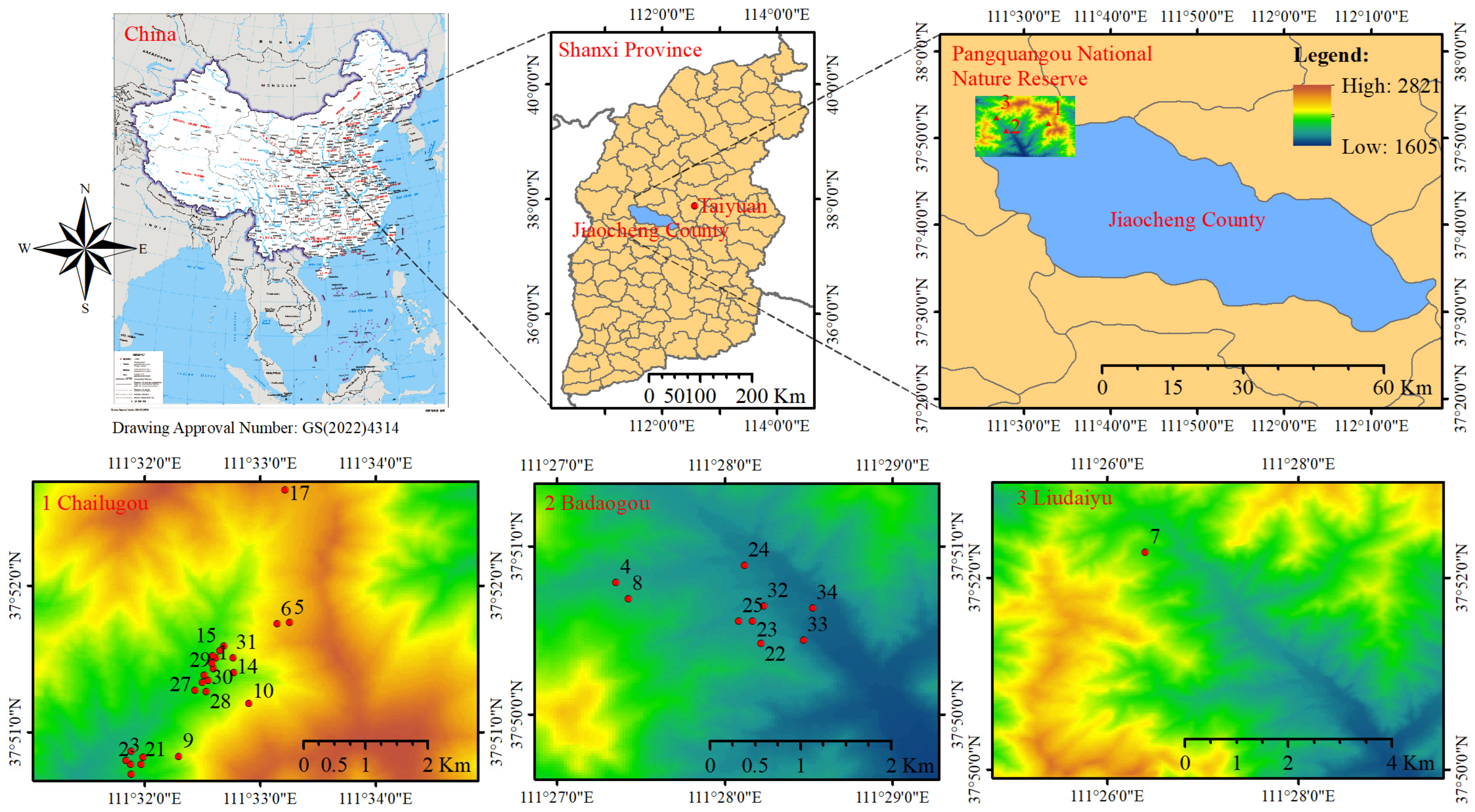
Figure 1. Study area and sample plots. Note: Red dots represent sample plots.
Forests 16 01778 g001
Figure 2. The architecture of the DNN used in this study.
Forests 16 01778 g002
Figure 3. The MSE and MAE values of various models on the training and validation datasets 1 vary with increasing epochs. Each subfigure depicts the training and validation MSE or MAE over epochs.
Forests 16 01778 g003aForests 16 01778 g003b
Figure 4. The MSE and MAE values of various models on the training and validation datasets 2 vary with increasing epochs. Each subfigure depicts the training and validation MSE or MAE over epochs.
Forests 16 01778 g004aForests 16 01778 g004b
Figure 5. Relationship between predicted and observed CW for various models on the test datasets 1. Each subfigure compares the predicted and observed values.
Forests 16 01778 g005
Figure 6. Relationship between predicted and observed CW for various models on the test datasets 2. Each subfigure compares the predicted and observed values.
Forests 16 01778 g006
Figure 7. The residual distribution plots of various models on the test datasets 1. Each subfigure presents the residual distribution for a corresponding model.
Forests 16 01778 g007
Figure 8. The residual distribution plots of various models on the test datasets 2. Each subfigure presents the residual distribution for a corresponding model.
Forests 16 01778 g008
Figure 9. The top 15 important feature plots of various models on the test datasets 1. Each subfigure presents a bar plot of the correlation coefficients between the top 15 selected variables and CW.
Forests 16 01778 g009
Figure 10. The top 15 important feature plots of various models on the test datasets 2. Each subfigure presents a bar plot of the correlation coefficients between the top 15 selected variables and CW.
Forests 16 01778 g010aForests 16 01778 g010b
Table 1. Statistical metrics table for sample trees (n = 1884) and plots (n = 34).
Statistical MetricsCW
/m
DBH
/cm
H
/m
HD
/m
Stem per Hectare /NDg
/cm
Arithmetic Average H/m
Min.1.55.05.119.310815.79.7
Max.14.470.339.839.21,00039.629.8
Ave. ± SD5.0 ± 1.926.7 ± 12.420.3 ± 8.727.5 ± 4.2475.6 ± 189.927.1 ± 4.518.6 ± 4.4
Table 2. Hyperparameter values per tier across model architecture complexity variants.
Tier no.Hyperparameter
Hidden_LayersUnitsKernel_InitializerKernel_RegularizerDropOut_RateOptimizerLearning_RateActivationBatch_Size
1[2,3,4,5][1, 2, 4, 8, 16, 32, 64, 128, 256][‘he_normal’][‘l2(0.0001)’][0.2][‘adam’][1e−4][‘relu’][32, 64, 96, 128, 256]
2[2,3,4,5][16, 32, 64, 128] (Data-scaled)[‘he_normal’][‘l2(0.0001)’][0.2][‘adam’][1e−4][‘relu’][32, 64, 96, 128, 256]
3[2,3,4,5][16, 32, 64, 128] (Data-scaled)[‘he_normal’]‘l2_reg’, min_value = 1e−6, max_value = 1e−3, sampling = ‘log’‘min’: 0.1, ‘max’: 0.4, ‘sampling’: ‘linear’[‘adam’][1e−4][‘relu’][32, 64, 96, 128, 256]
4[2,3,4,5][16, 32, 64, 128] (Data-scaled)[‘he_normal’, ‘glorot_uniform’]‘l2_reg’, min_value = 1e−6, max_value = 1e−3, sampling = ‘log’‘min’: 0.1, ‘max’: 0.4, ‘sampling’: ‘linear’[‘adam’, ‘sgd’, ‘rmsprop’]‘min’: 1e−4, ‘max’: 1e−2, ‘sampling’: ‘log’[‘relu’, ‘elu’, ‘selu’]
‘beta_1’: ‘min’: 0.8, ‘max’: 0.999, ‘sampling’: ‘log’
‘beta_2’: ‘min’: 0.9, ‘max’: 0.9999, ‘sampling’: ‘log’
‘epsilon’: ‘min’: 1e−9, ‘max’: 1e−6, ‘sampling’: ‘log’
‘momentum’: ‘min’: 0.8, ‘max’: 0.99, ‘sampling’: ‘log’
‘nesterov’: [True, False]
‘rho’: ‘min’: 0.8, ‘max’: 0.99, ‘sampling’: ‘log’
[32, 64, 96, 128, 256]
Note: ‘log’ indicates that parameter values are sampled on a logarithmic scale, which is appropriate for searching across multiple orders of magnitude.
Table 3. Various models with different combinations of input variables (Non-HTM vs. HTM).
Model No.Comment VariablesDifferent Variables
DNN1-1DBH, Species, H, N, SDI, BA, Dg, Utree, Ctree, Wtree, Mtree, Mstand, Dmax, H ¯ , HDUstand, Cstand, GC, 1-D, H′, Wstand, R, CVd, K
DNN2-1
DNN3-1
DNN4-1
DNN1-2DBH, Species, H, N, SDI, BA, Dg, Utree, Ctree, Wtree, Mtree, Mstand, Dmax, H ¯ , HDUstand 15, Cstand 15, GC15, 1-D 15, H15, Wstand 15, R15, CVd15, K15
DNN2-2
DNN3-2
DNN4-2
Note: the subscript 15 indicates that the tree height threshold is set to 15 m.
Table 4. The fitting statistics and 10-fold cross-validation results of 8 regression models (mean ± SD).
Model No.Validating Folds Fitting StatisticsTraining Fold Fitting Statistics
R2MSEMAE/mMAPE/%MSEMAE/mMAPE/%
DNN1-10.68 ± 0.050.31 ± 0.020.42 ± 0.02715.33 ± 965.410.30 ± 0.020.42 ± 0.01558.09 ± 526.73
DNN2-10.66 ± 0.040.33 ± 0.040.44 ± 0.03857.97 ± 1241.280.36 ± 0.020.46 ± 0.01649.48 ± 717.86
DNN3-10.68 ± 0.050.30 ± 0.020.42 ± 0.02917.86 ± 1424.770.27 ± 0.030.40 ± 0.02560.50 ± 576.08
DNN4-10.69 ± 0.040.30 ± 0.020.41 ± 0.02903.65 ± 1346.820.30 ± 0.020.42 ± 0.02513.28 ± 443.82
DNN1-2 0.68 ± 0.050.31 ± 0.020.43 ± 0.02776.21 ± 1110.310.32 ± 0.020.44 ± 0.01829.25 ± 743.02
DNN2-20.67 ± 0.040.31 ± 0.010.43 ± 0.02618.97 ± 777.870.30 ± 0.030.42 ± 0.02783.12 ± 719.93
DNN3-20.70 ± 0.050.29 ± 0.020.41 ± 0.01764.40 ± 1053.720.25 ± 0.020.38 ± 0.1733.68 ± 634.74
DNN4-20.71 ± 0.040.29 ± 0.020.41 ± 0.02653.75 ± 785.170.25 ± 0.030.38 ± 0.02614.02 ± 601.40
Disclaimer/Publisher’s Note: The statements, opinions and data contained in all publications are solely those of the individual author(s) and contributor(s) and not of MDPI and/or the editor(s). MDPI and/or the editor(s) disclaim responsibility for any injury to people or property resulting from any ideas, methods, instructions or products referred to in the content.