Article

Forest Aboveground Biomass Estimation Using High-Resolution Imagery and Integrated Machine Learning

1
School of Transportation and Geomatics Engineering, Shenyang Jianzhu University, Shenyang 110168, China
2
Chinese Academy of Surveying and Mapping, Beijing 100830, China
3
Precision Forestry Key Laboratory of Beijing, Beijing Forestry University, Beijing 100083, China
4
Beijing Gardening and Greening Planning and Resource Monitoring Center (Beijing Forestry Carbon Sink and International Cooperation Center), Beijing 101118, China
*
Author to whom correspondence should be addressed.
Forests 2025, 16(12), 1777; https://doi.org/10.3390/f16121777
Submission received: 12 October 2025 / Revised: 10 November 2025 / Accepted: 15 November 2025 / Published: 26 November 2025
(This article belongs to the Section Forest Inventory, Modeling and Remote Sensing)

Abstract

This study quantifies forest aboveground biomass (AGB) using integrated remote sensing features from high-resolution GaoFen-7 (GF-7) satellite imagery. We combined texture features, vegetation indices, and RGB spectral bands to improve estimation accuracy. Three machine learning algorithms—Random Forest (RF), Gradient Boosting Tree (GBT), and XGBoost—were compared with a stacking ensemble model using five-fold cross-validation on forest plots in Beijing’s Daxing District. Feature importance was evaluated through SHAP to identify key predictive variables. Results show that texture features exhibit scale-dependent predictive power, while visible-band vegetation indices strongly correlate with AGB. The Stacking ensemble achieved optimal performance (R2 = 0.62, RMSE = 57.34 Mg/ha, MAE = 39.99 Mg/ha), outperforming XGBoost (R2 = 0.59), RF (R2 = 0.58), and GBT (R2 = 0.57). Compared to the best individual model, Stacking improved R2 by 5.1% and effectively mitigated over- and underestimation biases. These findings demonstrate the effectiveness of ensemble learning for forest AGB estimation and suggest potential for regional-scale carbon monitoring applications.

1. Introduction

Forest aboveground biomass (AGB) quantifies carbon storage in forest ecosystems. It informs climate mitigation strategies, carbon inventories [1], and ecosystem service valuation [2,3]. However, accurate regional-scale estimates remain challenging and critical for effective carbon management policies.
While conventional field-based inventories deliver accurate biomass measurements, they are labor-intensive, costly, and impractical for large-scale, repeated monitoring. The emergence and rapid evolution of satellite remote sensing technologies have positioned space-based forest AGB assessment methodologies at the forefront of research attention. Early studies used moderate-resolution imagery (Landsat, MODIS) [4], later advancing to fine-scale optical data and multi-sensor approaches [5,6]. Feature extraction methodologies have evolved from single spectral band utilization to comprehensive multi-dimensional parameter integration incorporating spectral, textural, and vegetation index components. Dupuy et al. [7] showed that textural attributes capture canopy structural variability, while Sa and Fan [8] confirmed the effectiveness of multi-scale texture analysis. Vegetation indices, representing key biophysical indicators of plant vitality, contribute significantly to forest AGB assessment, with normalized difference vegetation index (NDVI) and enhanced vegetation index (EVI) proving particularly effective in quantifying canopy leaf density and physiological characteristics [9].
Conventional linear and polynomial regression methods have yielded to machine learning. Non-parametric approaches including random forest (RF) [10], support vector machines (SVMs) [11], and gradient boosting methods such as gradient boosting tree (GBT) [12] and Extreme Gradient Boosting (XGBoost) [13] have demonstrated substantial advantages in processing multi-dimensional remote sensing datasets and capturing complex forest structural patterns [14]. Contemporary research has increasingly recognized ensemble learning strategies as pivotal techniques for advancing model prediction capabilities. Wu et al. [15] used multi-model averaging to improve biomass prediction. Tian et al. [16] developed stacking ensemble models with excellent generalization under complex topography. Zhang et al. [17] found that stacking effectively integrates advantages of base learners. Recent work has explored optimized gradient boosting and deep learning. Huang et al. [18] used Categorical Boosting (CatBoost) with hyperparameter tuning on multi-temporal Landsat data to estimate subtropical forest carbon storage. Zheng et al. [19] showed that Light Gradient Boosting Machine (LightGBM) effectively captured regional forest carbon patterns, outperforming other tree-based models. Hiebl et al. [20] employed Sentinel-2 time series with a Convolutional Neural Network (CNN) to map evergreen broad-leaved cover, achieving improved spatial generalization.
Nevertheless, several critical gaps persist in existing forest AGB estimation research. This study directly addresses them using sub-meter (0.65 m) GaoFen-7 (GF-7) RGB imagery and field inventory data from Daxing District, Beijing. We quantify the contribution of RGB spectral bands, visible-spectrum vegetation indices, and fine-scale texture features (3 × 3 pixel, ~2 m), clarifying how high-resolution RGB improves AGB estimation—a gap in prior GF-series and Sentinel studies. We compare four algorithms (RF, GBT, XGBoost, and stacking ensemble) using identical plots and features, isolating algorithmic performance without confounding factors. This study tests the hypotheses that fine-scale texture features from sub-meter RGB imagery provide substantial predictive power for AGB estimation, that vegetation indices from visible bands maintain robust relationships with AGB without near-infrared information, and that stacking ensembles surpass individual base learners in accuracy and bias reduction. Using five-fold cross-validation, we quantify how different feature types contribute to AGB prediction, evaluate algorithm performance, and assess stacking ensemble effectiveness, demonstrating an RGB-only workflow for district-scale AGB mapping.
This approach addresses a practical need for regional carbon management. Beijing aims to increase forest carbon sinks by 1.5 million tons CO2 annually by 2035 to support carbon neutrality goals. Cost-effective RGB-based monitoring enables landscape-scale forest assessment without expensive multispectral sensors, making it accessible for resource-limited regional agencies. If RGB imagery proves sufficient for AGB estimation, this method could be scaled across Beijing’s 16 districts and applied to similar peri-urban forests globally, supporting carbon inventory reporting and forest management decisions.

2. Materials and Methods

The methodology followed a compact, end-to-end framework for quantifying forest AGB from satellite observations and computational modeling (Figure 1). Ground surveys provided reference AGB for model calibration and validation. High-resolution GF-7 imagery (0.65 m) was preprocessed using ENVI (Version 5.6, Broomfield, CO, USA), including radiometric, atmospheric, and geometric corrections. Predictors including spectral bands, vegetation indices, and multi-scale texture features were then derived using ENVI and ArcGIS (Version 10.8, Redlands, CA, USA). RF, GBT, XGBoost, and a Stacking ensemble were developed and evaluated in Python (Version 3.10, Wilmington, DE, USA) using scikit-learn and XGBoost with 5-fold cross-validation. Performance was assessed by the coefficient of determination R-squared (R2), root mean squared error (RMSE) and mean absolute error (MAE). The Shapley Additive Explanations method (SHAP) [21] was used to identify key variables and improve interpretability. The optimal model produced wall-to-wall AGB maps across Daxing District, with residual analysis for accuracy diagnostics.

2.1. Study Area

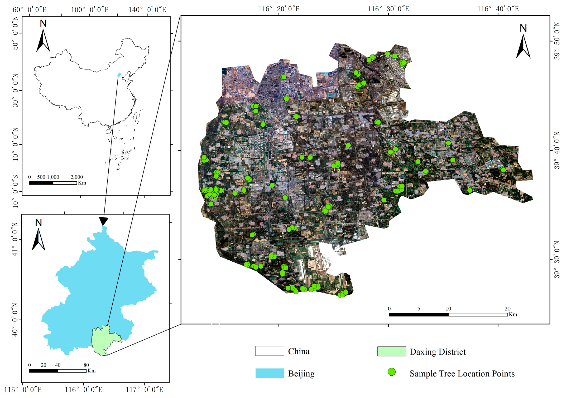
This study focuses on Daxing District, Beijing (39°26′–39°51′ N, 116°13′–116°43′ E, WGS-84), covering approximately 1036 km2 (Figure 2). Located in southern Beijing, the district represents a typical plain region transitioning from the North China Plain toward the Yanshan Mountains. The district has flat terrain (elevations 15–60 m) with gentle northwest-to-southeast slopes. Slopes are predominantly below 3°, making this area representative of typical plain forest ecosystems.
The region has a warm temperate semi-humid continental monsoon climate with mean annual temperature of 11.6 °C and precipitation of ~550 mm, concentrated in June-August. The region is situated on the Yongding River alluvial fan and the ancient Yellow River alluvial plain, with soils dominated by fluvo-aquic and cinnamon soil types. The deep soil layers provide favorable site conditions for forest vegetation growth. Forest vegetation consists predominantly of plantation forests and farmland shelterbelts established through afforestation programs, though many stands have since undergone natural succession.
The dominant forest types include poplar (Populus spp.) plantations, black locust (Robinia pseudoacacia) shelter forests, Japanese pagoda tree (Styphnolobium japonicum) landscape forests, and small populations of coniferous species including Chinese pine (P. tabulaeformis) alongside oriental arborvitae (P. orientalis). Forests occur primarily along roadsides, field boundaries, riparian zones, and urban green belts in linear and patchy patterns. Stand structure is relatively simple, consisting mainly of monocultures or simple mixed stands. The forests are predominantly young to middle-aged, with average diameter at breast height (DBH) of 15–25 cm and stand density of 400–1200 stems ha−1. While established as plantations during 1990–2010, these stands have undergone 15–30 years of natural succession with minimal silvicultural intervention, functioning primarily as shelterbelts under semi-natural management. This extensive management has allowed natural processes to occur, with growth patterns resembling naturally regenerated forests of comparable age, supporting the use of regional allometric equations (Equations (1) and (2)).
Daxing District maintains approximately 25% forest coverage, which, while lower than mountainous regions, represents a crucial ecological functional zone within Beijing’s plain areas. The forests serve vital roles in windbreak and sand stabilization, soil and water conservation, air purification, and carbon sequestration. Daxing District represents typical semi-naturally managed plantations across the North China Plain, enabling validation of high-resolution remote sensing for AGB estimation and providing methodological guidance for regional carbon inventories and ecosystem service assessments.

2.2. Data Collection and Preprocessing

2.2.1. Field Survey Data

Field surveys were conducted in Daxing District, Beijing, from May to September 2024, establishing an AGB database from 1344 sample plots (Table 1). Plot establishment followed national forestry inventory protocols to ensure standardized data collection. Within each plot, all trees with DBH ≥ 5 cm were measured at 1.3 m above ground using diameter tapes with 0.1 cm precision and tree height was measured with laser rangefinders. Additional dendrometric parameters, together with stand attributes such as forest type, stand age, slope, and aspect, were recorded systematically. Real-Time Kinematic—Global Navigation Satellite System (RTK-GNSS) was used to determine plot coordinates with <1 m positional accuracy to meet image–ground registration requirements.
Sample plots were distributed evenly across the study area, spanning diverse forest types, elevations, and slope aspects to minimize bias and maximize tree species diversity and forest type representation. Tree-level biomass estimation employed the generalized allometric equation from Tang et al. [22] for major tree species in Chinese forests as follows:
A G B i = 0.048 × D B H 1.9276 × H 0.9638
where A G B i is the above-ground biomass of tree i   (kg), D B H is the diameter at breast height (cm) and H is tree height (m).
A nested plot design stratified by DBH size classes was employed to accommodate the density distribution patterns observed in preliminary surveys. Subplot areas were set at 4 m2 (DBH 5–12 cm), 9 m2 (DBH 12–20 cm), 12.25 m2 (DBH 20–30 cm), and 20.25 m2 (DBH > 30 cm) to ensure adequate sampling of larger trees while maintaining field efficiency for smaller, more abundant stems. Plot-scale AGB was calculated as:
A G B S = j = 1 4 i = 1 n j A G B i j A j × 10
where A G B i j represents individual tree biomass for the i-th tree in DBH class j (kg), n j is the number of trees in DBH class j, and A j is the corresponding subplot area (m2). The factor ×10 converts kg/m2 to Mg/ha (10,000 m2/ha÷1000 kg/Mg = 10).

2.2.2. Remote Sensing Data

This study utilized GF-7 satellite data as the primary remote sensing data source [23]. GF-7 is China’s first sub-meter stereoscopic mapping satellite with 0.65 m panchromatic and 2.6 m multispectral sensors and a 5-day revisit period, providing high-quality forest coverage. The delivered dataset contained RGB bands at 0.65 m resolution (Blue 0.45–0.52 μm, Green 0.52–0.59 μm, Red 0.63–0.69 μm). The NIR band (~0.77–0.89 μm) was unavailable, precluding NIR-based indices (NDVI, EVI, SAVI); therefore, we focused on visible-band indices and Gray-Level Co-occurrence Matrix (GLCM) texture features.
Imagery data were acquired primarily from 11 May 2024, and 11 September 2024, temporally synchronized with field survey periods to ensure high consistency between remote sensing and ground measurements. Due to suboptimal image quality in some areas during June–September 2024, supplementary images from adjacent years (23 May 2023, and 26 August 2025) were incorporated. The 2024 imagery provided 87.25% coverage of the Daxing District study area, with temporal gaps filled by phenologically matched scenes from near-anniversary dates. The GF-7 satellite imagery was obtained from the China Centre for Resources Satellite Data and Application (https://sasclouds.com/chinese/home/, accessed on 15 October 2024). Images with <25% cloud coverage were selected, yielding 8 GF-7 scenes covering the study area. This temporal matching minimizes phenological variations and ensures data reliability for AGB estimation.
Satellite imagery preprocessing was performed in ENVI 5.6 following established protocols. Raw digital numbers were radiometrically calibrated to at-sensor radiance using sensor-specific coefficients stored in the image metadata. Surface reflectance was retrieved using the Fast Line-of-sight Atmospheric Analysis of Spectral Hypercubes (FLAASH) module [24], which employs radiative transfer modeling to compensate for atmospheric effects. Geometric rectification used 134 ground control points from a high-resolution JiLin-1 (JL-1) orthoimage, yielding RMSE < 1 pixel (0.5 m). Multi-temporal image registration ensured sub-pixel alignment among acquisition dates. Mosaicking applied histogram matching and feathering in overlap zones, with visual and statistical checks confirming no radiometric discontinuities. The final product provided seamless, geometrically and radiometrically consistent imagery.

2.3. Feature Extraction and Selection

Textural characteristics were derived using the GLCM [25]. GLCM quantifies second-order spatial dependence in pixel intensities and is effective for characterizing canopy structure. Based on recent studies showing that smaller windows (≈3 × 3–5 × 5) preserve fine-scale canopy texture and often outperform larger windows for biomass/structure estimation [14,26,27], and to match the plot-scale footprint, this study employed a 3 × 3 pixel window scale for texture feature extraction. Using the GLCM algorithm with a direction angle of θ = 45° and displacement distance of d = 1, eight texture features were extracted (Table 2):
The selection of vegetation indices for this research was confined to those derived from visible light bands. Based on a comprehensive literature review [28,29,30] and preliminary experiments, four visible-band indices demonstrating sensitivity to forest biomass were identified, the definitions of these indexes are provided in Table 3:

2.4. Machine Learning Modeling

Given the high spatial resolution of satellite imagery, sample plots served as the basic sampling unit, with remote sensing features extracted from 3 × 3 pixel windows centered on each plot location, yielding 1344 independent samples with corresponding field-measured plot-level AGB and tree parameters (height and DBH). Five-fold cross-validation was employed for model training and evaluation, where the dataset was randomly partitioned into five equal subsets, with each iteration using four subsets (80%) for training and one subset (20%) for testing, and final model performance evaluated based on aggregated statistics across all five folds, with uncertainty quantified using 95% confidence intervals for key metrics (R2 and RMSE). Three machine learning algorithms, including RF, GBT and XGBoost were applied as base learners, followed by ensemble learning strategies to improve prediction accuracy.

2.4.1. Random Forest

The RF algorithm enhances predictive capability and robustness through ensemble learning with multiple decision trees [10]. This algorithm employs bootstrap sampling and random feature selection to effectively mitigate overfitting risks. To optimize model performance, we conducted hyperparameter tuning for three critical parameters: the number of trees (ntree), maximum tree depth (maxdepth), and the number of features randomly sampled at each split (mtry). A grid search strategy was implemented with ntree ranging from 100 to 1000 (increments of 100), maxdepth ranging from 5 to 15, and mtry ranging from 2 to 10. The optimization process utilized five-fold cross-validation to minimize RMSE and prevent overfitting. Through this systematic search, the optimal parameter configuration was identified as ntree = 500, maxdepth = 10, and mtry = 5. Model construction was conducted using the RF package in R software (version 4.3.1; R Core Team, Vienna, Austria) [35]. The mathematical formulation is expressed as follows:
h R F x = 1 B b = 1 B T b x
where B is the number of trees and Tb(x) is the prediction of the b-th tree.

2.4.2. Gradient Boosting Tree

GBT utilizes a sequential ensemble approach that iteratively minimizes prediction errors through successive decision tree construction [12]. Subsequent trees are trained on the residual errors from previous iterations, leveraging gradient-based optimization techniques to reduce the objective function. Model efficacy is determined by key tuning parameters: step size (learning rate), ensemble size (tree count), and structural complexity (maximum tree depth). The step size regulates the balance between convergence efficiency and generalization capability, whereas ensemble size and structural complexity dictate the model’s representational power and predictive capacity. Through systematic hyperparameter tuning, the optimal configuration was determined with a step size of 0.05, an ensemble of 200 trees, and structural depth of 6, achieving superior validation metrics.
At iteration t = 1, …, T, the model is updated as
h G B T ( x ) = F t x = F t 1 x + ν h t x
where x is the input vector, F t 1 x and F x are the predictions at iterations t − 1 and t, ν 0,1 is the learning rate (step size), h t ( x ) is the regression tree fitted at iteration t, t is the iteration index, and T is the total number of boosting iterations.

2.4.3. Extreme Gradient Boosting

XGBoost provides an enhanced implementation of gradient boosting by exploiting first- and second-order derivatives of the objective during tree building [13], which enables faster convergence and improved predictive performance. The framework includes built-in regularization to mitigate overfitting and supports column/row subsampling for additional stochasticity and computational efficiency. Key tuning parameters include the step size (learning rate), number of trees, maximum tree depth, and the feature/instance subsampling rates. Following comprehensive hyper-parameter optimization, the best-performing configuration was step size = 0.05, 200 estimators, maximum depth = 6, feature subsampling = 0.8, and instance subsampling = 0.8, yielding the best cross-validation results.
After T boosting rounds, the additive model is
h X G B o o s t = y ^ T x = t = 1 T η · f t x
where T is the number of boosting rounds, η is the learning rate, and f t x is the prediction of the t -th regression tree for input x. Each f t is learned by minimizing the regularized objective.

2.4.4. Stacking Ensemble Learning

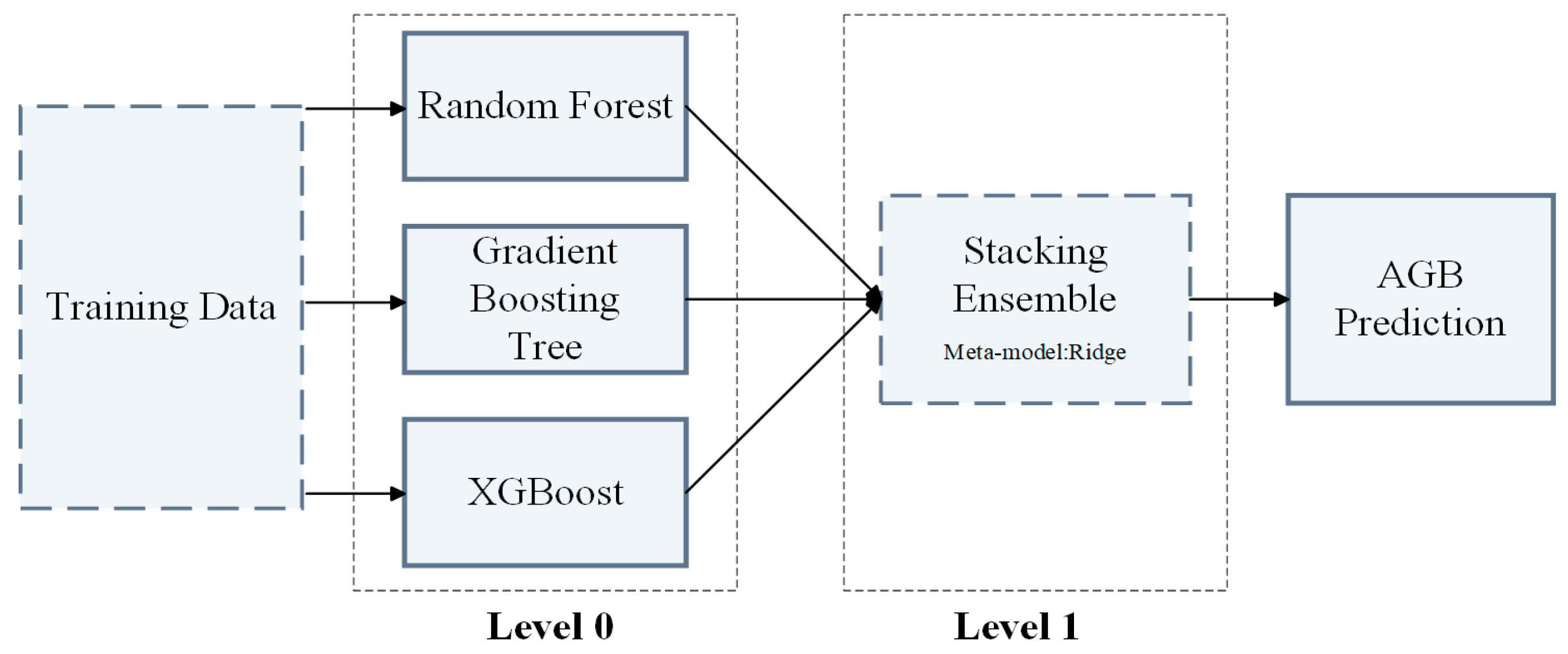
Stacking ensemble learning represents an advanced ensemble strategy implemented after the completion of all base learner training (level 0). The workflow of this strategy is illustrated in Figure 3. Stacking, also known as stacked generalization, effectively integrates the predictive capabilities of different algorithms through meta-learning approaches. The core principle of this method involves utilizing a level 1 meta-learner to derive optimal combination strategies from the predictions generated by base models (level 0). By estimating the generalization bias of base learners and minimizing these biases during the ensemble process, this approach achieves substantial improvements in predictive performance [36,37].
This research employed RF, GBT, and XGBoost as base learners in the Level 0 ensemble architecture. Ridge Regression [38] was selected as the Level 1 meta-learner, with the regularization parameter α and hyperparameters for all base learners optimized through comprehensive grid search with cross-validation. The stacking ensemble model is mathematically expressed as:
H x = w 1 · h R F x + w 2 · h G B T x + w 3 · h X G B o o s t x + b
where h R F ( x ) , h G B T ( x ) and h X G B o o s t ( x ) represent the prediction outputs of the three base learners for input x (in Mg/ha), and w 1 , w 2 , w 3 are the weights assigned to each base learner, and b is the intercept term. All coefficients are estimated by the Ridge Regression meta-learner to optimize predictive performance.

2.5. Model Validation and Evaluation

A five-fold cross-validation approach was implemented for model performance evaluation. The dataset was randomly divided into five equal folds, with each fold serving as the test set once while the remaining four served as training sets. Performance metrics were computed by averaging results across all folds to ensure robust evaluation.
Multiple statistical metrics were used to assess model performance. R2 and RMSE served as primary metrics, with R2 measuring explained variance and RMSE quantifying prediction errors. Furthermore, mean error (ME), mean relative error (MRE), and mean MAE provided comprehensive assessment of model performance, offering different analytical perspectives on prediction precision and consistency.
R 2 = 1 j = 1 N Q j Q ^ j 2 j = 1 N Q j Q ¯ j 2
R M S E = j = 1 N Q ^ j Q j 2 N
M E = j = 1 N Q ^ j Q j N
M R E = 1 N j = 1 N Q j Q ^ j Q j
M A E = 1 N j = 1 N Q j Q ^ j
where Q j represents the observed AGB values, Q ^ j represents the predicted AGB values, Q ¯ j represents the mean AGB value of the samples, and N represents the number of samples. (i.e., plots, N = 1344).

3. Results

3.1. Sample Data Characteristics

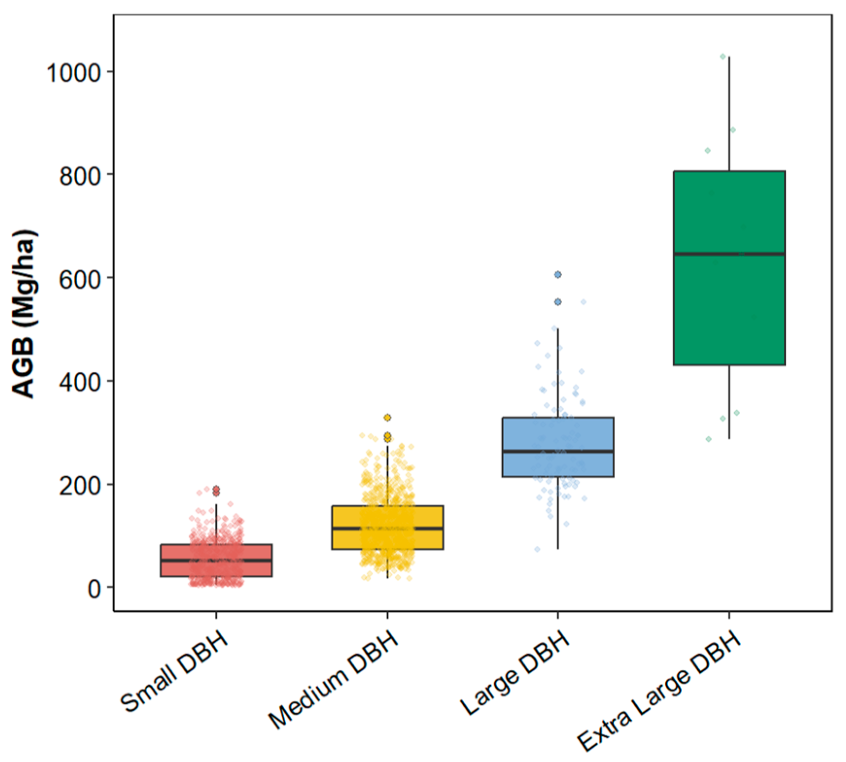
The research examined AGB measurements from 1344 sample plots, where tree DBH ranged from 5.04 to 47.9 cm and plot-level AGB varied from 6.39 to 1028.98 Mg/ha, with an average of 112.95 Mg/ha. Average AGB demonstrated a pronounced upward progression through diameter categories, recording values of 54.366 ± 36.712, 119.639 ± 55.853, 279.182 ± 92.477, and 633.946 ± 245.176 Mg/ha, respectively (Figure 4). Single-factor ANOVA testing indicated statistically significant distinctions across diameter categories, with F = 736.167 and p < 0.001. Subsequent pairwise comparison analyses validated that diameter category comparisons all achieved statistical significance (p < 0.001). The specimen composition featured primarily intermediate-diameter trees, aligning with typical diameter distribution patterns observed in natural forest ecosystems. Variation coefficients spanned 33.1% to 67.5%, illustrating the distribution patterns of AGB within various diameter categories.

3.2. Model Performance Comparison

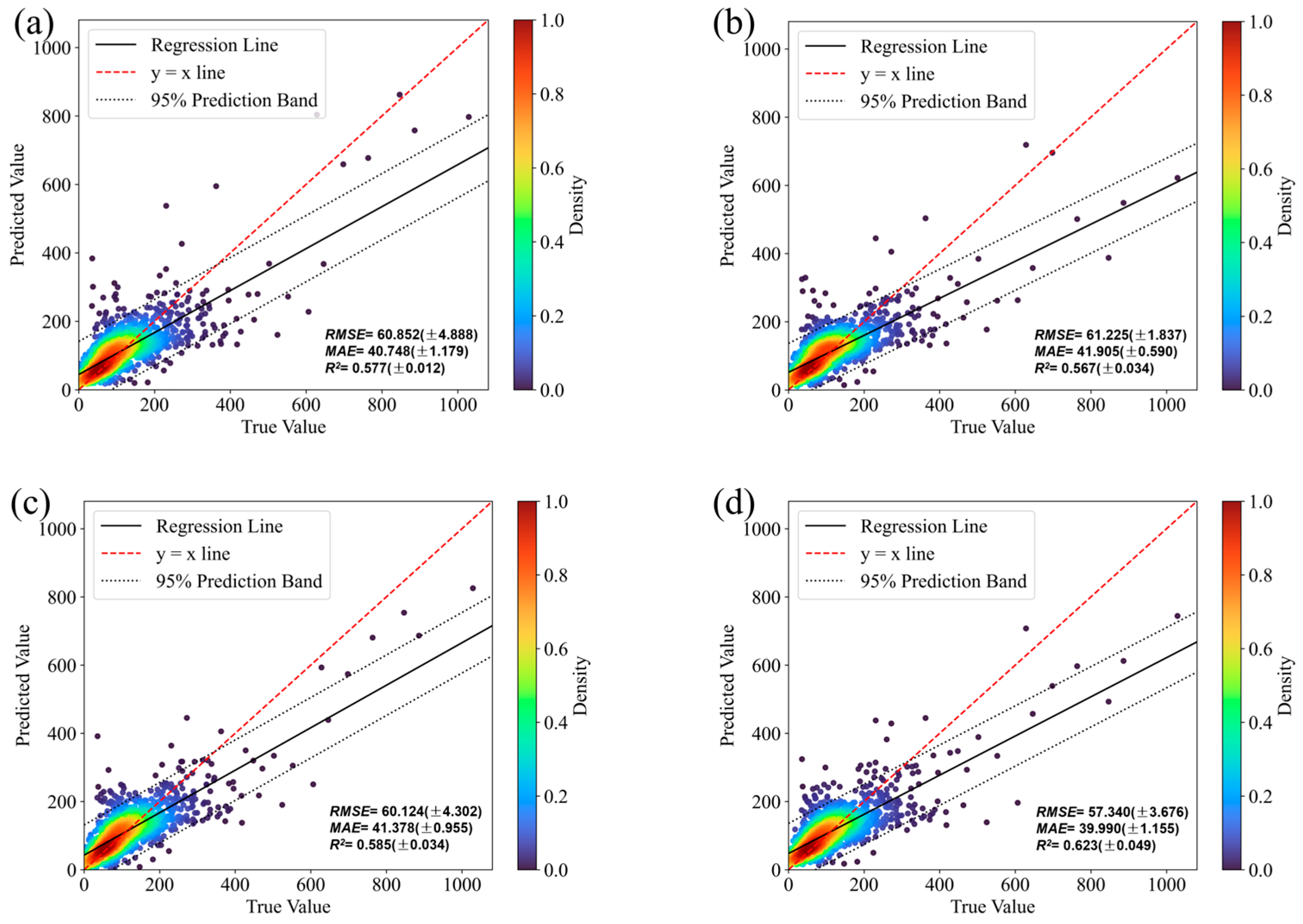
The comparative analysis of four algorithmic approaches for biomass estimation is illustrated in Figure 5. Among the evaluated methods, the ensemble stacking technique yielded the best results with R2 = 0.62 and RMSE = 57.340 Mg/ha. XGBoost ranked second in performance metrics, generating an R2 of 0.59 alongside an RMSE of 60.124 Mg/ha. RF displayed marginally reduced effectiveness compared to XGBoost, producing R2 and RMSE measurements of 0.58 and 60.852 Mg/ha, respectively. The GBT approach yielded the least favorable outcomes, registering an R2 of 0.57 and RMSE of 61.225 Mg/ha.
Quantitative analysis reveals that the stacking method achieved substantial improvements compared to the best-performing individual algorithm, XGBoost, with R2 increasing by 5.1% and RMSE decreasing by 4.6%. Compared to RF, stacking improved R2 by 6.9% and reduced RMSE by 5.8%; compared to GBT, improvements reached 8.77% and 6.4%, respectively.
To investigate the stacking ensemble’s fusion mechanism, we used ridge regression as the meta-learner with the following equation:
H x = 0.354054 h R F x + 0.840168 h G B T x + 0.559010 h X G B o o s t x + 0.000433
The coefficients reflect both the direction and magnitude of each base learner’s contribution to the ensemble. GBT and XGBoost exhibit strong positive weights, indicating their favorable impact on final predictions, while RF’s negative weight compensates for its prediction bias through the meta-learner’s weight adjustment. The near-zero intercept suggests minimal baseline deviation in the model. These results demonstrate that the ridge regression-based Stacking strategy significantly enhances both accuracy and stability in aboveground biomass prediction by optimally combining diverse base models through weighted fusion.

3.3. Model Performance Analysis

Comparison of model performance metrics demonstrated the superiority of the Stacking ensemble over individual base learners (Table 4), achieving the highest explained variance and lowest prediction errors with consistent improvements of 5%–9% in R2 and 4%–6% reductions in error metrics. This enhanced performance stems from the ensemble’s integration of complementary base learner strengths—RF’s non-linear partitioning, GBT’s gradient optimization, and XGBoost’s regularization—through meta-learner optimization of prediction weights. The overlapping 95% confidence intervals indicate modest but statistically consistent gains rather than dramatic superiority, while the narrower error ranges in Stacking reflect improved robustness across validation folds, enhancing confidence for operational district-scale biomass inventory.
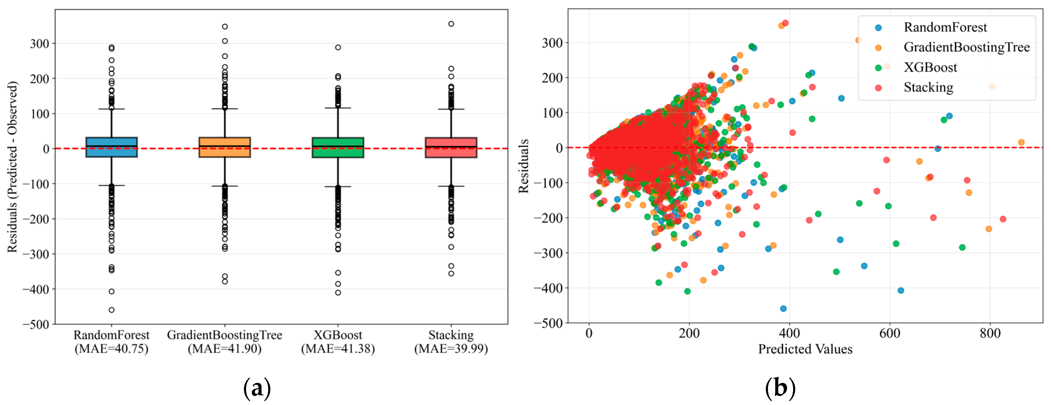
Examination of residual patterns unveiled notable variations in predictive consistency across the four approaches. Shapiro–Wilk normality tests on residuals (n = 1344) showed that although all models significantly deviated from normality (p < 0.001), the Stacking ensemble achieved the highest W statistic (W = 0.93), outperforming RF (W = 0.8832), GBT (W = 0.9158), and XGBoost (W = 0.9122), indicating relatively better approximation to normal distribution. The ensemble stacking method recorded a residual standard deviation of 57.482, substantially below that of RF (60.852), GBT (61.181), and XGBoost (60.124). The Stacking ensemble exhibited skewness of −0.71 and kurtosis of 4.97, representing the most symmetric and least heavy-tailed distribution among all approaches. Boxplot evaluation (Figure 6a) indicated the stacking approach attained an interquartile range of 55.876, with errors extending from −356.084 to 355.657, manifesting optimal symmetric distribution. Conversely, RF demonstrated increased negative anomalies (error lower limit: −459.444), while GBT presented notable positive deviations (upper threshold: 347.904). Investigation of residual-prediction relationships highlighted forecasting consistency disparities (Figure 6b). The stacking methodology produced a residual-prediction correlation of −0.006, nearest to zero across all methods. Mean error values measured −4.779, 1.748, and 2.980 for low, medium, and high prediction intervals, respectively. By contrast, RF, GBT, and XGBoost demonstrated residual-prediction correlations of −0.074, 0.073, and −0.029, with error variability surpassing the stacking approach.
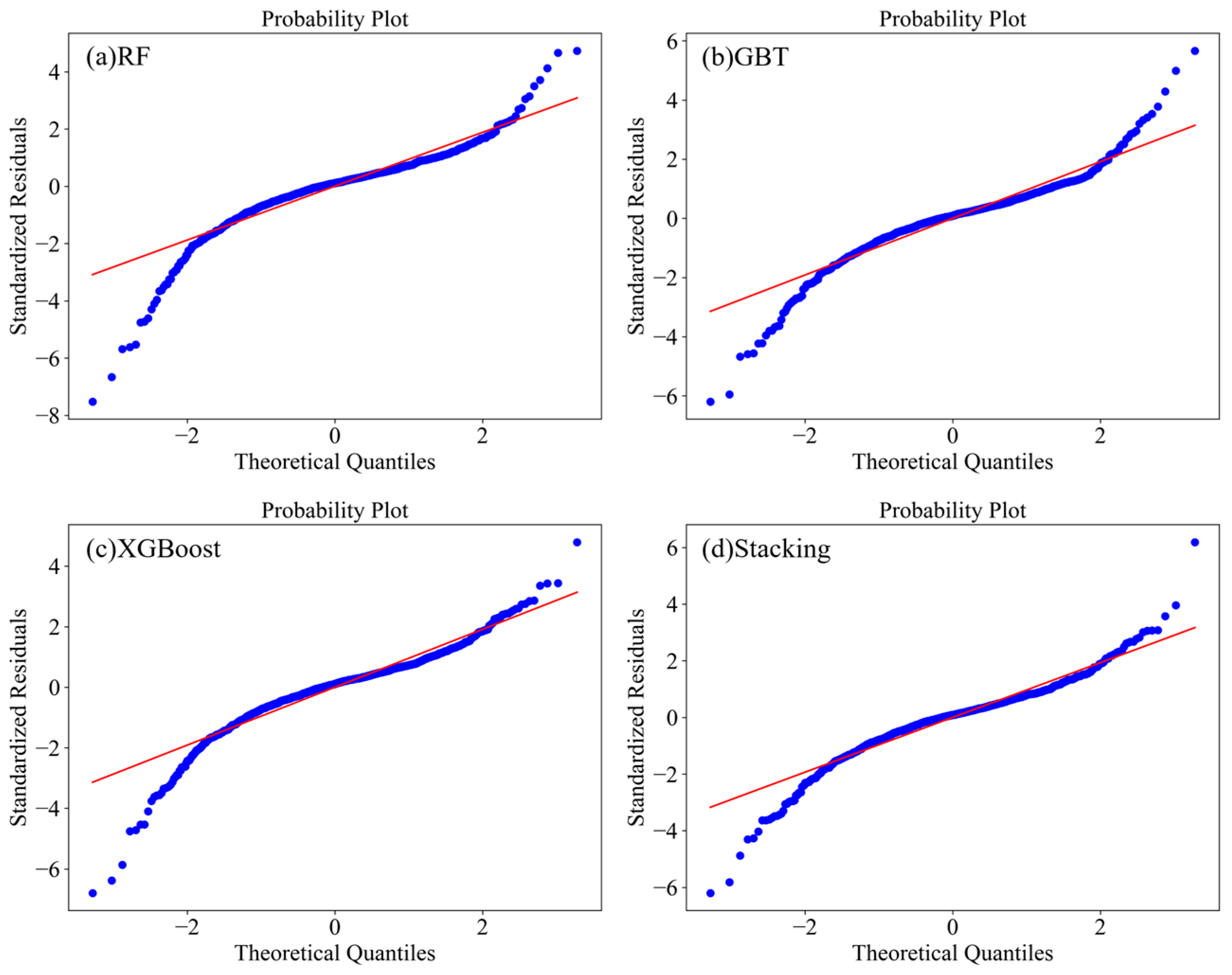
Normality assessments of standardized residuals indicated that the stacking approach demonstrated superior distributional properties (Figure 7). This method attained a Shapiro–Wilk value of 0.93, skewness of −0.71, and kurtosis of 4.97, collectively indicating the nearest conformity to normal distribution across all evaluated approaches. RF produced comparable metrics of 0.88, −1.39, and 8.56, indicating the greatest deviation from normal distribution patterns. The GBT and XGBoost approaches showed Shapiro–Wilk values of 0.92 and 0.91, skewness of −0.72 and −1.161, alongside kurtosis of 5.69 and 6.19, with all metrics falling short of the stacking approach’s standards.

3.4. Feature Importance Analysis

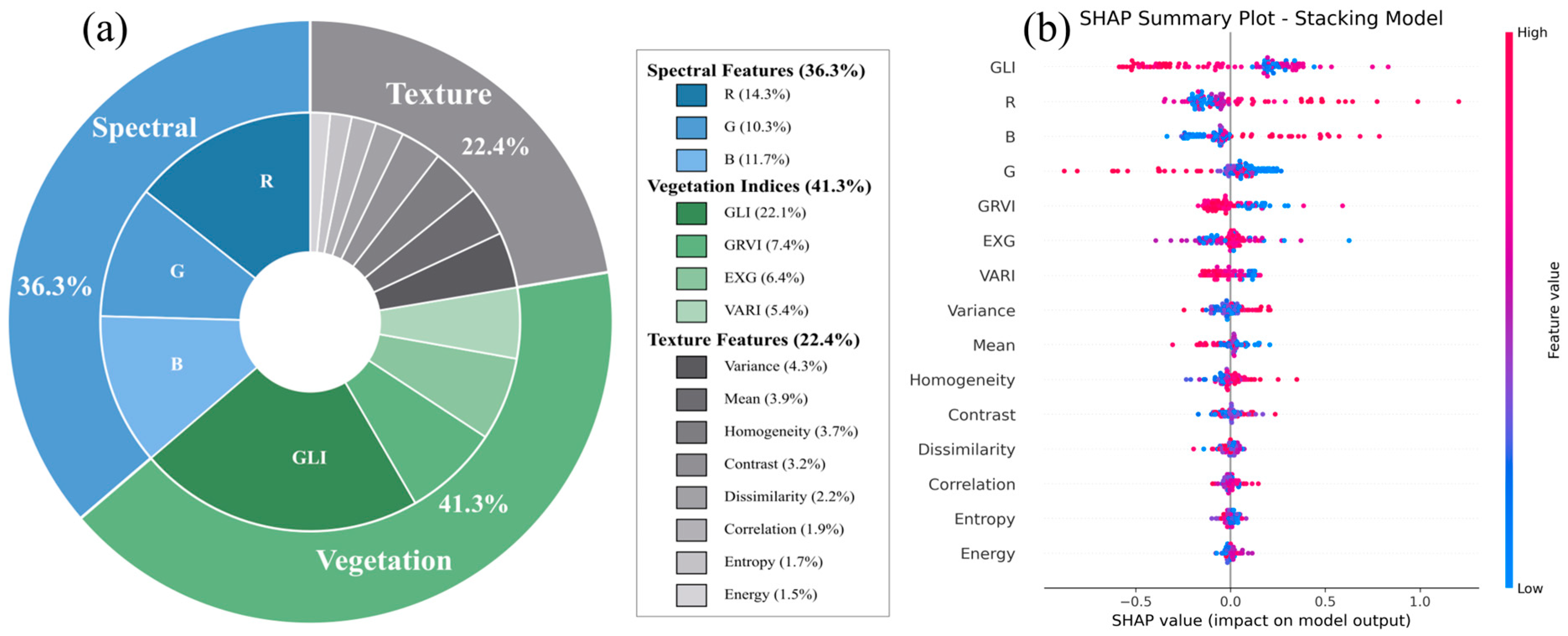
This study evaluated 15 predictors (3 spectral bands, 4 visible-band vegetation indices, and 8 GLCM texture features). Mean absolute SHAP values for the stacking ensemble were normalized to sum to 1.0 across all features (Figure 8a). Vegetation indices contributed the most (41.3%), followed by spectral bands (36.3%) and textures (22.4%). At the feature level, GLI had the largest normalized contribution (22.1%), followed by R (14.3%), B (11.7%), and G (10.3%). The full ranking with both raw and normalized SHAP values is provided in Supplementary Table S1.
The top seven features—all vegetation indices and spectral bands—accounted for 77.6% of total predictive power (Figure 8b). The top four features (GLI, R, B, G) alone contributed 58.3%. The remaining vegetation indices (GRVI, EXG, VARI) ranked 5th–7th with SHAP values of 0.0738, 0.0645, and 0.0546. Within texture features, variance, mean, and homogeneity exhibited the highest importance with SHAP values of 0.0432, 0.0386, and 0.0374, respectively, while contrast, dissimilarity, correlation, entropy, and energy ranged from 0.0153 to 0.0316, all positioned in the lower half of the importance ranking. Although individual texture features showed low importance, their combined contribution reached 22.4%. These SHAP analysis results quantify the relative importance of different feature categories for biomass prediction modeling, providing empirical support for feature selection and model optimization.

4. Discussion

4.1. Benefits of Ensemble Learning in Forest AGB Estimation

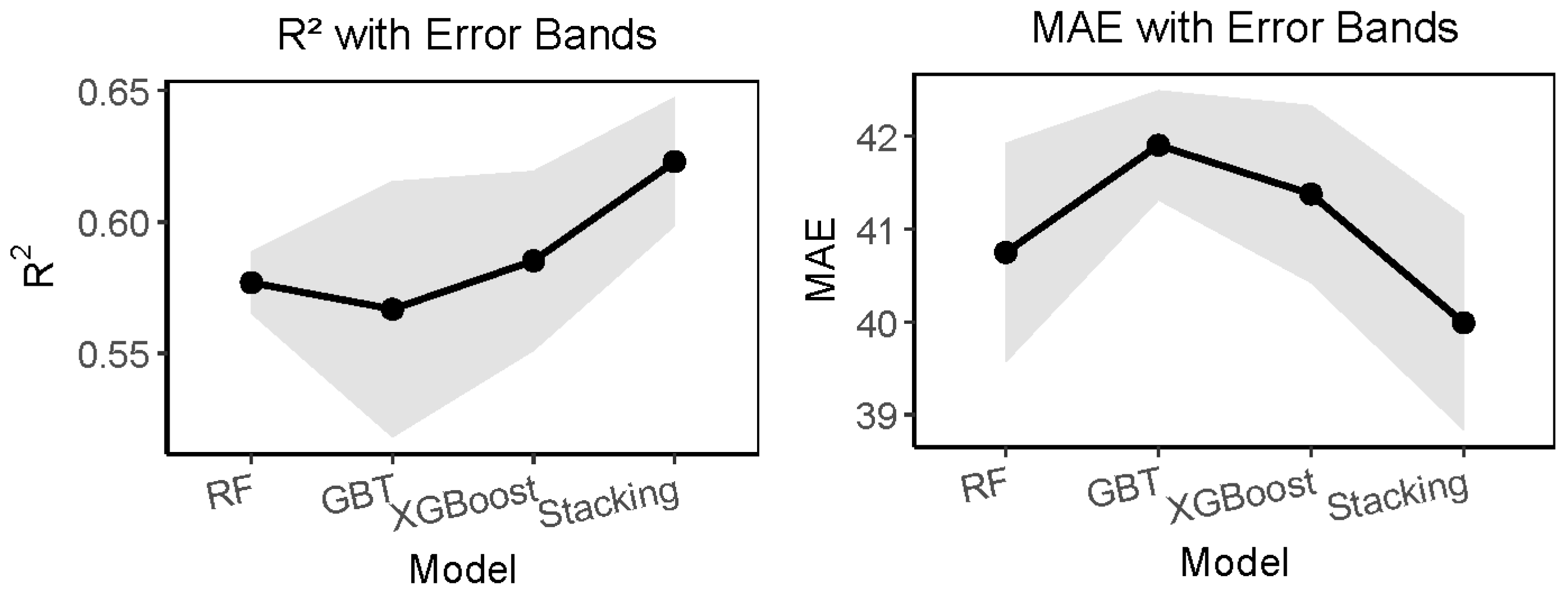
This study estimated forest aboveground biomass in Beijing’s Daxing District using machine learning with GF-7 high-resolution optical imagery. Ensemble learning has gained increasing attention in forest remote-sensing modeling [36,39]. Our Stacking ensemble outperformed individual algorithms in this study area (Figure 9). Our approach demonstrates competitive performance compared with recent methodologies. Tang et al. [22] achieved R2 = 0.65 using RF with Landsat 8 OLI imagery combined with habitat datasets for Pinus forests in Yunnan in 2024, where texture variables played a significant role but required additional environmental data. Zeng et al. [40] reported R2 = 0.64 using RF with polarimetric SAR parameters from C- and L-bands for component biomass estimation, demonstrating the potential of multi-polarization radar data but requiring specialized SAR processing. Wai et al. [41] obtained R2 = 0.52 using RF-based co-Kriging with Sentinel-2 and SRTM data in Myanmar forest reserves, where geostatistical interpolation improved spatial prediction but increased computational complexity. While these approaches achieved competitive accuracies through specialized data sources or processing methods, our Stacking ensemble reached R2 = 0.63 with RMSE of 57.34 Mg/ha using solely GF-7 optical imagery without requiring SAR data, environmental datasets, or geostatistical interpolation. These comparisons demonstrate that ensemble learning with high-resolution optical data offers a practical alternative balancing accuracy with operational simplicity, though differences in study areas, forest types, and field protocols complicate direct comparisons. Compared with traditional single-model approaches, Stacking can identify complementarity among base learners via a meta-learner, avoiding the limitations of simple voting or averaging [39]. This is particularly useful for high-dimensional remote-sensing features, where different algorithms exploit different parts of the feature space [14,42,43]. The meta-learner’s ability to assign optimal weights, including the negative weight for RF that compensates for systematic bias, demonstrates sophistication beyond simple model averaging. When high-quality optical data are available, this ensemble strategy with GF-7 imagery offers practical advantages over workflows requiring specialized data sources or complex processing methods, achieving faster data acquisition at lower cost while maintaining competitive accuracy. In contrast to studies relying on single algorithms [36], our ensemble strategy improved accuracy in this study area and could be extended after broader validation.

4.2. Feature Importance and Underlying Mechanisms

GLI’s exceptional effectiveness aligns with recent advances in visible-band indices. Our GF-7 imagery contained only RGB bands, so analyses were limited to visible indices (EXG, GRVI, VARI, GLI), while NIR-based indices (NDVI, EVI, SAVI) could not be computed, although they are often robust for vegetation characterization [44,45]. GLI performs best by emphasizing green reflectance while de-emphasizing red and blue, which chlorophyll strongly absorbs. As canopy density increases, pixel-level green dominance strengthens, making GLI respond more directly to canopy cover. Its normalization also dampens illumination and shadow variation common at sub-meter scales. In peri-urban settings, typical backgrounds (impervious surfaces, bare soil, rooftops) exhibit weak green dominance and relatively higher red/blue values, so GLI enhances canopy–background contrast [46,47,48] more effectively than other visible indices. Regarding feature collinearity, VIF analysis confirmed notable correlations among vegetation indices. However, our stacking ensemble framework integrating RF, GBT and XGBoost as base learners is inherently robust to multicollinearity through recursive feature partitioning rather than linear coefficients. Leave-one-out validation demonstrated that each index contributes unique variance despite correlations, with stable cross-validation performance showing no overfitting. SHAP importance rankings revealed distinct contribution patterns among correlated predictors, confirming they capture complementary rather than redundant information. Our workflow can incorporate NIR indices when multispectral data becomes available, but the results demonstrate practical value for high-resolution applications relying primarily on visible-band data.
The role of texture features in forest AGB estimation has been a research focus. In this investigation, texture attributes contributed 22.4% to the overall model. Although their standalone significance was comparatively limited, the spatial structural data they deliver remains indispensable [49]. This outcome corresponds with earlier studies that describe texture characteristics as fulfilling a “supportive yet essential” function in forest parameter extraction [26,50]. This is especially apparent in high-resolution imagery, where texture features address spectral limitations in distinguishing forest structural categories. This proves particularly useful in complex urban forest settings [51,52].

4.3. Spatial Distribution Patterns and Application Prospects

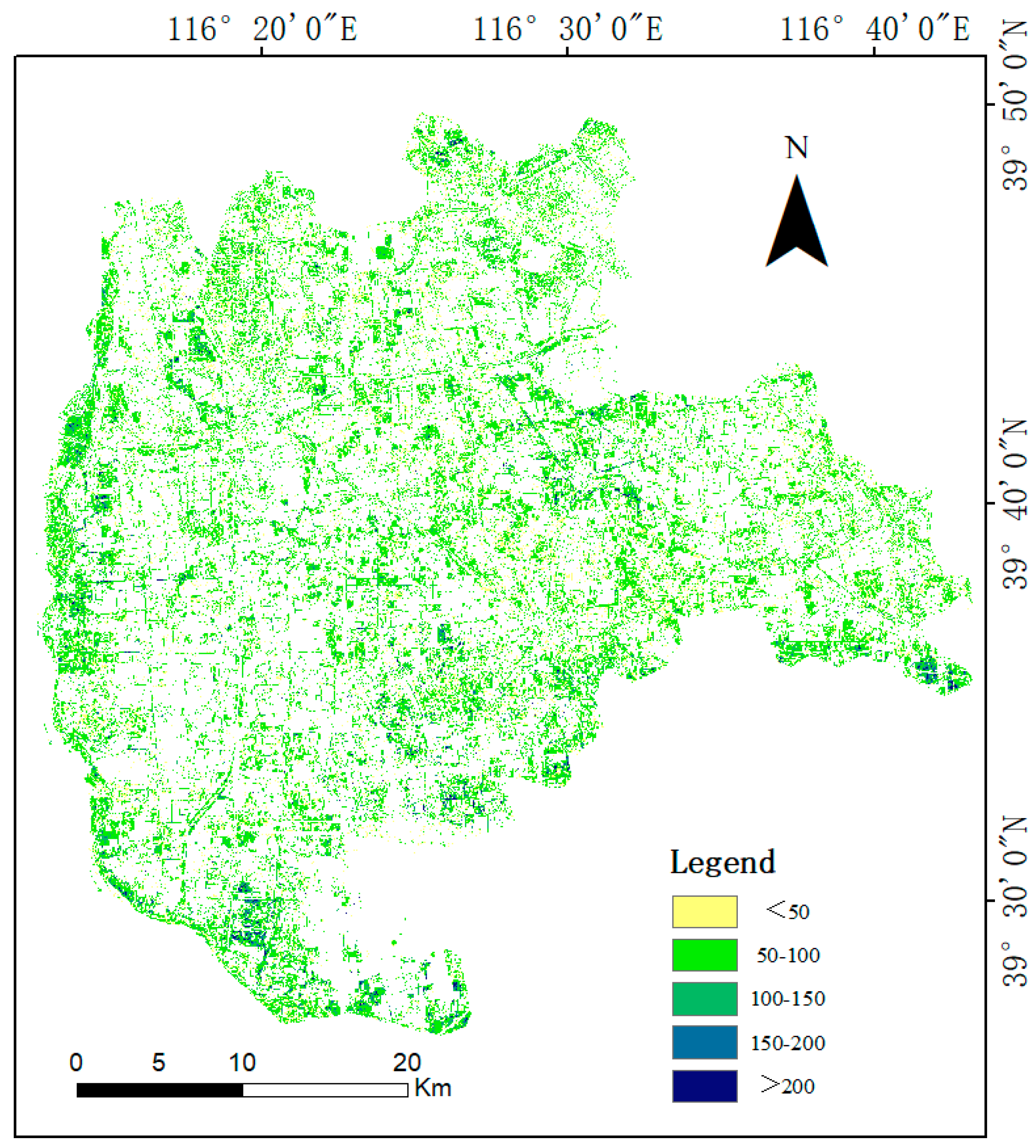
Spatial distribution analysis of forest biomass through the optimized ensemble approach demonstrated significant heterogeneity throughout the investigation region (Figure 10). This investigation developed four different algorithmic approaches—RF, GBT, XGBoost and Stacking—utilizing grid search optimization combined with cross-validation for parameter tuning. Each approach successfully captured the spatial patterns of tree AGB throughout Daxing District, although performance levels varied in terms of accuracy and stability. The ensemble Stacking approach excelled beyond individual methods across evaluation criteria by integrating outputs from multiple base algorithms, resulting in superior predictive consistency. Therefore, the ensemble method was chosen to produce the comprehensive AGB spatial distribution for Daxing District.
The spatial patterns observed here have potential implications for regional carbon monitoring. The achieved model accuracy suggests that district-scale carbon stock estimation could be conducted with reasonable precision for policy planning purposes. For Daxing District’s forest area, this may contribute to carbon inventory data that inform Beijing’s carbon sequestration goals and forest management strategies. These spatial patterns underscore the intricate nature of Beijing’s forest systems and contribute novel perspectives on carbon sequestration patterns within peri-urban forest landscapes [53]. In contrast to earlier research predominantly examining uniform forest stands or single ecosystem types [54,55], this multi-area assessment delivers enhanced scientific foundations for metropolitan forest stewardship strategies and may support broader ecosystem service evaluations including biodiversity habitat assessment and air quality improvement.
Given acquisition and processing costs, single high-resolution optical workflows remain operationally practical for real-world applications [56,57]. This is especially relevant for routine forest monitoring, where simpler inputs improve feasibility. While our results are satisfactory, further gains are limited by the insensitivity of optical data to vertical structure. To address this, future work will integrate L-band SAR and spaceborne LiDAR (e.g., ALOS-2/PALSAR-2, GEDI, ICESat-2) to recover more complete 3-D canopy information [58,59,60]. Fusion is feasible via footprint collocation (matching GEDI/ICESat-2 samples with co-registered optical/SAR), common-grid feature stacks (with SAR RTC and optical topographic normalization), or model-level transfer/stacking using LiDAR-derived height metrics. We also anticipate benefits from adding climatic and topographic covariates to improve ecological interpretability [45,61] and from evaluating model transferability across forest types and regions [62,63].

5. Conclusions

This study estimates forest AGB in Daxing District, Beijing, using GF-7 high-resolution optical imagery and multiple machine learning models. The main findings are as follows: (1) Using sub-meter RGB imagery, a visible-band stacking ensemble achieved acceptable accuracy for AGB estimation (R2 = 0.62), consistently outperforming individual models. This demonstrates that ensemble learning can provide practical value for operational forestry applications even under RGB-only constraints.(2) The ensemble exhibited consistent error levels and normally distributed residuals across contrasting terrain and stand conditions, demonstrating robustness in high-resolution urban–peri-urban environments.(3) Vegetation indices emerged as primary predictors, with GLI being the most informative among visible-band indices. Spectral bands also contributed substantially, while GLCM textures played a complementary yet secondary role. These findings inform parsimonious feature selection under RGB-only constraints.

Supplementary Materials

The following supporting information can be downloaded at: https://www.mdpi.com/article/10.3390/f16121777/s1. Table S1: Complete feature importance ranking based on SHAP values

Author Contributions

Conceptualization, J.L., M.L. and Z.Z.; methodology, T.S.; software; validation, F.Y.; formal analysis, J.L.; investigation, J.L.; resources, Z.Z. and F.Y.; data curation, J.L.; writing—original draft preparation, J.L.; writing—review and editing, M.L. and T.S.; visualization, J.L.; supervision, M.L.; project administration, T.S.; funding acquisition, T.S. All authors have read and agreed to the published version of the manuscript.

Funding

This research was funded by the National Key R&D Program of China, grant number [2023YFF1304305]; the Natural Science Foundation of Liaoning Province, China, grant number [2024-MS-115]; and the Basic Scientific Research Project for Colleges and Universities of Liaoning Provincial Department of Education, China, grant number [LJ212410153006].

Data Availability Statement

The GaoFen-7 (GF-7) satellite imagery used in this study was obtained through application to the China center for Resources Satellite Data and Application (https://sasclouds.com/chinese/home/; accessed on 15 October 2024). Field survey data and processed datasets that support the findings of this study are available on request from the corresponding author, Tao Shen, upon reasonable request.

Acknowledgments

The authors extend their sincere appreciation to Tao Shen and Maohua Liu for their invaluable guidance and insightful suggestions throughout this study. We are also grateful to Zeyuan Zhou from the Beijing Gardening and Greening Planning and Resource Monitoring Center for his essential contributions to data resource provision and project conceptualization. Additionally, we thank Xueting Wang, Jun Zheng, and Wenbo Bao for their dedicated support in data collection, preliminary analysis, software coordination, and literature collation, which laid a solid foundation for this research. The authors also acknowledge the technical support and constructive discussions provided by colleagues from the School of Transportation and Geomatics Engineering, Shenyang Jianzhu University. All authors have read and agreed to the published version of the manuscript.

Conflicts of Interest

The authors declare no conflicts of interest.

Abbreviations

The following abbreviations are used in this manuscript:
AGBAboveground biomass
NDVINormalized Difference Vegetation Index
EVIEnhanced Vegetation Index
CatBoostCategorical Boosting
SVMSupport Vector Machine
LightGBMLight Gradient Boosting Machine
CNNConvolutional Neural Network
R2Coefficient of determination
RMSERoot mean squared error
MAEMean absolute error
SHAPSHapley Additive Explanations
DBHDiameter at breast height (measured at 1.3 m)
FLAASHFast Line-of-sight Atmospheric Analysis of Spectral Hypercubes
NIRNear-infrared
GLCMGray Level Co-occurrence Matrix
RTK-GNSSReal-Time Kinematic—Global Navigation Satellite System
JL-1Jilin-1 (high-resolution satellite)
ntreeNumber of trees (in a random forest)
maxdepthMaximum tree depth
GLIGreen Leaf Index
EXGExcess Green Index
GRVIGreen-Red Vegetation Index
VARIVisible Atmospherically Resistant Index
GBTGradient Boosting Tree
RFRandom Forest
XGBoostExtreme Gradient Boosting
GF-7Gaofen-7

References

  1. Li, Y.; Li, M.; Li, C.; Liu, Z. Forest Aboveground Biomass Estimation Using Landsat 8 and Sentinel-1A Data with Machine Learning Algorithms. Sci. Rep. 2020, 10, 9952. [Google Scholar] [CrossRef] [PubMed]
  2. Radtke, P.; Walker, D.; Frank, J.; Weiskittel, A.; DeYoung, C.; MacFarlane, D.; Domke, G.; Woodall, C.; Coulston, J.; Westfall, J. Improved Accuracy of Aboveground Biomass and Carbon Estimates for Live Trees in Forests of the Eastern United States. Forestry 2017, 90, 32–46. [Google Scholar] [CrossRef]
  3. Zhou, J.; Zan, M.; Zhai, L.; Yang, S.; Xue, C.; Li, R.; Wang, X. Remote Sensing Estimation of Aboveground Biomass of Different Forest Types in Xinjiang Based on Machine Learning. Sci. Rep. 2025, 15, 6187. [Google Scholar] [CrossRef]
  4. Kumar, L.; Sinha, P.; Taylor, S.; Alqurashi, A.F. Review of the Use of Remote Sensing for Biomass Estimation to Support Renewable Energy Generation. J. Appl. Remote Sens. 2015, 9, 097696. [Google Scholar] [CrossRef]
  5. Song, J.; Liu, X.; Adingo, S.; Guo, Y.; Li, Q. A Comparative Analysis of Remote Sensing Estimation of Aboveground Biomass in Boreal Forests Using Machine Learning Modeling and Environmental Data.|EBSCOhost. Available online: https://openurl.ebsco.com/contentitem/doi:10.3390%2Fsu16167232?sid=ebsco:plink:crawler&id=ebsco:doi:10.3390%2Fsu16167232 (accessed on 2 August 2025).
  6. Yang, Q.; Su, Y.; Hu, T.; Jin, S.; Liu, X.; Niu, C.; Liu, Z.; Kelly, M.; Wei, J.; Guo, Q. Allometry-Based Estimation of Forest Aboveground Biomass Combining LiDAR Canopy Height Attributes and Optical Spectral Indexes. For. Ecosyst. 2022, 9, 100059. [Google Scholar] [CrossRef]
  7. Dupuy, S.; Lainé, G.; Tassin, J.; Sarrailh, J.-M. Characterization of the Horizontal Structure of the Tropical Forest Canopy Using Object-Based LiDAR and Multispectral Image Analysis. Int. J. Appl. Earth Obs. Geoinf. 2013, 25, 76–86. [Google Scholar] [CrossRef]
  8. Sa, R.; Fan, W. Estimation of Forest Parameters in Boreal Artificial Coniferous Forests Using Landsat 8 and Sentinel-2A. Remote Sens. 2023, 15, 3605. [Google Scholar] [CrossRef]
  9. Thinley, J.; Pickering, C.; Ndehedehe, C. Comparing LiDAR-Generated above-Ground Biomass with Field Data in an Old-Growth Native Urban Forest in Australia. Sustain. Horiz. 2025, 15, 100147. [Google Scholar] [CrossRef]
  10. Breiman, L. Random Forests. Mach. Learn. 2001, 45, 5–32. [Google Scholar] [CrossRef]
  11. Cortes, C.; Vapnik, V. Support-Vector Networks. Mach. Learn. 1995, 20, 273–297. [Google Scholar] [CrossRef]
  12. Friedman, J.H. Greedy Function Approximation: A Gradient Boosting Machine. Ann. Stat. 2001, 29, 1189–1232. [Google Scholar] [CrossRef]
  13. Chen, T.; Guestrin, C. XGBoost: A Scalable Tree Boosting System. In Proceedings of the 22nd ACM SIGKDD International Conference on Knowledge Discovery and Data Mining, ACM, San Francisco, CA, USA, 13–17 August 2016; pp. 785–794. [Google Scholar]
  14. Zhang, X.; Shen, H.; Huang, T.; Wu, Y.; Guo, B.; Liu, Z.; Luo, H.; Tang, J.; Zhou, H.; Wang, L.; et al. Improved Random Forest Algorithms for Increasing the Accuracy of Forest Aboveground Biomass Estimation Using Sentinel-2 Imagery. Ecol. Indic. 2024, 159, 111752. [Google Scholar] [CrossRef]
  15. Wu, Y.; Ke, Y.; Chen, Z.; Liang, S.; Zhao, H.; Hong, H. Application of Alternating Decision Tree with AdaBoost and Bagging Ensembles for Landslide Susceptibility Mapping. CATENA 2020, 187, 104396. [Google Scholar] [CrossRef]
  16. Tian, X.; Li, J.; Zhang, F.; Zhang, H.; Jiang, M. Forest Aboveground Biomass Estimation Using Multisource Remote Sensing Data and Deep Learning Algorithms: A Case Study over Hangzhou Area in China. Remote Sens. 2024, 16, 1074. [Google Scholar] [CrossRef]
  17. Zhang, T.; Lin, H.; Long, J.; Zhang, M.; Liu, Z. Analyzing the Saturation of Growing Stem Volume Based on ZY-3 Stereo and Multispectral Images in Planted Coniferous Forest. IEEE J. Sel. Top. Appl. Earth Obs. Remote Sens. 2022, 15, 50–61. [Google Scholar] [CrossRef]
  18. Huang, L.; Huang, Z.; Zhou, W.; Wu, S.; Li, X.; Mao, F.; Song, M.; Zhao, Y.; Lv, L.; Yu, J.; et al. Landsat-Based Spatiotemporal Estimation of Subtropical Forest Aboveground Carbon Storage Using Machine Learning Algorithms with Hyperparameter Tuning. Front. Plant Sci. 2024, 15, 1421567. [Google Scholar] [CrossRef] [PubMed]
  19. Zheng, M.; Wen, Q.; Xu, F.; Wu, D. Regional Forest Carbon Stock Estimation Based on Multi-Source Data and Machine Learning Algorithms—ProQuest. Available online: https://www.proquest.com/openview/0c0ece1c0bb798af30296e7e5e6f7d91/1?pq-origsite=gscholar&cbl=2032398 (accessed on 29 October 2025).
  20. Hiebl, B.; Alessi, N.; Calvia, G.; Bricca, A.; Bonari, G.; Zangari, G.; Dorigo, W.; Zerbe, S.; Rutzinger, M. Advancing Forest Mapping: Pretraining Strategies and Deep-Ensemble Based Uncertainty for Predicting Evergreen Broad-Leaved Cover from Sentinel-2 Time Series. Int. J. Appl. Earth Obs. Geoinf. 2025, 142, 104734. [Google Scholar] [CrossRef]
  21. Lundberg, S.M.; Lee, S.-I. A Unified Approach to Interpreting Model Predictions. In Advances in Neural Information Processing Systems; Curran Associates, Inc.: Nice, France, 2017; Volume 30. [Google Scholar]
  22. Tang, J.; Liu, Y.; Li, L.; Liu, Y.; Wu, Y.; Xu, H.; Ou, G. Enhancing Aboveground Biomass Estimation for Three Pinus Forests in Yunnan, SW China, Using Landsat 8. Remote Sens. 2022, 14, 4589. [Google Scholar] [CrossRef]
  23. Ni, W.; Li, Z.; Wang, Q.; Zhang, Z.; Liu, Q.; Pang, Y.; He, Y.; Li, Z.; Sun, G. Forest Height Extraction Using GF-7 Very High-Resolution Stereoscopic Imagery and Google Earth Multi-Temporal Historical Imagery. J. Remote Sens. 2024, 4, 0158. [Google Scholar] [CrossRef]
  24. Matthew, M.W.; Adler-Golden, S.M.; Berk, A.; Felde, G.; Anderson, G.P.; Gorodetzky, D.; Paswaters, S.; Shippert, M. Atmospheric Correction of Spectral Imagery: Evaluation of the FLAASH Algorithm with AVIRIS Data. In Proceedings of the Applied Imagery Pattern Recognition Workshop, 2002. Proceedings, Washington, DC, USA, 16–18 October 2002; pp. 157–163. [Google Scholar]
  25. Haralick, R.M.; Shanmugam, K.; Dinstein, I. Textural Features for Image Classification. IEEE Trans. Syst. Man Cybern. 1973, SMC-3, 610–621. [Google Scholar] [CrossRef]
  26. Liu, J.; Zhu, Y.; Song, L.; Su, X.; Li, J.; Zheng, J.; Zhu, X.; Ren, L.; Wang, W.; Li, X. Optimizing Window Size and Directional Parameters of GLCM Texture Features for Estimating Rice AGB Based on UAVs Multispectral Imagery. Front. Plant Sci. 2023, 14, 1284235. [Google Scholar] [CrossRef] [PubMed]
  27. Zhou, J.; Yan Guo, R.; Sun, M.; Di, T.T.; Wang, S.; Zhai, J.; Zhao, Z. The Effects of GLCM Parameters on LAI Estimation Using Texture Values from Quickbird Satellite Imagery. Sci. Rep. 2017, 7, 7366. [Google Scholar] [CrossRef]
  28. Chen, C.; Yuan, X.; Gan, S.; Luo, W.; Bi, R.; Li, R.; Gao, S. A New Vegetation Index Based on UAV for Extracting Plateau Vegetation Information. Int. J. Appl. Earth Obs. Geoinf. 2024, 128, 103668. [Google Scholar] [CrossRef]
  29. Yue, J.; Yang, G.; Tian, Q.; Feng, H.; Xu, K.; Zhou, C. Estimate of Winter-Wheat above-Ground Biomass Based on UAV Ultrahigh-Ground-Resolution Image Textures and Vegetation Indices. ISPRS J. Photogramm. Remote Sens. 2019, 150, 226–244. [Google Scholar] [CrossRef]
  30. Zhou, R.; Yang, C.; Li, E.; Cai, X.; Wang, X. Aboveground Biomass Estimation of Wetland Vegetation at the Species Level Using Unoccupied Aerial Vehicle RGB Imagery. Front. Plant Sci. 2023, 14, 1181887. [Google Scholar] [CrossRef]
  31. Woebbecke, D.M. Plant Species Identification, Size, and Enumeration Using Machine Vision Techniques on Near-Binary Images. Available online: https://www.spiedigitallibrary.org/conference-proceedings-of-spie/1836/0000/Plant-species-identification-size-and-enumeration-using-machine-vision-techniques/10.1117/12.144030.short (accessed on 20 September 2025).
  32. Louhaichi, M.L.; Borman, M.M.; Johnson, D.E. Spatially Located Platform and Aerial Photography for Documentation of Grazing Impacts on Wheat: Geocarto International: Vol 16, No 1. Available online: https://www.tandfonline.com/doi/abs/10.1080/10106040108542184 (accessed on 20 September 2025).
  33. Tucker, C.J. Red and Photographic Infrared Linear Combinations for Monitoring Vegetation. Remote Sens. Environ. 1979, 8, 127–150. [Google Scholar] [CrossRef]
  34. Gitelson, A.A.; Kaufman, Y.J.; Stark, R.; Rundquist, D. Novel Algorithms for Remote Estimation of Vegetation Fraction. Remote Sens. Environ. 2002, 80, 76–87. [Google Scholar] [CrossRef]
  35. Liaw, A.; Wiener, M. Classification and Regression by randomForest. R News 2002, 2, 18–22. [Google Scholar]
  36. Singh, C. Remote Sensing-Based Biomass Estimation of Dry Deciduous Tropical Forest Using Machine Learning and Ensemble Analysis. J. Environ. Manag. 2022, 308, 114639. [Google Scholar] [CrossRef] [PubMed]
  37. Wolpert, D.H. Stacked Generalization. Neural Netw. 1992, 5, 241–259. [Google Scholar] [CrossRef]
  38. Hoerl, A.E.; Kennard, R.W. Ridge Regression: Biased Estimation for Nonorthogonal Problems. Technometrics 1970, 12, 55–67. [Google Scholar] [CrossRef]
  39. Zhang, Y.; Ma, J.; Liang, S.; Li, X.; Liu, J. A Stacking Ensemble Algorithm for Improving the Biases of Forest Aboveground Biomass Estimations from Multiple Remotely Sensed Datasets. GIScience Remote Sens. 2022, 59, 234–249. [Google Scholar] [CrossRef]
  40. Zeng, P.; Zhang, W.; Li, Y.; Shi, J.; Wang, Z. Forest Total and Component Above-Ground Biomass (AGB) Estimation through C- and L-Band Polarimetric SAR Data. Forests 2022, 13, 442. [Google Scholar] [CrossRef]
  41. Wai, P.; Su, H.; Li, M. Estimating Aboveground Biomass of Two Different Forest Types in Myanmar from Sentinel-2 Data with Machine Learning and Geostatistical Algorithms. Remote Sens. 2022, 14, 2146. [Google Scholar] [CrossRef]
  42. Mohammed, K.; Kpienbaareh, D.; Wang, J.; Goldblum, D.; Luginaah, I.; Lupafya, E.; Dakishoni, L. Synthesizing Local Capacities, Multi-Source Remote Sensing and Meta-Learning to Optimize Forest Carbon Assessment in Data-Poor Regions. Remote Sens. 2025, 17, 289. [Google Scholar] [CrossRef]
  43. Zhang, Y.; Liu, J.; Li, W.; Liang, S. A Proposed Ensemble Feature Selection Method for Estimating Forest Aboveground Biomass from Multiple Satellite Data. Remote Sens. 2023, 15, 1096. [Google Scholar] [CrossRef]
  44. Xue, J.; Su, B. Significant Remote Sensing Vegetation Indices: A Review of Developments and Applications—Xue—2017—Journal of Sensors—Wiley Online Library. Available online: https://onlinelibrary.wiley.com/doi/full/10.1155/2017/1353691 (accessed on 3 August 2025).
  45. Zhang, X.; Zhang, F.; Qi, Y.; Deng, L.; Wang, X.; Yang, S. New Research Methods for Vegetation Information Extraction Based on Visible Light Remote Sensing Images from an Unmanned Aerial Vehicle (UAV). Int. J. Appl. Earth Obs. Geoinf. 2019, 78, 215–226. [Google Scholar] [CrossRef]
  46. Jiang, Y.; Zhang, L.; Yan, M.; Qi, J.; Fu, T.; Fan, S.; Chen, B. High-Resolution Mangrove Forests Classification with Machine Learning Using Worldview and UAV Hyperspectral Data. Remote Sens. 2021, 13, 1529. [Google Scholar] [CrossRef]
  47. Xu, A.; Wang, F.; Li, L. Vegetation Information Extraction in Karst Area Based on UAV Remote Sensing in Visible Light Band—ScienceDirect. Available online: https://www.sciencedirect.com/science/article/abs/pii/S0030402622016138 (accessed on 3 August 2025).
  48. Bush, E.R.; Mitchard, E.T.A.; Silva, T.S.F.; Dimoto, E.; Dimbonda, P.; Makaga, L.; Abernethy, K. Monitoring Mega-Crown Leaf Turnover from Space. Remote Sens. 2020, 12, 429. [Google Scholar] [CrossRef]
  49. Ma, R.; Zhang, N.; Zhang, X.; Bai, T.; Yuan, X.; Bao, H.; He, D.; Sun, W.; He, Y. Cotton Verticillium Wilt Monitoring Based on UAV Multispectral-Visible Multi-Source Feature Fusion. Comput. Electron. Agric. 2024, 217, 108628. [Google Scholar] [CrossRef]
  50. Lu, D.; Chen, Q.; Wang, G.; Liu, L.; Li, G.; Moran, E. A Survey of Remote Sensing-Based Aboveground Biomass Estimation Methods in Forest Ecosystems. Int. J. Digit. Earth 2016, 9, 63–105. [Google Scholar] [CrossRef]
  51. Iqbal, N.; Mumtaz, R.; Shafi, U.; Zaidi, S.M.H. Gray Level Co-Occurrence Matrix (GLCM) Texture Based Crop Classification Using Low Altitude Remote Sensing Platforms. PeerJ Comput. Sci. 2021, 7, e536. [Google Scholar] [CrossRef]
  52. Lin, H.; Zhao, W.; Long, J.; Liu, Z.; Yang, P.; Zhang, T.; Ye, Z.; Wang, Q.; Matinfar, H.R. Mapping Forest Growing Stem Volume Using Novel Feature Evaluation Criteria Based on Spectral Saturation in Planted Chinese Fir Forest. Remote Sens. 2023, 15, 402. [Google Scholar] [CrossRef]
  53. Ma, J.; Li, X.; Jia, B.; Liu, X.; Li, T.; Zhang, W.; Liu, W. Spatial Variation Analysis of Urban Forest Vegetation Carbon Storage and Sequestration in Built-Up Areas of Beijing Based on i-Tree Eco and Kriging. Urban For. Urban Green. 2021, 66, 127413. [Google Scholar] [CrossRef]
  54. McGarvey, J.C.; Thompson, J.R.; Epstein, H.E.; Shugart, H.H. Carbon Storage in Old-growth Forests of the Mid-atlantic: Toward Better Understanding the Eastern Forest Carbon Sink. Ecology 2015, 96, 311–317. [Google Scholar] [CrossRef]
  55. Mo, L.; Zohner, C.M.; Reich, P.B.; Liang, J.; de Miguel, S.; Nabuurs, G.-J.; Renner, S.S.; van den Hoogen, J.; Araza, A.; Herold, M.; et al. Integrated Global Assessment of the Natural Forest Carbon Potential. Nature 2023, 624, 92–101. [Google Scholar] [CrossRef]
  56. Chrysafis, I.; Mallinis, G.; Siachalou, S.; Patias, P. Assessing the Relationships Between Growing Stock Volume and Sentinel-2 Imagery in a Mediterranean Forest Ecosystem. Remote Sens. Lett. 2017, 8, 508–517. [Google Scholar] [CrossRef]
  57. Forkuor, G.; Zoungrana, J.-B.; Dimobe, K.; Ouattara, B.; Vadrevu, K.P. Above-Ground Biomass Mapping in West African Dryland Forest Using Sentinel-1 and 2 Datasets—A Case Study. Remote Sens. Environ. 2020, 236, 111496. [Google Scholar] [CrossRef]
  58. Duncanson, L.; Kellner, J.R.; Armston, J.; Dubayah, R.; Minor, D.M.; Hancock, S.; Healey, S.P.; Patterson, P.L.; Saarela, S.; Marselis, S.; et al. Aboveground Biomass Density Models for NASA’s Global Ecosystem Dynamics Investigation (GEDI) Lidar Mission. Remote Sens. Environ. 2022, 270, 112845. [Google Scholar] [CrossRef]
  59. Persson, H.J.; Huuva, I. Polarimetric Measures in Biomass Change Prediction Using ALOS-2 PALSAR-2 Data. Remote Sens. 2024, 16, 953. [Google Scholar] [CrossRef]
  60. Kellner, J.R.; Armston, J.; Duncanson, L. Algorithm Theoretical Basis Document for GEDI Footprint Aboveground Biomass Density. Earth Space Sci. 2023, 10, e2022EA002516. [Google Scholar] [CrossRef]
  61. Ploton, P.; Mortier, F.; Réjou-Méchain, M.; Barbier, N.; Picard, N.; Rossi, V.; Dormann, C.; Cornu, G.; Viennois, G.; Bayol, N.; et al. Spatial Validation Reveals Poor Predictive Performance of Large-Scale Ecological Mapping Models. Nat. Commun. 2020, 11, 4540. [Google Scholar] [CrossRef]
  62. Reichstein, M.; Camps-Valls, G.; Stevens, B.; Jung, M.; Denzler, J.; Carvalhais, N. Prabhat Deep Learning and Process Understanding for Data-Driven Earth System Science. Nature 2019, 566, 195–204. [Google Scholar] [CrossRef] [PubMed]
  63. Li, J.; Hong, D.; Gao, L.; Yao, J.; Zheng, K.; Zhang, B.; Chanussot, J. Deep Learning in Multimodal Remote Sensing Data Fusion: A Comprehensive Review. Int. J. Appl. Earth Obs. Geoinf. 2022, 112, 102926. [Google Scholar] [CrossRef]
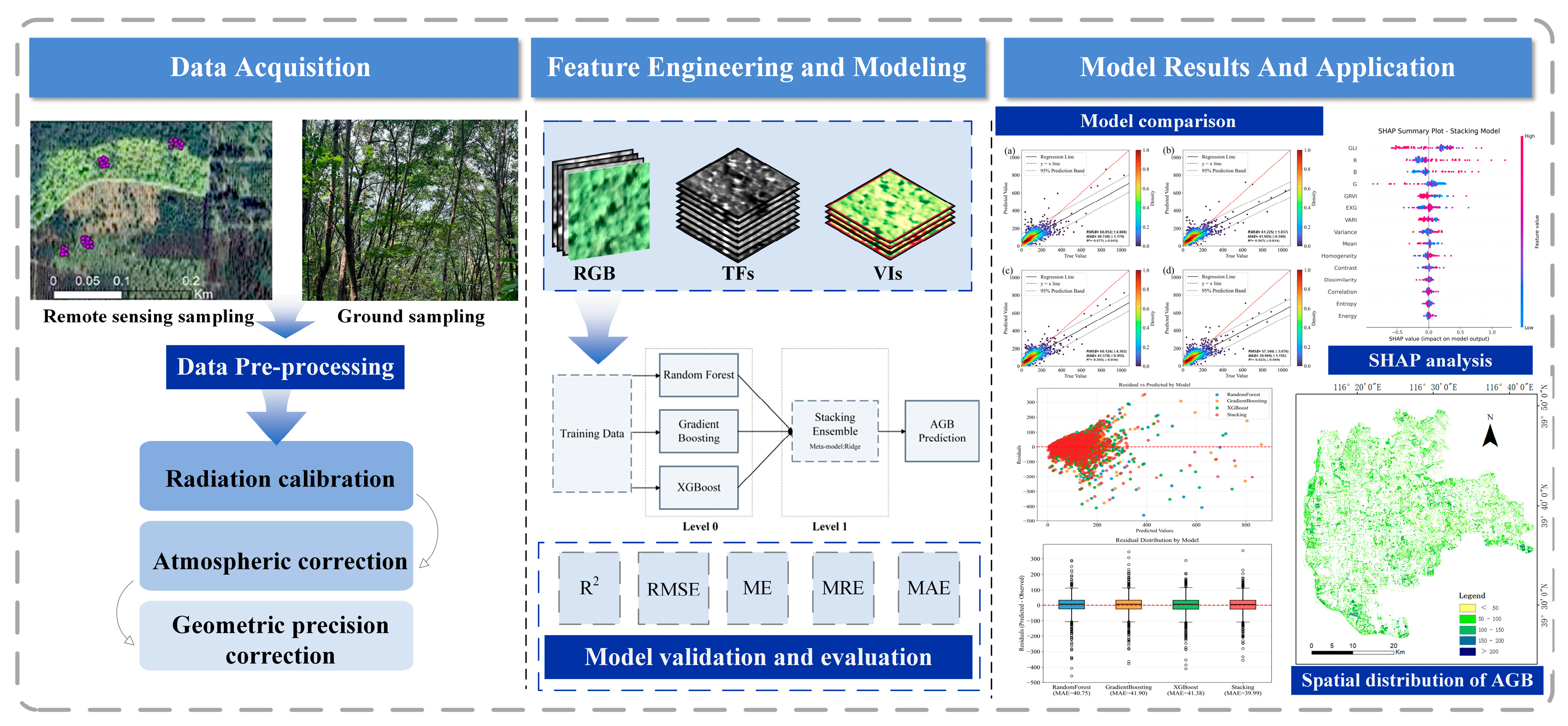
Figure 1. Workflow of the Data Processing. (Model fitting results: (a) RF, (b) GBT, (c) XGBoost, and (d) Stacking ensemble).
Forests 16 01777 g001
Figure 2. The spatial distribution dataset of AGB values in the study area sample plots.
Forests 16 01777 g002
Figure 3. Stacking ensemble learning workflow.
Forests 16 01777 g003
Figure 4. Distribution of AGB by DBH Size Groups.
Forests 16 01777 g004
Figure 5. Model fitting results: (a) RF, (b) GBT, (c) XGBoost, and (d) Stacking ensemble.
Forests 16 01777 g005
Figure 6. (a) Residual Distribution by model, (b) Residual vs. predicted by model.
Forests 16 01777 g006
Figure 7. Normal Q-Q plots for standardized residuals of each model. (a) RF, (b) GBT, (c) XGBoost, and (d) Stacking ensemble. Blue dots represent the standardized residuals, and the red line indicates the theoretical normal distribution. Points falling close to the red line suggest the residuals follow a normal distribution.
Forests 16 01777 g007
Figure 8. SHAP algorithm screening of important prediction results: (a) SHAP summary plot for Stacking ensemble, and (b) pie chart showing the proportion of each variable.
Forests 16 01777 g008
Figure 9. Comparison of the R2 and MAE across different models.
Forests 16 01777 g009
Figure 10. Spatial distribution of forest above-ground biomass (AGB) in Daxing District.
Forests 16 01777 g010
Table 1. The basic statistics of the sample plots of field surveys.
VariablesDBH (cm)H (m)AGB (Mg/ha)
MAX47.9029.101028.98
MIN5.042.006.39
MEAN14.439.99112.95
Standard deviation5.774.4393.95
Standard error0.160.122.56
Note: Statistics are based on 1344 sample plots. Means are reported with standard errors (SE), standard deviations (SD), minima, and maxima are provided for context. AGB is log-transformed (ln) in all modeling to stabilize variance, Table 1 displays untransformed values for interpretability.
Table 2. GLCM-based texture measures and their mathematical formulas.
Texture IndicesFormula
Mean M E A = j , k = 0 n 1 j · Q j , k
Homogeneity H O M = j , k = 0 n 1 Q j , k 1 + j k 2
Dissimilarity D I S = j , k = 0 n 1 Q j , k j k
Entropy E N T = j , k = 0 n 1 Q j , k l n Q j , k
Second Moment S E C = j , k = 0 n 1 Q j , k 2
Correlation C O R = j , k = 0 n 1 j μ j k μ k Q j , k σ j σ k
Contrast C O N = j , k = 0 n 1 Q j , k j k 2
Variance V A R = j , k = 0 n 1 Q j , k j μ j 2
The indices j and k represent the row and column positions in the GLCM, respectively, where Q j , k denotes the normalized frequency of a co-occurring pixel pair at positions j , k ; n is the number of gray levels. For the correlation formula: μ j = j , k j · Q j , k and μ k = j , k k · Q j , k are the means, while σ j = j , k j μ j 2 Q j , k and σ k = j , k k μ k 2 Q j , k are the standard deviations along the row and column directions, respectively.
Table 3. Visible-band Vegetation Indices.
Index TypeIndex NameFormulaReferences
Vegetation indicesExcess-green (EXG) 2 G R B [31]
Vegetation indicesGreen Leaf Index (GLI) 2 G R B 2 G + R + B [32]
Vegetation indicesGreen-Red Vegetation Index (GRVI) G R G + R [33]
Visible Atmospherically Resistant IndexVisible Atmospherically Resistant Index (VARI) G R G + R B [34]
Where R, G and B denote the normalized red, green, and blue band values, respectively. The values of R, G, and B range from 0 to 1.
Table 4. Model performance metrics with 95% confidence intervals.
ModelR2 (95% CI)RMSE (95% CI)MAE (95% CI)
RF0.58 (0.54–0.61)60.85 (47.28–74.42)40.75 (37.48–44.02)
GBT0.57 (0.47–0.66)61.23 (56.13–66.33)41.90 (40.27–43.53)
XGBoost0.59 (0.49–0.68)60.12 (48.18–72.06)41.38 (38.73–44.03)
Stacking 0.62 (0.49–0.76)57.34 (47.14–67.54)39.99 (36.79–43.19)
Notes: Values are presented as mean (95% CI).
Disclaimer/Publisher’s Note: The statements, opinions and data contained in all publications are solely those of the individual author(s) and contributor(s) and not of MDPI and/or the editor(s). MDPI and/or the editor(s) disclaim responsibility for any injury to people or property resulting from any ideas, methods, instructions or products referred to in the content.