Article

Structural Optimization of Windbreak and Sand-Fixing Forests: A Wind Tunnel Study

1
Institute of Desertification Studies, Xinjiang Academy of Forestry, Urumqi 830063, China
2
Jinghe Desert Ecosystem Research Station, Jinghe 833303, China
3
Key Laboratory of Oasis Ecology, College of Ecology and Environment, Xinjiang University, Ministry of Education, Urumqi 830017, China
4
Technical Innovation Center for Desert–Oasis Ecology Monitoring and Restoration, Ministry of Natural Resources, Urumqi 830002, China
5
College of Forestry and Landscape Architecture, Xinjiang Agricultural University, Urumqi 830052, China
*
Author to whom correspondence should be addressed.
Forests 2025, 16(11), 1710; https://doi.org/10.3390/f16111710
Submission received: 16 September 2025 / Revised: 5 October 2025 / Accepted: 16 October 2025 / Published: 10 November 2025
(This article belongs to the Section Forest Ecology and Management)

Abstract

This study examined the windbreak effects of different tree–shrub configurations through wind tunnel experiments. Using Populus euphratica Oliv. and Tamarix chinensis Lour. as model species, six rows of front-tree–back-shrub arrangements in a triangular layout were tested under varying spacing patterns. Four spacings of P e (7.5 cm × 7.5 cm, 7.5 cm × 10 cm, 7.5 cm × 12.5 cm, 10 cm × 10 cm) and four spacings of T cs (5 cm × 5 cm, 5 cm × 7.5 cm, 5 cm × 10 cm, 7.5 cm × 7.5 cm) were analyzed. Tree–shrub combinations significantly outperformed pure stands. The configuration of P e (7.5 cm × 10 cm) with T c (5 cm × 10 cm) achieved the highest efficiency, with an average of 27.1% and a peak of 47.13% at 7 H. This configuration was effective up to 15 H and showed slower efficiency decline at higher wind speeds. Vertically, most combinations reached maximum efficiency at 20 cm height, while pure T c peaked at 51.96% at 3 cm and pure P e at 36.33% at 20 cm. Overall, the optimal configuration was P e spaced at 7.5 cm × 10 cm and T c at 5 cm × 10 cm, which not only enhanced protective performance but also reduced planting density. These findings provide valuable scientific references for designing windbreak and sand-fixing forests in arid regions, supporting ecological restoration and sustainable land management in desert–oasis transition zones.

1. Introduction

Oases are distinctive ecosystems in arid and semi-arid regions, playing a vital role in maintaining the balance among water, soil, air, and biodiversity. They are also critical to the sustainable development of human settlements in these fragile environments. Among the major ecological components of oases, windbreak and sand-fixing forests are particularly important [1,2]. These vegetation systems effectively reduce wind velocity, limit sand transport, and suppress the spread of desertification. Establishing shelterbelts around oasis peripheries not only mitigates the intensity of sandstorms but also improves the quality of local living environments [3,4].
Over the past decades, extensive studies have been conducted to explore the configuration and function of windbreak and sand-fixing forests. These investigations have used field observations [5,6,7], wind tunnel experiments [8], and numerical simulations [9] to assess their aerodynamic behavior. The protective efficiency of shelterbelts depends on several structural factors, including stand density [10], tree and row spacing [11,12], species composition [13], porosity [14], and strip width [15]. Generally, greater vegetation height and wider forest belts extend the protective distance [16]. Porosity, defined as the proportion of internal pore space relative to the total vegetation volume, has a crucial influence on airflow regulation [17]. High porosity allows stronger wind penetration and shortens the protective range, while excessively low porosity increases resistance but induces leeward vortex formation, also reducing the overall efficiency [18,19]. Therefore, an optimal porosity exists that balances aerodynamic resistance and flow stability [17,20].
Species composition is another key determinant of forest performance. Mixed windbreaks composed of trees, shrubs, and grasses create vertically stratified structures that enhance shelter efficiency and ecological stability [21]. The airflow structure is also strongly influenced by the spatial configuration of forest strips. Building upon Judd [22], Mayaud [23] divided the airflow field around individual trees into six zones: the windward, displacement acceleration, seepage, calm, mixing, and rebalancing zones. Further studies identified additional vertical layers, including the mixed layer [24], internal canopy zone [25], and near-surface zone [26]. Horne [27] proposed a two-part wake model, dividing it into near-wake and far-wake regions. The near-wake is characterized by strong turbulence and velocity deficits, whereas in the far-wake, turbulence gradually decays and velocity recovers. The extent of wake dissipation largely depends on vegetation morphology and spatial arrangement.
However, most previous research has focused on single-species windbreaks, which, although effective during early growth stages, often lose stability and protection efficiency over time due to plant mortality and canopy fragmentation. Studies addressing multi-species compositions, optimal spacing, and structural configurations remain limited. In arid zones, selecting native, drought- and salt-tolerant species with deep root systems and strong sand-fixing capacity is essential for maintaining long-term stability and ecological resilience of windbreak systems.
Populus euphratica Oliv. and Tamarix chinensis Lour. are two dominant native species widely used in afforestation projects across Xinjiang. They exhibit strong adaptability to arid conditions and serve as ideal candidates for windbreak and sand-fixation forests. This study focuses on the combined use of these species under controlled conditions. Through systematic wind tunnel experiments, various row-spacing combinations were tested to evaluate wind speed attenuation, flow field distribution, and protection efficiency. The results aim to determine the optimal spacing and configuration mode for maximizing shelter performance. Ultimately, this research provides a practical reference for optimizing the design of windbreak and sand-fixing forests in arid and semi-arid regions, contributing to both ecological restoration and sustainable land management.

2. Materials and Methods

2.1. Experimental Equipment

The wind tunnel experiments were conducted from May to June 2025 at the “Wind and Sand Environment Wind Tunnel Laboratory” of the Gansu Desertification Research Institute. The wind tunnel used was a non-circulating type with an adjustable wind speed range of 4–35 m s−1. The total length of the wind tunnel was 38.9 m and consisted of an inlet section, power section, rectifying section, contraction section, test section, adjustable test section, and diffusion section. The test section had a length of 16 m, with a cross-sectional area of 1.2 m (width) × 1.2 m (height), and the adjustable section was 2.5 m long. The boundary layer thickness (V = 0.99V) in the wind tunnel was approximately 30 cm, which was larger than the height of the plant models, meeting the requirement that the experimental model must be fully within the wind tunnel boundary layer (Figure 1). To ensure the reliability of the results, the simulation required geometric similarity, kinematic similarity, and dynamic similarity. Roughness elements (wooden boards with streamlined edges) were added in the wind tunnel to stabilize airflow and prevent boundary layer separation.

2.2. Experimental Materials

The most critical requirement for the wind tunnel simulation was to ensure the models adhered to geometric similarity, meaning they closely resembled the real plant forms in proportion. All physical parameters were nondimensionalized, and the physical relationships were compared without considering the units. The experimental materials included models of Populus euphratica Oliv. (P e) and Tamarix chinensis Lour. (T c). Before the wind tunnel tests, field surveys of typical mature P e and T c were conducted to determine key parameters such as trees height and crown width. Considering the influence of the boundary layer on accuracy, the dimensions of the models were scaled at a ratio of 1:40. The model for P e had a height of 30 cm and a crown width of 10 cm × 10 cm, while the model for T c was 6 cm tall with a 6 cm × 6 cm crown width. The blockage area of the model was kept under 5% of the test section’s cross-sectional area to satisfy the geometric similarity requirements. The plant models were fixed on foam boards as shown in Figure 2.

2.3. Model Design

The study used a fan-shaped layout model with six rows of trees, simulating a configuration of three rows of P e in the front and three rows of T c in the back. The plant spacing for P e, based on actual distances of 3 m × 3 m, 3 m × 4 m, 3 m × 5 m, and 4 m × 4 m, was scaled proportionally to 7.5 cm × 7.5 cm, 7.5 cm × 10 cm, 7.5 cm × 12.5 cm, and 10 cm × 10 cm, respectively. For T c, the plant spacing, based on actual distances of 2 m × 2 m, 2 m × 3 m, 2 m × 4 m, and 3 m × 3 m, was scaled proportionally to 5 cm × 5 cm, 5 cm × 7.5 cm, 5 cm × 10 cm, and 7.5 cm × 7.5 cm, respectively. The specific configurations are shown in Table 1.

2.4. Wind Speed Measurement

Wind speed was measured using Pitot tubes, with the wind pressure converted to wind speed by differential pressure sensors. Data were recorded by a data acquisition system. At each measurement point, at least 80 instantaneous wind speed readings were taken over a duration of approximately 40 s, with two readings per second. The average value of the data was used for analysis. Three wind speeds (6, 10 and 15 m s−1) were tested, and measurements were taken along the central axis from 3H ahead of the forest belt to 15H behind it at 13 measurement points. Wind speed was recorded at nine heights (1, 3, 5, 8, 13, 20, 30, 40, and 60 cm), with H representing the average height of the plant models (H = 18 cm for the average trees height of P e and T c, H = 30 cm for P e, and H = 6 cm for T c). The measurement positions are shown in Figure 3.

2.5. Data Processing

2.5.1. Relative Wind Speed Calculation

Relative wind speed is a key parameter that reflects the acceleration and deceleration of wind caused by the windbreak. In this experiment, changes in relative wind speed around different models were used to assess the varying effects of different windbreak and sand-fixing forest configurations on wind speed. The relative wind speed was classified into three zones: ① Deceleration Zone: (0, 0.6] ② Transition Zone: (0.6, 1] ③ Acceleration Zone: >1 [10,28,29]. Based on wind speed measurements taken in the wind tunnel, both with and without a windbreak, the wind speeds at each measurement point were standardized. The formula for calculating relative wind speed is as follows:
A = U U 0
In the equation: A represents the relative wind speed; U refers to the wind speed measured in the presence of the windbreak (m s−1); and U0 refers to the wind speed measured in the absence of the windbreak (m s−1).

2.5.2. Windbreak Efficiency

Windbreak efficiency is an important indicator reflecting the wind protection benefits of different windbreak and sand-fixing forest models. Its calculation is shown in Equation (2).
E wind = ( V open   -   V measure ) / V open × 100 %
where
  • Ewind—Windbreak efficiency;
  • Vopen—Average wind speed at height Z in the open area (m s−1);
  • Vmeasure—Average wind speed at height Z at a distance of h from the windbreak (m s−1)

2.5.3. Data Analysis and Mapping

The data were processed using Surfer 15.0 software to plot wind speed and windbreak effectiveness contour maps. Origin 2019 software was used for statistical analysis and chart plotting.

3. Results and Analysis

3.1. Initial Wind Field Analysis Without the Model

The quality of the initial flow field in the wind tunnel determines the reliability of the test simulation results. To ensure consistency in the initial flow field during wind tunnel tests, each wind speed test was conducted for a uniform duration of 40 s. After averaging the obtained wind speeds, the corresponding wind speeds at different heights for various wind speeds are shown in Table 2. At different wind speeds, wind speed exhibits a good logarithmic relationship with height, allowing wind speed values at any height to be inferred using the wind speed profile equation.

3.2. Flow Field Characteristics of Different Tree-Shrub Windbreak and Sand-Fixing Forests

3.2.1. Flow Field Analysis of Different Tree-Shrub Windbreak and Sand-Fixing Forests at 6 m s−1

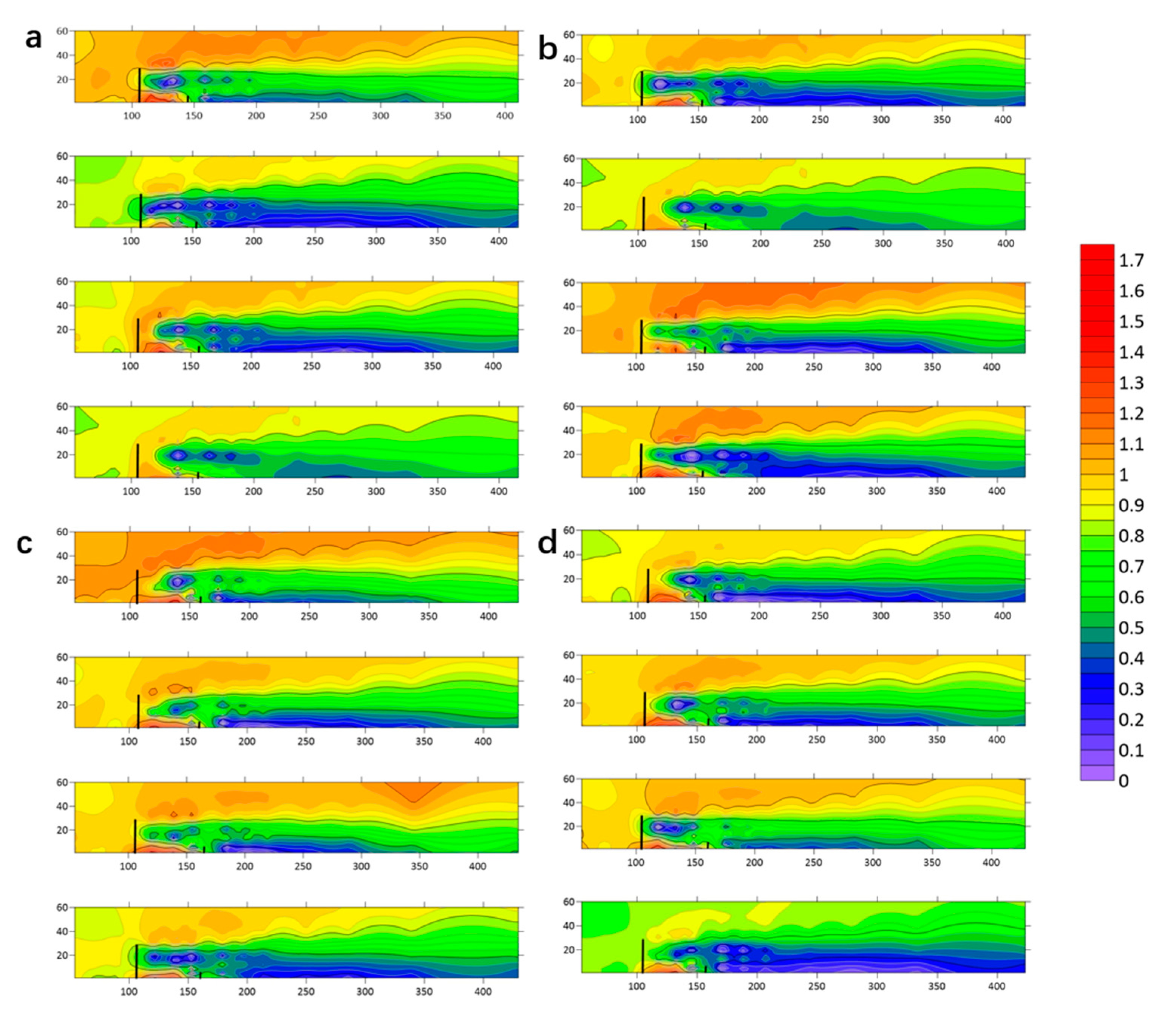
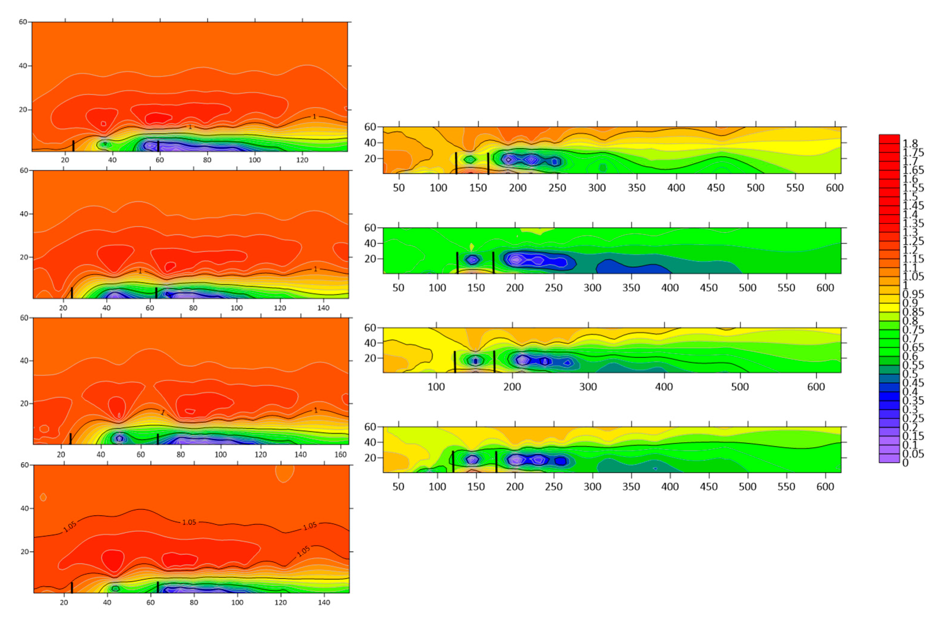
When wind speed reaches 6 m s−1, the relative wind speed contour maps for different configurations of tree-shrub windbreak and sand-fixing forests are shown in Figure 4 and Figure 5. A higher U/U0 ratio indicates more pronounced wind acceleration and poorer windbreak effectiveness. The wind shadow zones and acceleration zones differ across each model. The wind speed attenuation zone for the tree-shrub combination (U/U0 = (0, 0.6]) is larger than that for pure P e or pure T c stands. Wind acceleration becomes more pronounced with increasing height. When P e spacing was 7.5 cm × 7.5 cm and T c spacing was 5 cm × 7.5 cm, the wind speed reduction effect was most pronounced (23.58%). Conversely, the wind acceleration zone was largest (39.57%) when P e spacing was 7.5 cm × 7.5 cm and T c spacing was 5 cm × 5 cm. When P e were planted at 7.5 m × 10 m spacing and combined with T c at 5 m × 5 m spacing, wind speed reduction was most pronounced (24.56%); the greatest wind acceleration zone occurred with P e at 7.5 m × 10 m spacing and T c at 5 m × 10 m spacing (22.57%); When P e spacing was 7.5 cm × 12.5 cm, the tree-shrub combination of T c at 5 cm × 5 cm showed the most pronounced wind speed reduction (21.25%); with P e spacing at 7.5 cm × 12.5 cm and T c at 5 cm × 7.5 cm, the wind acceleration zone was largest (34.78%); When P e spacing was 10 cm × 10 cm, the tree-shrub combination of T c (5 cm × 7.5 cm) showed the most pronounced wind speed reduction (16.71%); with P e spacing at 10 cm × 10 cm andT c spacing at 5 cm × 5 cm, the wind acceleration zone was largest (31.82%). At 6 m s−1, the most pronounced wind speed reduction among all tree–shrub combinations occurred in the P e 7.5 cm × 10 cm × T c 5 cm × 5 cm configuration. Among T c-based combinations, the most significant wind reduction was observed in the 5 cm × 10 cm spacing pattern. Among P e combinations, the 7.5 cm × 7.5 cm spacing pattern exhibited the most pronounced wind speed reduction.

3.2.2. Flow Field Analysis of Different Tree-Shrub Windbreak and Sand-Fixing Forests at 10 m s−1

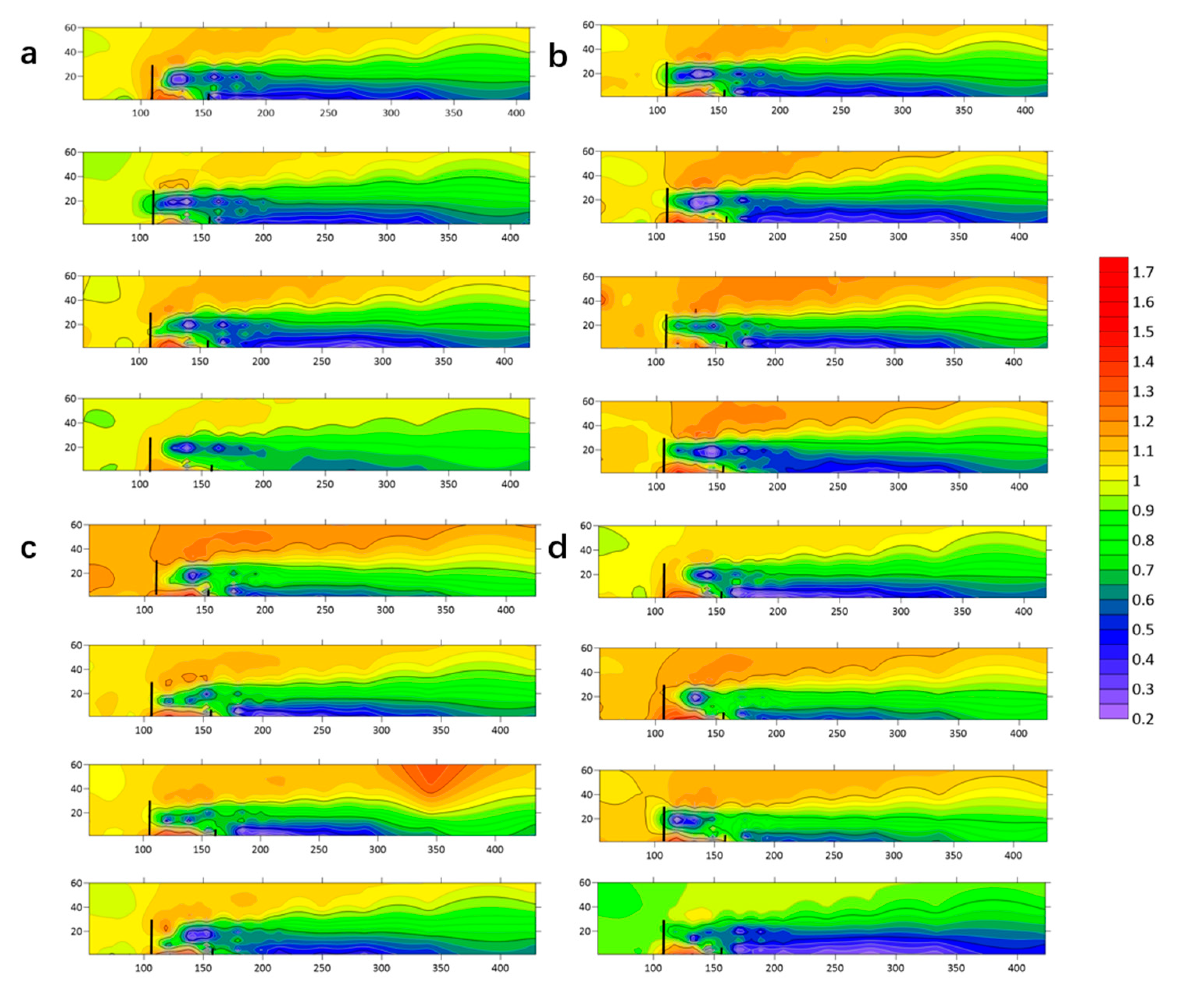
When wind speed reaches 10 m/s, the relative wind speed contour lines for different configurations of tree–shrub windbreak and sand-fixing forests are shown in and Figure 6 and Figure 7. As wind speed increases, the wind speed reduction zone gradually decreases. When the spacing of P e is 7.5 cm × 7.5 cm, the combination with T c at 5 cm × 5 cm demonstrates the most significant wind speed reduction (21.45%), while the combination with T c. at 7.5 cm × 7.5 cm exhibits the largest wind speed acceleration zone (45.37%). When the spacing of P e is 7.5 cm × 10 cm, the combination with T c at 5 cm × 5 cm shows the greatest wind speed reduction (24.56%), while the combination with T c at 5 cm × 10 cm has the largest wind speed acceleration zone (39.46%). With P e spacing at 7.5 cm × 12.5 cm, the combination with T c at 5 cm × 5 cm yields the most substantial wind speed reduction (22.93%), while the combination with T c at 5 cm × 10 cm results in the largest wind speed acceleration zone (49.07%). At a spacing of 10 cm × 10 cm for P e, the combination with T c. at 5 cm × 5 cm shows the most notable wind speed reduction (14.56%), while the combination with T c. at 5 cm × 7.5 cm has the largest wind speed acceleration zone (45.06%).
Among all the tree–shrub combinations at 10 m s−1, the combination of P e. at 7.5 cm × 10 cm and T c. at 5 cm × 5 cm demonstrates the most significant wind speed reduction. Within the T c. configurations, the 5 cm × 10 cm spacing pattern shows the most considerable wind speed reduction, while among the P e. configurations, the 7.5 cm × 7.5 cm spacing pattern exhibits the most notable wind speed reduction.

3.2.3. Flow Field Analysis of Different Tree-Shrub Windbreak and Sand-Fixing Forests at 15 m s−1

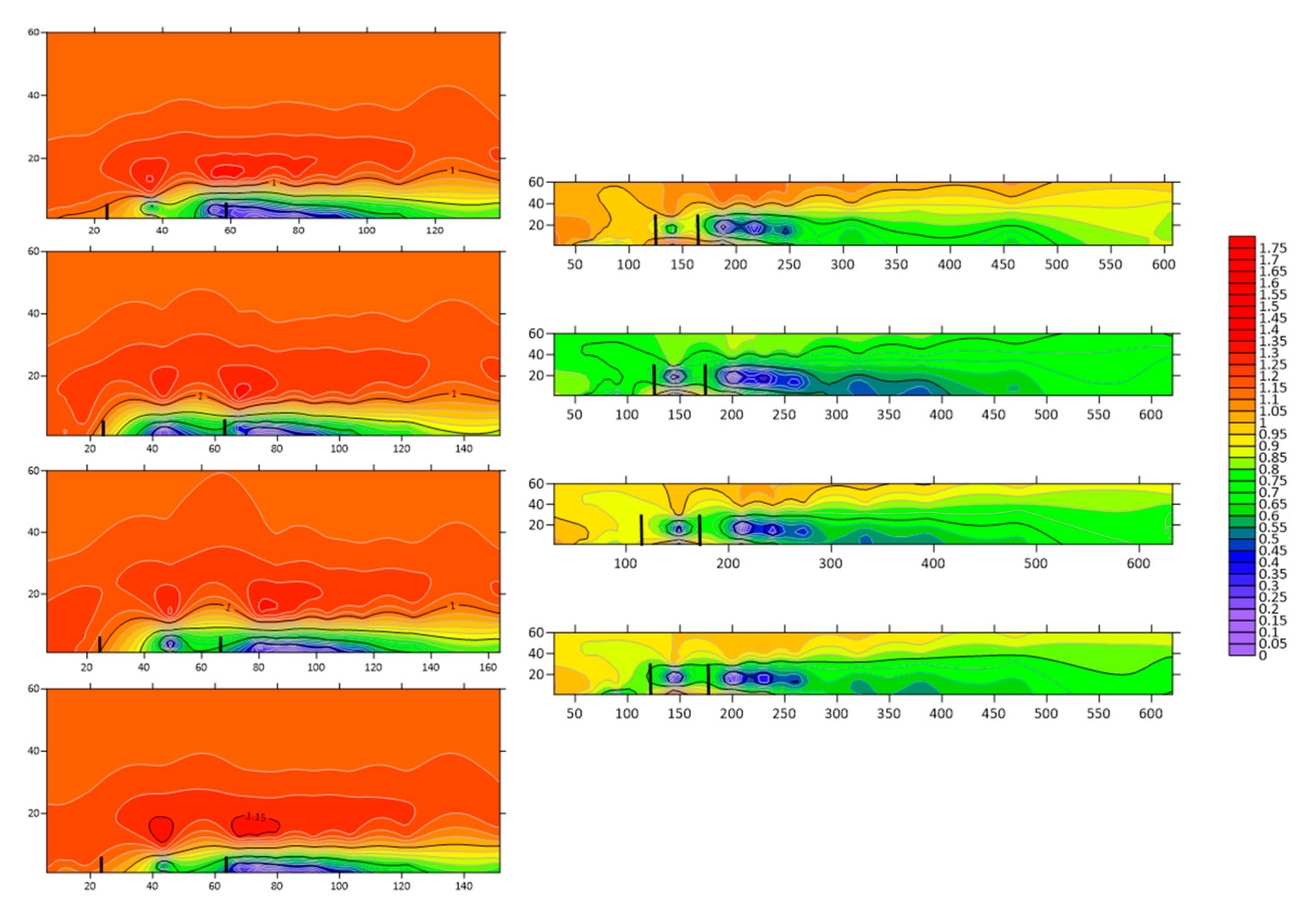
When the wind speed reaches 15 m s−1, the relative wind speed for different tree-shrub windbreak configurations is illustrated in and Figure 8 and Figure 9. As the wind speed increases, the wind speed reduction zone becomes progressively smaller. For P e. with a spacing of 7.5 cm × 7.5 cm, the combination with T c at 5 cm × 7.5 cm demonstrates the most significant wind speed reduction (14.63%), while the combination with T c at 7.5 cm × 7.5 cm shows the largest wind speed acceleration zone (46.55%). When the spacing of P e is 7.5 cm × 10 cm, the combination with T c. at 5 cm × 10 cm exhibits the greatest wind speed reduction (15.07%), along with the largest wind speed acceleration zone (44.11%). For a spacing of 7.5 cm × 12.5 cm for P e, the combination with T c at 5 cm × 5 cm shows the most significant wind speed reduction (10.90%), whereas the combination with T c. at 5 cm × 10 cm has the largest wind speed acceleration zone (52.15%). In the case of P e at 10 cm × 10 cm, the combination with T c at 5 cm × 10 cm results in the greatest wind speed reduction (11.08%), while the combination with T c at 5 cm × 5 cm shows the largest wind speed acceleration zone (45.22%).
At a wind speed of 15 m s−1, among all the tree-shrub combinations, the most significant wind speed reduction is achieved by the combination of P e at 7.5 cm × 10 cm and T c at 5 cm × 10 cm. Among the T c. configurations, the combination with a spacing of 5 cm × 10 cm shows the greatest wind speed reduction, while, for the P e configurations, the combination with a spacing of 7.5 cm × 7.5 cm exhibits the most substantial wind speed reduction.

3.3. Windbreak Efficiency Analysis of Different Tree-Shrub Windbreak and Sand-Fixing Forests

3.3.1. Windbreak Efficiency Analysis at 6 m s−1

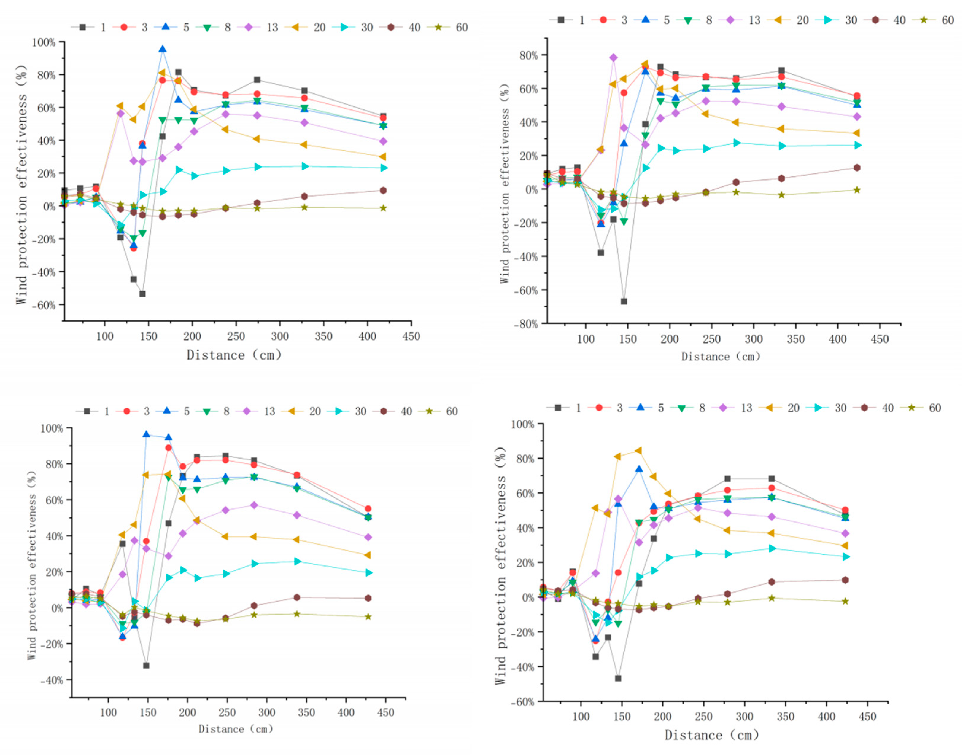
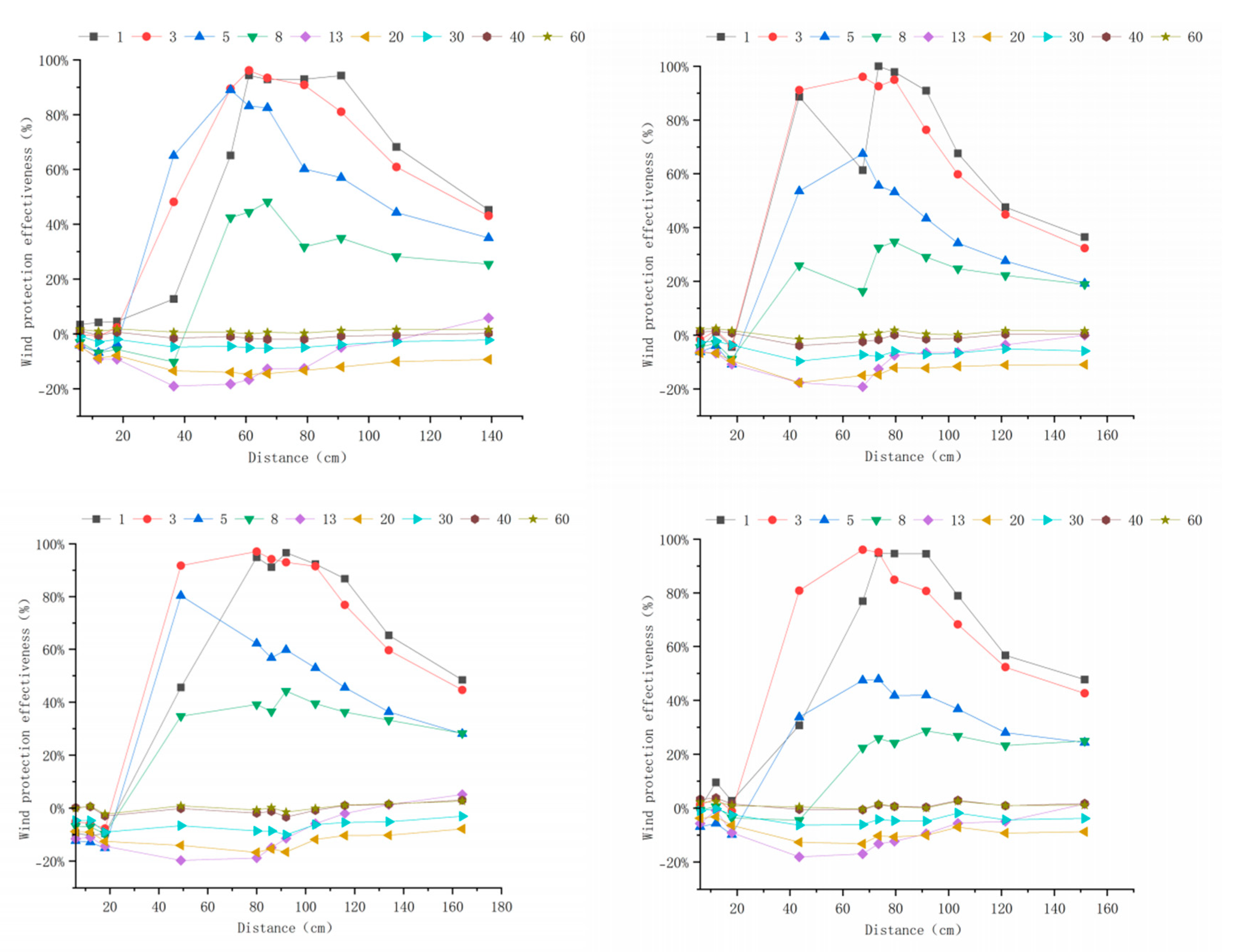
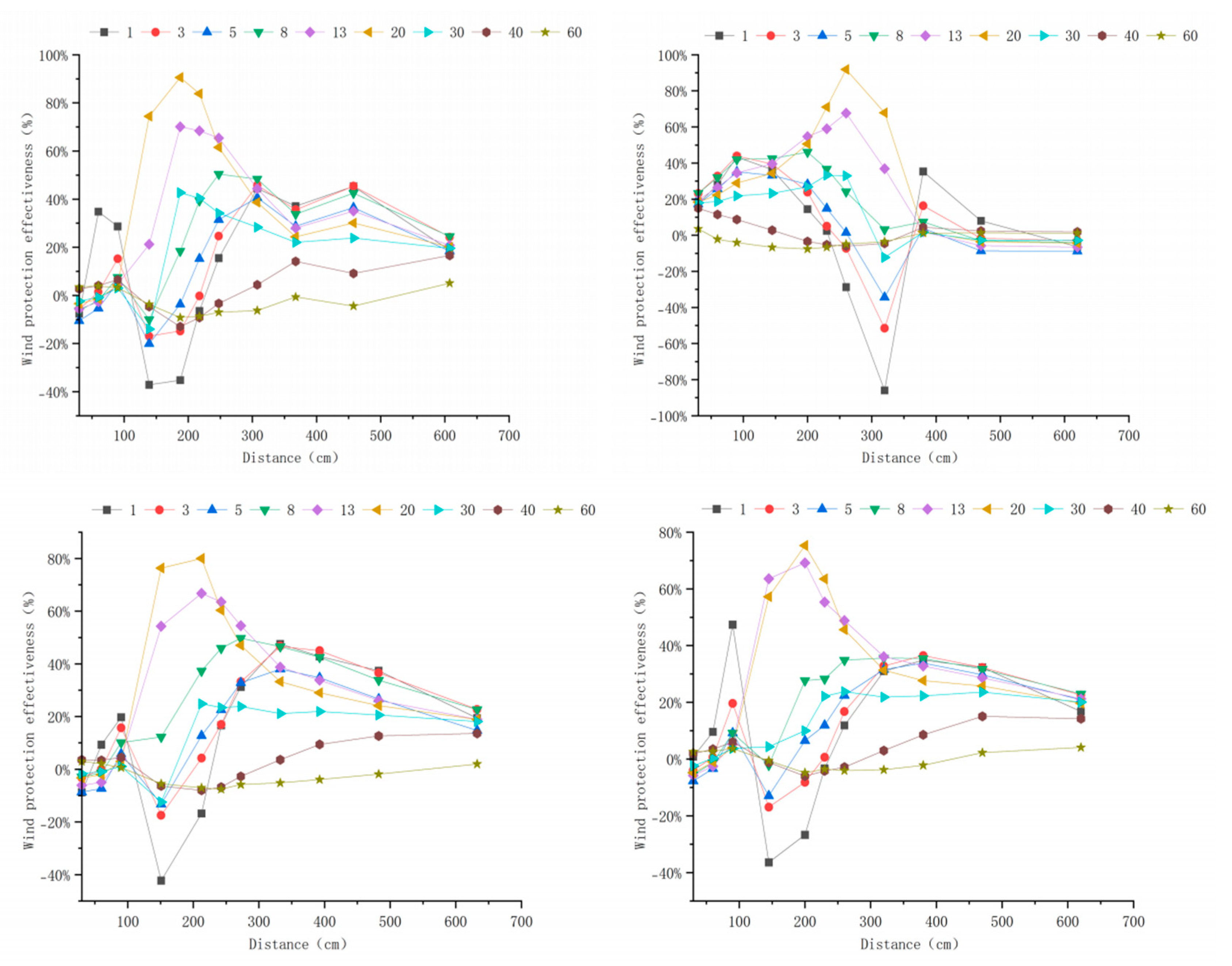
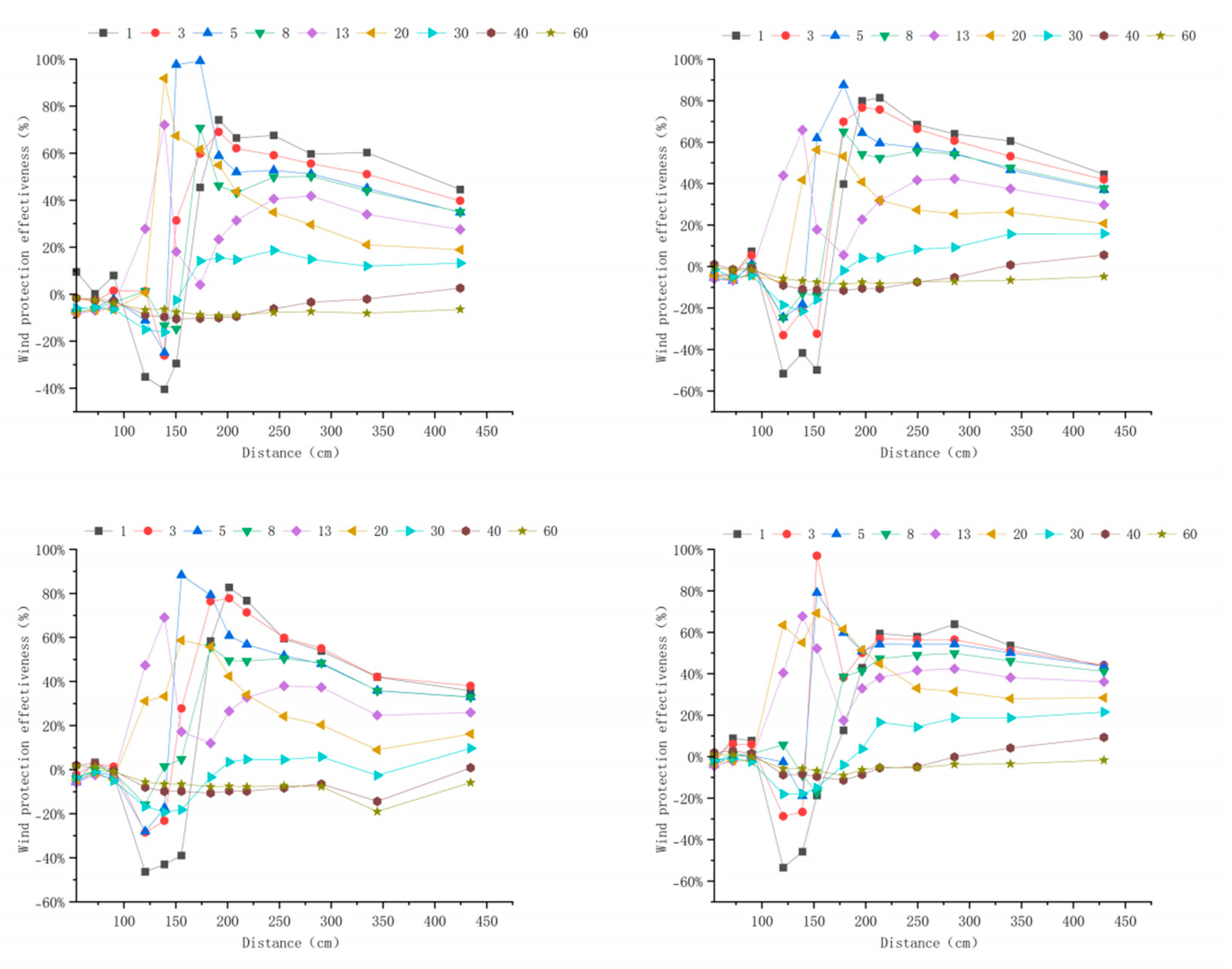
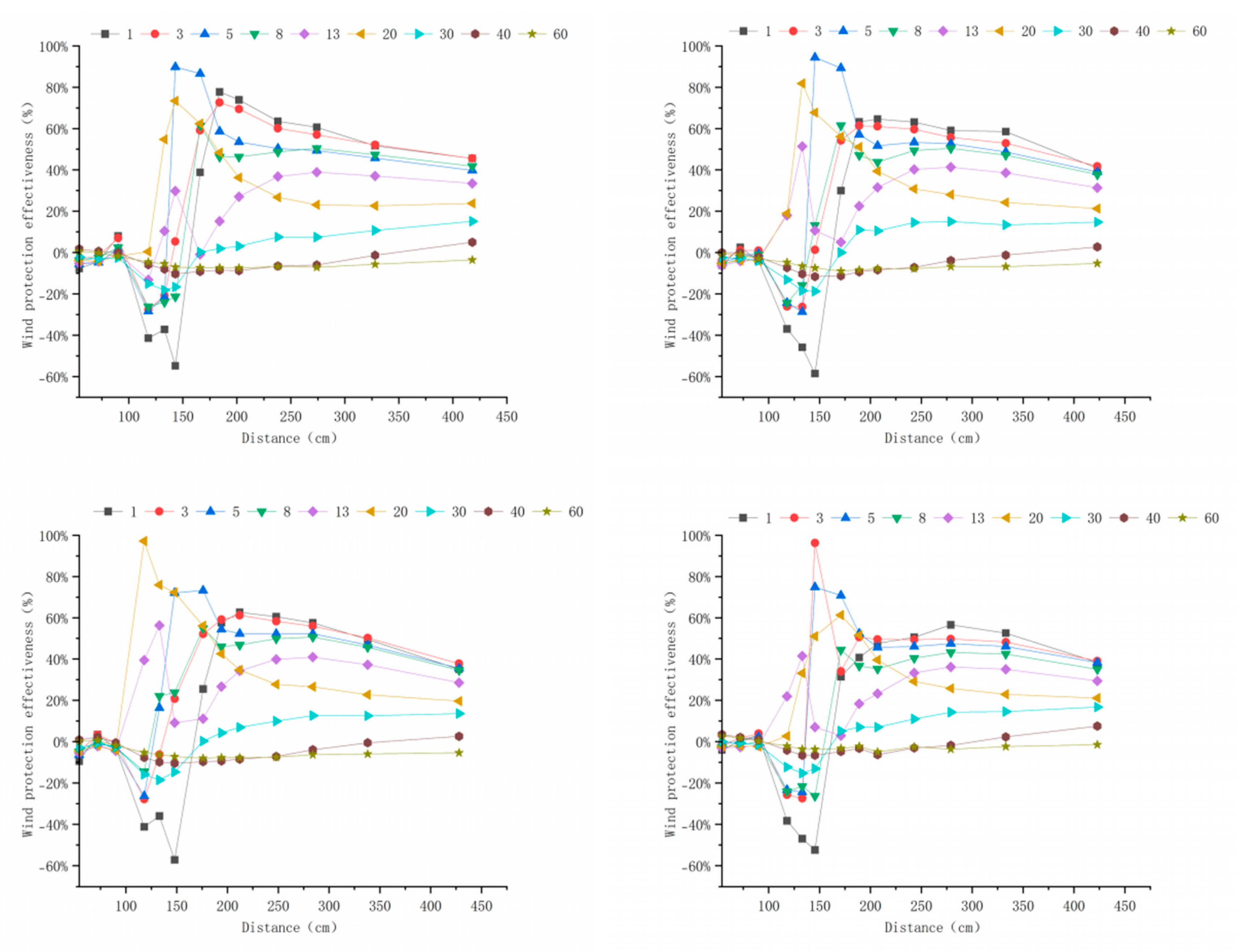
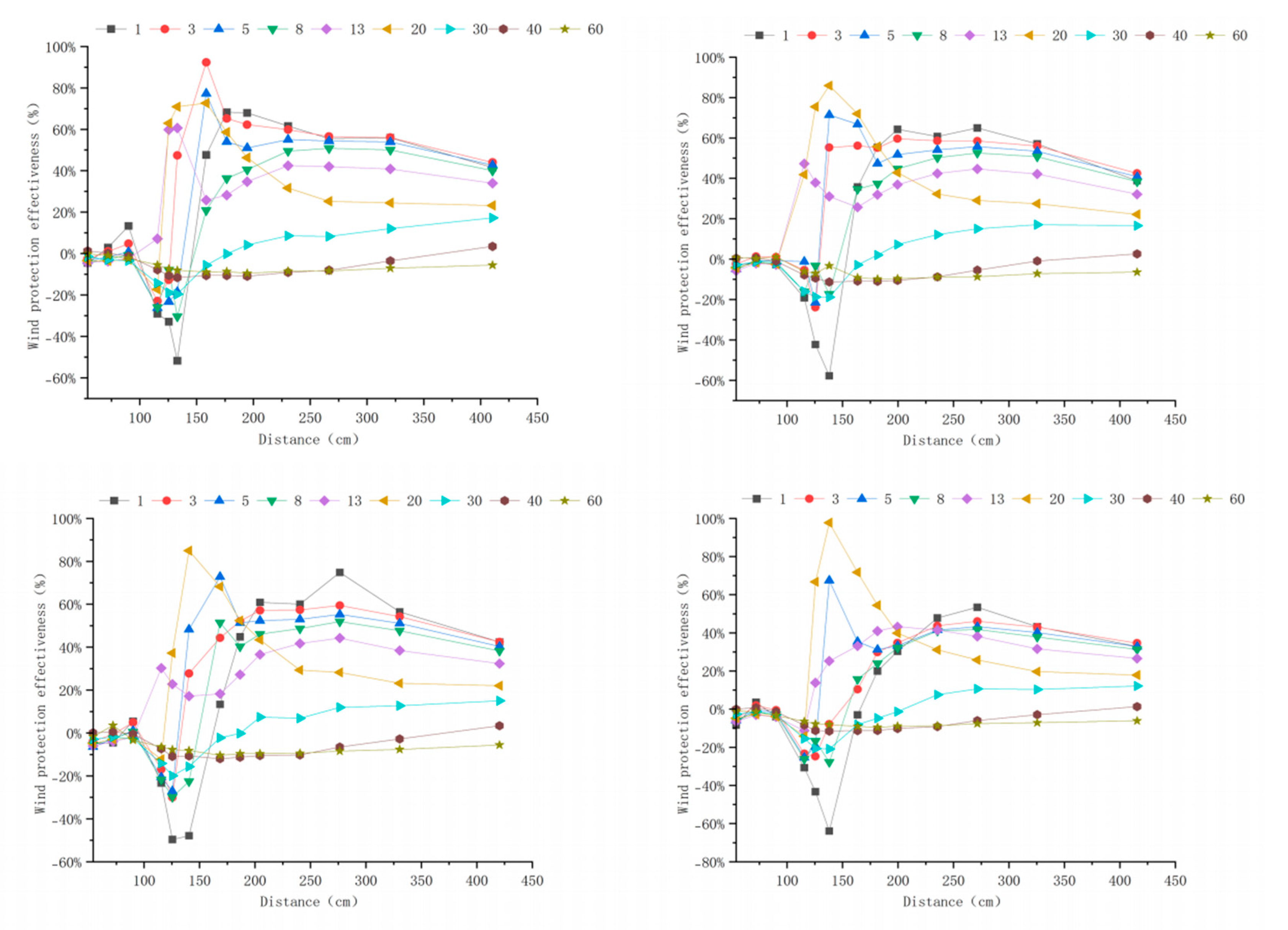
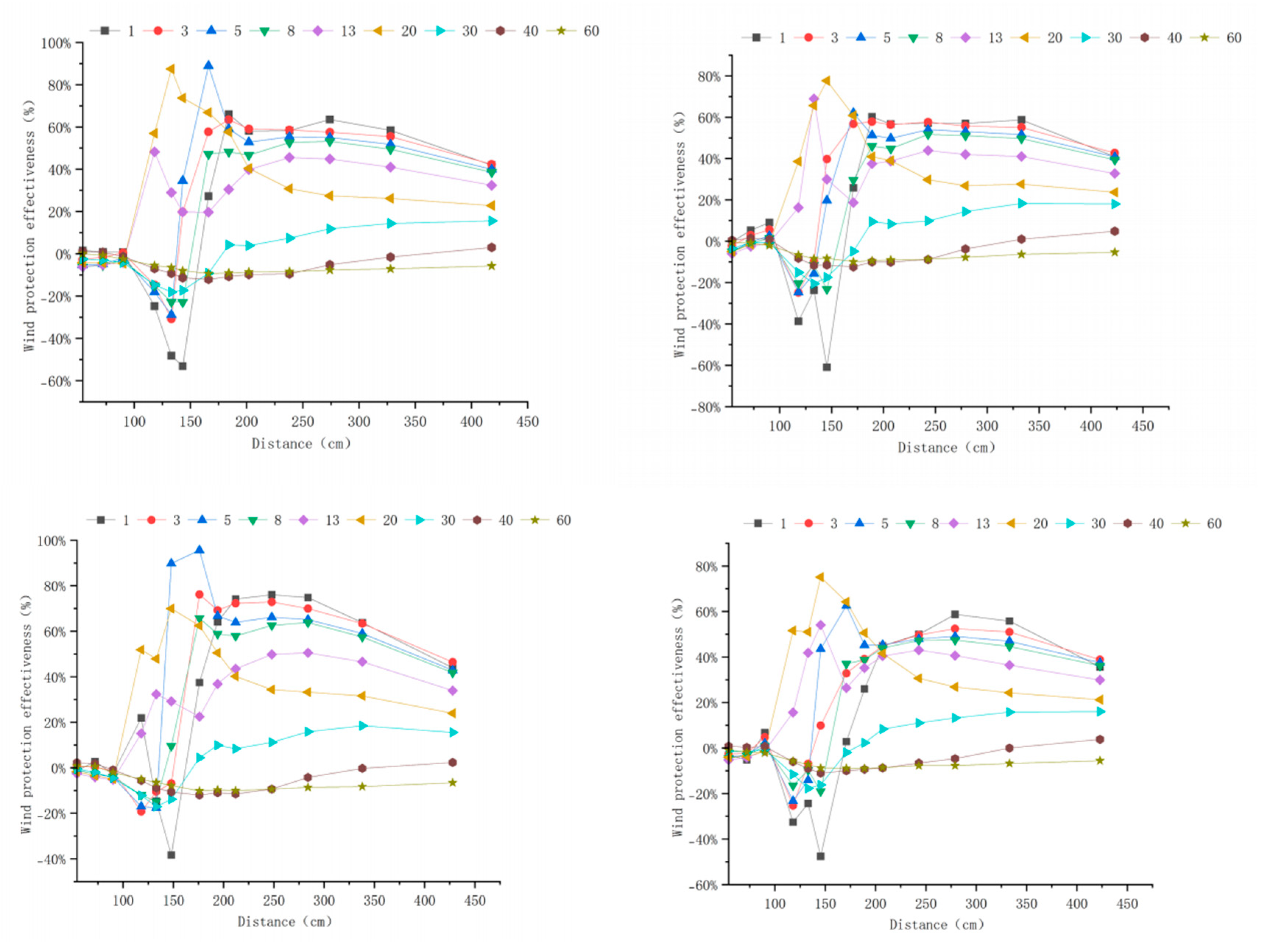
Windbreak efficiency is a key indicator for assessing the protective benefits of windbreak and sand-fixing forests (Negative efficiency indicates that wind speed in the leeward zone exceeded the reference flow, reflecting localized acceleration caused by turbulence or channeling effects within the canopy). The windbreak efficiency at 6 m s−1 is shown in Appendix A Figure A1, Figure A2, Figure A3, Figure A4, Figure A5 and Figure A6. Comparing the windbreak efficiency across multiple points and heights for different models at 6 m s−1 reveals that all models exhibited varying degrees of efficiency change between 0 and 30 cm in height. Most models achieved their maximum windbreak efficiency at a height of 20 cm, while at 40 cm and 60 cm, the efficiency remained low or negative. In terms of distance, the maximum windbreak efficiency was observed at 7H. Due to the narrow tube effect at the measurement points within the model, the windbreak efficiency values were mostly negative.
Among the different models, the “P e 7.5 cm × 10 cm, T c 5 cm × 10 cm” combination exhibited the highest average windbreak efficiency at 27.1%, surpassing all other configurations. The maximum windbreak efficiency for this combination reached 47.13% at 7H, and it maintained an efficiency of over 32% between 1H and 15H. When the row spacing of P e was 7.5 cm × 12.5 cm, its windbreak efficiency between 1H and 15H (16.63%) was notably higher than other pure P e forests. Similarly, when T c had a row spacing of 5 cm × 5 cm, its windbreak efficiency between 1H and 15H (16.83%) was significantly greater than other pure T c forests.
Regarding windbreak efficiency at different heights, most tree-shrub models reached their maximum efficiency at 1.2 times the model height (20 cm). The highest windbreak efficiency for the “P e 7.5 cm × 12.5 cm, T c 5 cm × 5 cm” combination occurred at 20 cm, with a peak value of 42.64%. For pure T c forests, due to their shorter trees height, the maximum windbreak efficiency occurred at 3 cm, with a peak value of 54.96% for the row spacing of 7.5 cm × 7.5 cm. For pure P e forests, the maximum windbreak efficiency occurred at 20 cm, with a peak value of 36.33% for the row spacing of 7.5 cm × 7.5 cm.

3.3.2. Windbreak Efficiency Analysis at 10 m s−1

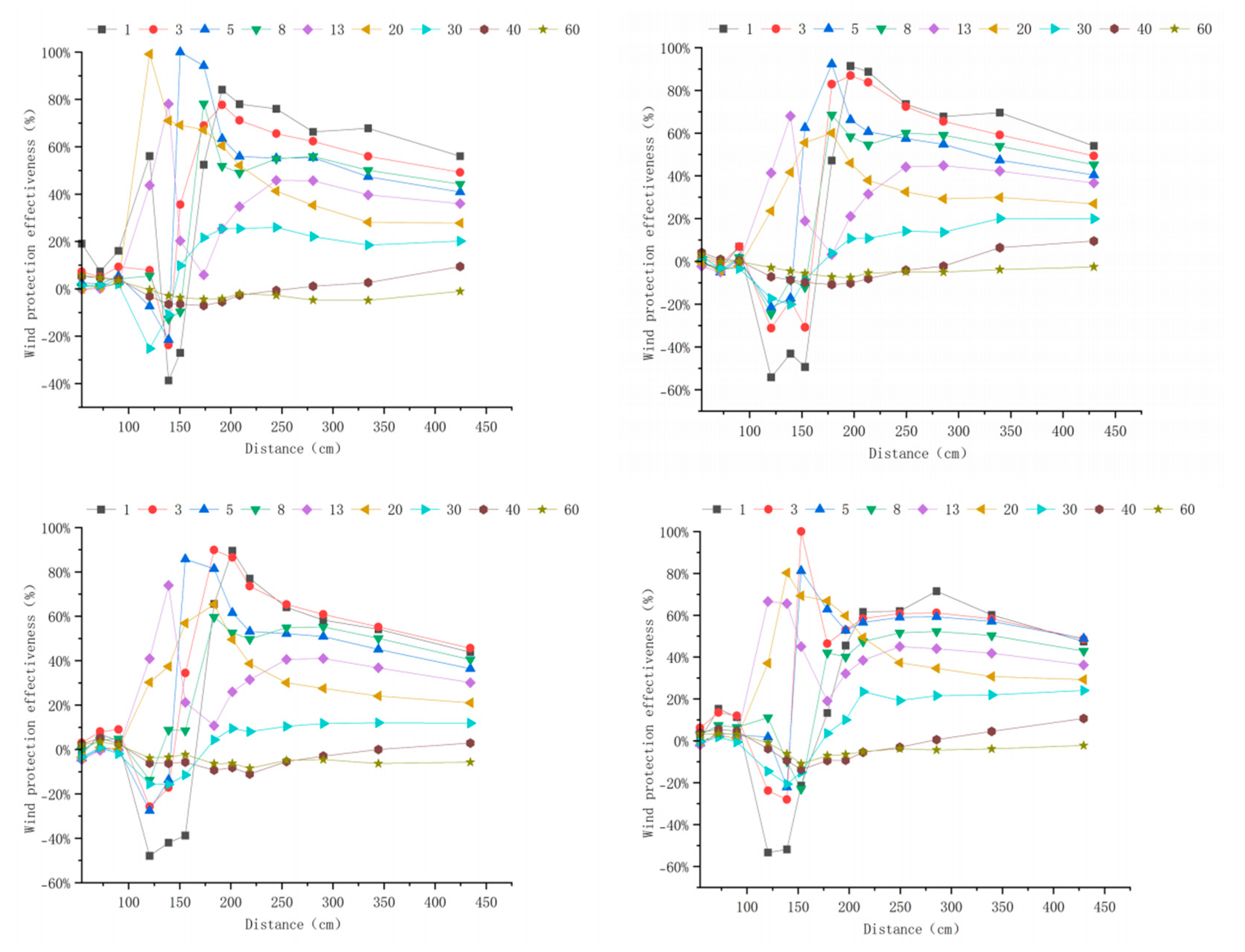
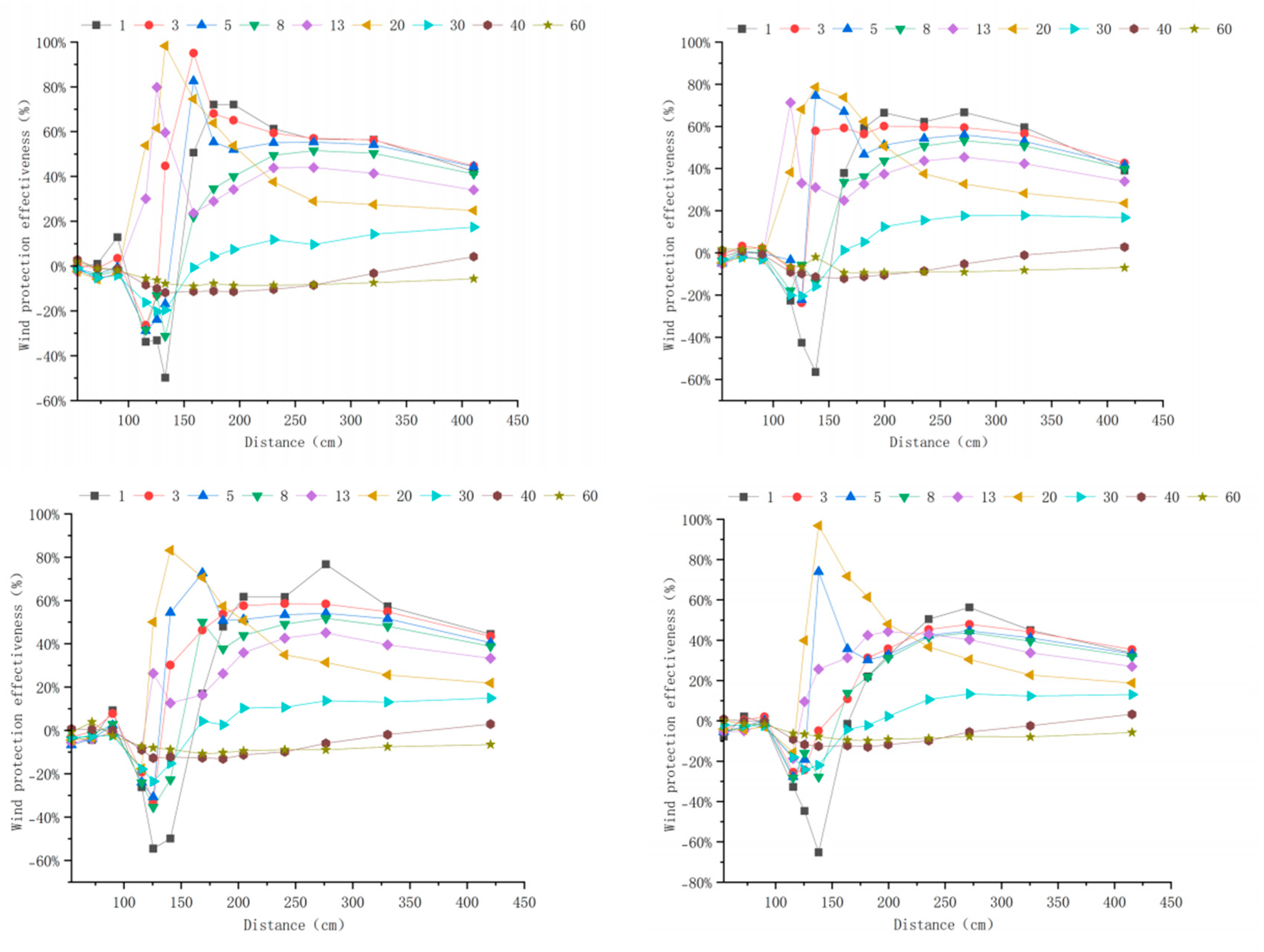
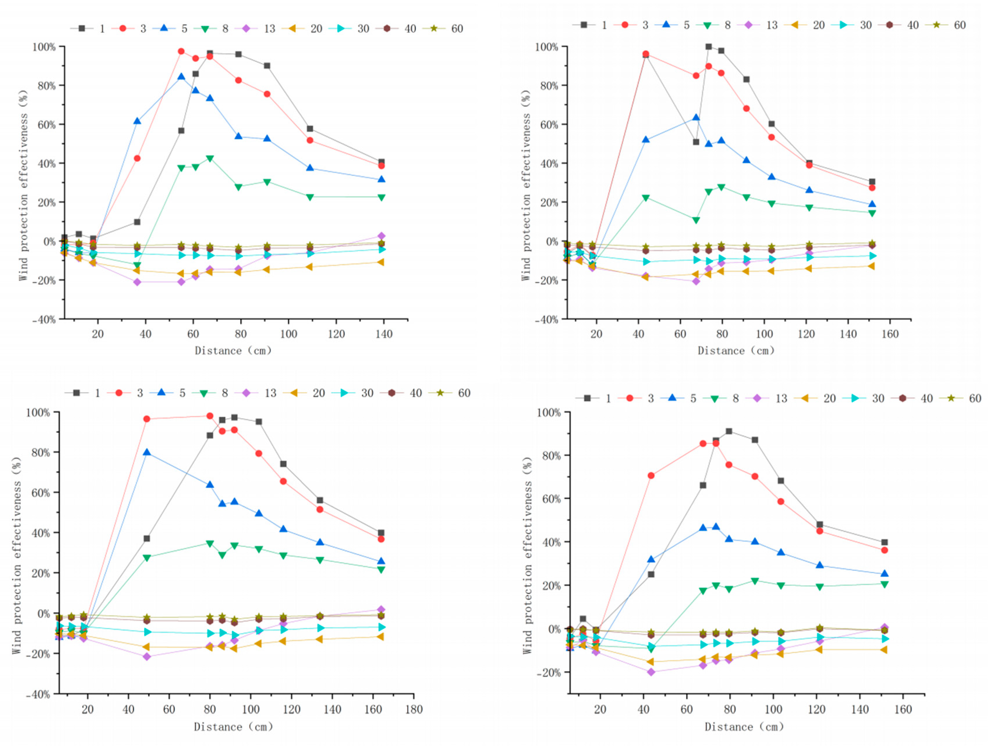
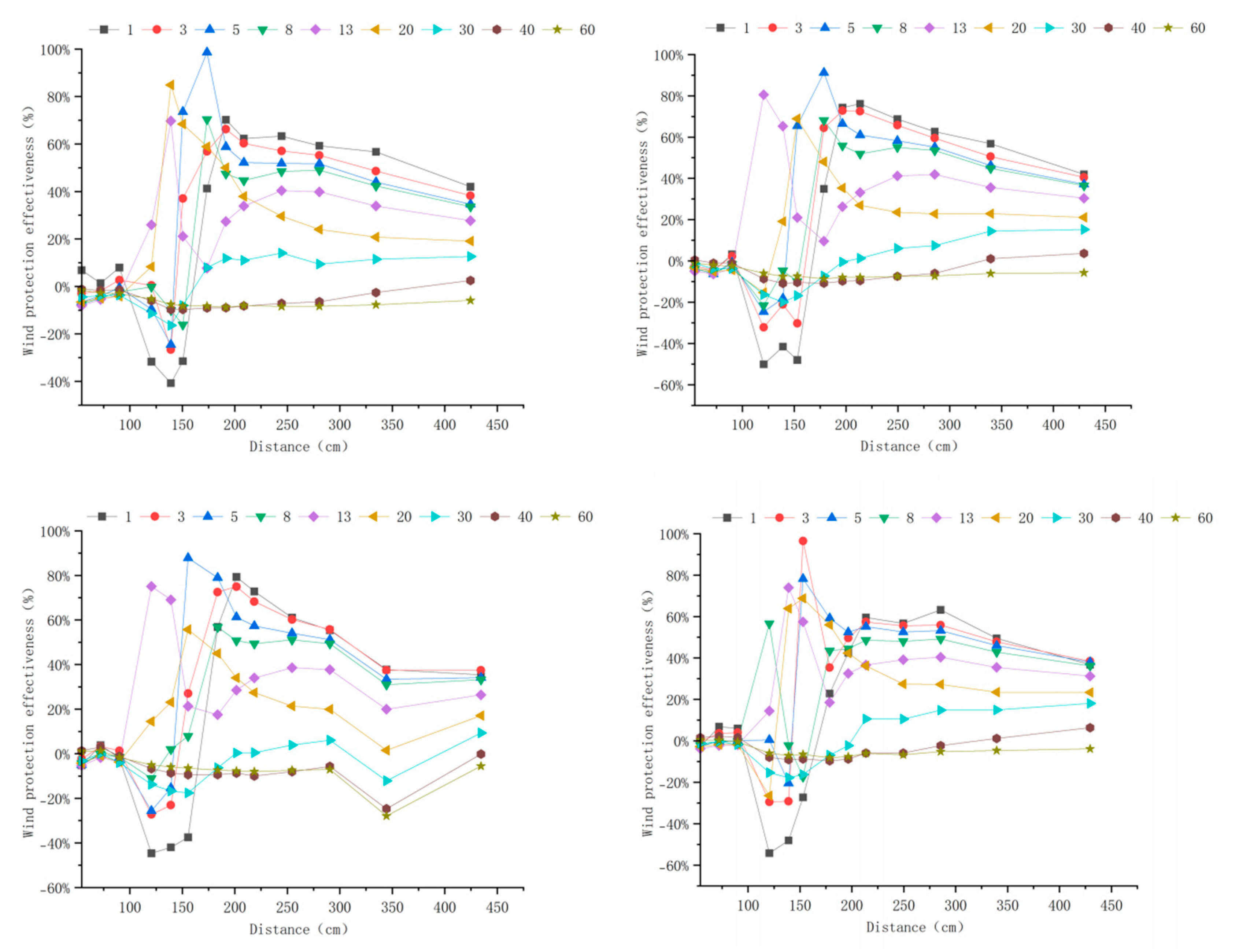
As the wind speed increased from 6 m s−1 to 10 m s−1, the windbreak efficiency at 10 m s−1 was lower than that at 6 m s−1 for all configurations. The windbreak efficiency at 10 m s−1 is illustrated in Appendix A Figure A7, Figure A8, Figure A9, Figure A10, Figure A11 and Figure A12. With the increase in wind speed, the maximum windbreak efficiency for most configurations still occurred at 7H. However, for the “P e 7.5 cm × 10 cm, T c 5 cm × 7.5 cm” combination, the peak efficiency shifted to 10H. For the “P e 7.5 cm × 10 cm, T c. 5 cm × 10 cm” configuration, the average windbreak efficiency was 20.44%, higher than that of other configurations, with the maximum windbreak efficiency at 10H reaching 40.04%. Additionally, windbreak efficiency remained relatively high (above 32%) between 1 and 15H. When the row spacing of P e was 7.5 cm × 12.5 cm, its windbreak efficiency between 1 and 15H (13.87%) was significantly higher than that of other pure P e forests. Similarly, for T c with a row spacing of 5 cm × 5 cm, its windbreak efficiency between 1 and 15H (13.82%) was significantly higher than that of other pure T c forests.
Regarding windbreak efficiency at different heights, most tree-shrub combinations reached their maximum efficiency at 1.2 times the model height (20 cm). For the “P e 7.5 cm × 7.5 cm, T c 5 cm × 5 cm” combination, the highest windbreak efficiency occurred at 20 cm, with a value of 39.45%. For pure T c forests, the maximum windbreak efficiency occurred at 3 cm, peaking at 51.96% for a row spacing of 5 cm × 5 cm. For pure P e forests, the maximum windbreak efficiency occurred at 20 cm, with a peak value of 32.31% for a row spacing of 7.5 cm × 7.5 cm.

3.3.3. Windbreak Efficiency Analysis at 15 m s−1

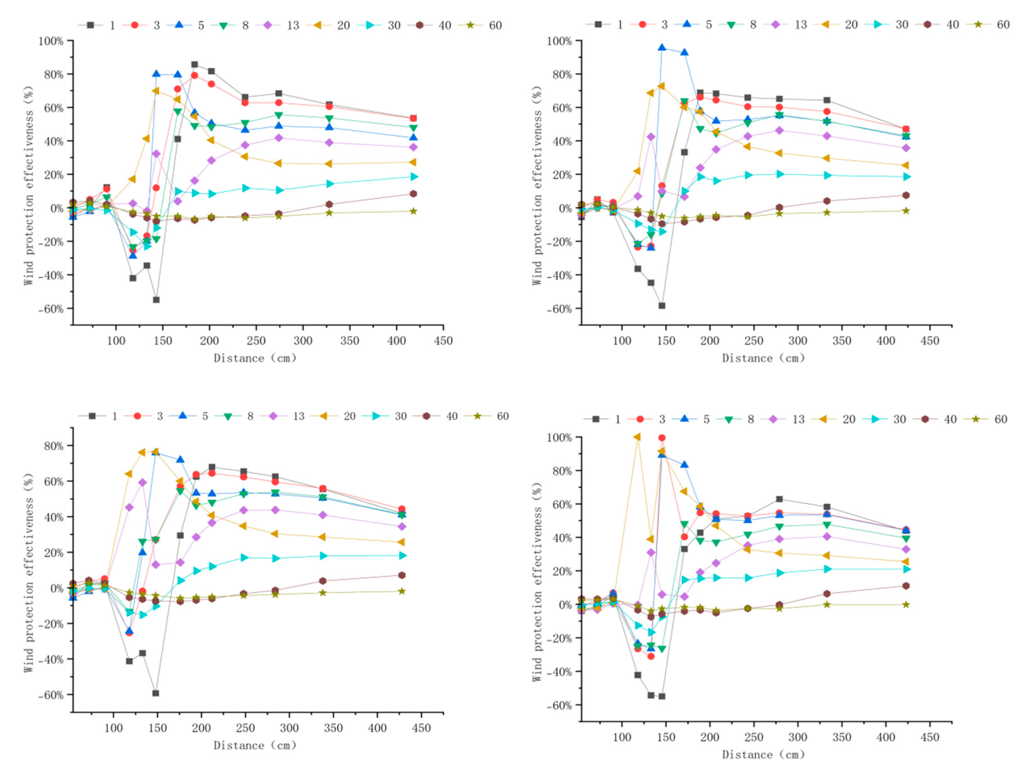
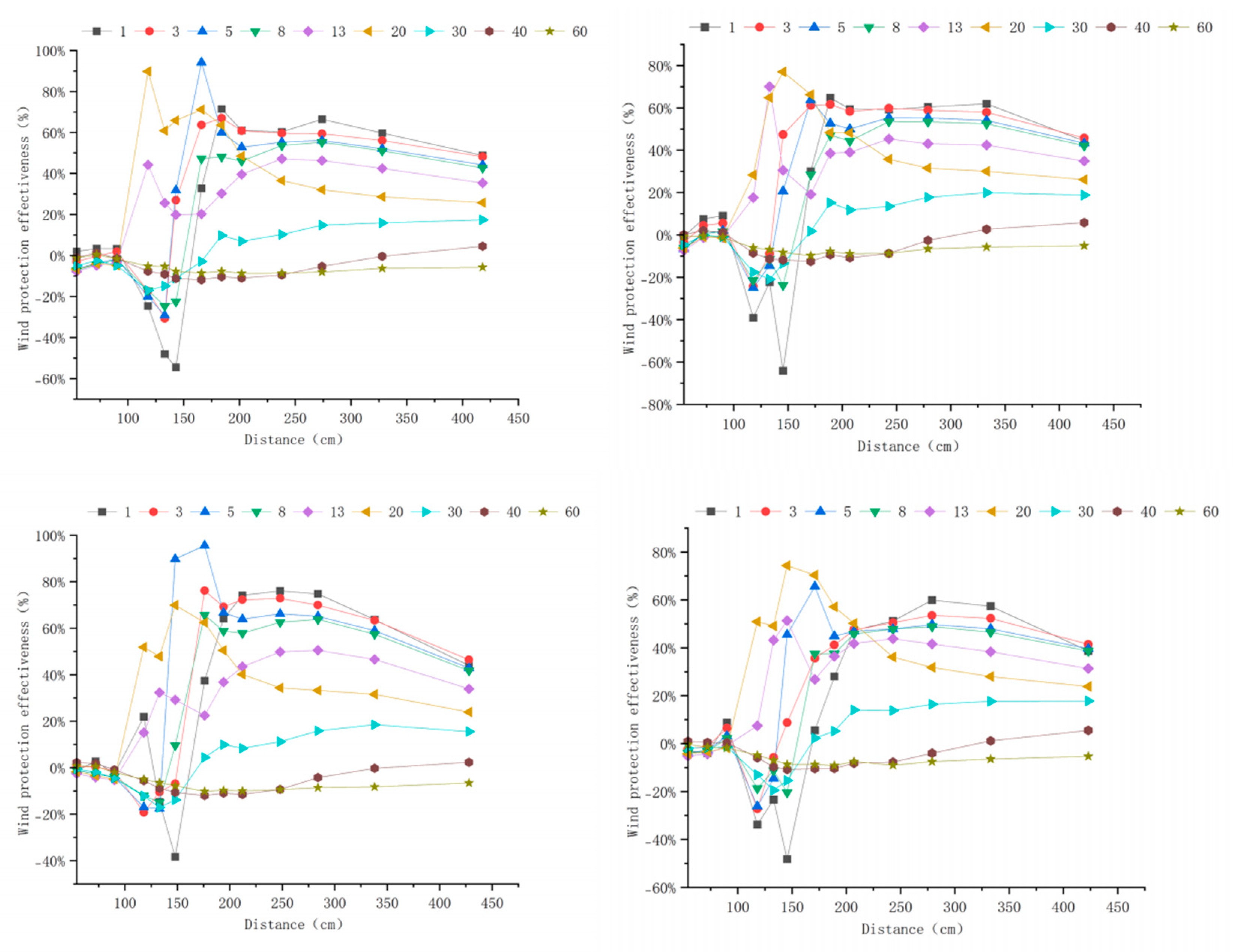
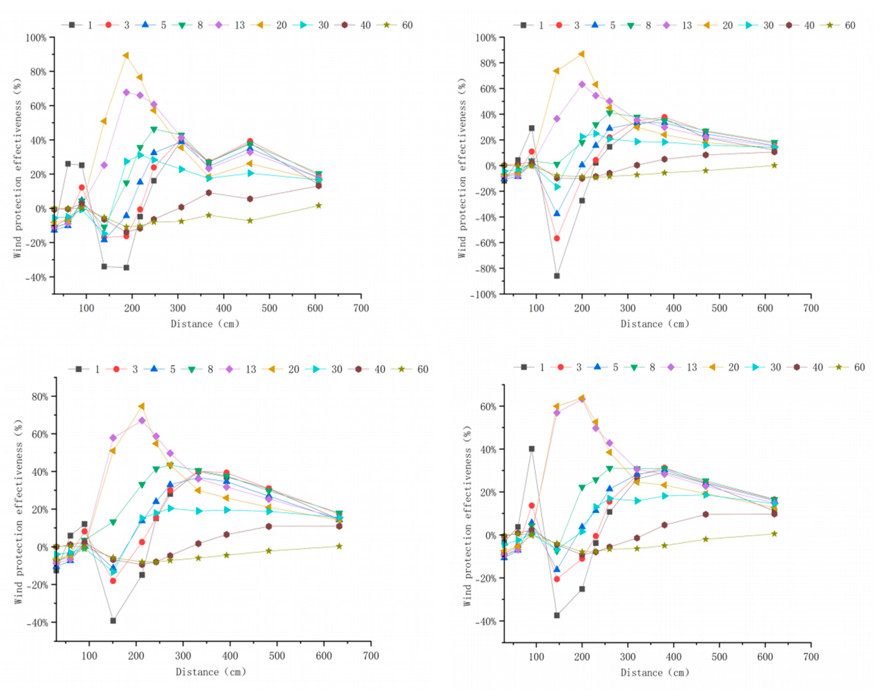
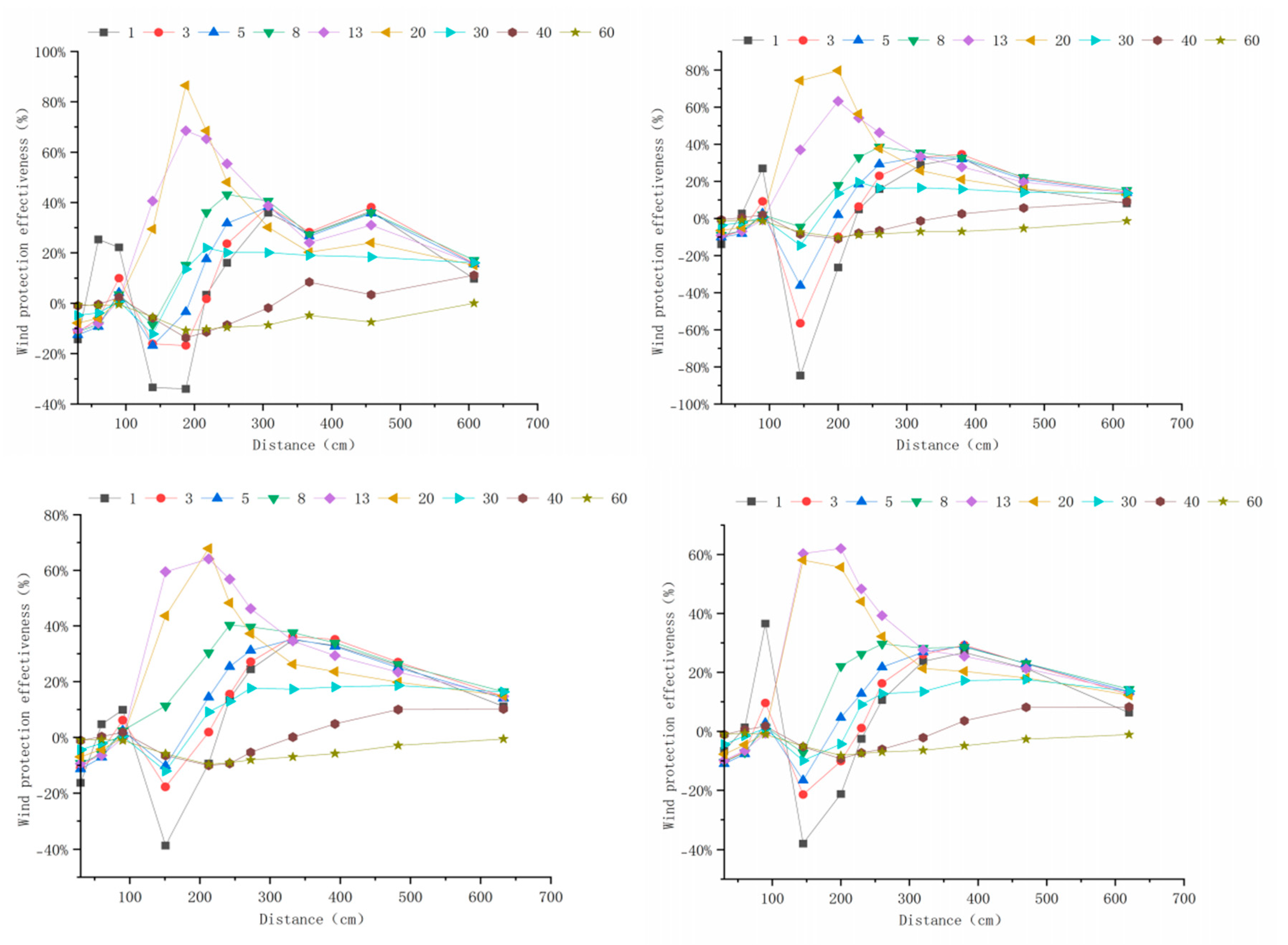
As the wind speed increased from 10 m s−1 to 15 m s−1, the windbreak efficiency of all models decreased further. The windbreak efficiency at 15 m s−1 is shown in Appendix A Figure A13, Figure A14, Figure A15, Figure A16, Figure A17 and Figure A18. Among the different configurations, the “P e 7.5 cm × 10 cm, T c 5 cm × 10 cm” combination exhibited the highest average windbreak efficiency of 18.87%, with the maximum efficiency reaching 37.79% at 7H. The windbreak efficiency remained relatively high between 1 and 15H. For the “P e 7.5 cm × 12.5 cm” configuration, the windbreak efficiency at 1–15H (12.29%) was the highest among all pure P e forests. Similarly, for the “T c 5 cm × 5 cm” configuration, the average windbreak efficiency (12.55%) was the highest among all pure T c forests.
In terms of windbreak efficiency at different heights, most tree-shrub configurations reached their maximum efficiency at 1.2 times the model height (20 cm). For the “P e 7.5 cm × 10 cm, T c 5 cm × 5 cm” combination, the maximum windbreak efficiency occurred at 20 cm, with a value of 36.72%. For pure T c forests, the maximum windbreak efficiency was observed at 3 cm, peaking at 50.23% for a row spacing of 5 cm × 10 cm. For pure P e forests, the maximum windbreak efficiency occurred at 20 cm, with a peak value of 28.31% for a row spacing of 7.5 cm × 10 cm.

4. Discussion

The present study introduces a fan-shaped, mixed-species windbreak system that combines Populus euphratica Oliv.–Tamarix chinensis Lour. Fan-shaped layouts offer distinct advantages over traditional arrangements. First, plants in fan-shaped structures utilize light more efficiently than those in conventional layouts, thereby improving the microclimate conditions for plant growth [30]. Second, the radial structure promotes airflow dispersion and energy buffering, extending protective distances and enabling shelterbelts to perform better in extreme environments such as wind erosion, dust storms, and drought [15,31,32]. Furthermore, multi-species mixed shelterbelts exhibit higher ecosystem stability and resilience through ecological complementarity among species [33]. Moreover, mixed forests exhibit greater resistance to pests and diseases, making them more sustainable than monoculture stands [34]. Thus, the combination of fan-shaped layout and multi-species mixing not only enhances ecological system resilience but also demonstrates superior protective and productive efficiency in forest management.
The wind speed profiles observed in this study generally exhibited a logarithmic relationship with height, consistent with previous wind tunnel experiments [35,36]. However, deviations such as exponential or alternative patterns have also been reported [37,38], indicating that wind profiles are strongly dependent on experimental settings. Across different tree–shrub combination models, airflow diversion created a distinct acceleration zone above the canopy [39], while near-surface zones exhibited strong deceleration due to both vegetation obstruction and surface friction. This agrees with findings on low-pressure recirculation behind forest belts [40,41,42].
A key observation was the superior performance of tree–shrub combinations compared to pure stands [43]. The vertical stratification provided by P e and T c created complementary protective layers: the tall trees dissipated upper-level flow, while the shrubs reduced near-ground turbulence, thereby extending the protection distance. This structural complementarity has been emphasized in earlier studies [44,45,46] and contrasts with pure stands, where uniformity restricts buffering capacity and accelerates efficiency decay. Similar mechanisms of “vertical complementary reduction” have been discussed by Ghisalberti & Nepf and Mukherjee further supporting the observed synergy [47,48].
Differences between this study and previous reports (peak efficiency above 90% at 5H [19]) are likely attributable to forest structure, planting layout, and wind speed conditions. The fan-shaped configuration tested here facilitated greater airflow dissipation than rectangular layouts, consistent with the argument that spatial heterogeneity enhances aerodynamic resistance [9,49]. In the vertical direction, the complementary arrangement allowed maximum efficiency to occur at approximately canopy height, with airflow disturbances shifting upward at higher wind speeds. This finding aligns with Liu [39] and Sun [11], who reported expansion of the acceleration zone with increasing velocity. However, at high wind speeds, the protective effect of all configurations declined, reaffirming the universal vulnerability of shelterbelts under extreme conditions [50,51].
Unlike previous experiments limited to pure stands or uniform rectangular layouts, it systematically evaluates mixed Populus euphratica Oliv.–Tamarix chinensis Lour. belts arranged in a novel fan-shaped configuration. By classifying airflow into deceleration, transition, and acceleration zones and testing across multiple wind speeds, the study not only quantifies the dynamic protection capacity of different structures but also proposes practical spacing guidelines tailored for arid-zone windbreak construction. Overall, the results highlight the ecological and structural advantages of mixed tree–shrub windbreaks. By combining species with contrasting canopy traits, they provide sustained efficiency and broader protection compared to pure stands. Nevertheless, the wind tunnel setting may not fully replicate natural variability, and future studies should incorporate different row numbers and spacing arrangements to optimize real-world applications.

5. Conclusions

This study highlights the advantages of fan-shaped, mixed Populus–Tamarix shelterbelts as an effective model for arid-zone restoration. The main conclusions are:
Proposes and validates a fan-shaped mixed forest belt design (Populus–Tamarix), whose wind tunnel test results demonstrate superior windbreak performance compared to single-species belts and traditional rectangular belts, highlighting the significant advantages of structural innovation.
The key to its high-efficiency protection lies in the vertical complementarity of the mixed tree-shrub system: trees reduce upper-layer wind speeds and lift airflow, while shrubs effectively lower near-surface wind speeds, forming a layered protection mechanism that significantly extends the effective distance of the protective strip.
The fan-shaped layout employs progressively widening row spacings to dissipate wind energy more gradually, avoiding the turbulence concentration commonly seen in rectangular strips. This design maintains stable protective performance even under strong winds, demonstrating superior adaptability.
Moderately dense mixed tree–shrub (P e spaced at 7.5 cm × 10 cm and T c at 5 cm × 10 cm) belts balance protective efficiency with reduced planting density, lowering resource investment costs. This design offers a practical model for shelterbelt construction and ecological restoration in arid regions, possessing significant application value.

Author Contributions

F.L.: Writing—original draft, Methodology. Q.L.: Writing—review and editing, Funding acquisition. J.Y.: Methodology, Investigation. R.C.: Methodology, Data curation. P.H., Z.W., Y.Q. and M.H.: Methodology, Investigation. All authors have read and agreed to the published version of the manuscript.

Funding

This research was funded by the National Key Research and Development Program of China (Grant No. 2023YFF130420301, Selection and Configuration Models of Superior Native Sand-fixing Plants).

Data Availability Statement

The original contributions presented in this study are included in the article. Further inquiries can be directed to the corresponding author.

Conflicts of Interest

The authors declare that they have no known competing financial interests or personal relationships that could have appeared to influence the work reported in this paper.

Nomenclature

Symbol/AbbreviationMeaningUnit
EWindbreak efficiency%
Htrees heightm
UWind speedm s−1
U0Reference (incoming) wind speedm s−1
U/U0Relative wind speed
P ePopulus euphratica Oliv.
T cTamarix chinensis Lour.

Appendix A. Windbreak Efficiency Across Configurations (6–15 m s−1)
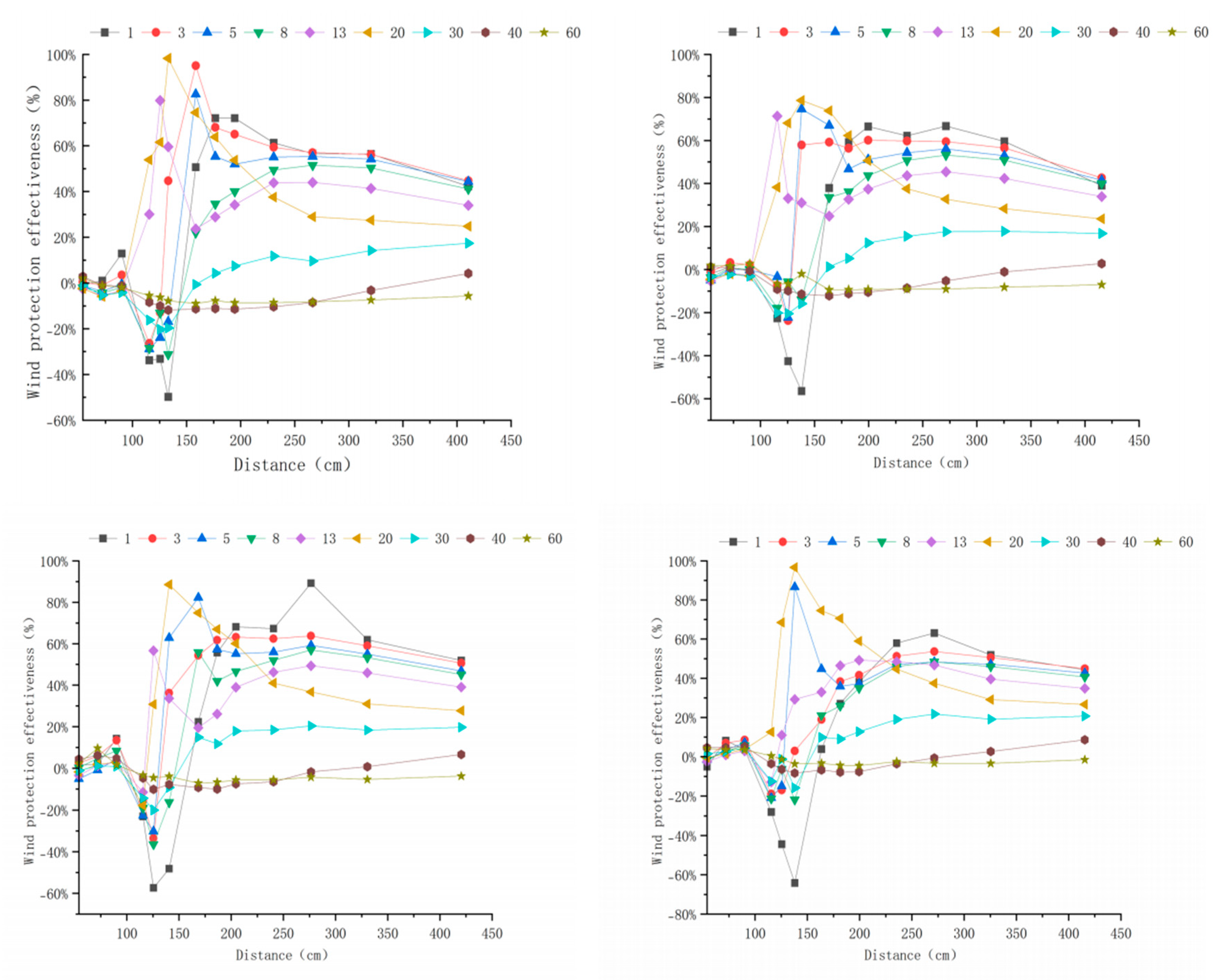
Windbreak Efficiency Diagram at 6 m s−1
Figure A1. Windbreak efficiency chart for the tree-shrub combination with P e planted at a spacing of 7.5 cm × 7.5 cm.
Forests 16 01710 g0a1
Figure A2. Windbreak efficiency chart for the tree-shrub combination with P e planted at a spacing of 7.5 cm × 10 cm.
Forests 16 01710 g0a2
Figure A3. Windbreak efficiency chart for the tree-shrub combination with P e planted at a spacing of 7.5 cm × 12.5 cm.
Forests 16 01710 g0a3
Figure A4. Windbreak efficiency chart for the tree-shrub combination with P e planted at a spacing of 10 cm × 10 cm.
Forests 16 01710 g0a4
Figure A5. Windbreak Efficiency of T c at Different Plant Spacings.
Forests 16 01710 g0a5
Figure A6. Windbreak Efficiency of P e with Different Plant Spacing.
Forests 16 01710 g0a6
Windbreak Efficiency Diagram at 10 m s−1
Figure A7. Windbreak efficiency chart for the tree-shrub combination with P e planted at a spacing of 7.5 cm × 7.5 cm.
Forests 16 01710 g0a7
Figure A8. Windbreak efficiency chart for the tree-shrub combination with P e planted at a spacing of 7.5 cm × 10 cm.
Forests 16 01710 g0a8
Figure A9. Windbreak efficiency chart for the tree-shrub combination with P e planted at a spacing of 7.5 cm × 12.5 cm.
Forests 16 01710 g0a9
Figure A10. Windbreak efficiency chart for the tree-shrub combination with P e planted at a spacing of 10 cm × 10 cm.
Forests 16 01710 g0a10
Figure A11. Windbreak Efficiency of T c at Different Plant Spacings.
Forests 16 01710 g0a11
Figure A12. Windbreak Efficiency of P e with Different Plant Spacing.
Forests 16 01710 g0a12
Windbreak Efficiency Diagram at 15 m s−1
Figure A13. Windbreak efficiency chart for the tree-shrub combination with P e planted at a spacing of 7.5 cm × 7.5 cm.
Forests 16 01710 g0a13
Figure A14. Windbreak efficiency chart for the tree-shrub combination with P e planted at a spacing of 7.5 cm × 10 cm.
Forests 16 01710 g0a14
Figure A15. Windbreak efficiency chart for the tree-shrub combination with P e planted at a spacing of 7.5 cm × 12.5 cm.
Forests 16 01710 g0a15
Figure A16. Windbreak efficiency chart for the tree-shrub combination with P e planted at a spacing of 10 cm × 10 cm.
Forests 16 01710 g0a16
Figure A17. Windbreak Efficiency of T c at Different Plant Spacing.
Forests 16 01710 g0a17
Figure A18. Windbreak Efficiency of P e at Different Plant Spacing.
Forests 16 01710 g0a18

Appendix B. Technical Details

Appendix B.1. Terminology Definition

To ensure consistency and clarity, the following terminology is adopted throughout this study. Relative wind speed (V/V0): the ratio of wind speed measured within or behind the windbreak (V) to the reference wind speed without the windbreak (V0). Based on this parameter, three zones are defined:
Deceleration Zone (0 < V/V0 ≤ 0.6): wind speed reduced by ≥40%, representing effective protection.
Transition Zone (0.6 < V/V0 ≤ 1.0): wind speed reduced but less effectively.
Acceleration Zone (V/V0 > 1.0): wind speed enhanced due to turbulence or flow contraction.
Relative Wind Speed Area Ratio (%): the proportion of the measurement area falling into the above-defined zones, used to quantify the spatial extent of wind speed reduction or acceleration.
Wind Speed Reduction (%): the percentage decrease in wind speed relative to the reference flow, calculated as (1 − V/V0) × 100%.
Windbreak Efficiency (%): the integrated indicator of the protective effect of a windbreak, calculated according to Equation (2). This term is used consistently in the manuscript instead of alternatives such as “wind protection effectiveness”.
In this study, all figures and tables employ the above terminology, and all percentages are explicitly reported with units (%).

Appendix B.2. Area Distribution Chart for Relative Wind Speed

Table A1. Relative Wind Speed Area Ratio (%) at 6 m s−1.
ModelU/U0Proportion (%)ModelU/U0Proportion (%)
T c 5 cm × 5 cm0–0.63.45T c 5 cm × 7.5 cm0–0.65.06
0.6–131.680.6–131.13
>161.78>163.81
T c 5 cm × 10 cm0–0.67.07T c 7.5 cm × 7.5 cm0–0.64.54
0.6–127.50.6–141.08
>163.81>154.38
P e 7.5 cm × 7.5 cm0–0.67.04P e 7.5 cm × 10 cm0–0.64.35
0.6–179.050.6–179.37
>113.91>116.26
P e 7.5 cm × 12.5 cm0–0.65.83P e 10 cm × 10 cm0–0.62.97
0.6–179.540.6–185.94
>114.63>111.09
P e 7.5 cm × 7.5 cm,
T c 5 cm × 5 cm
0–0.621.45P e 7.5 cm × 7.5 cm,
T c 5 cm × 7.5 cm
0–0.623.58
0.6–138.980.6–155.07
>139.57>121.35
P e 7.5 cm × 7.5 cm,
T c 5 cm × 10 cm
0–0.611.66P e 7.5 cm × 7.5 cm,
T c 7.5 cm × 7.5 cm
0–0.615.62
0.6–154.360.6–159.35
>133.9>125.03
P e 7.5 cm × 10 cm,
T c 5 cm × 5 cm
0–0.624.56P e 7.5 cm × 10 cm,
T c 5 cm × 7.5 cm
0–0.623.69
0.6–157.660.6–155.78
>117.78>120.53
P e 7.5 cm × 10 cm,
T c 5 cm × 10 cm
0–0.623.93P e 7.5 cm × 10 cm,
T c 7.5 cm × 7.5 cm
0–0.622.92
0.6–153.500.6–157.51
>122.57>119.57
P e 7.5 cm × 12.5 cm,
T c 5 cm × 5 cm
0–0.621.25P e 7.5 cm × 12.5 cm,
T c 5 cm × 7.5 cm
0–0.615.81
0.6–157.500.6–149.41
>121.25>134.78
P e 7.5 cm × 12.5 cm,
T c 5 cm × 10 cm
0–0.611.67P e 7.5 cm × 12.5 cm,
T c 7.5 cm × 7.5 cm
0–0.618.6
0.6–154.360.6–158.2
>133.97>123.2
P e 10 cm × 10 cm,
T c 5 cm × 5 cm
0–0.614.56P e 10 cm × 10 cm,
T c 5 cm × 7.5 cm
0–0.616.71
0.6–154.360.6–153.10
>131.82>130.19
P e 10 cm × 10 cm,
T c 5 cm × 10 cm
0–0.614.62P e 10 cm × 10 cm,
T c 7.5 cm × 7.5 cm
0–0.613.23
0.6–157.290.6–163.25
>128.08>123.52
Table A2. Relative Wind Speed Area Percentage at 10 m s−1 (%).
ModelU/U0Proportion (%)ModelU/U0Proportion (%)
T c 5 cm × 5 cm0–0.65.20T c 5 cm × 7.5 cm0–0.64.35
0.6–111.730.6–112.22
>183.07>183.43
T c 5 cm × 10 cm0–0.65.67T c 7.5 cm × 7.5 cm0–0.63.27
0.6–112.790.6–113.41
>181.54>183.32
P e 7.5 cm × 7.5 cm0–0.64.55P e 7.5 cm × 10 cm0–0.63.14
0.6–172.660.6–174.61
>122.79>122.25
P e 7.5 cm × 12.5 cm0–0.63.12P e 10 cm × 10 cm0–0.61.26
0.6–176.810.6–178.14
>120.07>120.6
P e 7.5 cm × 7.5 cm,
T c 5 cm × 5 cm
0–0.621.45P e 7.5 cm × 7.5 cm,
T c 5 cm × 7.5 cm
0–0.616.56
0.6–138.980.6–145.72
>139.57>137.72
P e 7.5 cm × 7.5 cm,
T c 5 cm × 10 cm
0–0.614.27P e 7.5 cm × 7.5 cm,
T c 7.5 cm × 7.5 cm
0–0.68.17
0.6–143.600.6–146.46
>142.13>145.37
P e 7.5 cm × 10 cm,
T c 5 cm × 5 cm
0–0.624.56P e 7.5 cm × 10 cm,
T c 5 cm × 7.5 cm
0–0.616.5
0.6–157.660.6–147.42
>117.78>136.08
P e 7.5 cm × 10 cm,
T c 5 cm × 10 cm
0–0.617.96P e 7.5 cm × 10 cm,
T c 7.5 cm × 7.5 cm
0–0.613.55
0.6–142.580.6–148.35
>139.46>138.1
P e 7.5 cm × 12.5 cm,
T c 5 cm × 5 cm
0–0.622.93P e 7.5 cm × 12.5 cm,
T c 5 cm × 7.5 cm
0–0.611.59
0.6–157.510.6–143.30
>119.56>145.11
P e 7.5 cm × 12.5 cm,
T c 5 cm × 10 cm
0–0.67.09P e 7.5 cm × 12.5 cm,
T c 7.5 cm × 7.5 cm
0–0.614.09
0.6–143.840.6–155.48
>149.07>130.43
P e 10 cm × 10 cm,
T c 5 cm × 5 cm
0–0.614.56P e 10 cm × 10 cm,
T c 5 cm × 7.5 cm
0–0.611.32
0.6–153.620.6–144.62
>131.83>144.06
P e 10 cm × 10 cm,
T c 5 cm × 10 cm
0–0.610.85P e 10 cm × 10 cm,
T c 7.5 cm × 7.5 cm
0–0.66.68
0.6–150.410.6–159.95
>138.74>133.37
Table A3. Relative Wind Speed Area Ratio (%) at 15 m s−1.
ModelU/U0Proportion (%)ModelU/U0Proportion (%)
T c 5 cm × 5 cm0–0.64.65T c 5 cm × 7.5 cm0–0.64.04
0.6–111.920.6–112.49
>183.43>183.47
T c 5 cm × 10 cm0–0.64.97T c 7.5 cm × 7.5 cm0–0.62.61
0.6–112.790.6–112.54
>182.22>184.85
P e 7.5 cm × 7.5 cm0–0.63.39P e 7.5 cm × 10 cm0–0.62.24
0.6–170.700.6–170.03
>125.91>127.73
P e 7.5 cm × 12.5 cm0–0.62.00P e 10 cm × 10 cm0–0.60.85
0.6–173.970.6–174.80
>124.03>124.35
P e 7.5 cm × 7.5 cm,
T c 5 cm × 5 cm
0–0.613.44P e 7.5 cm × 7.5 cm,
T c 5 cm × 7.5 cm
0–0.614.63
0.6–142.180.6–146.16
>144.38>139.21
P e 7.5 cm × 7.5 cm,
T c 5 cm × 10 cm
0–0.612.30P e 7.5 cm × 7.5 cm,
T c 7.5 cm × 7.5 cm
0–0.66.23
0.6–144.420.6–147.22
>143.28>146.55
P e 7.5 cm × 10 cm,
T c 5 cm × 5 cm
0–0.614.55P e 7.5 cm × 10 cm,
T c 5 cm × 7.5 cm
0–0.612.86
0.6–143.510.6–148.97
>141.94>138.17
P e 7.5 cm × 10 cm,
T c 5 cm × 10 cm
0–0.615.07P e 7.5 cm × 10 cm,
T c 7.5 cm × 7.5 cm
0–0.611.05
0.6–140.820.6–149.31
>144.11>139.64
P e 7.5 cm × 12.5 cm,
T c 5 cm × 5 cm
0–0.610.90P e 7.5 cm × 12.5 cm,
T c 5 cm × 7.5 cm
0–0.610.32
0.6–143.850.6–143.37
>145.25>146.31
P e 7.5 cm × 12.5 cm,
T c 5 cm × 10 cm
0–0.66.85P e 7.5 cm × 12.5 cm,
T c 7.5 cm × 7.5 cm
0–0.610.09
0.6–141.000.6–152.68
>152.15>137.23
P e 10 cm × 10 cm,
T c 5 cm × 5 cm
0–0.69.26P e 10 cm × 10 cm,
T c 5 cm × 7.5 cm
0–0.610.16
0.6–145.520.6–145.20
>145.22>144.64
P e 10 cm × 10 cm,
T c 5 cm × 10 cm
0–0.611.08P e 10 cm × 10 cm,
T c 7.5 cm × 7.5 cm
0–0.64.79
0.6–150.230.6–154.17
>138.69>141.04

References

  1. Durán Zuazo, V.H.; Rodríguez Pleguezuelo, C.R. Soil-erosion and runoff prevention by plant covers. A review. Agron. Sustain. Dev. 2008, 28, 65–86. [Google Scholar] [CrossRef]
  2. Gadiga, B.L.; Dan, Y. Evaluating the Role of Shelterbelt in Vegetation Development in a Semi Arid Zone of Yobe State, Nigeria. J. Geogr. Inf. Syst. 2015, 7, 541–550. [Google Scholar] [CrossRef]
  3. Zhan, K.; Liu, S.; Yang, Z.; Fang, E.; Zhou, L.; Huang, N. Effects of sand-fixing and windbreak forests on wind flow: A synthesis of results from field experiments and numerical simulations. J. Arid Land 2017, 9, 1–12. [Google Scholar] [CrossRef]
  4. Jones, R.E.; Vere, D.T.; Campbell, M.H. The external costs of pasture weed spread: An economic assessment of serrated tussock control. Agric. Econ. 2000, 22, 91–103. [Google Scholar] [CrossRef]
  5. Boldes, U.; Golberg, A.; Di Leo, J.M.; Colman, J.; Scarabino, A. Canopy flow and aspects of the response of plants protected by herbaceous shelterbelts and wood fences. J. Wind Eng. Ind. Aerodyn. 2002, 90, 1253–1270. [Google Scholar] [CrossRef]
  6. Cleugh, H.A. Effects of windbreaks on airflow, microclimates and crop yields. Agrofor. Syst. 1998, 41, 55–84. [Google Scholar] [CrossRef]
  7. Torita, H.; Satou, H. Relationship between shelterbelt structure and mean wind reduction. Agric. For. Meteorol. 2007, 145, 186–194. [Google Scholar] [CrossRef]
  8. Raine, J.K.; Stevenson, D.C. Wind protection by model fences in a simulated atmospheric boundary layer. J. Wind Eng. Ind. Aerodyn. 1977, 2, 159–180. [Google Scholar] [CrossRef]
  9. Bitog, J.P.; Lee, I.-B.; Hwang, H.-S.; Shin, M.-H.; Hong, S.-W.; Seo, I.-H.; Kwon, K.-S.; Mostafa, E.; Pang, Z. Numerical simulation study of a trees windbreak. Biosyst. Eng. 2012, 111, 40–48. [Google Scholar] [CrossRef]
  10. Heisler, G.M.; Dewalle, D.R. Effects of windbreak structure on wind flow. Agric. Ecosyst. Environ. 1988, 22–23, 41–69. [Google Scholar] [CrossRef]
  11. Sun, Q.; Zheng, B.; Liu, T.; Zhu, L.; Hao, X.; Han, Z. The optimal spacing interval between principal shelterbelts of the farm-shelter forest network. Environ. Sci. Pollut. Res. 2022, 29, 12680–12693. [Google Scholar] [CrossRef] [PubMed]
  12. Cai, X.; Henderson, M.; Wang, L.; Su, Y.; Liu, B. Shelterbelt Structure and Crop Protection from Increased Typhoon Activity in Northeast China. Agriculture 2021, 11, 995. [Google Scholar] [CrossRef]
  13. Pretzsch, H.; Del Río, M.; Schütze, G.; Ammer, C.; Annighöfer, P.; Avdagic, A.; Barbeito, I.; Bielak, K.; Brazaitis, G.; Coll, L.; et al. Mixing of Scots pine (Pinus sylvestris L.) and European beech (Fagus sylvatica L.) enhances structural heterogeneity, and the effect increases with water availability. For. Ecol. Manag. 2016, 373, 149–166. [Google Scholar] [CrossRef]
  14. Frank, C.; Ruck, B. Double-Arranged Mound-Mounted Shelterbelts: Influence of Porosity on Wind Reduction between the Shelters. Environ. Fluid Mech. 2005, 5, 267–292. [Google Scholar] [CrossRef]
  15. Li, H.; Wang, Y.; Li, S.; Askar, A.; Wang, H. Shelter Efficiency of Various Shelterbelt Configurations: A Wind Tunnel Study. Atmosphere 2022, 13, 1022. [Google Scholar] [CrossRef]
  16. Balakin, V.V. Formation of linear-strip greening objects in urban environmental systems. IOP Conf. Ser. Mater. Sci. Eng. 2018, 451, 012166. [Google Scholar] [CrossRef]
  17. Guyot, G. Brise-vent, pare-feu et sylviculture. Rev. For. Française 1990, 42, 93. [Google Scholar] [CrossRef]
  18. Wilson, J.D. Numerical studies of flow through a windbreak. J. Wind Eng. Ind. Aerodyn. 1985, 21, 119–154. [Google Scholar] [CrossRef]
  19. Zhang, K.; Qu, J.; Zhang, X.; Zhao, L.; Li, S. Protective Efficiency of Railway Arbor-Shrub Windbreak Forest Belts in Gobi Regions: Numerical Simulation and Wind Tunnel Tests. Front. Environ. Sci. 2022, 10, 885070. [Google Scholar] [CrossRef]
  20. Chen, C.; Chen, J. Remote sensing analysis on the regional differentiation of land types in the Loess Plateau of the North Shaanxi Province. Natl. Remote Sens. Bull. 1992, 1, 1–8. [Google Scholar] [CrossRef]
  21. Zhang, S.; Yuan, W.; Yu, Y.; Zhang, Y.; Wang, W.; Wang, L.; Yang, Y.; Wang, H. Shrubs plays an important role in configuration of shelterbelt in windy and sandy areas. Front. Ecol. Evol. 2024, 12, 1347714. [Google Scholar] [CrossRef]
  22. Judd, M.J.; Raupach, M.R.; Finnigan, J.J. A wind tunnel study of turbulent flow around single and multiple windbreaks, part I: Velocity fields. Bound.-Layer Meteorol. 1996, 80, 127–165. [Google Scholar] [CrossRef]
  23. Mayaud, J.; Webb, N. Vegetation in Drylands: Effects on Wind Flow and Aeolian Sediment Transport. Land 2017, 6, 64. [Google Scholar] [CrossRef]
  24. Raupach, M.R.; Finnigan, J.J.; Brunet, Y. Coherent eddies and turbulence in vegetation canopies: The mixing-layer analogy. Bound.-Layer Meteorol. 1996, 78, 351–382. [Google Scholar] [CrossRef]
  25. Mayaud, J.R.; Wiggs, G.F.S.; Bailey, R.M. Characterizing turbulent wind flow around dryland vegetation. Earth Surf. Process. Landf. 2016, 41, 1421–1436. [Google Scholar] [CrossRef]
  26. Nepf, H.M.; Vivoni, E.R. Flow structure in depth–limited, vegetated flow. J. Geophys. Res. Ocean. 2000, 105, 28547–28557. [Google Scholar] [CrossRef]
  27. Horne, W.J. Flow Around a Solitary Trees in a Large Field Under Neutral Atmospheric Stratification. Ph.D. Thesis, University of Utah, Salt Lake City, UT, USA, 2012. [Google Scholar]
  28. Brandle, J.R.; Hodges, L.; Zhou, X.H. Windbreaks in North American agricultural systems. Agrofor. Syst. 2004, 61, 65–78. [Google Scholar] [CrossRef]
  29. Wang, H.; Zhang, C.; Jiang, H. Wind tunnel experiments on airflow patterns and wind erosion behind different windbreak structures. Aeolian Res. 2018, 31, 79–87. [Google Scholar] [CrossRef]
  30. Tustin, D.S.; Van Hooijdonk, B.M.; Breen, K.C. The Planar Cordon—New planting systems concepts to improve light utilisation and physiological function to increase apple orchard yield potential. Acta Hortic. 2018, 1228, 1–12. [Google Scholar] [CrossRef]
  31. Kegley, N.F. Toward the Preservation of Rural Cultural Historic Landscapes: Amethod for Evaluating Nineteenth Century Blue Ridge Farms. Master’s Thesis, Virginia Polytechnic Institute State University, Blacksburg, VA, USA, 1986. Available online: https://vtechworks.lib.vt.edu/bitstreams/7b8571e3-eccd-4946-859c-4cd1524486ab/download (accessed on 1 October 2025).
  32. Zhang, H.; Pei, L.; Li, J.; Wang, F. Numerical simulation of wind and sand resistance in three typical shrubs. Sustainability 2025, 17, 5481. [Google Scholar] [CrossRef]
  33. Messier, C.; Bauhus, J.; Doyon, F.; Maure, F.; Sousa-Silva, R.; Nolet, P.; Puettmann, K. The functional complex network approach to foster forest resilience to global changes. For. Ecosyst. 2019, 6, 21. [Google Scholar] [CrossRef]
  34. MacLean, D.A.; Clark, K.L. Mixedwood management positively affects forest health during insect infestations in eastern North America. Can. J. For. Res. 2021, 51, 910–920. [Google Scholar] [CrossRef]
  35. Singh, J.; Roy, A.K. CFD simulation of the wind field around pyramidal roofed single-story buildings. SN Appl. Sci. 2019, 1, 1425. [Google Scholar] [CrossRef]
  36. Zhang, Y.; Wang, Y.H.W. Analysis of creeping sand trajectories using high-speed photography. Chin. Sci. Bull. 2010, 55, 3186–3192. [Google Scholar] [CrossRef]
  37. Sankaran, A.; Hain, R.; Kähler, C. Assessing the dispersion characteristics of ship exhausts in neutral boundary layers: Wind tunnel testing. In PHYSMOD 2024, Proceedings of the International Workshop on Physical Modelling of Flow and Dispersion Phenomena, Lyon, France, 28–30 August 2024; HAL Open Science: Lyon, France, 2024; pp. 118–126. [Google Scholar]
  38. Cui, K.; Li, S.; Wang, H.; Fan, J. Three dimensional flow field characteristics of two typical blowouts in the dry lake basin of Taitema Lake and their influence on wind erosion. Arid Land. Geogr. 2022, 45, 1784–1794. [Google Scholar] [CrossRef]
  39. Ma, R.; Wang, J.; Qu, J.; Liu, H. Effectiveness of shelterbelt with a non-uniform density distribution. J. Wind Eng. Ind. Aerodyn. 2010, 98, 767–771. [Google Scholar] [CrossRef]
  40. Lampartová, I.; Schneider, J.; Vyskot, I.; Rajnoch, M.; Litschmann, T. Impact of protective shelterbelt microclimate characteristics. Ekológia 2015, 34, 101–110. [Google Scholar] [CrossRef]
  41. Dong, Z.; Luo, W.; Qian, G.; Wang, H. Experimental investigation of the sheltering effect of porous fences on sand flux profiles. Geomorphology 2018, 310, 74–83. [Google Scholar] [CrossRef]
  42. Cheng, H.; He, W.; Liu, C.; Zou, X.; Kang, L.; Chen, T.; Zhang, K. Transition model for airflow fields from single plants to multiple plants. Agric. For. Meteorol. 2019, 266–267, 29–42. [Google Scholar] [CrossRef]
  43. Li, J.; Dong, S.; Li, Y. Comparative study on windbreak effects of two different configuration shelterbelts. IOP Conf. Ser. Earth Environ. Sci. 2021, 895, 012020. [Google Scholar] [CrossRef]
  44. Kainkwa, R.M.R.; Stigter, C.J. Wind reduction downwind from a savanna woodland edge. Neth. J. Agric. Sci. 1994, 42, 145–157. [Google Scholar] [CrossRef]
  45. Liu, B.; Zhou, X.; Brandle, J. Effects of multiple-row trees–shrub shelterbelts on wind speed reduction and crop yield improvement in arid regions. Agrofor. Syst. 2019, 93, 541–554. [Google Scholar] [CrossRef]
  46. Leenders, J.K.; Boxel, J.H.V.; Sterk, G. The effect of single vegetation elements on wind speed and sediment transport in the Sahelian zone of Burkina Faso. Earth Surf. Process. Landf. 2007, 32, 1454–1474. [Google Scholar] [CrossRef]
  47. Ghisalberti, M.; Nepf, H. The Structure of the Shear Layer in Flows over Rigid and Flexible Canopies. Environ. Fluid Mech. 2006, 6, 277–301. [Google Scholar] [CrossRef]
  48. Mukherjee, A.; Cajas, J.C.; Houzeaux, G.; Lehmkuhl, O.; Suckale, J.; Marras, S. Forest density is more effective than trees rigidity at reducing the onshore energy flux of tsunamis. Coast. Eng. 2023, 182, 104286. [Google Scholar] [CrossRef]
  49. Lup, A.; Miron, L. Fighting Against Drought in Dobrogea by Protective Forest Belts. Munich Personal RePEc Archive (MPRA), No. 61724, Ovidius University of Constanta. 20 November 2014. Available online: https://mpra.ub.uni-muenchen.de/61724 (accessed on 1 October 2025).
  50. Foster, D.R.; Boose, E.R. Patterns of Forest Damage Resulting from Catastrophic Wind in Central New England, USA. J. Eco. 1992, 80, 79–98. [Google Scholar] [CrossRef]
  51. Finnigan, J. Turbulence in plant canopies. Ann. Rev. Fluid Mech. 2000, 32, 519–791. [Google Scholar] [CrossRef]
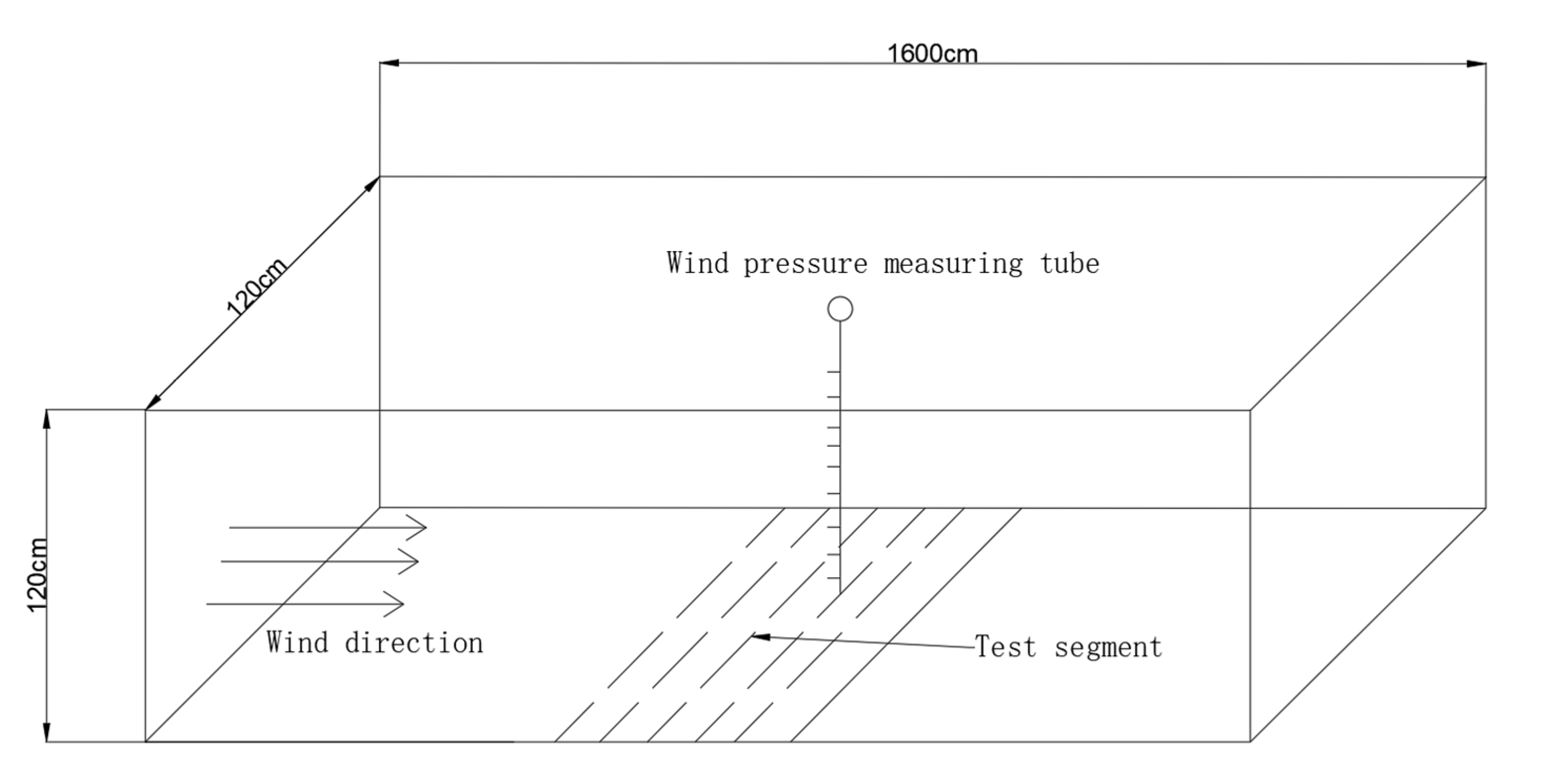
Figure 1. Schematic layout of the wind tunnel model.
Forests 16 01710 g001
Figure 2. Models of the Plants and Configuration Diagram Used.
Forests 16 01710 g002
Figure 3. Layout of arbor (Populus euphratica Oliv.) and shrub (Tamarix chinensis Lour.) belts with reference to wind direction. Distances are expressed in multiples of tree height (H). Key markers indicate positions for wind speed measurement.
Forests 16 01710 g003
Figure 4. Contour plot of relative wind speed for different tree-shrub combinations at 6 m s−1 At 6 m s−1, (a) represents the combination of P e at 7.5 cm × 7.5 cm and T c. at 5 cm × 5 cm, 5 cm × 7.5 cm, 5 cm × 10 cm, and 7.5 cm × 7.5 cm; (b) represents the combination of P e at 7.5 cm × 10 cm and T c. at 5 cm × 5 cm, 5 cm × 7.5 cm, 5 cm × 10 cm, and 7.5 cm × 7.5 cm; (c) represents the combination of P e at 7.5 cm × 12.5 cm and T c at 5 cm × 5 cm, 5 cm × 7.5 cm, 5 cm × 10 cm, and 7.5 cm × 7.5 cm; (d) represents the combination of P e at 10 cm × 10 cm and T c at 5 cm × 5 cm, 5 cm × 7.5 cm, 5 cm × 10 cm, and 7.5 cm × 7.5 cm. The black line indicates the edge of the forest strip.
Forests 16 01710 g004
Figure 5. Contour map of relative wind speed for pure forests with different configurations at 6 m s−1. At 6 m s−1, on the left side, the configurations from top to bottom are T c with spacings of 5 cm × 5 cm, 5 cm × 7.5 cm, 5 cm × 10 cm, and 7.5 cm × 7.5 cm. On the right side, the configurations from top to bottom are P e with spacings of 7.5 cm × 7.5 cm, 7.5 cm × 10 cm, 7.5 cm × 12.5 cm, and 10 cm × 10 cm. The black line indicates the edge of the forest strip.
Forests 16 01710 g005
Figure 6. Contour plot of relative wind speed for different tree-shrub combinations at 10 m s−1 At 10 m s−1, (a) represents the combination of P e at 7.5 cm × 7.5 cm and T c. at 5 cm × 5 cm, 5 cm × 7.5 cm, 5 cm × 10 cm, and 7.5 cm × 7.5 cm; (b) represents the combination of P e at 7.5 cm × 10 cm and T c. at 5 cm × 5 cm, 5 cm × 7.5 cm, 5 cm × 10 cm, and 7.5 cm × 7.5 cm; (c) represents the combination of P e at 7.5 cm × 12.5 cm and T c at 5 cm × 5 cm, 5 cm × 7.5 cm, 5 cm × 10 cm, and 7.5 cm × 7.5 cm; (d) represents the combination of P e at 10 cm × 10 cm and T c at 5 cm × 5 cm, 5 cm × 7.5 cm, 5 cm × 10 cm, and 7.5 cm × 7.5 cm. The black line indicates the edge of the forest strip.
Forests 16 01710 g006
Figure 7. Contour map of relative wind speed for pure forests with different configurations at 10 m s−1. At 10 m s−1, on the left side, the configurations from top to bottom are T c with spacings of 5 cm × 5 cm, 5 cm × 7.5 cm, 5 cm × 10 cm, and 7.5 cm × 7.5 cm. On the right side, the configurations from top to bottom are P e with spacings of 7.5 cm × 7.5 cm, 7.5 cm × 10 cm, 7.5 cm × 12.5 cm, and 10 cm × 10 cm. The black line indicates the edge of the forest strip.
Forests 16 01710 g007
Figure 8. Contour plot of relative wind speed for different tree-shrub combinations at 15 m s−1 At 15 m s−1, (a) represents the combination of P e at 7.5 cm × 7.5 cm and T c at 5 cm × 5 cm, 5 cm × 7.5 cm, 5 cm × 10 cm, and 7.5 cm × 7.5 cm; (b) represents the combination of P e at 7.5 cm × 10 cm and T c at 5 cm × 5 cm, 5 cm × 7.5 cm, 5 cm × 10 cm, and 7.5 cm × 7.5 cm; (c) represents the combination of P e at 7.5 cm × 12.5 cm and T c at 5 cm × 5 cm, 5 cm × 7.5 cm, 5 cm × 10 cm, and 7.5 cm × 7.5 cm; (d) represents the combination of P e at 10 cm × 10 cm and T c at 5 cm × 5 cm, 5 cm × 7.5 cm, 5 cm × 10 cm, and 7.5 cm × 7.5 cm. The black line indicates the edge of the forest strip.
Forests 16 01710 g008
Figure 9. Contour map of relative wind speed for pure forests with different configurations at 15 m s−1. At 15 m s−1, on the left side, the configurations from top to bottom are T c with spacings of 5 cm × 5 cm, 5 cm × 7.5 cm, 5 cm × 10 cm, and 7.5 cm × 7.5 cm. On the right side, the configurations from top to bottom are P e with spacings of 7.5 cm × 7.5 cm, 7.5 cm × 10 cm, 7.5 cm × 12.5 cm, and 10 cm × 10 cm. The black line indicates the edge of the forest strip.
Forests 16 01710 g009
Table 1. Model Plant Spacing and Belt Width.
P e Plant SpacingT c Plant Row SpacingBelt Width (cm)
7.5 cm × 7.5 cm5 cm × 5 cm40.5
5 cm × 7.5 cm45.5
5 cm × 10 cm50.5
7.5 cm × 7.5 cm45.5
7.5 cm × 10 cm5 cm × 5 cm48
5 cm × 7.5 cm53
5 cm × 10 cm58
7.5 cm × 7.5 cm53
7.5 cm × 12.5 cm5 cm × 5 cm55.5
5 cm × 7.5 cm60.5
5 cm × 10 cm65.5
7.5 cm × 7.5 cm60.5
10 cm × 10 cm5 cm × 5 cm48
5 cm × 7.5 cm53
5 cm × 10 cm58
7.5 cm × 7.5 cm53
Table 2. Initial wind speed and wind speed profile equations without the model.
Height (cm)
Speed
(m s−1)
61015
14.146.899.88
35.058.1811.68
55.428.7212.46
85.679.0812.95
136.059.6113.69
206.4010.3614.83
307.0511.1115.87
408.1112.7518.06
608.9113.8919.50
Wind Speed Profile Equationu = 1.07928769ln(z) + 3.72818485
R2 = 0.91
u = 1.5986ln(z) + 6.2403
R2 = 0.91
u = 2.53ln(z) + 8.06
R2 = 0.91
Disclaimer/Publisher’s Note: The statements, opinions and data contained in all publications are solely those of the individual author(s) and contributor(s) and not of MDPI and/or the editor(s). MDPI and/or the editor(s) disclaim responsibility for any injury to people or property resulting from any ideas, methods, instructions or products referred to in the content.