Article

Parameter Optimization for Robust Urban Tree Crown Delineation: Enhancing Accuracy in Raster-Based Segmentation

by
Nikita A. Isaykin
1,
Nataly I. Zaznobina
1 and
Basil N. Yakimov
1,2,*,†
1
Department of Ecology, Institute of Biology and Biomedicine, Lobachevsky State University of Nizhny Novgorod, Gagarin Avenue 23, 603022 Nizhny Novgorod, Russia
2
Faculty of Biology, Shenzhen MSU-BIT University, Shenzhen 518172, China
*
Author to whom correspondence should be addressed.
MSU-BIT University is author’s primary affiliation.
Forests 2025, 16(11), 1655; https://doi.org/10.3390/f16111655 (registering DOI)
Submission received: 23 September 2025 / Revised: 24 October 2025 / Accepted: 28 October 2025 / Published: 30 October 2025

Abstract

Accurate and efficient delineation of individual tree crowns is crucial for urban forest inventories and ecosystem service assessments but is often limited by the manual selection of parameters for segmentation algorithms. This study investigates the impact of parameter optimization on the performance of four common raster-based segmentation algorithms—Watershed, Marker-Controlled Watershed, Dalponte, and Silva—for individual tree crown detection. Utilizing UAV-derived Canopy Height Models from the Lobachevsky University campus, we employed Random Search and Differential Evolution methods to systematically optimize algorithm parameters. Our findings reveal that relying on default or field-data-derived parameters significantly constrains segmentation accuracy. Parameter optimization led to substantial performance improvements across all algorithms. Notably, after optimization, the final performance (F-score values) for all algorithms converged to within a narrow range of 0.3, demonstrating that optimized simpler algorithms can achieve comparable performance to more complex ones. This research underscores that the key to accurate tree crown detection lies not solely in the choice of the segmentation method but critically in its preliminary tuning and optimization. The proposed optimization approaches enhance the accuracy and objectivity of urban tree crown delineation, providing a robust framework for improving urban forest inventories and enabling more effective application of remote sensing techniques in assessing urban ecosystem services.

1. Introduction

Urban vegetation is a vital component of the urban environment, providing a broad spectrum of ecosystem services that directly and indirectly impact human health and well-being [1,2,3]. Trees and shrubs form the basis of urban forests, constituting a significant portion of urban vegetation with a substantial influence on urban populations [4,5,6]. Urban forests contribute to physical and mental health [7], regulate the urban microclimate [8], enhance water and air quality while mitigating their pollution [9], reduce noise [10], provide aesthetic benefits, and support biodiversity conservation [11,12]. The rapid acquisition of up-to-date information on urban vegetation, including the number of trees and their condition, enables timely decision-making in urban planning and management. This underscores the importance of green spaces and urban greening initiatives, which, for instance, contribute to climate change adaptation through carbon sequestration and oxygen production [13,14,15].
Currently, two principal methodologies are utilized to gather vegetation information pertinent to the assessment of ecosystem services: direct field measurements and remote sensing. Traditionally, field inventories have been the most accurate method for collecting tree-related data, encompassing attributes such as species affiliation, trunk diameter, crown proportions, and dieback, when compared to airborne and satellite remote sensing techniques. However, this approach faces several limitations, including high time and labor costs, a restricted survey area, and potential disturbance to the objects under study [16,17,18].
The limitations of traditional methods are overcome by using active and passive remote sensing techniques [19,20], which enable the rapid collection of extensive data over large areas without direct contact with the objects of study [21,22]. Satellite data is increasingly informative and accessible; however, sub-meter resolution is typically available only for specific regions and often entails a high monetary cost [23,24]. For most areas, the spatial resolution of free-access satellite sensors, such as Landsat 7 and 8 or Sentinel 2, only permits a general estimation of vegetation cover [25,26]. Aerial imaging offers a distinct approach, providing centimeter-resolution images within study areas, thus enabling the study of individual trees, albeit with operational challenges and limited area coverage compared to satellite imagery [27,28]. Additionally, active aerial sensing methods like Light Detection and Ranging (LiDAR) provide precise and detailed three-dimensional information in the form of point clouds on the structure and spatial arrangement of studied objects [29,30]. For instance, LiDAR is effective for tree detection and digital modelling [31], facilitating automatic measurement of forest traits [22]. However, this method also presents difficulties related to the three-dimensional representation of data [32] and the interpretation of spectral features within the study area [33].
Unmanned Aerial Vehicles (UAVs) equipped with sensors represent cutting-edge, practical, and adaptable instruments for remote vegetation data gathering [27]. A more conventional application of UAVs in tree stand studies [20] involves using passive systems to collect the range of spectral information reflected from the surface of objects under study, such as optical imaging in the visible spectrum [34,35,36,37], multispectral [38,39], and hyperspectral imaging [40,41]. Photogrammetric processing of the acquired images enables the reconstruction of digital models of the topographic surface and tree canopy. The obtained spectral characteristics can be used, for example, in calculating various spectral indices [38,39,41] or for tree species classification [35,40]. Concurrently, active remote sensing technologies like LiDAR are becoming more accessible. LiDAR can be employed for more accurate reconstruction of both terrain features and the spatial structure of stands [10], which can subsequently be used to delineate tree stands or detect individual trees [42,43], or applied to different analyses and classifications [44,45]. Given that both approaches have their drawbacks, numerous studies utilize these techniques synergistically [18,24,46,47].
Simultaneously, techniques for object detection and semantic segmentation of urban areas, with a focus on green spaces using remote sensing data such as aerial imagery, are developing rapidly [5,48]. Consequently, urban forests, and in more detailed works, individual trees are becoming the focus of such research [49,50,51]. Methods for the remote estimation of the main spectral and structural parameters of individual trees are thus developed. These methods can be used, for instance, both in the detection of damaged and diseased trees [41,52,53] and for the calculation of ecosystem services [25,54]. At the same time, UAVs are increasing in popularity for agricultural purposes, forest management, and landscape ecology due to their flexibility and the capabilities of using various instruments as payload for image capture and translation [48,55,56].
Regardless of the data acquisition method, a solution for identifying individual trees and their crowns is necessary, serving as either the initial analytical step or the primary objective [57,58]. Recently, computer vision methods have advanced significantly, enabling more efficient detection of various objects, including trees [59,60,61]. For tree crown detection, sophisticated machine learning models employing Convolutional Neural Networks with instance segmentation [59,62,63] are frequently utilized. The ongoing demand for improving and examining the raster-based methods also stems from the preference of many researchers to work with raster data, specifically Canopy Height Models (CHM), when studying tree stands [20,63,64]. Consequently, region growing and watershed segmentation algorithms are the most common raster-based techniques for image segmentation in this context [18,52], with the Silva et al. [65] algorithm also being frequently used for segmenting CHMs [43,44,45,47].
All acknowledged segmentation techniques used to delimit tree crowns, regardless of the type of raw data (raster-based or point cloud-based), require user intervention at the stage of selecting input parameter values [65,66] due to the existence of a massive amount of specific cases for these algorithms: individual tree/plot-level studies, coniferous/broadleaf/mixed wood types, forest/urban areas, remote sensing data type, etc. [10,18,39,43,45,52,63]. In other words, each application case needs almost unique fine-tuning of parameter values to maximize the applied algorithm’s effectiveness.
The common workflow involves selecting a working configuration of parameters through a combination of defaults and adjustments based on ground-truth data, often with manual tuning [10,45,46,52,67]. However, the problem of selecting the optimal parameter configuration remains unresolved and requires deeper consideration to achieve more accurate and reliable results. Several studies address the issue of using the most appropriate parameters, such as the shape and size of the search window for the local maximum filter algorithm [39,63]. Despite this, few studies employ systematic approaches to identify the most suitable parameter set for various segmentation algorithms when processing digital models. For instance, Hastings et al. [47] utilized a simple random search within the multivariate parameter space. This approach eliminates the need for manual parameter setting, ostensibly increasing the impartiality and objectivity of the results. However, random search in a multidimensional space is a basic algorithm that may not yield satisfactory outcomes [68].
We propose applying specialized optimization techniques to search for optimal parameter sets for the most widespread segmentation algorithms. We utilized the Random Search method and the Differential Evolution strategy to identify the possibilities and limitations of the proposed approach. The campus of the Lobachevsky State University of Nizhny Novgorod was selected as the model object for this study. Its tree composition is typical of temperate climate zone forests in central Russia.
This study addresses the following questions: which segmentation method provides the most accurate segmentation of UAV-derived images using default parameter values; how the segmentation quality of each algorithm changes following parameter optimization; and whether the considered segmentation methods exhibit differences in the degree and speed of parameter optimization. We hypothesize that the optimization of parameter values for CHM segmentation algorithms increases the efficiency of individual tree crown recognition.

2. Materials and Methods

2.1. Study Area

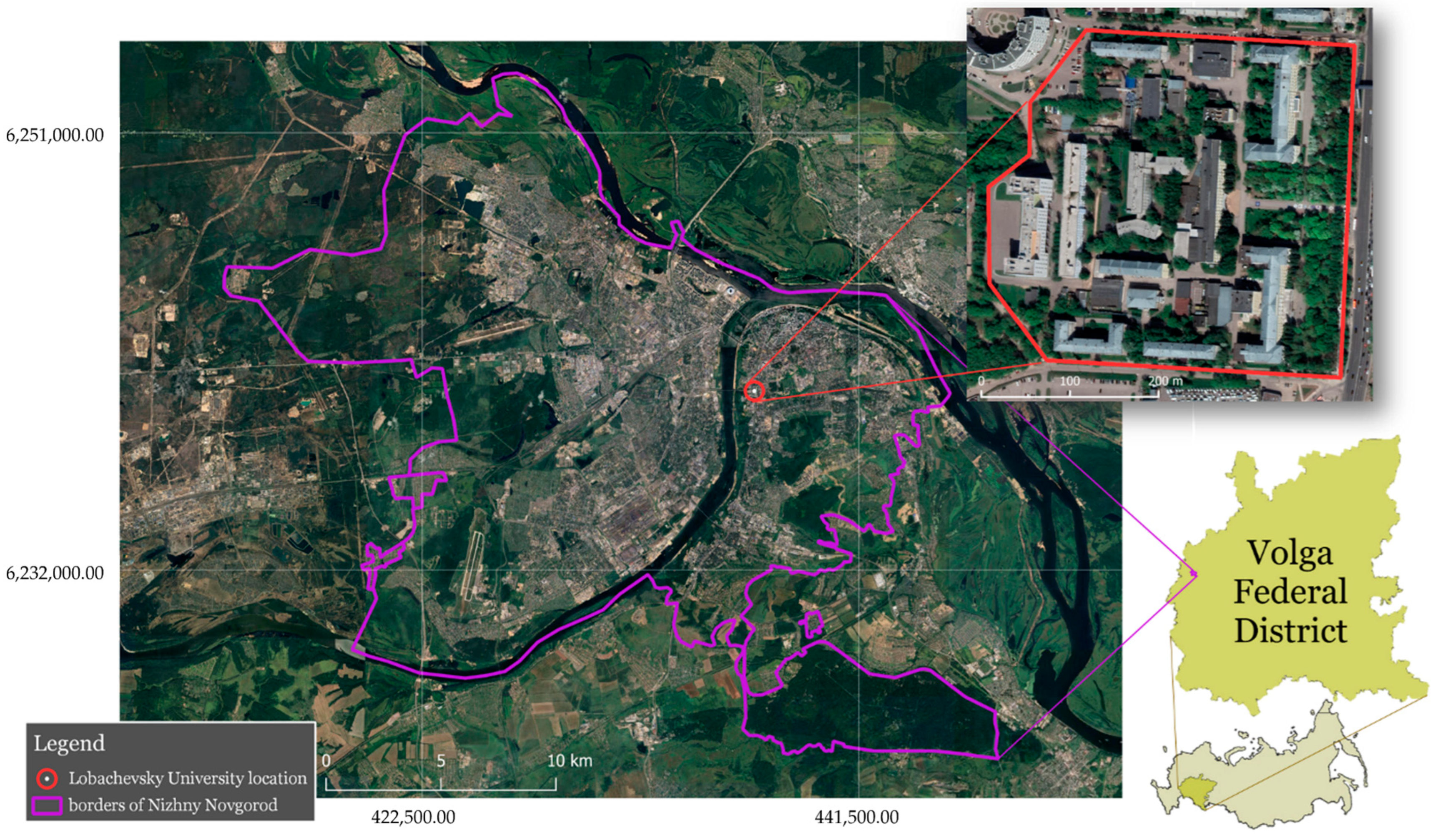
The study area encompassed the Lobachevsky State University of Nizhny Novgorod campus (56°17′54″ N, 43°52′56″ E) in Nizhny Novgorod City, Russia. Situated within a temperate climate zone characterized by moderate continental conditions, the campus has an elevation ranging from 173 to 225 m above sea level and covers a total area of 13.07 hectares. Figure 1 displays the specific location of the study area.

2.2. Input Data and Preprocessing

2.2.1. Field Survey

During the summer season of 2022, a comprehensive inventory of the campus’s woody vegetation was carried out utilizing the i-Tree methodology, as detailed in the guide “Understanding i-Tree: Summary of Programs and Methods” [69].
The survey identified 1887 trees (97% deciduous and 3% coniferous) belonging to 32 species (Table 1). Ground survey indicated that hawthorn (Crataegus laevigata (Poir.) DC.), ash-leaved maple (Acer negundo L.), and birch (Betula pendula Roth) are the dominant species. The stand density is 139 trees per hectare, with an average tree height of 14.41 m and an average diameter at breast height of 21.4 cm.

2.2.2. Remote Sensing Data

The study area was overflown using a DJI Phantom 4 Multispectral UAV (DJI P4M; DJI, Shenzhen, China) equipped with a multispectral camera. This camera included six 1/2.9″ CMOS sensors: one RGB and five monochrome sensors with the following spectral ranges: blue (450 nm ± 16 nm), green (560 nm ± 16 nm), red (650 nm ± 16 nm), red edge (730 nm ± 16 nm), and near-infrared (840 nm ± 26 nm). For this study, we utilized imagery from a flight mission completed on 13 July 2022, which was executed in automatic mode with predetermined parameters using the DJI Ground Station Pro (DJI, Shenzhen, China) flight mission planner. The operating parameters are detailed in Table 2.
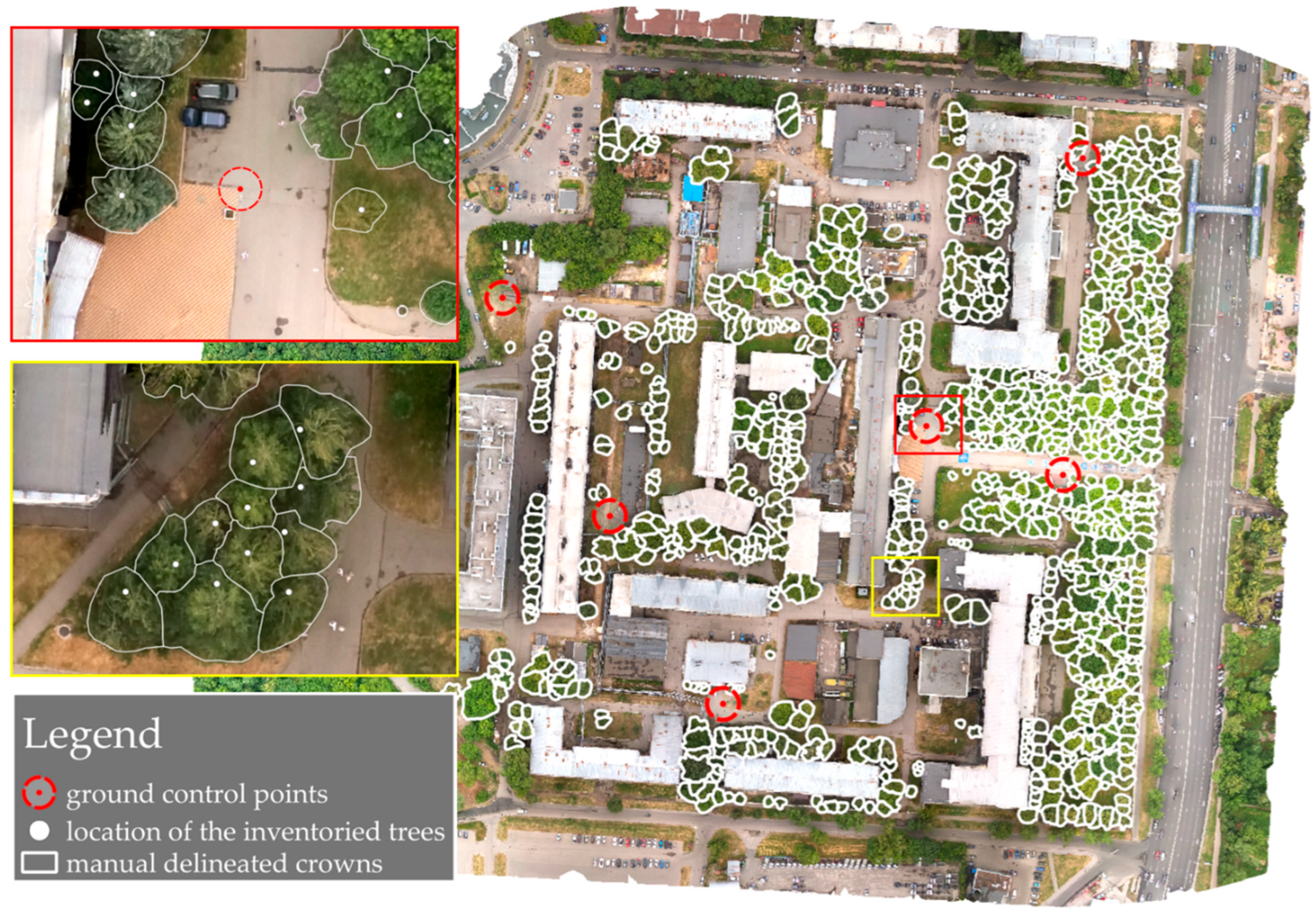
A total of 2457 images were utilized in this research. To reduce geolocation error, six Ground-Control Points (GCPs) were established (Figure 2) using a PrinCe i30 GNSS receiver (CHCNAV, Shanghai, China) connected to a base station network. An ordinary RGB orthomosaic and its corresponding Digital Surface Model (DSM) were generated using the OpenDroneMap toolkit with the use of GCP positions. The Digital Terrain Model (DTM) was prepared based on the altitude coordinates of auxiliary control points, also derived using the GNSS receiver. The spatial resolution for both the RGB orthomosaic and the digital models was 10 cm/pixel.
The normalized Digital Surface Model (nDSM) was obtained by subtracting the DTM from the DSM:
n D S M = D S M D T M ,
which was then cropped to the boundaries of the UNN campus.
Multispectral orthomosaic was aligned using a thin-plate spline transformation with the nearest neighbor method of oversampling via QGIS (3.40.8) software. Then, the Normalized Difference Vegetation Index (NDVI) was calculated using the red and near-infrared bands:
N D V I =   N I R R E D N I R + R E D ,
where NIR represents the near-infrared band and RED represents the red band.
A Gaussian filter (n = 75, σ = 2) was applied to the resulting raster with NDVI values to exclude all tall non-vegetation objects (such as buildings, cars, heating mains and pipes, street lights, etc.) and reduce raster interpretation errors (individual bright pixels that are artifacts caused by the reflecting surface). Finally, pixels for which NDVI was <0.5 were discarded from the nDSM, as NDVI values higher than 0.5 typically characterize dense and/or intensively vegetating plants. This transformation results in the creation of the CHM:
C H M p x = n D S M p x i f   N D V I p x 0.5 i f   N D V I p x < 0.5     ,
where px is a pixel matching for each raster layer.
Thus, a single CHM was prepared, which was subsequently utilized in all the considered segmentation algorithms. The procedure for CHM creation is illustrated in Figure 3.

2.2.3. Manual Tree Segmentation

Manual digitization of tree crowns was performed using Quantum GIS (3.40.8) software within the study area, with a focus on the field inventory data. Tree crown recognition was constrained by the visual interpretability from the UAV flight altitude. Crown boundaries were delineated for each tree individually, considering the spatial position of its trunk. For trees with multiple stems, the crowns of each separate trunk were merged into a single crown. This manual digitization process resulted in 956 reference crowns (manually delineated; Figure 2) in a horizontal projection format.
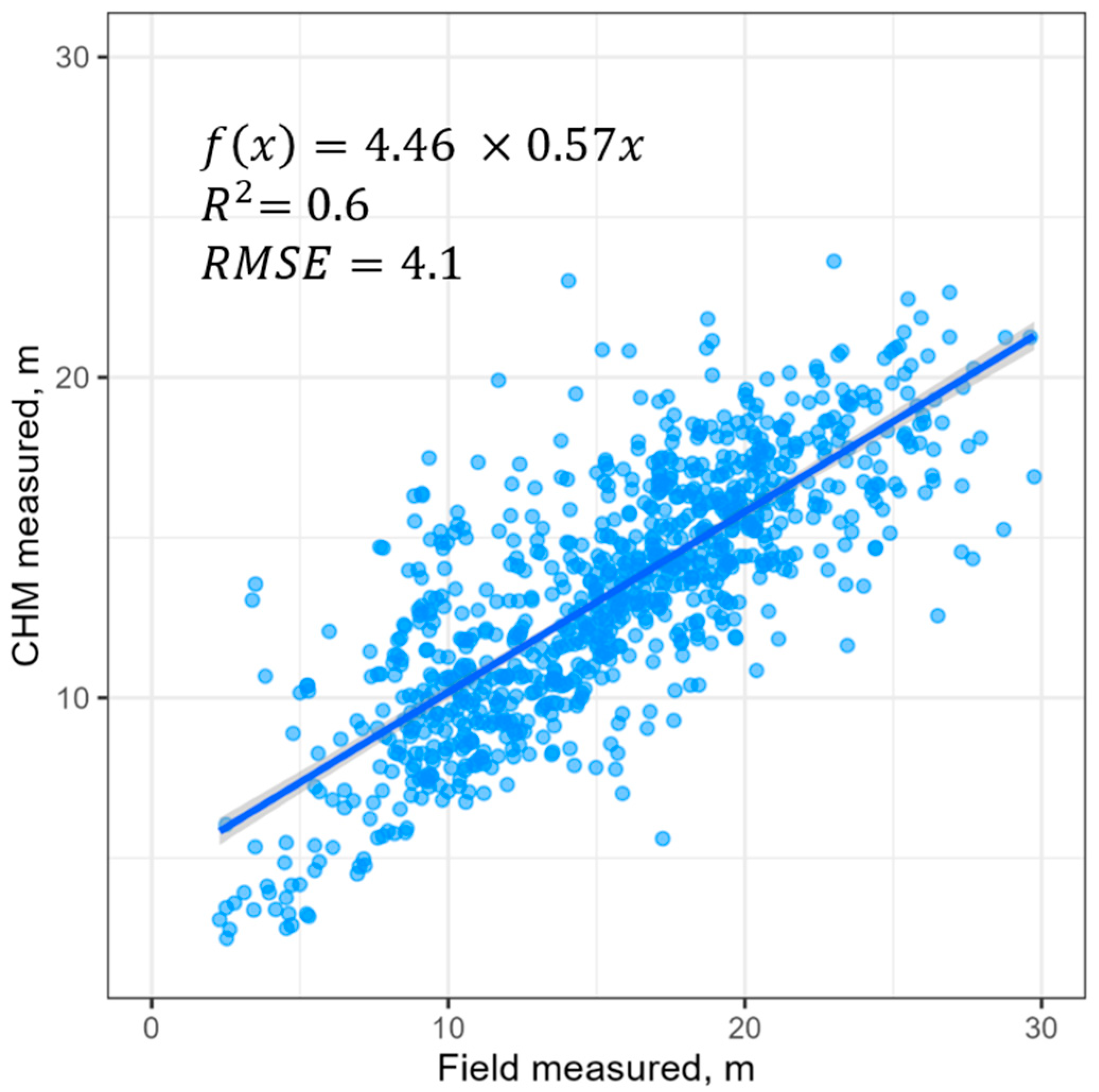
For subsequent calculations and analysis, the initial set of trees was filtered to retain only the tallest tree within each polygon. Based on the characteristics of this filtered set of trees and their digitized crowns, the following empirical parameters were calculated: a minimum tree height of 2.51 m and a maximum crown diameter of 21.6 m. A regression model was also fitted to describe the dependence of crown width on tree height: crown width = 3.192 + height × 0.2414 (R2 = 0.24). A comparison between the heights obtained from the filtered set of crowns and those derived from the CHM data reveals that the CHM is less accurate for tall trees and generally yields slightly lower measurements than the field data (Figure 4).

2.3. Individual Tree Segmentation Algorithms

CHM-based image segmentation methods were employed to automatically identify individual trees and their crown boundaries. Computations were performed in the R environment utilizing the lidR [70] and ForestTools [71] packages. Although all the described algorithms differ, they are all semi-automated and necessitate user involvement. Brief descriptions of the methods used are provided below.

2.3.1. Original Watershed Algorithm (Watershed)

The Watershed algorithm is a region-based method of image segmentation. Its original concept was introduced by Digabel and Lantuejoul in 1978 [72] and it found wide application in mathematical morphology [73]. The modern version of the algorithm was proposed by Vincent and Soille in 1991 [74], which proved to be faster and more accurate than the original one. The basic concept of the modern version of the Watershed algorithm for CHM segmentation involves the decomposition of the image into catchment basins and can be described as follows.
Initially, local maxima are searched for within the image, serving as starting points for the expansion of catchment basin boundaries. When the boundaries of expanding neighboring catchment basins touch, a dam is formed between them. This implementation of the method is known for its sensitivity to image noise, which often leads to “over-segmentation” [27,39,75].
This method is implemented in the lidR (4.2.0) package. User-controlled algorithm input parameters are presented in Table 3.

2.3.2. Marker-Controlled Watershed Segmentation Algorithm (MCWS)

The Marker-Controlled Watershed Segmentation algorithm, proposed by Meyer and Beucher in 1990 [76], is a modification of the previous algorithm designed to address oversegmentation by utilizing a prior labeled image [21]. This segmentation process occurs in two stages. Initially, a Variable Window Filter (VWF) algorithm [77] is employed to identify treetops as local peaks within the CHM. The VWF retrieves the height value of each pixel and generates a moving window, the size of which is determined by height data:
C W = R E G i n t +   R E G s l o p e × H ,
where CW represents crown width, REGint and REGslope are coefficients of linear regression, and H is the height of the current CHM pixel.
If there are no pixels with higher values within the searching window, the middle one is marked as the local maximum. A threshold value is used to exclude low vegetation heights. The output of the VWF algorithm is the location of the detected treetops. The second step is segmentation based on the original watershed algorithm, which accepts both the CHM and the treetop locations prepared through the use of VWF.
This method is implemented in the ForestTools (1.0.2) package. User-controlled algorithm input parameters are presented in Table 4, where default values correspond to linear regression and field measurements for stands on the campus (Section 2.2.3).

2.3.3. Marker-Based Regional Growth Algorithm (Dalponte)

Dalponte and Coomes developed another segmentation technique in 2016 [66], an adaptation of the region growing approach [78]. This algorithm works by gradually joining surrounding pixels that meet specific criteria to the starting point. The approach begins with a CHM smoothing procedure to reduce the number of potential local maxima, followed by further local maxima detection with VWF. Every detected local maximum is regarded as a treetop. If specific conditions are met, it joins nearby pixels in the CHM until there are no more neighbors.
This method is implemented in the lidR (4.2.0) package. User-controlled algorithm input parameters are presented in Table 5.

2.3.4. Improved K-Nearest Neighbor Algorithm (Silva)

The following approach was developed by Silva et al. in 2016 [65]. This segmentation technique’s main feature is using the Voronoi tessellation method for crown delineation. The algorithm begins by receiving treetop locations (detected with VWF) and then computing the crown buffer for each treetop. The diameter of the crown buffer is determined by the height of the treetop pixel multiplied by a fixed value (max_cr_factor). Subsequently, each individual tree crown is delineated using centroid Voronoi tessellation, constrained by the crown buffers. Finally, a threshold is applied to exclude low-lying noise [65].
The method is implemented in the lidR (4.2.0) package. The user-controlled algorithm inputs are presented in Table 6.

2.4. Accuracy Evaluation

To evaluate the accuracy of the algorithms, the Intersection over Union (IoU) metric was used. This metric was calculated for each intersection between manually delineated (MD) crowns (“ground-truth”) and automatically segmented (AS) crowns according to the following equation [39,62,63]:
I o U M D ,   A S   =   M D     A S M D     A S ,
where MD represents a manually delineated crown, and AS denotes an algorithmically recognized crown.
Based on the obtained index value, each pair of manually delineated and algorithmically segmented crowns was assigned to one of three categories based on their mutual arrangement:
  • An AS crown was classified as a “true positive” (TP) if its IoU > 0.5;
  • An AS crown was classified as a “false positive” (FP) if its IoU ≤ 0.5;
  • An MD crown was classified as a “false negative” (FN) if its IoU ≤ 0.5.
Conceptually, this can be represented as follows. Initially, all MD and AS crowns are assigned corresponding FN and FP statuses. If the IoU value for an MD-AS pair is calculated to be greater than 0.5, the FN status is annulled, and the FP status is transformed into TP.
Finally, for each automatic segmentation, precision, recall, and F-score metrics [79,80] were calculated:
P r e c i s i o n = T P T P + F P
R e c a l l = T P T P + F N
F = 2 × P r e c i s i o n × R e c a l l P r e c i s i o n + R e c a l l
Precision indicates the user’s accuracy or the redundancy degree of segmentation (commission error rate). Recall represents the producer’s accuracy or the degree of under-segmentation (omission error rate). The F-score, which is the harmonic mean of precision and recall values, signifies overall segmentation performance [63,81].

2.5. Parameter Optimization Methods

The selection of optimal parameter configurations for vegetation image segmentation can be framed as a multi-variable function minimization problem, solvable through various multidimensional optimization techniques. The objective was to minimize an error function, defined as L = 1 − F, where F represents the F-score, thereby maximizing the overall segmentation performance. For each parameter θ, we were seeking an optimal value  θ * = arg min θ Θ L ( θ ) from a pre-defined range Θ. We evaluated several common optimization methods, including Grid Search, Random Search, the quasi-Newton method, Conjugate Gradients, the quasi-Newton method with box constraints, the Nelder–Mead method, Simulated Annealing, and the Genetic and Differential Evolution (DE) algorithms [82,83,84,85,86,87,88]. Initial tests on the Watershed segmentation method indicated that the Random Search method and the “DE/local-to-best/1/bin” Differential Evolution strategy yield the best outcomes (Appendix A and Supplementary Materials). Consequently, these two methods were employed to determine the optimal parameter settings for three additional segmentation algorithms.
The optimization algorithms were set to run for a maximum of 2400 iterations, at which point the process was terminated. For all segmentation algorithms, the ranges for parameter optimization (including default, minimum, and maximum values presented in Table 3, Table 4, Table 5 and Table 6) were determined based on a combination of theoretical limits, practical considerations, and preliminary empirical trials. Lower bounds for parameters such as hmin, hmin.xx, and th_tree were set to physically meaningful non-negative values, as negative heights are irrelevant for tree detection. For parameters like sigma (smoothing) or REGslope (crown width dependence), a zero value signifies the absence of an effect or a simplified relationship. Conversely, the upper bounds were established where further increases in parameter values either led to a consistent decrease in segmentation efficiency (e.g., by excessively excluding shorter trees or over-enlarging search radii, thereby increasing False Negatives) or significantly hampered computational feasibility, as was observed with the Grid Search method. This approach aimed to define a balanced and effective search space for optimization, reflecting both the algorithms’ theoretical underpinnings and their practical application constraints. It is important to note that the algorithms, including the preliminary treetop search, optimized the parameters of this stage independently, despite having identical functions and computing ranges.
The computations were performed on a computer with the following characteristics: Intel Core i7-11700F processor (Intel, Santa Clara, CA, USA), 4096 GB SSD, NVIDIA GeForce RTX 3070 graphics card (NVIDIA, Santa Clara, CA, USA).

2.5.1. Random Search

The random search (RS) method is one of the simplest “Exact methods of global optimization” used to solve parametric optimization problems, including multidimensional ones. However, the possibilities of applying random search usually become greatly limited as the number of variables being simultaneously optimized increases. In our research, we used the so-called “pure” Random Search, i.e., with independent uniform selection of parameter values for each iteration [68].
While the RS algorithm was running, its characteristics were recorded for each iteration, including the segmentation algorithm parameters, time spent in minutes, and the values of precision, recall, and F-score metrics.

2.5.2. Differential Evolution

Differential Evolution methods have been successfully applied to solve scientific and technological problems for over 25 years. These stochastic algorithms numerically optimize a function with a set of variables. The optimization process can be represented as follows: random points are placed uniformly in a multidimensional space, forming an initial “population” whose size remains constant throughout the optimization process. Subsequently, evolutionary processes (mutation, crossover, and selection) are simulated for the initial population, guiding the initial vectors toward the global optimum. Once the maximum number of generations is reached, the algorithm halts and provides a solution in the form of the best vector [83,89,90].
The DE algorithms are implemented in the DEoptim (2.2-8) package of the R environment [91]. We applied the ‘DE/local-to-best/1/bin’ strategy [91,92] to optimize the parameter values of the algorithms with twenty population members (this amount was consistent across all four segmentation methods). We used standard values of crossover probability (CR = 0.5) and differential weighting factor (F = 0.8) during our study. This strategy implies mutation procedure according to the equation:
v i , g = o l d i , g + b e s t g o l d i , g + x r 0 , g + F × ( x r 1 , g x r 2 , g )
where xr0, xr1, and xr2 are the three members of the population chosen randomly, oldi,g is the i-th member of the previous population, and bestg is the best member of the previous population.
The option of parallelization of calculations with the package parallel (4.5.0) was used to speed up the computations. During the DE algorithm’s execution, the characteristics of each “organism” at each generation, as well as the generations themselves, were recorded. Three algorithms, including the preliminary treetop search, optimized their parameters independently of each other.

3. Results

3.1. Field Data and Manually Delineated Crown Characteristics

Manual digitization of orthomosaics yielded 956 reference crowns. This number is significantly lower than the total number of stems due to two primary factors. Firstly, shrubs are prevalent in the campus landscape, with individual crowns represented by multiple stems. Secondly, many smaller stems are situated beneath the canopies of taller trees, rendering them undetectable on the orthomosaic. Consequently, the average characteristics of manually delineated crowns differ: their average height is 15.5 m, and the average diameter at breast height (dbh) is 31.2 cm (Figure 5). The prevalent species also vary, with Betula pendula, Acer negundo, and Tilia cordata being the most common.

3.2. Individual Tree Segmentations Based on Default Parameters

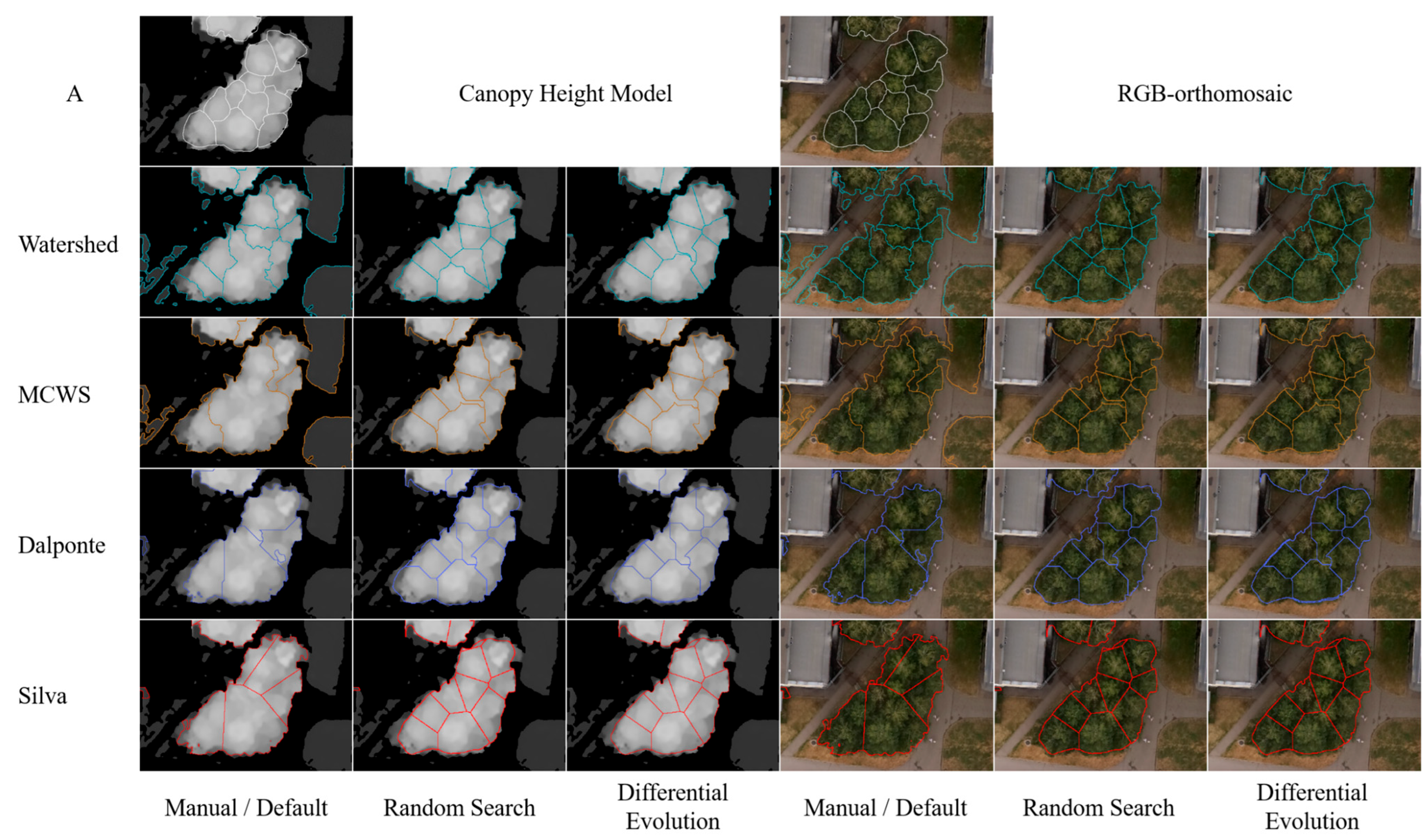
The results of CHM segmentation by Watershed, MCWS, Dalponte, and Silva algorithms using default parameters are presented in Table 7. Examples of segmentation for a small tree stand site are shown in Figure 6. The VWF-based segmentation methods demonstrated slightly higher accuracy with default parameter values compared to the Watershed method, which does not require pre-detected treetops. The Silva (TP = 187, F-score = 0.2287) and Dalponte (TP = 176, F-score = 0.2153) methods yielded the best results for crown detection. All algorithms produced a high number of false negatives and a low recall value, indicating significant image undersegmentation (Figure 6). The Watershed algorithm also exhibited a high number of false positives and, consequently, a low precision value, indicating a high degree of redundant segmentation against the background of general undersegmentation (high variation in segment sizes).

3.3. Parameter Optimization for Segmentation Algorithms

3.3.1. Optimization Through the Random Search

All four segmentation methods showed improved crown recognition quality when their parameters were optimized using Random Search (Table 8). Following parameter optimization, the Silva algorithm achieved the best result (TP = 332, F-score = 0.3807), with a 0.152 improvement in F-score over the default parameters. MCWS showed the next best result (F-score = 0.3783), while Dalponte and Watershed algorithms were least accurate and close in their performance (F-score is about 0.35). However, the Watershed algorithm demonstrated the largest increase in efficiency among the presented algorithms (0.2 F-score points). It is noteworthy that the difference in accuracy among the four algorithms was minimal, within the range of 0.03 F-score points (corresponding standard deviation is 0.0152).
The optimization results for the smoothing parameter in the Dalponte and Silva algorithms (Sigma ∈ (9; 10)) differ significantly from those of the Watershed (Sigma ≈ 3) and MCWS (Sigma ≈ 5) methods. Furthermore, the optimized coefficients for the regression equation varied across all three algorithms employing preliminary treetop detection. Only the REGslope parameter for the Dalponte and Silva algorithms showed comparable values (REGslope ≈ 0.07–0.09). The MCWS algorithm’s slope for the crown width-to-height dependence was approximately eight times lower. For all three algorithms, the regression parameters diverged considerably from the empirical relationship estimated from field data, with the slope differing by more than three times.
All four segmentation methods demonstrated a slight decrease in undersegmentation (FN), leading to a general increase in correct recognitions (TP, Table 8). For the MCWS, Dalponte, and Silva algorithms, the number of oversegmentation cases (FP) changed only slightly. In contrast, optimizing the parameters for the Watershed algorithm resulted in a significant reduction in false positives. Notably, after optimization, there was a relative alignment of FP and FN cases, leading to a corresponding alignment of Precision and Recall metrics.
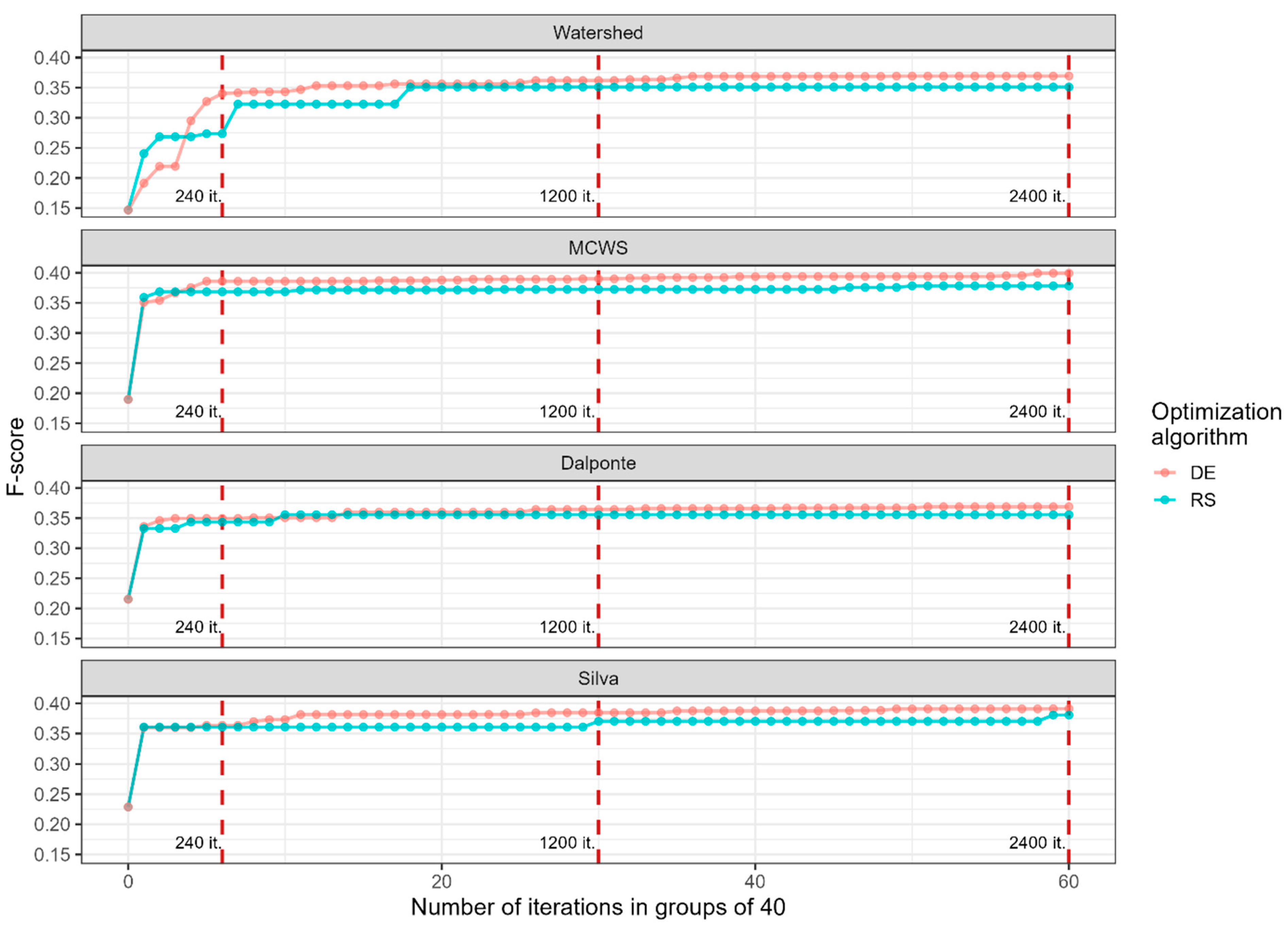
The speed of determining optimal parameter configurations for more efficient crown delineation using Random Search varied across different algorithms. For instance, within the first 40 iterations, the MCWS, Dalponte, and Silva algorithms showed a sharp increase in accuracy, followed by a slow increase in efficiency (Figure 7). The Watershed algorithm also demonstrated a rapid increase in the initial stage, with a significant further increase during subsequent iterations of Random Search. All algorithms reached a relatively stable plateau near 800 iterations (position 20 on the axis of the abscissa, considering the grouping), with subsequent smoother changes towards a higher F-score.
The speed of CHM segmentation into individual crowns is influenced by both the segmentation algorithm and its parameters, affecting the duration of individual segmentations and the overall parameter optimization process (Table 9). The Watershed algorithm exhibits the minimal average segmentation time at 1.94 min. Conversely, the Dalponte algorithm is the slowest, with an average execution time per segmentation of 12.15 min, approximately three times longer than the other three algorithms. Consequently, the total time dedicated to parameter optimization is least for the Watershed algorithm and most for the Dalponte algorithm.

3.3.2. Optimization Through the Differential Evolution

All four segmentation methods improved the quality of crown recognition when their parameters were systematically optimized with Differential Evolution (Table 10). Following parameter optimization, the MCWS algorithm showed the best result (TP = 369, F-score = 0.3994), achieving a 0.21 improvement in F-score over the default parameters. The Silva algorithm was very close (F-score = 0.3912), while the Dalponte and Watershed algorithms exhibited the lowest final accuracy, and their performance was very close (F-score ≈ 0.369). The Watershed algorithm demonstrated the highest increase in efficiency (0.223 F-score points) among the presented algorithms. Similar to Random Search optimization, the difference in accuracy among the four algorithms was minimal, within the range of 0.03 F-score points (corresponding standard deviation is 0.0154).
The optimization results for the smoothing parameter in the Watershed, Dalponte, and Silva algorithms (Sigma ∈ (9; 11)) differ significantly from the MCWS method (Sigma ≈ 5). The optimized coefficients for the regression equation varied across all three algorithms employing preliminary treetop detection, with only the REGslope parameter for the MCWS and Dalponte algorithms showing comparable values (REGslope ≈ 0.11–0.12). For the Silva algorithm, the slope of the dependence of crown width on height is approximately four times lower. For all three algorithms, the regression parameters differ significantly from the empirical relationship estimated from field data, with the slope differing by more than two times.
All the algorithms slightly decreased undersegmentation, leading to a general increase in correct recognitions (Table 10). For the MCWS, Dalponte, and Silva algorithms, the number of oversegmentation cases remained almost unchanged. In contrast, optimizing the parameters of the Watershed algorithm led to a significant reduction in false positives. A relative alignment of FP and FN cases can also be observed. Likewise, the visualization of segmentation can be overseen in Figure 7.
The rate of parameter optimization during differential evolution also differs between segmentation algorithms. The MCWS, Dalponte, and Silva algorithms show a sharp increase in accuracy after the first generation during evolution, followed by a slow increment (Figure 7). The Watershed algorithm also demonstrates a fast increase in the initial stage, with a significant further increase during subsequent generations of DE. After the 15th generation, all algorithms attain a comparatively stable plateau, followed by smoother shifts towards a higher F-score.
The speed of CHM segmentation into individual crowns is influenced by both the segmentation algorithm and its parameters, affecting the duration of individual segmentations and the overall parameter optimization process (Table 11). The Watershed algorithm exhibits the minimal average segmentation time at 1.73 min. Conversely, the Dalponte algorithm is the slowest, with an average execution time per segmentation of 5.89 min, approximately three times longer than the other three algorithms. Consequently, the total time dedicated to parameter optimization is least for the Watershed algorithm and most for the Dalponte algorithm. The MCWS and Silva algorithms demonstrated comparable segmentation rates.

3.3.3. The Optimization Outcomes Comparison

The trajectories of accuracy and efficiency improvement for the four algorithms considered, using the two optimization methods, are shown in Figure 7. The graph indicates that optimization via Differential Evolution achieved higher efficiency values compared to the Random Search approach. The efficiency discrepancy between the two optimization methods was 0.0211 for the MCWS algorithm, 0.0184% for the Watershed algorithm, 0.0134% for the Dalponte algorithm, and 0.0105% for the Silva algorithm. After 240 iterations (6 generations for the DE), all algorithms showed stable efficiency growth at a relatively high level, irrespective of the chosen optimization method. A stable, though small, gap between the different optimization methods formed closer to the 1000th iteration (25 generations for the DE).
We also analyzed how performance metrics depend on specific parameters of the segmentation algorithms. We considered all parameter values sampled during the RS and DE procedures and fitted linear models relating the F-score to individual parameters. Table 12 presents the main statistical indicators of these linear models. The identified dependencies between parameter values are mostly significant (p < 0.05), with notable exceptions: the parameter hmin for the Silva algorithm with the RS optimization (p = 0.241); parameter hmin.tt for the MCWS algorithm (p = 0.076); and parameters sigma (p = 0.08) and th_cr (p = 0.455) for the Dalponte algorithm with the DE optimization. For each particular parameter value, the F-score can vary significantly depending on the values of other parameters, emphasizing the need for joint optimization of the segmentation algorithm parameters.

3.3.4. Ablation Study

To evaluate the isolated contribution of specific optimized parameters to the overall segmentation performance, an ablation study was conducted [93]. This involved systematically resetting individual parameters to their default values and observing the consequent impact on the F-score. The performance degradation ( F ) was calculated using the following formula:
F i = F θ F ( θ i ) ,
where  F θ represents the F-score achieved with all parameters at their optimized values (taken from Table 10), and  F ( θ i ) is the F-score obtained when a single parameter is reset to its default value (from Table 3, Table 4, Table 5 and Table 6) while all other parameters remain at their optimized settings. This approach specifically quantifies the individual parameter’s contribution to the optimized F-score rather than evaluating the optimization method itself.
The results indicate that for the Dalponte, Silva, and MCWS algorithms, the Sigma parameter (controlling CHM smoothing) exerts the strongest influence on the final F-score when its value is reverted to default (Figure 8). Specifically, the Dalponte, Silva, and MCWS algorithms showed F-score impairments  F of 0.0786, 0.1736, and 0.1699, respectively. For the Watershed algorithm, the tol parameter proved to be more critically important, with its default value leading to a significant F-score worsening  F of 0.2405. Notably, the effect of the Sigma parameter on the Watershed algorithm was also substantial, yielding a  F of 0.1123, which is greater than its impact on the MCWS algorithm.
Conversely, the parameters with the least influence in this ablation study were ext for the Watershed algorithm, hmin.tt for the MCWS algorithm, th_cr for the Dalponte algorithm, and exclusion for the Silva algorithm. For all parameters across the four algorithms, the calculated  F values were positive, confirming that reverting any optimized parameter to its default consistently led to a decrease in the F-score.

4. Discussion

In this study, we investigated how different parameter selection methods affect tree recognition quality using four common segmentation algorithms: Watershed, Marker-Controlled Watershed, Dalponte, and Silva. We broadly distinguish two parameter selection approaches: passive, where parameters are set using default values and/or field data, and active, where optimal parameter configurations are determined through manual or algorithmic search. Our results indicate that adopting an active parameter selection substantially improved the overall performance of all segmentation algorithms. Initially, the Silva (F-score = 0.2287) and Dalponte (F-score = 0.2153) methods showed higher performance than MCWS (F-score = 0.1896) and Watershed (F-score = 0.1468), potentially suggesting greater “universality” in segmenting vegetation images from various regions. However, after optimization, all studied methods exhibited a similar segmentation pattern with only minor differences in overall efficiency (within the range of 0.3 F-score points). This suggests that the key to accurate tree detection lies not in the segmentation method itself, but in its preliminary tuning and optimization.

4.1. Tuning the Values of the Segmentation Algorithm Parameters and Searching for the Optimal Configuration

The optimization procedure enabled the achievement of a more optimal parameter configuration after only 40 iterations (for the MCWS, Dalponte, and Silva algorithms), leading to an efficiency increase of 0.11–0.16 F-score points and excluding the human factor’s influence on input parameter value selection (Figure 7). After 300 iterations, segmentation efficiency saw an improvement of 0.12–0.19 F-score points. Consequently, our study’s results indicate that conducting reasonable optimization with random selection of input parameter values can enhance the overall effectiveness of individual tree crown detection and delineation algorithms. Furthermore, applying Differential Evolution may prove to be a sound solution in the long run (>1000 iterations), while Random Search can provide an approximate solution after just a few dozen iterations.
In the context of studying tree vegetation, a common practice for working with such algorithms involves choosing parameter values based on the interpretation of field measurements. For instance, Popescu and Wynne [77] proposed using a linear regression with a quadratic model (separate models for deciduous, coniferous, and mixed forests), derived from measurements of 424 trees, to predict crown width based on tree height. Technically, their research integrates these regression models into the Local Maximum Filtering (LMF) function [77], enabling the prediction of crown boundaries within the CHM. The core ideas of this approach have been applied in studies focused on tree detection using LMF [10,46].
With the development of more advanced CHM segmentation methods, specifically adapted for delineating tree crowns (e.g., [65,66]), additional empirical parameters have been introduced to enhance canopy segmentation accuracy. Silva et al. [65] estimated the expected tree crown diameter as 60% of its height, based on preliminary field observations. This relationship is incorporated into their segmentation algorithm as a specific parameter, max_cr_factor, with a default value of 0.6. Silva and colleagues also suggested excluding all pixels with height values below a predetermined, fixed proportion of the maximum height of the detected tree, a coefficient termed exclusion. They proposed a default value of 0.3 for this parameter in their algorithm.
A somewhat different situation arose with the algorithm proposed by Dalponte and Coomes [66]. In their work describing the algorithm’s principles, the authors do not mention specific values for key parameters used to delineate crowns, only noting that these parameter values “should be defined by user”. However, to compare our results with a hypothetical benchmark, we followed Pu et al. [45], Hastings et al. [47], and Tatum and Wallin [44]. We defined default values for parameters describing the inclusion of neighboring pixels into the crown, th_seed and th_cr, as 0.45 and 0.55, respectively.
The most complex and ambiguous situation regarding parameter selection arises with watershed segmentation algorithms, where key threshold values are often not even mentioned when the algorithm is used for tree crown delineation (e.g., [9,39,43]). This significantly complicates the decision-making process for determining optimal parameter values.
It is most probable that in cases where the aforementioned algorithms are applied, parameter values are manually chosen by an operator. Some studies emphasize the screening of window or kernel sizes for LMF algorithms, without detailed descriptions of further parameter tuning [33,46,52,63]. Zhang et al. [94] employed a “trial-and-error” method to determine optimal segmentation algorithm parameter configurations during testing and parameter adjustment. Conversely, utilizing machine learning models for individual tree detection and crown delineation obviates the need for parameter value optimization due to the fundamental operational principles of these models, which typically render the model’s decision-making process not entirely transparent. From the current perspective, comparing machine learning models with “embedded” optimization solutions to simpler, user-configured segmentation algorithms appears unconvincing.
We employed the Random Search and Differential Evolution optimization algorithms to identify the optimal parameter values. For most parameters, the optimized values differed from the default reference values. For instance, optimizing the Dalponte algorithm’s parameters using Random Search yielded a configuration where the th_seed parameter was approximately 0.195 (−0.255 compared to the default value) and the th_cr parameter was approximately 0.15 (−0.4). In contrast, applying Differential Evolution resulted in values of 0.06 (−0.39) for th_seed and 0.55 for th_cr, with the latter parameter’s optimized value matching the default to three decimal places.
For the Silva segmentation algorithm, the values of the parameters max_cr_factor and exclusion showed relatively similar optimization regardless of the method used, with differences not exceeding 5%. However, compared to the default values, the optimized max_cr_factor parameter received lower values (−0.15 to −0.20), while the exclusion parameter received higher values (+0.12 to +0.15). For the Watershed and MCWS methods, assessing the correspondence between optimized and default parameters was difficult due to a lack of information on reference values, underscoring the need for active parameter selection.
This critical role of parameter optimization was further quantified by our ablation study (Section 3.3.4). The study demonstrated that for Dalponte, Silva, and MCWS algorithms, the Sigma parameter was particularly influential, as reverting it to its default value resulted in the most substantial F-score degradation. Similarly, for the Watershed algorithm, the tol parameter exhibited the strongest individual impact on performance.

4.2. The Effect of Parameters on the Accuracy of Tree Delineation

The determination of the actual impact of each parameter on segmentation efficiency is complicated by the fact that our chosen optimization methods operate within a multi-dimensional parameter space. In this space, each unique parameter contributes to an efficiency increase only in conjunction with other parameters. This notably explains the exceptionally wide spread of efficiency metrics observed for specific sigma values during the optimization of other key parameters (Figure 9), and a similar situation exists for other parameters.
A somewhat ambiguous situation arises concerning the smoothing of the CHM and the sigma parameter, which determines the strength of this smoothing. Initial tests indicate that the model’s segmentation effectiveness improves with lower smoothing strength values, assuming other parameter values are set to “default” (Figure 9). However, the results from simultaneously optimizing all parameters in a multi-dimensional space did not reveal a strict relationship between segmentation effectiveness and CHM smoothing strength, even when employing Differential Evolution methods where individual parameters contributing to increased tree canopy boundary recognition accuracy could be maintained across multiple generations. This issue likely deserves further detailed investigation.
In other similar studies, smoothing of the CHM is frequently employed [11,65] to fill in “empty” pixels [32], enhance the accuracy of tree delineation in broadleaf forest conditions [45], and address crown oversegmentation [75]. Fujimoto et al. [67] also highlight the potential use of a Gaussian filter for smoothing Digital Terrain Models. Conversely, Hastings et al. [47] point out the experimentally identified negative effects of such smoothing, which can diminish the effectiveness of crown delineation. Zhen et al. [20] identify “extraction, interpolation, and smoothing procedures” as drawbacks of raster-based methods that may lead to information loss or other potential errors, a concern also raised by Silva et al. [65], who utilized both smoothed and unsmoothed versions of the CHM.
Concurrently, our findings demonstrate that even the application of a straightforward segmentation algorithm, such as the Watershed method, can yield competitive results compared to more complex ones. We hypothesize that our “optimized” parameter value sets may represent local extrema or heuristic solutions. This could explain, for instance, why the optimal values of key parameters, like the coefficients of the regression equation for treetops, obtained by applying different optimization methods may differ significantly within the same segmentation method (Figure 10). Therefore, we believe that to find the best solution, multiple optimization procedure launches or increases in sample size are required.
Our findings indicate that excessive generalization and the use of default parameter values, including those derived from empirical data, prevent segmentation algorithms from achieving maximum efficiency. It is important to emphasize that the optimized regression coefficient values do not correspond to those estimated from field observations (Figure 10), suggesting that empirical data are not fully suitable for describing and analyzing digital models of the corresponding plant communities.
The specific optimized parameter sets derived from the Lobachevsky State University campus are intrinsically data-driven and thus highly tailored to the unique characteristics of our UAV-derived CHMs and local vegetation structure. This data-specific optimization, especially given the absence of explicit mathematical regularization terms in our chosen Random Search and Differential Evolution methods, carries a risk of overfitting to the training data. Therefore, direct transferability of these precise parameter values to other geographical locations, different sensor types, or diverse remote sensing datasets should not be assumed without empirical re-validation. Instead, our study strongly advocates for the application of similar optimization procedures in any subsequent research or practical applications to ensure the highest attainable accuracy and reliability across varied environments and data types. This approach acknowledges the inherent variability in urban forest characteristics and sensor data, promoting a methodologically sound path to robust crown delineation.
In practical applications for broader deployment, this strategy implies that optimization can be performed on a carefully selected subset of the surveyed area where ground truth measurements are available. The parameters optimized on this representative subset can then be reliably applied across larger, ecologically homogeneous local territories or ‘unseen’ landscapes with similar characteristics, thereby extending the utility of the method beyond areas with exhaustive ground truth data.

4.3. An Impartial and Objective Selection of the Best Algorithm for Individual Tree Crown Detection and Delineation

Several studies, including those by Minařík et al. [52], Pu et al. [45], and You et al. [43] have compared different CHM segmentation methods to identify the most appropriate and effective approach for tree detection. These studies indicate that raster-based and point cloud-based approaches have distinct advantages and disadvantages, performing with varying effectiveness under different scenarios. However, an objective comparison of methods necessitates an unbiased selection of parameter values, which can be achieved through a user-independent search for optimal parameter values that may deviate from default settings.
Hastings et al. [47] conducted an iterative search for optimal parameter configurations for the Watershed, MCWS, Dalponte, and Silva algorithms. Similar to our approach, they optimized parameters within the R environment and utilized a comparable set of parameters, ranges, and standard performance metrics. Using default parameters, the F-scores reported by Hastings et al. [47] were 0.08 for Watershed, 0.49 for MCWS, 0.46 for Dalponte, and 0.48 for Silva, which substantially exceeded the performance of these algorithms with default parameters applied to the campus area in our research. The improvement in overall accuracy after parameter tuning was substantial only for the Watershed method (+43%), while the gains for other algorithms ranged from 1% (Silva) to 6% (MCWS). The variation in overall accuracy among the four methods was 5% (0.48–0.53). It is worth noting that Hastings et al. used LiDAR point clouds from NASA’s Goddard LiDAR, Hyperspectral and Thermal remote sensing datasets for implementing segmentation techniques, whereas in our work we used photogrammetric point clouds derived after processing UAV images. Thus, their CHM has a spatial resolution of 1 m, while our CHM has 10 cm. Nevertheless, we strongly believe that this fact does not affect our main findings that follow from this comparison.
Comparing the parameter values obtained by Hastings et al. [47] with our optimization results, we find that the optimal threshold for minimum height for the MCWS algorithm falls within the range of 3.7 to 8.3. However, our findings suggest that treetop detection (hmin.tt) should be set slightly higher than crown detection (hmin.cr), whereas Hastings et al. reported that these values could be nearly identical. For the Watershed, Dalponte, and Silva algorithms, the final values for the corresponding parameters show differences between our results and those of Hastings et al. Furthermore, the optimal parameter values obtained by Hastings et al. varied across different study plots within a single area, underscoring the limitations of generalizing parameter values during extrapolation and highlighting the importance of tuning parameters for each unique tree stand.
It is worth noting that canopy segmentation using different methods requires varying amounts of computational time (Table 9 and Table 11), which may serve as a decisive argument in favor of one segmentation method over another. Evidently, the differences in computational speed among various algorithms are attributable to inherently different approaches to image segmentation and non-identical composition of constituent variables. However, the overall duration and speed of optimization should also be considered crucial factors. The MCWS, Dalponte, and Silva algorithms demonstrate a sharp and significant increase in efficiency after the first dozen iterations during the optimization procedure (Figure 7), after which segmentation effectiveness plateaus with minor improvements throughout the remaining iterations. This observation places the three algorithms on equal footing in terms of crown delineation accuracy. However, the Dalponte method exhibited longer iterations compared to MCWS and Silva methods (Table 9 and Table 11), which may limit its applicability and requires more detailed study. The Watershed algorithm, on the contrary, requires the least computational time among the presented methods but has a relatively slow optimization rate. This might be a consequence of its “versatility” in addressing image segmentation tasks, where crown delineation represents only a specific application.
While our study demonstrates the profound impact of parameter optimization on raster-based segmentation algorithms, it is important to acknowledge that the overall accuracy of individual tree crown delineation can be further enhanced through improvements across the entire processing pipeline. This includes exploring more advanced preliminary data processing techniques for robust vegetation masking, such as object-based image analysis or deep learning-based semantic segmentation, which could provide cleaner inputs to the CHM. Furthermore, the application of sophisticated machine learning and deep learning models for direct canopy detection and instance segmentation, as opposed to traditional raster-based CHM methods, offers another promising direction for future research, potentially circumventing some of the inherent limitations of traditional approaches. Future work could systematically compare the performance gains from such innovations against the benefits of parameter optimization for traditional algorithms, providing a comprehensive understanding of the most effective strategies for urban forest inventory.
5. Conclusions

Drawing upon our findings and those reported by Hastings et al. [47], we propose the following recommendations for the general process of algorithmic tree crown detection from canopy height models:
  • Employ empirical data to establish parameter ranges (instead of fixed values) for subsequent algorithm optimization.
  • Among available alternative methods, prioritize the fastest algorithm; the MCWS demonstrated the best combination of speed and optimizability compared to the Watershed, Dalponte, and Silva.
  • Perform brief optimization using available methods. Even Random Search can yield a better solution after several dozen iterations, while more complex methods will enable finding the global optimum.
Optimizing parameters for vegetation image segmentation algorithms therefore presents a novel perspective on established principles for making methodological decisions in tasks related to individual tree detection and crown delineation. The enhanced accuracy and objectivity achieved through our proposed optimization framework, even for simpler algorithms, translates directly into significant practical utility for subsequent analyses. Such improved segmentation outputs facilitate more precise tree counts, accurate measurements of crown diameters, better estimations of biomass and carbon sequestration, and refined assessments of critical urban ecosystem services. By providing a robust and objective framework for segmentation, our optimized approach supports more informed decision-making in urban forest management, climate change adaptation strategies, and biodiversity conservation efforts. In turn, obtaining more detailed and reliable information about urban tree stands unlocks opportunities for more effective application of remote sensing techniques in assessing ecosystem services. These services not only provide tangible aesthetic benefits but also contribute significantly to creating a comfortable environment and, consequently, a healthy population.

Supplementary Materials

The following supporting information can be downloaded at: https://www.mdpi.com/article/10.3390/f16111655/s1.

Author Contributions

Conceptualization, B.N.Y. and N.I.Z.; methodology, B.N.Y.; software, N.A.I.; validation, N.A.I. and B.N.Y.; formal analysis, B.N.Y.; investigation, N.I.Z.; data curation, N.A.I.; writing—original draft preparation, N.A.I.; writing—review and editing, N.A.I., N.I.Z. and B.N.Y.; visualization, N.A.I.; supervision, B.N.Y.; project administration, N.I.Z.; funding acquisition, B.N.Y. All authors have read and agreed to the published version of the manuscript.

Funding

This study was supported by the Ministry of Science and Higher Education of the Russian Federation (project No. FSWR-2023-0032).

Data Availability Statement

The original contributions presented in this study are included in the supplementary materials. Further inquiries can be directed to the corresponding author. The scripts with all step in data analysis are available in a public repository: https://github.com/basil-yakimov/segmentation-optim/ (accessed on 22 September 2025).

Acknowledgments

The authors would like to acknowledge the Lobachevsky University field crew for implementing the field measurements and obtaining the vegetation data. The authors have reviewed and edited the output and take full responsibility for the content of this publication.

Conflicts of Interest

The authors declare no conflicts of interest.

Appendix A

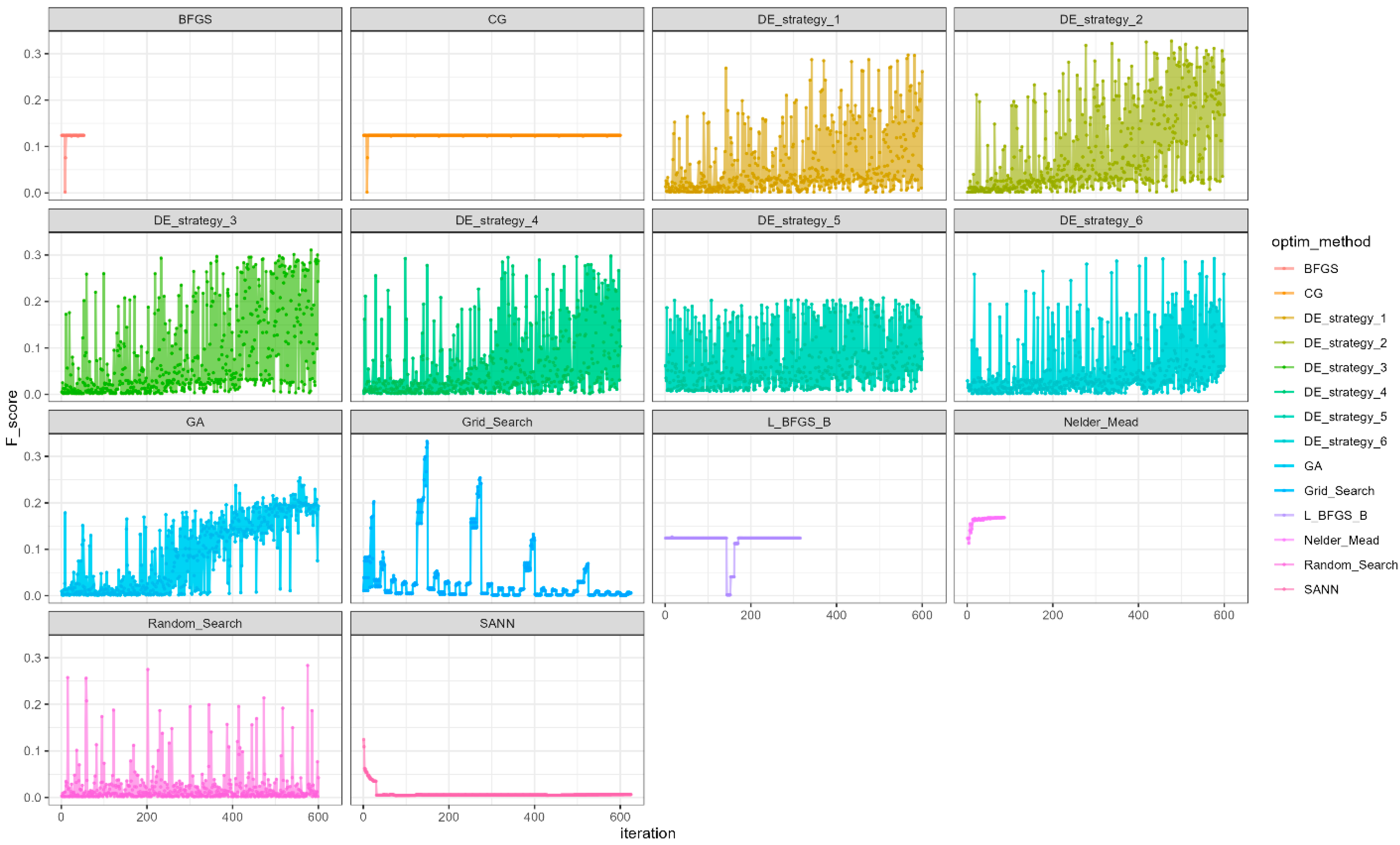
The appendix details a preliminary investigation into various optimization techniques, including Grid Search, Random Search, quasi-Newton method (BFGS), Conjugate Gradients (CG), the quasi-Newton method with box constraints (L-BFGS-B), the Nelder–Mead method, the Simulated Annealing (SANN) method, and the Genetic (GA) and Differential Evolution (DE) algorithms. Given the complexity and time demands of these calculations, the simplest and fastest method, Watershed segmentation, was selected for preliminary results.
Although preliminary results indicated that Grid Search performed best, subsequent tests revealed that its use, while effective for optimizing the Watershed algorithm, was completely impractical for the other three segmentation algorithms under consideration. This was due to the exhaustive search of extreme parameter configurations, which led to excessively redundant segmentation and required hundreds or thousands of minutes of computational time. Therefore, we chose Differential Evolution and Random Search methods for further consideration.
Figure A1. Visualization of the results of applying different optimization methods of the Watershed algorithm, where BFGS—the quasi-Newton method; CG—conjugate gradients method; DE—variuos strategies of Differential Evolution algorithm; GA—Genetic Algorithm; L_BFGS_B—the quasi-Newton method with box constraints method; SANN—the Simulated Annealing method. The algorithmic strategies for differential evolution are denoted as follows: 1—“DE/rand/1/bin”; 2—“DE/local-to-best/1/bin”; 3—“DE/best/1/bin with jitter”; 4—“DE/rand/1/bin with per vector dither”; 5—“DE/rand/1/bin with per generation dither”; 6—“DE/current-to-p-best/1”.
Forests 16 01655 g0a1
Table A1. Ranking of the multidimensional optimization methods used.
RankOptimization MethodF-Score
1Grid Search0.3322
2DE strategy 20.3273
3DE strategy 30.3109
4DE strategy 40.2977
5DE strategy 10.297
6DE strategy 60.2926
7Random Search0.2834
8Genetic Algorithm0.2538
9DE strategy 50.2077
10Nelder Mead0.1683
11L-BFGS-L0.1265
12BFGS0.1241
13CG0.1241
14SANN0.124
15without optimization0.124

References

  1. Millenium Ecosystem Assessment. Ecosystems and Human Well-Being: Synthesis; Island Press: Washington, DC, USA, 2005; ISBN 978-1-59726-040-4, 978-1-59726-039-8. [Google Scholar]
  2. Wang, Y.; Chang, Q.; Fan, P.; Shi, X. From Urban Greenspace to Health Behaviors: An Ecosystem Services-Mediated Perspective. Environ. Res. 2022, 213, 113664. [Google Scholar] [CrossRef]
  3. Chen, J.; Li, H.; Luo, S.; Su, D.; Xie, J.; Zang, T.; Kinoshita, T. Estimating Changes in Inequality of Ecosystem Services Provided by Green Exposure: From a Human Health Perspective. Sci. Total Environ. 2024, 908, 168265. [Google Scholar] [CrossRef]
  4. Zhu, L.; Yang, J.; Ouyang, X.; Xu, Y.; Wong, M.S.; Menenti, M. Street Trees: The Contribution of Latent Heat Flux to Cooling Dense Urban Areas. Urban Clim. 2024, 58, 102147. [Google Scholar] [CrossRef]
  5. Lian, X.; Jiao, L.; Liu, Z.; Jia, Q.; Liu, W.; Liu, Y. A Detection of Street Trees and Green Space: Understanding Contribution of Urban Trees to Climate Change Mitigation. Urban For. Urban Green. 2024, 102, 128561. [Google Scholar] [CrossRef]
  6. Elsadek, M.; Nasr, A.; Guo, L.; Gong, X.; Hassan, A.; Zhang, D. Urban Trees and Elderly Well-Being: Species-Specific Strategies for Thermal Comfort in Heat-Stressed Cities. Forests 2024, 16, 55. [Google Scholar] [CrossRef]
  7. Zhu, W.; Wang, J.; Qin, B. The Relationship between Urban Greenness and Mental Health: A National-Level Study of China. Landsc. Urban Plan. 2023, 238, 104830. [Google Scholar] [CrossRef]
  8. Rötzer, T.; Moser-Reischl, A.; Rahman, M.A.; Pauleit, S. Urban Forest and Urban Microclimate. Forests 2023, 14, 2391. [Google Scholar] [CrossRef]
  9. Man, Q.; Dong, P.; Yang, X.; Wu, Q.; Han, R. Automatic Extraction of Grasses and Individual Trees in Urban Areas Based on Airborne Hyperspectral and LiDAR Data. Remote Sens. 2020, 12, 2725. [Google Scholar] [CrossRef]
  10. Münzinger, M.; Prechtel, N.; Behnisch, M. Mapping the Urban Forest in Detail: From LiDAR Point Clouds to 3D Tree Models. Urban For. Urban Green. 2022, 74, 127637. [Google Scholar] [CrossRef]
  11. Xu, W.; Deng, S.; Liang, D.; Cheng, X. A Crown Morphology-Based Approach to Individual Tree Detection in Subtropical Mixed Broadleaf Urban Forests Using UAV LiDAR Data. Remote Sens. 2021, 13, 1278. [Google Scholar] [CrossRef]
  12. Shahtahmassebi, A.R.; Li, C.; Fan, Y.; Wu, Y.; Lin, Y.; Gan, M.; Wang, K.; Malik, A.; Blackburn, G.A. Remote Sensing of Urban Green Spaces: A Review. Urban For. Urban Green. 2021, 57, 126946. [Google Scholar] [CrossRef]
  13. Laurenz, J.; Belausteguigoitia, J.; De La Fuente, A.; Roehr, D. Green Urban (RE) Generation: A Research and Practice Methodology to Better Implement Green Urban Infrastructure Solutions. Land 2021, 10, 1376. [Google Scholar] [CrossRef]
  14. Korkou, M.; Tarigan, A.K.M.; Hanslin, H.M. The Multifunctionality Concept in Urban Green Infrastructure Planning: A Systematic Literature Review. Urban For. Urban Green. 2023, 85, 127975. [Google Scholar] [CrossRef]
  15. Costadone, L.; Vierikko, K. Are Traditional Urban Greening Actions Compliant with the European Greening Plans Guidance? Urban For. Urban Green. 2023, 90, 128131. [Google Scholar] [CrossRef]
  16. Nielsen, A.; Östberg, J.; Delshammar, T. Review of Urban Tree Inventory Methods Used to Collect Data at Single-Tree Level. Arboric. Urban For. 2014, 40, 96–111. [Google Scholar] [CrossRef]
  17. Ciesielski, M.; Sterenczak, K. Accuracy of Determining Specific Parameters of the Urban Forest Using Remote Sensing. Iforest Biogeosci. For. 2019, 12, 498. [Google Scholar] [CrossRef]
  18. Qin, H.; Zhou, W.; Yao, Y.; Wang, W. Individual Tree Segmentation and Tree Species Classification in Subtropical Broadleaf Forests Using UAV-Based LiDAR, Hyperspectral, and Ultrahigh-Resolution RGB Data. Remote Sens. Environ. 2022, 280, 113143. [Google Scholar] [CrossRef]
  19. Campbell, J.B.; Wynne, R.H. Introduction to Remote Sensing; The Guilford Press: New York, NY, USA; London, UK, 2011; p. 64. ISBN 978-1-60918-176-5. [Google Scholar]
  20. Zhen, Z.; Quackenbush, L.; Zhang, L. Trends in Automatic Individual Tree Crown Detection and Delineation—Evolution of LiDAR Data. Remote Sens. 2016, 8, 333. [Google Scholar] [CrossRef]
  21. Chen, Q.; Baldocchi, D.; Gong, P.; Kelly, M. Isolating Individual Trees in a Savanna Woodland Using Small Footprint Lidar Data. Photogramm. Eng. Remote Sens. 2006, 72, 923. [Google Scholar] [CrossRef]
  22. Hyyppä, E.; Kukko, A.; Kaartinen, H.; Yu, X.; Muhojoki, J.; Hakala, T.; Hyyppä, J. Direct and Automatic Measurements of Stem Curve and Volume Using a High-Resolution Airborne Laser Scanning System. Sci. Remote Sens. 2022, 5, 100050. [Google Scholar] [CrossRef]
  23. Sicard, P.; Coulibaly, F.; Lameiro, M.; Araminiene, V.; De Marco, A.; Sorrentino, B.; Anav, A.; Manzini, J.; Hoshika, Y.; Moura, B.B.; et al. Object-Based Classification of Urban Plant Species from Very High-Resolution Satellite Imagery. Urban For. Urban Green. 2023, 81, 127866. [Google Scholar] [CrossRef]
  24. Henn, K.A.; Peduzzi, A. Biomass Estimation of Urban Forests Using LiDAR and High-Resolution Aerial Imagery in Athens–Clarke County, GA. Forests 2023, 14, 1064. [Google Scholar] [CrossRef]
  25. Velasquez-Camacho, L.; Cardil, A.; Mohan, M.; Etxegarai, M.; Anzaldi, G.; de-Miguel, S. Remotely Sensed Tree Characterization in Urban Areas: A Review. Remote Sens. 2021, 13, 4889. [Google Scholar] [CrossRef]
  26. Wulder, M.A.; Roy, D.P.; Radeloff, V.C.; Loveland, T.R.; Anderson, M.C.; Johnson, D.M.; Healey, S.; Zhu, Z.; Scambos, T.A.; Pahlevan, N.; et al. Fifty Years of Landsat Science and Impacts. Remote Sens. Environ. 2022, 280, 113195. [Google Scholar] [CrossRef]
  27. Kuang, W.; Ho, H.W.; Zhou, Y.; Suandi, S.A.; Ismail, F. A Comprehensive Review on Tree Detection Methods Using Point Cloud and Aerial Imagery from Unmanned Aerial Vehicles. Comput. Electron. Agric. 2024, 227, 109476. [Google Scholar] [CrossRef]
  28. Tian, H.; Xie, C.; Zhong, M.; Ye, Y.; Zhou, R.; Zhao, D. Urban Tree Carbon Storage Estimation Using Unmanned Aerial Vehicles Remote Sensing. Urban For. Urban Green. 2025, 107, 128755. [Google Scholar] [CrossRef]
  29. Rivera, G.; Porras, R.; Florencia, R.; Sánchez-Solís, J.P. LiDAR Applications in Precision Agriculture for Cultivating Crops: A Review of Recent Advances. Comput. Electron. Agric. 2023, 207, 107737. [Google Scholar] [CrossRef]
  30. Tan, Y.; Li, Y.; Jia, S.; Zhao, Q. Improving Coniferous Forests Leaf Area Index Estimation by Filling the Occluded Point Cloud from Airborne Laser Scanning. Measurement 2025, 242, 115866. [Google Scholar] [CrossRef]
  31. Lisiewicz, M.; Kamińska, A.; Kraszewski, B.; Stereńczak, K. Correcting the Results of CHM-Based Individual Tree Detection Algorithms to Improve Their Accuracy and Reliability. Remote Sens. 2022, 14, 1822. [Google Scholar] [CrossRef]
  32. Chen, X.; Yu, K.; Yu, S.; Hu, Z.; Tan, H.; Chen, Y.; Huang, X.; Liu, J. Study on Single-Tree Segmentation of Chinese Fir Plantations Using Coupled Local Maximum and Height-Weighted Improved K-Means Algorithm. Forests 2023, 14, 2130. [Google Scholar] [CrossRef]
  33. Deluzet, M.; Erudel, T.; Briottet, X.; Sheeren, D.; Fabre, S. Individual Tree Crown Delineation Method Based on Multi-Criteria Graph Using Geometric and Spectral Information: Application to Several Temperate Forest Sites. Remote Sens. 2022, 14, 1083. [Google Scholar] [CrossRef]
  34. Culman, M.; Delalieux, S.; Van Tricht, K. Individual Palm Tree Detection Using Deep Learning on RGB Imagery to Support Tree Inventory. Remote Sens. 2020, 12, 3476. [Google Scholar] [CrossRef]
  35. Onishi, M.; Ise, T. Explainable Identification and Mapping of Trees Using UAV RGB Image and Deep Learning. Sci. Rep. 2021, 11, 903. [Google Scholar] [CrossRef]
  36. Jayathunga, S.; Pearse, G.D.; Watt, M.S. Unsupervised Methodology for Large-Scale Tree Seedling Mapping in Diverse Forestry Settings Using UAV-Based RGB Imagery. Remote Sens. 2023, 15, 5276. [Google Scholar] [CrossRef]
  37. Dong, C.; Cai, C.; Chen, S.; Xu, H.; Yang, L.; Ji, J.; Huang, S.; Hung, I.-K.; Weng, Y.; Lou, X. Crown Width Extraction of Metasequoia Glyptostroboides Using Improved YOLOv7 Based on UAV Images. Drones 2023, 7, 336. [Google Scholar] [CrossRef]
  38. Vivar-Vivar, E.D.; Pompa-García, M.; Martínez-Rivas, J.A.; Mora-Tembre, L.A. UAV-Based Characterization of Tree-Attributes and Multispectral Indices in an Uneven-Aged Mixed Conifer-Broadleaf Forest. Remote Sens. 2022, 14, 2775. [Google Scholar] [CrossRef]
  39. Kleinsmann, J.; Verbesselt, J.; Kooistra, L. Monitoring Individual Tree Phenology in a Multi-Species Forest Using High Resolution UAV Images. Remote Sens. 2023, 15, 3599. [Google Scholar] [CrossRef]
  40. Sothe, C.; Dalponte, M.; Almeida, C.M.D.; Schimalski, M.B.; Lima, C.L.; Liesenberg, V.; Miyoshi, G.T.; Tommaselli, A.M.G. Tree Species Classification in a Highly Diverse Subtropical Forest Integrating UAV-Based Photogrammetric Point Cloud and Hyperspectral Data. Remote Sens. 2019, 11, 1338. [Google Scholar] [CrossRef]
  41. Wu, Y.; Zhao, Q.; Yin, X.; Wang, Y.; Tian, W. Multi-Parameter Health Assessment of Jujube Trees Based on Unmanned Aerial Vehicle Hyperspectral Remote Sensing. Agriculture 2023, 13, 1679. [Google Scholar] [CrossRef]
  42. Chen, Q.; Gao, T.; Zhu, J.; Wu, F.; Li, X.; Lu, D.; Yu, F. Individual Tree Segmentation and Tree Height Estimation Using Leaf-Off and Leaf-On UAV-LiDAR Data in Dense Deciduous Forests. Remote Sens. 2022, 14, 2787. [Google Scholar] [CrossRef]
  43. You, H.; Liu, Y.; Lei, P.; Qin, Z.; You, Q. Segmentation of Individual Mangrove Trees Using UAV-Based LiDAR Data. Ecol. Inform. 2023, 77, 102200. [Google Scholar] [CrossRef]
  44. Tatum, J.; Wallin, D. Using Discrete-Point LiDAR to Classify Tree Species in the Riparian Pacific Northwest, USA. Remote Sens. 2021, 13, 2647. [Google Scholar] [CrossRef]
  45. Pu, Y.; Xu, D.; Wang, H.; Li, X.; Xu, X. A New Strategy for Individual Tree Detection and Segmentation from Leaf-on and Leaf-off UAV-LiDAR Point Clouds Based on Automatic Detection of Seed Points. Remote Sens. 2023, 15, 1619. [Google Scholar] [CrossRef]
  46. Kwong, I.H.Y.; Fung, T. Tree Height Mapping and Crown Delineation Using LiDAR, Large Format Aerial Photographs, and Unmanned Aerial Vehicle Photogrammetry in Subtropical Urban Forest. Int. J. Remote Sens. 2020, 41, 5228. [Google Scholar] [CrossRef]
  47. Hastings, J.H.; Ollinger, S.V.; Ouimette, A.P.; Sanders-DeMott, R.; Palace, M.W.; Ducey, M.J.; Sullivan, F.B.; Basler, D.; Orwig, D.A. Tree Species Traits Determine the Success of LiDAR-Based Crown Mapping in a Mixed Temperate Forest. Remote Sens. 2020, 12, 309. [Google Scholar] [CrossRef]
  48. Cheng, J.; Deng, C.; Su, Y.; An, Z.; Wang, Q. Methods and Datasets on Semantic Segmentation for Unmanned Aerial Vehicle Remote Sensing Images: A Review. ISPRS J. Photogramm. Remote Sens. 2024, 211, 1–34. [Google Scholar] [CrossRef]
  49. Velasquez-Camacho, L.; Etxegarai, M.; de-Miguel, S. Implementing Deep Learning Algorithms for Urban Tree Detection and Geolocation with High-Resolution Aerial, Satellite, and Ground-Level Images. Comput. Environ. Urban Syst. 2023, 105, 102025. [Google Scholar] [CrossRef]
  50. Jeong, J.; Park, C.R. Developing a Mapping Procedure for Urban Forests Using Online Map Services and Sentinel-2A Images. Urban For. Urban Green. 2023, 89, 128095. [Google Scholar] [CrossRef]
  51. Ewane, E.B.; Bajaj, S.; Velasquez-Camacho, L.; Srinivasan, S.; Maeng, J.; Singla, A.; Luber, A.; de-Miguel, S.; Richardson, G.; Broadbent, E.N.; et al. Influence of Urban Forests on Residential Property Values: A Systematic Review of Remote Sensing-Based Studies. Heliyon 2023, 9, e20408. [Google Scholar] [CrossRef]
  52. Minařík, R.; Langhammer, J.; Lendzioch, T. Automatic Tree Crown Extraction from UAS Multispectral Imagery for the Detection of Bark Beetle Disturbance in Mixed Forests. Remote Sens. 2020, 12, 4081. [Google Scholar] [CrossRef]
  53. Hu, G.; Yin, C.; Wan, M.; Zhang, Y.; Fang, Y. Recognition of Diseased Pinus Trees in UAV Images Using Deep Learning and AdaBoost Classifier. Biosyst. Eng. 2020, 194, 138. [Google Scholar] [CrossRef]
  54. Liu, S.; Zeng, W.; Wu, L.; Lei, G.; Chen, H.; Gaiser, T.; Srivastava, A.K. Simulating the Leaf Area Index of Rice from Multispectral Images. Remote Sens. 2021, 13, 3663. [Google Scholar] [CrossRef]
  55. Laghari, A.A.; Jumani, A.K.; Laghari, R.A.; Nawaz, H. Unmanned Aerial Vehicles: A Review. Cogn. Robot. 2023, 3, 8. [Google Scholar] [CrossRef]
  56. Villarreal, M.L.; Bishop, T.B.B.; Sankey, T.T.; Smith, W.K.; Burgess, M.A.; Caughlin, T.T.; Gillan, J.K.; Havrilla, C.A.; Huang, T.; LeBeau, R.L.; et al. Applications of Unoccupied Aerial Systems (UAS) in Landscape Ecology: A Review of Recent Research, Challenges and Emerging Opportunities. Landsc. Ecol. 2025, 40, 43. [Google Scholar] [CrossRef]
  57. Diaz-Varela, R.A.; Zarco-Tejada, P.J.; Angileri, V.; Loudjani, P. Automatic Identification of Agricultural Terraces through Object-Oriented Analysis of Very High Resolution DSMs and Multispectral Imagery Obtained from an Unmanned Aerial Vehicle. J. Environ. Manag. 2014, 134, 117. [Google Scholar] [CrossRef] [PubMed]
  58. Sani-Mohammed, A.; Yao, W.; Heurich, M. Instance Segmentation of Standing Dead Trees in Dense Forest from Aerial Imagery Using Deep Learning. ISPRS Open J. Photogramm. Remote Sens. 2022, 6, 100024. [Google Scholar] [CrossRef]
  59. Schmohl, S.; Narváez, A.V.; Soergel, U. Individual Tree Detection in Urban ALS Point Clouds with 3D Convolutional Networks. Remote Sens. 2022, 14, 1317. [Google Scholar] [CrossRef]
  60. Rodríguez-Puerta, F.; Barrera, C.; García, B.; Pérez-Rodríguez, F.; García-Pedrero, A.M. Mapping Tree Canopy in Urban Environments Using Point Clouds from Airborne Laser Scanning and Street Level Imagery. Sensors 2022, 22, 3269. [Google Scholar] [CrossRef]
  61. Malagoli, E.; Di Persio, L. 2D Object Detection: A Survey. Mathematics 2025, 13, 893. [Google Scholar] [CrossRef]
  62. Zhao, H.; Morgenroth, J.; Pearse, G.; Schindler, J. A Systematic Review of Individual Tree Crown Detection and Delineation with Convolutional Neural Networks (CNN). Curr. For. Rep. 2023, 9, 149. [Google Scholar] [CrossRef]
  63. Straker, A.; Puliti, S.; Breidenbach, J.; Kleinn, C.; Pearse, G.; Astrup, R.; Magdon, P. Instance Segmentation of Individual Tree Crowns with YOLOv5: A Comparison of Approaches Using the ForInstance Benchmark LiDAR Dataset. ISPRS Open J. Photogramm. Remote Sens. 2023, 9, 100045. [Google Scholar] [CrossRef]
  64. Yin, D.; Wang, L. Individual Mangrove Tree Measurement Using UAV-Based LiDAR Data: Possibilities and Challenges. Remote Sens. Environ. 2019, 223, 34. [Google Scholar] [CrossRef]
  65. Silva, C.A.; Hudak, A.T.; Vierling, L.A.; Loudermilk, E.L.; O’Brien, J.J.; Hiers, J.K.; Jack, S.B.; Gonzalez-Benecke, C.; Lee, H.; Falkowski, M.J.; et al. Imputation of Individual Longleaf Pine ( Pinus palustris Mill.) Tree Attributes from Field and LiDAR Data. Can. J. Remote Sens. 2016, 42, 554. [Google Scholar] [CrossRef]
  66. Dalponte, M.; Coomes, D.A. Tree-centric Mapping of Forest Carbon Density from Airborne Laser Scanning and Hyperspectral Data. Methods Ecol. Evol. 2016, 7, 1236. [Google Scholar] [CrossRef] [PubMed]
  67. Fujimoto, A.; Haga, C.; Matsui, T.; Machimura, T.; Hayashi, K.; Sugita, S.; Takagi, H. An End to End Process Development for UAV-SfM Based Forest Monitoring: Individual Tree Detection, Species Classification and Carbon Dynamics Simulation. Forests 2019, 10, 680. [Google Scholar] [CrossRef]
  68. Pardalos, P.M.; Romeijn, H.E. (Eds.) Handbook of Global Optimization; Springer US: Boston, MA, USA, 2002; Volume 62, ISBN 978-1-4419-5221-9, 978-1-4757-5362-2. [Google Scholar]
  69. Nowak, D.J. Understanding I-Tree: 2021 Summary of Programs and Methods; U.S. Department of Agriculture, Forest Service, Northern Research Station: Madison, WI, USA, 2021.
  70. Roussel, J.-R.; Auty, D.; Coops, N.C.; Tompalski, P.; Goodbody, T.R.H.; Meador, A.S.; Bourdon, J.-F.; De Boissieu, F.; Achim, A. lidR: An R Package for Analysis of Airborne Laser Scanning (ALS) Data. Remote Sens. Environ. 2020, 251, 112061. [Google Scholar] [CrossRef]
  71. Plowright, A. ForestTools: Tools for Analyzing Remote Sensing Forest Data. R Package Version 1.0.2. 2023. Available online: https://github.com/andrew-plowright/ForestTools (accessed on 22 September 2025).
  72. Digabel, H.; Lantuejoul, C. Iterative Algorithms. In Proceedings of the 2nd European Symposium Quantitative Analysis of Microstructures in Material Science, Biology and Medicine, Caen, France, 4–7 October 1977; Volume 3, pp. 85–89. [Google Scholar]
  73. Serra, J. Image Analysis and Mathematical Morphology; Academic Press: London, UK, 1982; p. 610. [Google Scholar]
  74. Vincent, L.; Soille, P. Watershed in Digital Spaces: An Efficient Algorithm Based on Immersion Simulations. IEEE Trans. Pattern Anal. Mach. Intell. 1991, 13, 583–598. [Google Scholar] [CrossRef]
  75. Hu, L.; Xu, X.; Wang, J.; Xu, H. Individual Tree Crown Width Detection from Unmanned Aerial Vehicle Images Using a Revised Local Transect Method. Ecol. Inform. 2023, 75, 102086. [Google Scholar] [CrossRef]
  76. Meyer, F.; Beucher, S. Morphological Segmentation. J. Vis. Commun. Image Represent. 1990, 1, 21. [Google Scholar] [CrossRef]
  77. Popescu, S.C.; Wynne, R.H. Seeing the Trees in the Forest: Using Lidar and Multispectral Data Fusion with Local Filtering and Variable Window Size for Estimating Tree Height. Photogramm. Eng. 2004, 70, 589–604. [Google Scholar] [CrossRef]
  78. Hyyppa, J.; Kelle, O.; Lehikoinen, M.; Inkinen, M. A Segmentation-Based Method to Retrieve Stem Volume Estimates from 3-D Tree Height Models Produced by Laser Scanners. IEEE Trans. Geosci. Remote Sens. 2001, 39, 969. [Google Scholar] [CrossRef]
  79. Sokolova, M.; Japkowicz, N.; Szpakowicz, S. Beyond Accuracy, F-Score and ROC: A Family of Discriminant Measures for Performance Evaluation. In AI 2006: Advances in Artificial Intelligence; Springer: Berlin/Heidelberg, Germany, 2006; Volume 4304, p. 1015. ISBN 978-3-540-49787-5, 978-3-540-49788-2. [Google Scholar]
  80. Goutte, C.; Gaussier, E. A Probabilistic Interpretation of Precision, Recall and F-Score, with Implication for Evaluation. In Advances in Information Retrieval; Springer: Berlin/Heidelberg, Germany, 2005; Volume 3408, p. 345. ISBN 978-3-540-25295-5, 978-3-540-31865-1. [Google Scholar]
  81. Li, W.; Guo, Q.; Jakubowski, M.K.; Kelly, M. A New Method for Segmenting Individual Trees from the Lidar Point Cloud. Photogramm. Eng. Remote Sens. 2012, 78, 75. [Google Scholar] [CrossRef]
  82. Nocedal, J.; Wright, S.J. Numerical Optimization; Springer: New York, NY, USA, 1999; p. 222. ISBN 978-0-387-98793-4. [Google Scholar]
  83. Storn, R.; Price, K. Differential Evolution—A Simple and Efficient Adaptive Scheme for Global Optimization over Continuous Space. J. Glob. Optim. 1997, 11, 341. [Google Scholar] [CrossRef]
  84. Byrd, R.H.; Lu, P.; Nocedal, J. A Limited Memory Algorithm for Bound Constrained Optimization. SIAM J. Sci. Comput. 1995, 16, 1190–1208. [Google Scholar] [CrossRef]
  85. Bélisle, C.J.P. Convergence Theorems for a Class of Simulated Annealing Algorithms on ℝd. J. Appl. Probab. 1992, 29, 885. [Google Scholar] [CrossRef]
  86. Wright, A.H. Genetic Algorithms for Real Parameter Optimization. In Foundations of Genetic Algorithms; Elsevier: Amsterdam, The Netherlands, 1991; Volume 1, p. 205. ISBN 978-0-08-050684-5. [Google Scholar]
  87. Nelder, J.A.; Mead, R. A Simplex Method for Function Minimization. Comput. J. 1965, 7, 308. [Google Scholar] [CrossRef]
  88. Fletcher, R.; Reeves, C.M. Function Minimization by Conjugate Gradients. Comput. J. 1964, 7, 149–154. [Google Scholar] [CrossRef]
  89. Al-Dabbagh, R.D.; Neri, F.; Idris, N.; Baba, M.S. Algorithmic Design Issues in Adaptive Differential Evolution Schemes: Review and Taxonomy. Swarm Evol. Comput. 2018, 43, 284. [Google Scholar] [CrossRef]
  90. Maučec, M.S.; Brest, J. A Review of the Recent Use of Differential Evolution for Large-Scale Global Optimization: An Analysis of Selected Algorithms on the CEC 2013 LSGO Benchmark Suite. Swarm Evol. Comput. 2019, 50, 100428. [Google Scholar] [CrossRef]
  91. Ardia, D.; Boudt, K.; Carl, P.; Mullen, M.; Peterson, G. Differential Evolution with DEoptim. R J. 2011, 3, 27. [Google Scholar] [CrossRef]
  92. Price, K.V.; Storn, R.; Lampinen, J. Differential Evolution: A Practical Approach to Global Optimization; Springer: Berlin/Heidelberg, Germany, 2005; ISBN 978-3-540-20950-8, 978-3-540-31306-9. [Google Scholar]
  93. Newell, A. A Tutorial on Speech Understanding Systems. In Speech Recognition: Invited; Academic Press: New York, NY, USA, 1975; p. 354. [Google Scholar]
  94. Zhang, C.; Song, C.; Zaforemska, A.; Zhang, J.; Gaulton, R.; Dai, W.; Xiao, W. Individual Tree Segmentation from UAS Lidar Data Based on Hierarchical Filtering and Clustering. Int. J. Digit. Earth 2024, 17, 2356124. [Google Scholar] [CrossRef]
Figure 1. Location of the study area. Lobachevsky University campus is highlighted with a red polygon (coordinate system is World Geodetic System 1984/UTM zone 38N).
Forests 16 01655 g001
Figure 2. The Lobachevsky University campus orthomosaic with digitized ground control points, crown boundaries, and trunk locations of the inventoried trees.
Forests 16 01655 g002
Figure 3. Key steps of CHM preparation workflow. From left to right: RGB orthomosaic of a small site; normalized Digital Surface Model (nDSM); calculated raw NDVI; NDVI mask (values ≥ 0.5); RGB orthomosaic clipped by NDVI mask; clipped nDSM (=CHM).
Forests 16 01655 g003
Figure 4. Scatterplot of the relationship between CHM-based and field tree height measurements. Solid line represents a linear regression model, shaded area represent its confidence interval.
Forests 16 01655 g004
Figure 5. Distribution of crown-level characteristics.
Forests 16 01655 g005
Figure 6. Comparison of four segmentation algorithm utilization results based on default and optimized parameter configurations with Random Search and Differential Evolution strategy methods. Top row “A” depicts manually delineated crowns.
Forests 16 01655 g006
Figure 7. Dynamics of the F-score during parameter optimization of four segmentation algorithms using Random Search and Differential Evolution optimization procedures. The x-axis for Differential Evolution also corresponds to the number of generations. DE—Differential Evolution. RS—Random Search. “it.”—iterations.
Forests 16 01655 g007
Figure 8. Ablation study results illustrating the F-score degradation ( F ) for the Watershed, Marker-Controlled Watershed, Dalponte, and Silva segmentation algorithms. The figure quantifies the reduction in F-score when each optimized parameter is individually reverted to its default value, thereby highlighting the most influential parameters for each algorithm.
Forests 16 01655 g008
Figure 9. Dependence of the F-score value on the sigma parameter value. The black dots represent individual iterations, the blue lines represent corresponding non-linear regression models, and shaded areas represent corresponding confidence intervals. * The measurements were derived using default values for all parameters excluding sigma (for which a uniform distribution of ten points within the optimized range of values was used).
Forests 16 01655 g009
Figure 10. Crown width dependence on tree height estimated with field survey (black line), Random Search optimization (dashed lines), and Differential Evolution optimization (solid lines). The orange line is an optimal regression line for the MCWS method. The blue line is an optimal regression line for the Dalponte segmentation method. The red line is an optimal regression line for the Silva segmentation method.
Forests 16 01655 g010
Table 1. Main characteristics of the trees represented on the Lobachevsky University campus.
SpeciesAverage Height, mAverage DBH, cmAverage Crown Width, mTotal Number of the Trunks
Crataegus laevigata7.9713.444.39274
Acer negundo14.6627.577.59249
Betula pendula19.6132.367.78197
Amelanchier ovalis11.439.083.33187
Acer platanoides15.1320.336.31157
Tilia cordata16.9333.697.71146
Pyrus communis10.43205.17132
Fraxinus excelsior13.8820.335.71102
Thuja occidentalis10.5617.83.18100
Malus domestica1019.075.0378
Sorbus aucuparia10.918.525.3455
Syringa josikaea3.627.093.5342
Picea pungens21.9941.615.7429
Aesculus hippocastanum12.6726.755.7322
Prunus padus7.6211.964.0721
Viburnum lantana5.047.543.0313
Larix sibirica18.8343.618.5212
Prunus maackii11.2520.376.6812
Populus nigra23.864.789.8510
Quercus robur26.4756.0213.5310
Ulmus laevis11.9619.845.926
Robinia pseudoacacia4.156.433.925
Pinus brutia7.9913.374.064
Populus alba25.8474.7211.654
Syringa vulgaris5.268.445.554
Viburnum opulus2.636.213.14
Juglans mandshurica18.0933.3213.633
Populus tremula20.6727.165.83
Picea abies10.6818.462.422
Salix alba19.3735.176.222
Pinus sylvestris16.638.29.621
Populus balsamifera18.543.937.511
Table 2. Flight parameters of the unmanned aerial vehicle P4M.
Parameter NameValue
Flight altitude100 m
Front overlap ratio80%
Side overlap ratio80%
Flight speed5 m/s
Output images resolution5.3 cm/pixel
Table 3. Input parameters of the Watershed algorithm and their brief description.
Parameter NameDescriptionDefault ValueRange of Values
SigmaThe parameter characterizing the strength of Gaussian smoothing (the higher, the stronger smoothing).0.670–15
th_treeThreshold below which a pixel cannot be a tree.00–15
tolThe minimum height of the object in the units of image intensity between its highest point (seed) and the point where it contacts another object (checked for every contact pixel).10–5
extRadius of the neighborhood in pixels for the detection of neighboring objects.11–50
Table 4. Input parameters of the Marker-Controlled Watershed Segmentation algorithm and their brief description.
Parameter NameDescriptionDefault ValueRange of Values
SigmaThe parameter characterizing the strength of Gaussian smoothing (the higher, the stronger smoothing).0.670–15
REGintIntersect coefficient of the linear regression equation.3.1920.001–5
REGslopeSlope coefficient of the linear regression equation.0.24140–0.3
hmin.ttThe minimum height value for a CHM pixel to be considered as a potential treetop.2.510–15
hmin.crThe minimum height value for a CHM pixel to be considered as part of a crown segment.00–15
Table 5. Input parameters of the Dalponte algorithm and their brief description.
Parameter NameDescriptionDefault ValueRange of Values
SigmaThe parameter characterizing the strength of Gaussian smoothing (the higher, the stronger smoothing).0.670–15
REGintIntersect coefficient of the linear regression equation.3.1920.001–5
REGslopeSlope coefficient of the linear regression equation.0.24140–0.3
hminMinimum height of a tree. Threshold below which a pixel or a point cannot be a local maxima.2.510–15
th_treeThreshold below which a pixel cannot be a tree.00–15
th_seedA pixel is added to a region if its height is greater than the tree height multiplied by this value.0.450–1
th_crA pixel is added to a region if its height is greater than the current mean height of the region multiplied by this value.0.550–1
Table 6. Input parameters of the Silva algorithm and their brief description.
Parameter NameDescriptionDefault ValueRange of Values
SigmaThe parameter characterizing the strength of Gaussian smoothing (the higher, the stronger smoothing).0.670–15
REGintIntersect coefficient of the linear regression equation.3.1920.001–5
REGslopeSlope coefficient of the linear regression equation.0.24140–0.3
hminThreshold below which a pixel cannot be a tree.2.510–15
max_cr_factorMaximum value of a crown diameter given as a proportion of the tree height.0.60.15–2
exclusionFor each tree, pixels with an elevation lower than exclusion multiplied by the tree height will be removed.0.30–1
Table 7. Results of segmentation with 4 algorithms using default parameters.
Segmentation MethodTPFPFNPrecisionRecallF-Score
Watershed18613927700.11790.19460.1468
MCWS1555248010.22830.16210.1896
Dalponte1765037800.25920.18410.2153
Silva1874927690.27540.19560.2287
Table 8. Results of segmentation with 4 algorithms using parameters optimized with Random Search.
Segmentation MethodParameter NameParameter ValueTPFPFNPrecisionRecallF-Score
WatershedSigma2.94423496836070.33820.36510.3511
th_tree6.0839
tol0.2248
ext6
Marker-Controlled WatershedSigma5.87073425106140.40140.35770.3783
REGslope0.0098
REGint3.092
hmin.tt8.2523
hmin.cr3.7473
DalponteSigma9.82163406166160.35560.35560.3556
REGslope0.076
REGint1.4143
hmin7.4494
th_tree4.5447
th_seed0.1941
th_cr0.1471
SilvaSigma9.46943324566240.42130.34730.3807
REGslope0.0856
REGint2.5209
hmin6.8355
max_cr_factor0.407
exclusion0.4473
Table 9. Duration of the Random Search optimization for each segmentation technique (minutes).
Segmentation MethodMinimumMedianMeanMaximumTotal
Watershed0.91.942.116.325075.34
MCWS0.973.745.141369.4612,343.3
Dalponte1.838.5312.15445.9729,165.67
Silva0.813.885.8547.0413,914.94
Table 10. Results of segmentation with 4 algorithms using parameters optimized with Differential Evolution.
Segmentation MethodParameter NameParameter ValueTPFPFNPrecisionRecallF-Score
WatershedSigma9.60693475756090.37640.3630.3695
th_tree5.2519
tol0.02
ext11
Marker-Controlled WatershedSigma4.93173695235870.41370.3860.3994
REGslope0.1202
REGint1.7371
hmin.tt7.42
hmin.cr5.0904
DalponteSigma9.93533526006040.36970.36820.369
REGslope0.1099
REGint0.9641
hmin7.458
th_tree5.0784
th_seed0.0573
th_cr0.5532
SilvaSigma10.1283645415920.40220.38080.3912
REGslope0.0357
REGint2.1206
hmin7.6843
max_cr_factor0.4549
exclusion0.4279
Table 11. Duration of the DE optimization for each segmentation technique (minutes).
Segmentation MethodMinimumMedianMeanMaximumTotal
Watershed0.921.681.733.864144.32
MCWS0.82.022.167.135187.99
Dalponte2.195.555.8939.3714,136.27
Silva0.92.062.267.165419.32
Table 12. Statistical Analysis of Linear Models for Algorithm Efficiency’s Dependence on Specific Parameters.
Parameter NameRandom SearchDifferential Evolution
CorrelationR2p-ValueCorrelationR2p-Value
Watershed
Sigma−0.070.005<0.05 ***+0.2360.055<0.05 ***
th_tree−0.0580.003<0.05 **−0.4260.18<0.05 ***
tol−0.5720.327<0.05 ***−0.8540.73<0.05 ***
ext−0.4780.229<0.05 ***−0.3280.108<0.05 ***
MCWS
Sigma+0.0590.004<0.05 **−0.1440.02<0.05 ***
Reg.slope−0.2760.076<0.05 ***−0.3770.14<0.05 ***
Reg.int−0.2820.079<0.05 ***−0.1550.024<0.05 ***
hmin.tt−0.1480.022<0.05 ***−0.0360.0130.076
hmin.cr−0.3210.103<0.05 ***−0.2930.086<0.05 ***
Dalponte
Sigma+0.040.002<0.05 *+0.3530.0010.08
Reg.slope−0.1490.022<0.05 ***−0.2910.085<0.05 ***
Reg.int−0.1370.019<0.05 ***−0.2140.046<0.05 ***
hmin+0.0530.003<0.05 **−0.2470.061<0.05 ***
th_tree−0.280.078<0.05 ***−0.260.067<0.05 ***
th_seed−0.4420.196<0.05 ***−0.4010.161<0.05 ***
th_cr−0.2840.081<0.05 ***−0.015<0.0010.455
Silva
Sigma+0.1050.097<0.05 ***+0.2730.075<0.05 ***
Reg.slope−0.2180.048<0.05 ***−0.4940.244<0.05 ***
Reg.int−0.1490.022<0.05 ***+0.0710.005<0.05 ***
hmin−0.024<0.0010.241+0.2330.054<0.05 ***
max_cr_factor−0.0550.003<0.05 **−0.3850.148<0.05 ***
exclusion−0.4580.21<0.05 ***−0.0980.01<0.05 ***
Note: * p < 0.05; ** p < 0.01; *** p < 0.001.
Disclaimer/Publisher’s Note: The statements, opinions and data contained in all publications are solely those of the individual author(s) and contributor(s) and not of MDPI and/or the editor(s). MDPI and/or the editor(s) disclaim responsibility for any injury to people or property resulting from any ideas, methods, instructions or products referred to in the content.