Abstract
Forest managers need regular accurate assessments of forest conditions to make informed decisions associated with harvest schedules, growth projections, merchandising, investment, and overall management planning. Traditionally, this is achieved through field-based sampling (i.e., timber cruising) a subset of the trees within a desired area (e.g., 1%–2%) through stratification of the landscape to group similar vegetation structures and apply a grid within each stratum where fixed- or variable-radius sample locations (i.e., plots) are installed to gather information used to estimate trees throughout the unmeasured remainder of the area. These traditional approaches are often limited in their assessment of uncertainty until trees are harvested and processed. However, the increasing availability of airborne laser scanning datasets in commercial forestry processed into Digital Inventories® enables the ability to non-destructively assess the accuracy of these field-based surveys, which are commonly referred to as cruises. In this study, we assess the uncertainty of common field sampling-based estimation methods by comparing them to a population of individual trees developed using established and validated methods and in operational use on the University of Idaho Experimental Forest (UIEF) and a commercial conifer plantation in Louisiana, USA (PLLP). A series of repeated sampling experiments, representing over 90 million simulations, were conducted under industry-standard cruise specifications, and the resulting estimates are compared against the population values. The analysis reveals key limitations in current sampling approaches, highlighting biases and inefficiencies inherent in certain specifications. Specifically, methods applied to handle edge plots (i.e., measurements conducted on or near the boundary of a sampling stratum), and stratum delineation contributes most significantly to systematic bias in estimates of the mean and variance around the mean. The study also shows that conventional estimators, designed for perfectly randomized experiments, are highly sensitive to plot location strategies in field settings, leading to potential inaccurate estimations of BAA and TPA. Overall, the study highlights the challenges and limitations of traditional forest sampling and impacts specific sampling design decisions can have on the reliability of key statistical estimates.
1. Introduction
The effective management of forested ecosystems had traditionally relied on the regular sampling of ground plots, which typically represent a small fraction of the total management area, to infer population-level estimates of attributes such as tree density, basal area, volume, aboveground biomass, and carbon [1,2,3,4]. The major challenge of using a sample-based forest inventory is that a sufficient number of plots will be needed to capture the species composition and structural variability of the landscape while also being operationally and economically feasible. Sampling design commonly includes a priori information about the landscape such as established compartment boundaries and ancillary variability data used to infer the expected number of plots and/or cruise specifications to establish a reliable sample. If an insufficient number of plots are measured or a poorly designed sampling strategy is used, resulting stand- and forest-level estimates can be biased and inaccurate [5]. Validating sampling schemes has also been a significant challenge, as inventories of 100% of all the trees within a stand or forest (i.e., a census) are rarely conducted, yet knowledge of the relative advantages and disadvantages of sampling schemes is critical for forest mangers to plan and monitor forest ecosystem goods and services [6,7].
Historically, solutions to the sampling problem in forest inventory have fallen into two main categories: those focused on optimizing the spatial distribution of plots across the landscape and those aimed at improving sampling efficiency within each plot. Forest inventory has used various sampling schemes to scale estimates from field plots to stand and regional scales [8,9]. Due to the high operational costs of collecting high-quality field data, forest managers attempt to design sampling schemes that will produce low-bias population estimates with an acceptable level of variance around the mean [10].
Among these sampling designs, fixed-area and variable-radius plot have become the standard tools of operational forest inventory due to their relative simplicity and statistical robustness [11]. These methods are well suited for estimating key forest attributes such as basal area and tree density. However, despite decades of methodological refinement, plot-based sampling captures only a limited and often sparse picture of structure and spatial variability within a forested area. For instance, trees may enter or leave a variable-radius sample plot perimeter due to the growth of the tree or changes in the basal area factor (BAF) used to identify “in/out” trees, leading to dynamic changes in expansion factors that can complicate estimations of change [11].
To address spatial representativeness at the landscape level, many inventories have employed systematic sampling strategies—often laying out plots on regular grids with a fixed or randomly chosen starting point for each stand or compartment to be sampled. Many sampling schemas are widely used by forestry and land management, including various forms of simple random sampling, stratified random sampling, double sampling, and regression or ratio estimators [9,10]. Systematic sampling is widely used by operational foresters based on time efficiencies, reduced cost, and ease of access [9]. However, with all plot locations being predetermined from the location of the first, these samples will not meet the independence requirements of the statistical tests commonly used to assess the estimates [9]. As described by Freese, a compromise approach is to use two systematic grids, each with a random starting point, to obtain an estimate of the error.
To overcome limitations in field-based sampling, many forest inventories now employ model-assisted estimation frameworks that integrate sample data with spatially complete, or “wall-to-wall”, auxiliary information, such as satellite imagery and light detection and ranging (LiDAR) or airborne laser scanning (ALS) data, to produce spatially continuous forest structural data to inform predictions of growth and yield [1,12,13,14]. This hybrid strategy represents a paradigm shift from purely design-based inference to combined estimation systems where remote sensing enhances coverage, while field plots still serve a critical role in model calibration and validation [15]. Airborne laser scanning has enabled a more precise characterization of both vertical and horizontal forest structures [16,17]. While ALS height measurements have been found to underestimate the true maximum tree height due to the occlusion of tree leaders, they have however been shown to have lower bias and RMSE than manual field measurements [12,18,19,20]. Questions have been raised regarding the quantification of uncertainty and how to adequately estimate the uncertainty of such comparisons [21,22].
An increasing reliance on spatially continuous model predictions does not replace traditional sampling but repositions it within a broader inferential framework. Sample plots remain essential for error calibration and assessing model bias; however, the principal burden of estimation is increasingly borne by predictive models trained on ancillary data. This trend reflects the operational need for high-resolution, spatially explicit forest metrics, especially for planning, ecological monitoring, and carbon reporting. As this reliance on geospatial data increases, challenges emerge in scaling local measurements to regional estimates. Conventional sample designs, such as those used within the U.S. Forest Inventory and Analysis (FIA) program [7], allow for accurate localized estimations but lack spatial coverage and are resource-intensive to scale [4]. Early innovations [23] introduced double sampling and partial replacement—combining extensive photo plots with fewer field plots—to reduce cost while retaining precision. These foundational ideas have since been adapted to modernize regional inventories using photo interpretation and nonuniform sampling designs [4,24]. For example, double sampling for post-stratification combines human-interpreted aerial imagery with mapped strata to produce more accurate estimates than fully automated stratification approaches—offering a balance between precision and cost-effectiveness. Nevertheless, remote sensing-derived estimates still depend heavily on the structure and quality of stratification and in-field data. Inaccurate or coarse stratum definitions can introduce errors that propagate throughout analyses and significantly influence results [4].
A recent comparison between a Continuous Forest Inventory (CFI) and a Digital Inventory® on >600,000 contiguous acres of mixed conifer forest in Washington State [25] demonstrated that ALS-derived population metrics of basal area and volume can exhibit higher precision and accuracy than scaled up field-derived estimates. Much of this was attributed to the population-level measurements the ALS data captures, while the CFI sampling methodology represents only a small fraction of trees within the total project area (e.g., <1%). Estimates of a population from sampling methodologies can be prone to significant bias if a disproportionate number of plots are in strata that do not adequately represent all heterogenic conditions [25].
Forest inventory estimates are best understood as a pair of values: a mean and its associated variance [26,27]. While the mean is intuitive and often emphasized in reporting, it alone does not capture the uncertainty around the estimate. The variance, though less immediately interpretable, is essential for understanding the range and likelihood of possible true values and making statistically sound comparisons. Estimating the mean is relatively straightforward but obtaining an accurate and unbiased estimate of the variance is typically more complex, requiring careful attention to sampling design, spatial dependencies, and estimator choice. The simple random sample estimator yields too conservative estimations, and alternative solutions are being proposed such as Matérn’s, successive difference replication, Ripley’s, and D’Orazio’s variance estimators to account for the autocorrelation [28].
The objectives of the current study are to assess the accuracy of various sampling approaches using an ALS-based forest population processed and validated in other studies [19,29,30,31,32,33]. Specifically, the objectives of this study were to achieve the following:
- 1
- Cross-compare common sampling schemes and assess the variability in key forest inventory metrics (trees per acre, TPA, basal area per acre, BAA).
- 2
- Assess the sources of uncertainty in the different sampling schemes.
2. Materials and Methods
2.1. Digital Forest Twin
This study uses the ForestView® Digital Inventory® (NMI, Moscow, ID, USA) system to create a “digital twin” to perform a forest inventory simulation and statistical comparison study between sample estimates around a known population mean, which is provided by the “digital twin”. Here, the population is defined as the detected trees within each study area. This research was conducted in two different geographic areas and forest types: the mixed-conifer forests of the University of Idaho Experimental Forest (UIEF) in northern Idaho and a commercial single-species plantation of Pinus taeda (Loblolly pine) (PLLP) in central Louisiana.
The UIEF Digital Inventory® used in this study is located ∼20 northeast of Moscow, ID, USA (Figure 1, left pane). The UIEF is a mixed-conifer, multi-use forest with a diverse range of stand structure and composition. Dominant species include Pseudotsuga menziesii (Mirb.) Franco var. glauca (Beissn.) Franco (Douglas fir), Abies grandis (Douglas ex D. Don) Lindl. (grand fir), Thuja plicata Donn ex D. Don (western redcedar), Larix occidentalis Nutt. (western larch) and Pinus ponderosa Dougl. ex Laws. (ponderosa pine). Other species within the study area include Pinus contorta Douglas ex Louden (lodgepole pine), Pinus monticola var. minima Lemmon (western white pine), and Picea engelmannii var. glabra Goodman (Engelmann spruce). The elevation across the UIEF ranges from ∼800 to 1200 , and the local climate is characterized by cool and wet winters and warm and dry summers. The mean summer (June–August) temperature over the 1991–2020 period was 17.2 °C, the mean summer precipitation was 81 , and the mean annual precipitation was 622 [34].
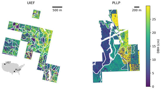
Figure 1.
Spatial distribution of trees, symbolized by DBH, across forest stands within the UIEF (left) and PLLP (right) study areas.
The PLLP Digital Inventory® used in this study is located in Bienville Parish, southwest of Bienville, LA, USA (Figure 1, right pane). The dataset was collected from a 270 (670-acre) even-aged commercial conifer plantation. A private landowner, participating in a multi-state 600,000 ALS-based forest inventory, offered our team access to this stand. The elevation of these stands was 100 above sea level, the soil composition was a well-drained upland Betis loam and the topography exhibited a slight west-facing aspect. The local climate is characterized by mild winters and hot, humid summers. The mean summer (June–August) temperature over the 1991–2020 period was , the mean summer precipitation was 95 , and the mean annual precipitation was 117 [34]. The subject stands were established in 1995 as a single-species plantation and were commercially thinned to remove every 5th row prior to field measurement.
2.2. ALS Data and Preprocessing
The ALS data for the UIEF study area were acquired in July 2022 using a RIEGL VQ-1560II sensor (RIEGL, Horn, Austria) mounted on a fixed-wing aircraft fitted with a Gyro Stabilization Mount (SOMAG, Jena, Germany). The elevation of the aircraft was maintained between 2000 and 2500 above ground level, and flight lines alternated orientations while maintaining a 50% flight-line overlap with respect to the 58 sensor field-of-view. The average scan density was 22 pulses per square meter with an average per-pulse return rate of four over forested landscapes. The ALS data were preprocessed to normalize laser intensity within the RIEGL RiPROCESS software v. 1.9.2.4 (RIEGL, Horn, Austria) and classified to bare earth, vegetation, water, buildings, and noise returns before being tiled into 500 . LAZ file-type tiles by the LiDAR acquisition company (Airborne Imaging, Calgary, AB, Canada).
ALS data for the Louisiana study area were acquired in December 2020 using a RIEGL VQ-1560II sensor (RIEGL, Horn, Austria) mounted on a fixed-wing aircraft fitted with a Gyro Stabilization 4000 Mount (SOMAG, Jena, Germany). Elevation of the aircraft was maintained between 1600 and 1900 above ground level and flight lines alternated orientations while maintaining a 50% flight-line overlap with respect to the 58 sensor field of view. The average scan density was 20 pulses per square meter with an average pulse return rate of four. The ALS data were preprocessed to normalize laser intensity within the RIEGL RiPROCESS software (RIEGL, Horn, Austria) and classified to bare earth, vegetation, water, buildings, and noise returns before being tiled into 500 .LAZ file-type tiles by the LiDAR acquisition company and delivered to our team.
2.3. ALS Individual Tree Detection and Measurement
The ALS .LAZ files were imported into ForestView® for individual tree detection and the processing of stand- and individual tree-metrics. Individual tree detection within this software begins with the generation of a digital elevation model (DEM) and digital surface model (DSM) in order to generate a canopy height model (CHM) at resolution directly from the ALS point cloud. The software then iterates through multiple methods, similar to watershed and local maxima algorithms [35,36,37], that detect peaks in the CHM. These peaks are assumed to be the tops of tree “approximate” objects; thus, their location and respective height are recorded. For tree-attribute estimation, the software relies on an internal database of field- and ALS-measured stem-mapped trees, each having diameter at breast height (DBH), height, species, crown condition, and taper information. The software calculates a large number (100+) of metrics from the ALS point cloud for each individual tree object and uses these metrics along with the field-measured attributes in the database to model tree attributes for each ALS-detected tree. The DBH modeling draws on height-, crown-, density-, and spacing-related metrics derived from the ALS point cloud data and their respective allometric relationships to the trees stem mapped in the field. Further details on ForestView® processing and outputs are reported in [30]. The individual tree location, maximum height, and DBH were the only ForestView® derived Digital Inventory® metrics utilized in this research. Additional outputs available but not assessed in this study were various crown descriptors, height to live crown, social dominance, and gross stem volume.
2.4. Digital Inventories
This simulation study uses two datasets consisting of a subset of the UIEF stands and PLLP stands that provide a realistic representation of a natural forest, where the spatial distribution of trees and their sizes are influenced by a complex interplay of ecological and environmental factors.
The UIEF dataset represents 99,420 trees from 85 stands. The average stand size is approximately ∼5 (∼12 acres) (Figure 1, left panel). The inventory includes stands of varying sizes and tree compositions. Douglas fir is the most prevalent species, comprising 49% of the total. This is followed, in descending order, by western redcedar, ponderosa pine, lodgepole pine, and western larch, with grand fir being the least represented species, accounting for only 1% (see Figure 2). The distribution of heights and diameter at breast height (DBH) exhibits a bimodal pattern, with DBH peaks around 40 (∼16 inches) and 13 (∼5 inches), and height peaks at approximately 30 and 10 (see Figure 3 upper pane). Figure 4 shows the spatial distribution of TPA and BAA for the stands in each study area. While there is a slight positive correlation between these two metrics, the relationship is not strongly linear. Some stands have a high tree density while maintaining a median BAA and vice versa. The average TPA is 107 and the average BAA is 100.
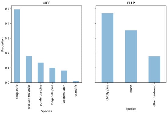
Figure 2.
The distribution of the species in the selected UIEF (left) and PLLP (right) stands.
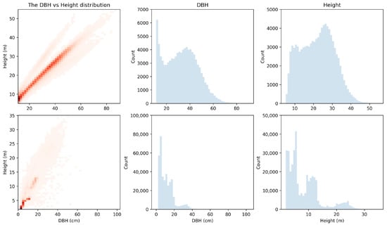
Figure 3.
Tree height and DBH distributions, along with the observed height–diameter relationship of the selected UIEF (top) and PLLP (bottom) stands.
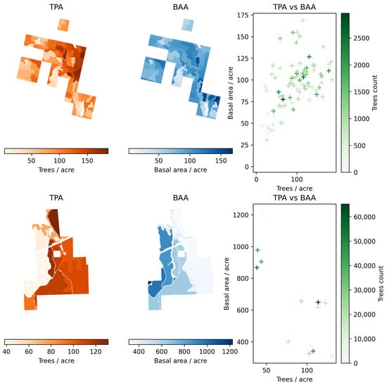
Figure 4.
Basal area per acre (BAA) and trees per acre (TPA) aggregated at the stand level across the UIEF (top) and PLLP (bottom) study area.
The PLLP dataset included 18 stands and 372,773 trees. The average stand area was 15 (36 acres), which led to all stands being of greater size and more dense compared to the UIEF. The distribution of heights and diameter at breast height (DBH) (see Figure 2 right panel) shows that the majority of trees were concentrated at small sizes. The DBH peaks sharply around (∼3 inches) with a secondary, less pronounced mode near (∼8 inches). Heights display a dominant peak at approximately 5 with smaller clusters extending toward 10 to 15 and a third cluster at 25 . The overall structure indicates a younger or more densely regenerated stand characterized by a large number of small-diameter, shorter trees with an average TPA of 91 and an average BAA of 567.
The ALS and field measurements for the UIEF and the PLLP were completed following the same protocols to maintain as much consistency as possible for analysis purposes. The final inventory was built using ForestView®, which is a gray box tree detection and measurement algorithm that is described in detail in [30,31]. The ForestView® Digital Inventory® product is a full population estimate of the forest with a spatially registered tree list and attributes that serve as the baseline for this study. The authors acknowledge that the Digital Inventory® used as the baseline for this study is an estimate and may be statistically biased in relation to the true forest in various aspects. However, the individual-tree dataset provides a reasonable representation of forest structure and distribution that eliminates the need to simulate many configurations of complex forest structures seen in the western and southeastern United States.
2.5. Sampling Simulation
With the Digital Inventory® representing the total forest population, we defined 107 forest inventory cruise alternatives (see Appendix A.2) that varied in noise levels, error rates, sampling schemes, and edge plot methodologies. The simulated cruise specification consists of 8 parameters (see Table 1) including the VRP specifications, plot selection parameters, and parameters defining some potential sources of errors (noise simulation). The sampling simulation was coded in a combination of Rust v. 1.89.0 [38] and Python v. 3.12 [39] to apply a set of cruise specifications to the Digital Inventory® to retrieve a sampled tree list.

Table 1.
The parameters used in the sampling simulation VRP experiments and their default values.
Each cruise was applied to the digital inventory 10,000 times, and the sample mean and variance of key forest metrics (i.e., tree count and basal area) were calculated for each simulation. We then evaluated the accuracy and reliability of the simulated sample-derived estimates by comparing them to the corresponding true population means for each metric (see Figure 5).
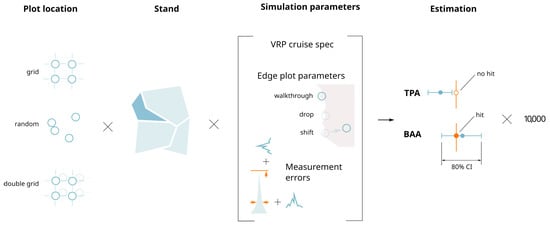
Figure 5.
Structure of the simulation experiment. The simulation is conducted for each plot location method across all stands. For every combination of stand and simulation parameters, forest metrics are estimated, confidence intervals are derived, and the inclusion (hit) or exclusion (no hit) of the true population mean is evaluated. Each combination is repeated 10,000 times.
The edge plot methods used in the simulations are described below. Parameters controlling the simulated measurement errors are documented in Appendix A.1.
- Drop: This drops an edge plot from all calculations and only uses plots that are not identified as edge plots as determined by a buffer distance from the stand boundary.
- Shift: This moves an “edge plot” to the nearest point within a negatively buffered stand polygon as determined by a buffer distance from the stand boundary.
- Walkthrough: This cruises an edge plot using the walkthrough method as it was described in Ducey et al., 2004 [40] where a tree is double counted if the stand boundary is closer to the tree than the plot center is to the tree along the same azimuth from the plot center.
The entire space of possible parameter combinations was not exhaustively explored. Instead, testing was limited to a subset of reasonable and practical combinations. Most experiments were conducted by holding all parameters at their default values (Table 1) and varying only one parameter at a time (see Appendix A.2 for a full list).
This experiment was repeated several times for different plot location schemes (see Figure 6b) with the UIEF including three methods (grid, random, double grid) and the PLLP including two methods (grid and random):
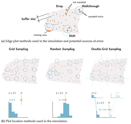
Figure 6.
Visualization of field plot sampling methods used in the simulation. (a) Edge plot methods: the Drop method excludes plots within a buffer distance of the stand boundary, which can lead to missing trees near edges; the Shift method relocates edge plots inward, potentially omitting trees that would otherwise be sampled; and the Walkthrough method (after Ducey et al., 2004 [40]) samples certain trees twice. The buffer size determines the width of the edge zone; when set too small, plots not technically on the boundary may still have unmeasured areas. (b) Plot location methods: the grid sampling method assigns plots on a grid with a random offset of less than one grid spacing, which can cause systematic over- or under-sampling depending on systematic patterns of spatial tree distribution; the random sampling method places plots uniformly at random within the stand; and the double-grid method overlays two independent grids (after Freese, 1962 [9]), producing two random and statistically independent estimates per stand, from which the final estimates and confidence intervals are derived.
- Grid Sampling: Plots are assigned on a grid with a uniform random shift less than the grid spacing applied to the grid origin for each simulation and stand sample,
- Random Sampling: Random plot locations are assigned within the stand boundary at the target grid density
- Double grid: Each stand is overlaid with two grids, with the origin point of each grid selected at random, as described by Freese 1962 [9], which results in two independent estimations for a single stand. Since the two estimations are derived randomly and independently, they can be treated as truly random values. The final estimate and its confidence interval are then calculated based on these two values.
The simulations were also repeated on the UIEF inventory using random stands, described as follows, to quantify how improper stand delineation affects inventory outcomes. In this case, “artificial” stands were created by constructing Voronoi polygons from uniformly distributed seed points across the study area. This design provides a neutral framework for testing the sensitivity of stratified estimators to boundary mis-specification. The Voronoi polygons in Figure 7 represent artificial stand delineations derived from uniformly distributed seed points across the landscape.
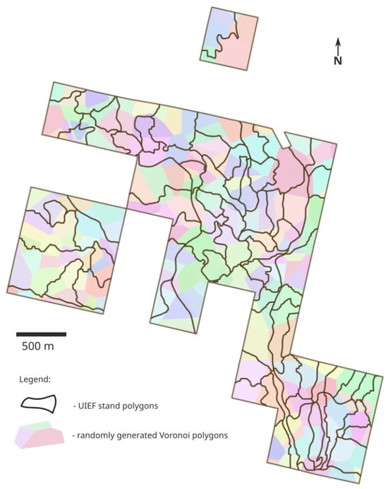
Figure 7.
The UIEF stand boundaries (solid black lines) overlaid on randomly generated Voronoi polygons (colored regions) used in the experimental stratification.
The total number of simulations for the UIEF—107 cruise specifications for 85 stands with 10,000 simulations for every spec–stand combination was 90,950,000 simulations per plot location method. The total number of simulations for the PLLP—87 cruise specifications for 18 stands with 10,000 simulations for every spec–stand combination—was 15,660,000 simulations per plot location method.
2.6. Analysis
Each simulation produces a sampled tree list for every plot within each stand. The plot data are compiled to estimate the mean tree count, basal area, and volume (as basal area times height) per acre at each plot location. The statistical mean and variance across the plots are then recorded for each stand. We can report that a confidence interval for each stand is typically calculated from the theoretical uncertainty of the sample using the standard error of the plot level mean estimates [41] as
where is the sample mean, is the critical value from the t-distribution with degrees of freedom at the desired confidence level , s is the sample standard deviation, and n is the number of plots.
A confidence level of 95% is widely used across industries, especially those with ample data and more clearly defined trends (e.g., medical, insurance, finance, etc.) [42]. However, in complex and highly variable forest structures, often paired with reduced sample sizes, high confidence levels can lead to very large and potentially nugatory confidence intervals [43]. Additionally, higher confidence levels require more sample plots [44], increasing the cost of forest inventory efforts. Therefore, it is common for industrial forest landowners to use a confidence level less than 95% (e.g., 90% or 80%) for standard forest metrics such as volume per acre, BAA, or TPA if the inventory project allows. This tightens upper and lower bounds while maintaining adequate confidence that the true mean lies within the interval [27,45]. This is not always ideal or possible when considering the more rigorous tolerances of some inventory projects such as forest carbon offset quantifications or land transaction valuations [46,47]. In this study, we assessed the reliability of the confidence intervals (CIs) produced by each plot selection method. For each stand in each simulation, we calculated an 80% confidence interval and evaluated whether it captured the true mean of the LiDAR-based population of the stand. This process was repeated across 10,000 simulations per stand. The proportion of simulations in which the true value fell within the estimated CI (i.e., estimate ± CI) was recorded as the hit rate. In theory, this hit rate should align with the nominal confidence level—meaning approximately 80% of the intervals should contain the true mean of the stand.
For this research, we used the simple mean and simple estimation for the variance that is most widely used within the practice of building inventories. There are estimators that are potentially more suitable for the task of estimating the variation around the mean and spatial autocorrelation more adequately [23,28].
To evaluate the performance of different sampling schemes, we assessed both the accuracy and the uncertainty of the simulated estimates. Accuracy was quantified using normalized bias, which was defined as the mean bias from the true population mean of all simulations for a given stand and field specification divided by the true mean. Normalization allowed a direct comparison of bias across stands and attributes with different magnitudes.
Uncertainty was evaluated through the empirical coverage of nominal CIs. For each simulation, 80% CIs were constructed for the number of trees per acre (TPA) and the basal area per acre (BAA). The empirical hit rate—the proportion of simulations in which the CI contained the true mean—was then compared against the nominal 80% expectation. Deviations from the nominal level indicate either under-coverage (intervals too narrow) or over-coverage (intervals too wide).
Together, these metrics provide a basis for assessing both the calibration and reliability of different sampling schemes.
3. Results
Figure 8 and Figure 9 present the results of simulated TPA and BAA sample estimates for the UIEF and PLLP stands for all simulations by plotting the empirical hit rate against the normalized bias. The figure reveals the miscalibration of the 80% confidence intervals (CIs) for the systematic grids. The graphs reveal that many simulations failed to achieve the nominal 80% hit rate, especially in cases where the normalized bias deviated substantially from zero. A general tendency toward negative bias is observed, meaning that estimates frequently fell below the true values. Interestingly, basal area estimates exhibit a pattern of coverage rates exceeding the nominal 80% level (over-coverage)—suggesting that the intervals for this variable may be overly conservative in the statistical sense, i.e., being wider than necessary to achieve the nominal coverage probability.
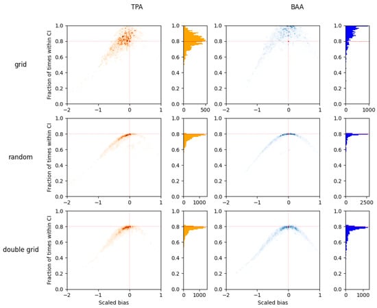
Figure 8.
Results for the simulations on UIEF dataset: Density maps showing the hit rates of 80% confidence intervals for all simulated systematic VRP cruises using different plot location methods. Red lines indicate the theoretically expected hit rate (80%) and zero bias. Each data point on the graph represents a summary for 10,000 simulations for a pair of stand and cruise specifications for the many simulated cruises across the study area. The scatter distributions and marginal histograms reveal substantial over-coverage for grid-based plot locations, where the observed hit rates averaged ∼85% for TPA and ∼95% for BAA compared to the nominal 80%.
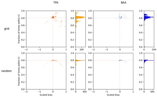
Figure 9.
Results for the simulations on the PLLP dataset: density maps showing the hit rates of 80% confidence intervals for all simulated systematic VRP cruises using different plot location methods. Red lines indicate the theoretically expected hit rate (80%) and zero bias. Each data point on the graph represents a summary for 10,000 simulations for a pair of stand and cruise specifications of the many simulated cruises across the study area. The shape of the scatter and the histogram suggest a significant over-coverage and incorrectly estimated CI for the simulations that used plots located on a grid.
Table 2 summarizes the median normalized bias across different plot location schemes. For both TPA and BAA, the grid, random, and double-grid placement produced very similar levels of bias with values generally below ±0.2. In contrast, the random placement within incorrectly stratified stands produced a markedly higher bias for BAA.
Table 2.
Median normalized bias for different plot location schemes aggregated across combinations of field cruise specification and stands. Normalized bias is presented as a dimensionless ratio, which is calculated as the difference between estimated and true values divided by the confidence interval. Values closer to zero indicate less bias relative to the uncertainty of the estimate.
Figure 10 and Figure 11 show a simplified summary of the distribution of hit rates across different plot layout methodologies (grid, random, and double grid) for the UIEF and PLLP study areas. For both study areas, the gridded method shows the widest range of simulated hit rates, indicating that it was the least effective method for reliably estimating an accurate confidence interval. The distribution of hit rates for the estimates using the “double grid” plot location method yielded results comparable to those obtained using the random plot location method. Even though the random plot location method yielded more accurate estimations for the CI out of the three methods used (Figure 12)—the negative bias is still evident. For the UIEF, the using “walkthrough”-only specifications (marked with an asterisk in the figures) consistently improved the hit rates relative to their mixed-method counterparts, highlighting the influence of edge plot handling. In contrast, no such improvement was observed for the PLLP.
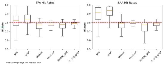
Figure 10.
The hit rates of 80% confidence intervals for all simulated systematic VRP cruises on the UIEF using different plot location methods. Red lines indicate the theoretically expected hit rate (80%). The random and “double-grid” methods show the results closer to those theoretically expected. Names marked with an asterisk (*) indicate cases where only the “walkthrough” edge plot method was used, which generally improved the hit rate for random and double-grid methods.
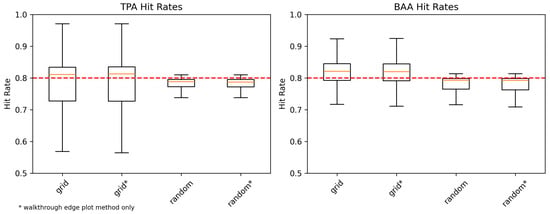
Figure 11.
The hit rates of 80% confidence intervals for all simulated systematic VRP cruises on the PLLP using different plot location methods. Red lines indicate the theoretically expected hit rate (80%). The random plot location method show the results closer to those theoretically expected. Names marked with an asterisk (*) indicate cases where only the “walkthrough” edge plot method was used, which shows no improvement for the PLLP stands.
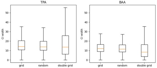
Figure 12.
The distribution of confidence interval width for the simulated samples using different plot placement methods for the UIEF. The double-grid method shows more variance in the CI estimations.
4. Discussion
The simulation results present multiple findings that confirm previous contributions from the existing literature around sample design and provide new insights in the context of modern forest measurement technology within the following categories:
- Definition of stands as the sampling target;
- Spatial sampling scheme of plots within a stand including stand edge methodology;
- Plot measurement specification.
We are also aware of additional potential sources of error that are overlooked in the handling of traditional inventory methodologies; these were considered outside the scope of this study but warrant additional investigation.
4.1. Definition of Stands as the Sampling Target
Forest managers must pay careful attention to the sample design of an inventory because an appropriate stratification is critical with respect to sampling for, and the estimation of, precision and accuracy [4]. Stratification—dividing heterogeneous populations into internally homogeneous units—minimizes within-stratum variability and maximizes between-stratum variance, resulting in more precise estimates for a given sample size [48,49]. In practical field inventories, this typically translates into delineating forest stands by attributes such as species composition, age class, canopy density, or site productivity [50]. Effective stand delineation not only reduces variance from sampling methodologies but also contributes to improved logistical efficiency, often reducing the number of sample plots necessary to meet a desired level of statistical sampling accuracy [27,51]. However, stand delineation is inherently subjective—boundaries are often drawn based on imperfect remote-sensing interpretation, field reconnaissance, or silvicultural definitions.
Misclassification or improperly drawn boundaries can introduce stratification bias, undermining estimator accuracy even when standard stratified sampling formulas are applied. For example, the results presented in Table 2 show that the improperly delineated stands introduce a significant bias in the final estimation of the BAA (with a 0.23 normalized bias). Furthermore, throughout the forestry business sector, it is widely known that the stand boundaries used for forest inventory and silviculture purposes rarely overlap with the boundaries used for timber harvest operations. As such, the quality of an existing stand layer available to a given forest manager for inventory sampling design is likely to vary significantly, and the creation of a new stand layer is often a time-intensive effort. We acknowledge that the alternate delineation methodology employed in this study represents a likely “worst-case” scenario for this forest structure, but it provides initial context for further investigation regarding a source of error typically ignored in confidence interval estimations.
4.2. Spatial Design of a Stand Sample
Common traditional inventory practices use statistical estimators that assume the underlying sample is taken randomly from a normal distribution; in many ways, natural forest configurations and the most frequently used sampling techniques independently violate these assumptions. Although forest managers make their best effort to group the population of trees being sampled into homogeneous stands, the spatial distribution of tree locations must follow certain physical constraints. Constraints such as the minimum spacing and distributions of tree diameter and height tend to follow log-normal distributions. Both of these forest structural attributes are in conflict with the statistical assumptions used for estimators commonly relied on by forest managers.
For example, generally, the stand structure is governed by factors such as species composition, stand age, competition, and site conditions, all of which vary across the landscape. The relationships among these factors within a stand are rarely linear, reflecting the inherent variability and complexity of forest ecosystems. Häbel et al. (2019) [52] showed that the plot size plays a significant role depending on how clustered the forest is. Nonlinear stand density indices can introduce bias and uncertainty, which vary with the sample size and variance–covariance structure of measured variables [53]. Specifically, the DBH values within each stand are not randomly distributed but instead represent a mixture of several log-normal distributions, reflecting the natural variation in tree sizes. The basal area factor (BAF) and plot size influence the precision and accuracy of forest inventory estimates with coefficients of variation decreasing as the plot size increases and BAF decreases [54]. These deviations from the assumptions of randomness likely contribute to the observed bias in simulations and the incorrect CI estimations. Understanding these factors can help optimize forest inventory design, potentially improving precision or reducing costs [52].
In some cases, especially when the TPA or BAA of a stand is low and sparse, the distribution of resulting samples does not follow a normal distribution. This tends to cause the lower bound estimate of a reported confidence interval around the mean to be lower than expected (see marginal histograms on Figure 8 and Figure 9). Furthermore, in these non-normal examples, the expected value of the sample falls close to the true mean, but the “most likely” or median occurrences from an individual sample will often underestimate the true population mean. These concepts are difficult to translate into meaningful insights for forest managers, but they do highlight the importance and challenges of accurately capturing and estimating the uncertainty caused by spatial variability in a sample-based cruise.
The largest contributor to poorly calibrated hit rates is the methodology used for plot layout. As shown in our study (Figure 8 and Figure 9), the random plot placement more reliably estimates CIs for TPA and BAA. Historically, the gridded plot layout has been strongly favored over the random layout due to the in-field operational efficiencies associated with collections on a systematic grid. Given the advances in mobile GPS and collection technologies over previous decades, it may be worth reconsidering the operational and statistical trade-offs presented by gridded plot layouts. Another alternative is the double-grid method, which requires only modestly greater effort than a single grid while producing results that closely approximate those of random sampling. However, a negative bias remains evident with a strong correlation between this bias and the lower hit rates in the simulations with random plot placement and the double grid (Table 2). This suggests that while better plot placement addresses some issues, other factors contributing to the bias may still need to be considered.
The estimations of the BAA had less absolute normalized bias (<0.1) for both UIEF and PLLP, while the estimations of the TPA for the UIEF had an average absolute normalized bias around (0.15). Additionally, as shown in Figure 12, the final estimates are less precise—the distribution of confidence intervals shows more variance in confidence intervals, which is expected given that the estimation is based on only two data points. However, Hill et al. (2018) [55] showed that a double-sampling extension to the German National Forest Inventory reduced variance by 25%–43% compared to simple random sampling.
Another option to address the observed biases and variability in hit rates is to use a more sophisticated estimator that accounts for the non-randomness in tree distributions and sampling (e.g., [23,28]), although such approaches typically require additional information on the precise plot location, spatial tree distributions, assumptions about underlying stand structure, or more complex computational procedures.
Magnussen et al. (2020) [28] found that alternatives to the simple random sampling (SRS) estimator performed better, especially in populations with spatial autocorrelation. Reber and Ek (1983) [56] demonstrated that systematic samples with multiple random starts provided variance estimates comparable to cluster sampling in Minnesota timber stands. However, Whysong and Miller (1987) [57] reported that systematic plot placement was significantly affected by clumping and pattern intensity, while random sampling produced more consistent frequency estimates.
The results in Table 2 emphasize that one of the greatest sources of potential bias is the edge method chosen for data collection. When all edge methods, with the exception of the walkthrough method, are removed from the simulation, the result is a reduction in normalized bias from −0.16 to −0.10 for TPA and from −0.08 to 0.00 for the BAA for the UIEF stands. This is consistent with findings from previous studies [29,58,59,60,61], which showed that edge methods strongly influence the accuracy of forest inventory estimates. The activity of dropping plots or shifting plots inside a forest stand for sampling tends to produce further biased results than more simplistic methods such as a “walkthrough” [40]. Furthermore, using a boundary buffer for “edge plot” selection for drop and/or shift methods produces further increases in bias and skews results.
Overall, the results of this study are broadly consistent with those of Gordon and Pont (2015) [29], who similarly reported that grid sampling, or single-point sampling, introduced a bias and resulted in unreliable confidence intervals. While in their study VRP cruises were not simulated, their results also suggest that both the choice of sampling design and the accuracy of stand boundaries play critical roles in ensuring unbiased estimates. It is worth mentioning that Gordon and Pont (2015) [29] examined only four stands dominated by a single species (Pinus radiata pine), in a New Zealand context, using a LiDAR dataset of different specifications, whereas our analysis covers a significantly larger number of stands with greater species diversity and broader geographic representation.
4.3. Tree Selection and Measurement
Our observation that many of the plot-level VRP cruise specifications (BAF, BAF_DBH, Fixed plot radius) did not significantly impact the bias of the final estimation in comparison to plot layout and edge plot methods was informative. Because most sampling methods produced little bias in stand-level estimates, and when the inefficient edge plot methods (drop, shift) are excluded, the remaining bias is minimal. Under these conditions, the primary difference among simulations lies in the mean estimation of variance, which tends to increase as the BAF multiplier grows. In particular, the highest variance occurs when the BAF used in the cruise was poorly matched to the actual stand conditions, highlighting that variance inflation rather than systematic bias is the main risk associated with suboptimal BAF selection.
4.4. Unexplored Sources of Error That Require Further Investigation
Although this study is one of the most comprehensive studies of its kind to date, we have still only covered a subset of possible forest configurations, species types, and potential sources of error. Future studies incorporating a greater diversity of forest types, stand configurations, and successfully matched silvicultural stand boundaries with operational harvest boundaries may provide additional insights that increase our collective understanding and use of population-level forestland inventories.
Another potential source of variance that requires further study is the statistical effect of modeling techniques used when only a limited number of tree heights are measured. It is likely that the calculated variance would underestimate the true variance of a population due to a “reversion to the mean” phenomenon that reduces variance within a modeled population [62]. However, the population data applied in this study use modeled DBH values, making this more difficult to accurately quantify. Furthermore, the results of this research approach may vary by forest type, geography and tree type (i.e., deciduous forest vs. conifer) with respect to the variance observations of diameter and height.
Lastly, further simulation and a more detailed assessment would be beneficial to further quantify the potential magnitude of bias introduced by incorrect groupings of trees to stands and stands to strata. A “worst-case” example of improper stand delineation was shown in this study (see Table 2), demonstrating the influence that stand boundaries may have on the resultant forest inventory. Traditional forestry often groups stands by strata and only samples a subset of stands to inform a pooled variance approach. Because these strata typically rely on a priori information about individual stand strata, future research should consider this as another possible source of bias within sampling methodologies.
4.5. Opportunities from Wall-to-Wall Remote Sensing Data
The current study was based on a complete forest inventory derived from ALS data. As demonstrated, replicating such a full-coverage inventory using conventional plot-based methods presents several challenges. Wall-to-wall remote sensing data—particularly ALS and other high-resolution spatial data—offer potentially significant methodological advantages. These population-level datasets offer enhanced presampling stratification opportunities that may mitigate several weaknesses of traditional sampling, including the need for strict stand delineation and manual edge corrections [63]. Furthermore, the existence of a population-level inventory would facilitate a more refined stratification, leading to increased efficiencies and accuracies for regional-scale inferences [64,65,66]. The inclusion of wall-to-wall spatial datasets within forestry offers a potential shift toward more robust and scalable forest sampling, inventory, and monitoring systems [17,21,67,68].
5. Conclusions
Traditional sampling-based approaches in forest inventory, which rely on the systematic or stratified random sampling of field plots, have long served as the cornerstone for estimating key forest attributes at the stand or landscape level. However, these methods are not without limitations. This study demonstrates that while standard cruise specifications such as BAF, BAF_DBH, and fixed-radius plots do not introduce systematic bias, the design and implementation of plot placement and edge methods play a decisive role in both the accuracy and precision of forest inventory estimates. Random plot placement produced the most reliable confidence intervals compared to a population for TPA and BAA, though the greater field cost limits this method’s operational feasibility. A double-grid design offered a practical compromise, closely approximating the random sampling method results with only modestly greater effort than a single grid, though a small negative bias remained compared to the population. This research provides greater clarity around the influence of edge methods and stand delineations, demonstrating that the choices made by practitioners carry the most significant sources of error for BAA estimates (0.23 normalized bias for incorrectly delineated stands and no bias when using only the walkthrough edge plot method for the UIEF inventory). Taken together, the findings underscore the importance of sampling design decisions beyond the choice of plot size or BAF particularly when inventories are scaled across heterogeneous landscapes. The inclusion of wall-to-wall spatial datasets within forestry offers a potential shift toward more robust and scalable forest sampling, inventory, and monitoring systems [17,21,67,68].
Author Contributions
Conceptualization: M.V.C.; methodology: M.V.C. and A.M.S.S.; software: M.K.; validation: M.V.C., R.A. and A.M.S.S.; formal analysis: M.K. and R.A.; investigation, data resources and data curation: M.V.C. and R.A.; writing—original draft preparation: M.K.; writing—review and editing: M.V.C., R.A. and A.M.S.S.; visualization: M.K.; supervision and project administration: M.V.C. All authors have read and agreed to the published version of the manuscript.
Funding
This research received no external funding.
Data Availability Statement
The data are available within the article.
Acknowledgments
We would like to thank biometricians Logan Wimme, Michael M. Huebschmann and Steve N. Scharosch for their review and comments on field specifications. We would also like to thank A. Sparks for their general review and comments on the paper. During the preparation of this manuscript, the authors used ChatGPT version 4 for the purposes of providing some early outline structure and for some minor grammar corrections at later stages. The authors have reviewed and edited the output and take full responsibility for the content of this publication. Data collection, experiment design, development of the paper, and figures were all completed by the research team with no assistance from AI.
Conflicts of Interest
M.V. Corrao and R. Armstrong are employed by Northwest Management Incorporated. The remaining authors declare that the research was conducted in the absence of any commercial or financial relationships that could be construed as a potential conflict of interest.
Abbreviations
The following abbreviations are used in this manuscript:
| ALS | Airborne laser scanning |
| BAA | Basal area per acre |
| BAF | Basal area factor |
| CI | Confidence interval |
| CFI | Continuous forest inventory |
| CHM | Canopy height model |
| DEM | Digital elevation model |
| FIA | Forest inventory and analysis |
| LiDAR | Light detection and ranging |
| PLLP | Single-species plantation of Pinus taeda (Loblolly pine) |
| RMSE | Root mean square error |
| TPA | Trees per acre |
| VRP | Variable radius plot |
| UIEF | University of Idaho Experimental Forest |
Appendix A
Appendix A.1. Parameters Controlling Measurement Error
The parameters controlling some potential measurement errors were included to simulate realistic sources of errors during the field cruises.
- Basal area factor (BAF) multiplier: To mimic a realistic cruise, the optimal BAF to achieve a tally of 10 trees per plot is estimated for each stand. To determine this optimal BAF, a single simulation is performed for each stand using the specification with the default BAF to establish a baseline tally. Then, a grid search is conducted over a range of possible BAF values, running simulations for each candidate value to estimate the average number of tallied trees per plot. After that, a multiplier is applied to the optimal BAF to approximate a cruiser systematically using a larger or smaller BAF.
- DBH noise error: This is a magnitude of the noise added to the DBH measurements in inches where 0.0 means no measurement errors, 2.0 means a random noise centered around 0 and with sigma equal to 2.0 inches is added to each measurement.
- Height noise error: This is a scale of the normally distributed noise that is added to the height measurements. 0.0 means that no errors will be added, while 0.01 means that for every height measurement, the normally distributed error will be added with the sigma equal to 1% of the height.
Appendix A.2. Field VRP Specifications Used for the Simulations
The inverse of plot area is reported in imperial units () to maintain consistency with the standard field protocols and sampling design used in U.S. forestry practice, which this study aims to replicate.
The simulations were conducted by varying one parameter at a time and holding other parameters constant at their default values (see Table 1):
- 1.
- Variable DBH noise:
- Inverse of plot area, : 10;
- DBH Noise (Error), cm: 0.0, 1.25, 2.5, 3.75, 5.0, 6.25.
- 2.
- Variable height noise:
- Inverse of plot area, : 10;
- Height Noise (Error), m: 0.0, 0.5, 1.0, 1.5, 2.0, 2.5.
- 3.
- Variable BAF multipliers:
- Inverse of plot area, : 10;
- BAF DBH: 10;
- BAF multipliers: 0.5, 0.75, 1, 1.5, 2, 3.
- 4.
- Variable Fixed Sub-Plot Radius:
- Inverse of plot area, : 5, 7.5, 10, 12.5, 15, 17.5, 20, 22.5, 25, 27.5, 30.
- 5.
- Variable grid spacing (plot density):
- Grid Spacing, m: 70, 72.5, 75, 77.5, 80, 82.5, 85, 87.5, 90, 92.5, 95, 97.5.
- 6.
- Variable buffer with “shift inside” edge plot method:
- Method: “shift inside”;
- Buffer, m: 0, 2.5, 5, 7.5, 10, 12.5, 15, 17.5, 20, 22.5.
- 7.
- Variable buffer with “walkthrough” edge plot method:
- Method: “walkthrough”;
- Buffer, m: 0, 2.5, 5, 7.5, 10, 12.5, 15, 17.5, 20, 22.5, 25, 27.5, 30, 32.5.
- 8.
- Variable buffer with “drop” edge plot method:
- Method: “drop”;
- Buffer, m: 0, 2.5, 5, 7.5, 10, 12.5, 15, 17.5, 20, 22.5, 25.
The full list of simulations:
Table A1.
Parameters used for the VRP cruise simulation.
Table A1.
Parameters used for the VRP cruise simulation.
| Spec_ID | Baf_Dbh | Baf Multiplier | Area Inv_Acres | Grid Spacings | Noise Errors | Height_Noise Errors | Buffer | Edge_Plot Method |
|---|---|---|---|---|---|---|---|---|
| 0 | 5 | 1 | 10 | 80 | 0 | 0 | −20 | walkthrough |
| 1 | 5 | 1 | 10 | 80 | 0.5 | 0.5 | −20 | walkthrough |
| 2 | 5 | 1 | 10 | 80 | 1 | 1 | −20 | walkthrough |
| 3 | 5 | 1 | 10 | 80 | 1.5 | 1.5 | −20 | walkthrough |
| 4 | 5 | 1 | 10 | 80 | 2 | 2 | −20 | walkthrough |
| 5 | 5 | 1 | 10 | 80 | 2.5 | 2.5 | −20 | walkthrough |
| 6 | 5 | 1 | 10 | 80 | 0 | 0 | −20 | walkthrough |
| 7 | 5 | 1 | 10 | 80 | 0 | 0.5 | −20 | walkthrough |
| 8 | 5 | 1 | 10 | 80 | 0 | 1 | −20 | walkthrough |
| 9 | 5 | 1 | 10 | 80 | 0 | 1.5 | −20 | walkthrough |
| 10 | 5 | 1 | 10 | 80 | 0 | 2 | −20 | walkthrough |
| 11 | 5 | 1 | 10 | 80 | 0 | 2.5 | −20 | walkthrough |
| 12 | 5 | 1 | 10 | 80 | 0 | 0 | −20 | walkthrough |
| 13 | 5 | 1 | 10 | 80 | 0.5 | 0 | −20 | walkthrough |
| 14 | 5 | 1 | 10 | 80 | 1 | 0 | −20 | walkthrough |
| 15 | 5 | 1 | 10 | 80 | 1.5 | 0 | −20 | walkthrough |
| 16 | 5 | 1 | 10 | 80 | 2 | 0 | −20 | walkthrough |
| 17 | 5 | 1 | 10 | 80 | 2.5 | 0 | −20 | walkthrough |
| 18 | 5 | 0.5 | 10 | 80 | 0 | 0 | −20 | walkthrough |
| 19 | 5 | 0.75 | 10 | 80 | 0 | 0 | −20 | walkthrough |
| 20 | 5 | 1 | 10 | 80 | 0 | 0 | −20 | walkthrough |
| 21 | 5 | 1.2 | 10 | 80 | 0 | 0 | −20 | walkthrough |
| 22 | 5 | 1.5 | 10 | 80 | 0 | 0 | −20 | walkthrough |
| 23 | 5 | 2 | 10 | 80 | 0 | 0 | −20 | walkthrough |
| 24 | 5 | 3 | 10 | 80 | 0 | 0 | −20 | walkthrough |
| 25 | 5 | 1 | 5 | 80 | 0 | 0 | −20 | walkthrough |
| 26 | 5 | 1 | 7.5 | 80 | 0 | 0 | −20 | walkthrough |
| 27 | 5 | 1 | 10 | 80 | 0 | 0 | −20 | walkthrough |
| 28 | 5 | 1 | 12.5 | 80 | 0 | 0 | −20 | walkthrough |
| 29 | 5 | 1 | 15 | 80 | 0 | 0 | −20 | walkthrough |
| 30 | 5 | 1 | 17.5 | 80 | 0 | 0 | −20 | walkthrough |
| 31 | 5 | 1 | 20 | 80 | 0 | 0 | −20 | walkthrough |
| 32 | 5 | 1 | 22.5 | 80 | 0 | 0 | −20 | walkthrough |
| 33 | 5 | 1 | 25 | 80 | 0 | 0 | −20 | walkthrough |
| 34 | 5 | 1 | 27.5 | 80 | 0 | 0 | −20 | walkthrough |
| 35 | 5 | 1 | 30 | 80 | 0 | 0 | −20 | walkthrough |
| 36 | 5 | 1 | 20 | 70 | 0 | 0 | 0 | shiftinside |
| 37 | 5 | 1 | 20 | 72.5 | 0 | 0 | 0 | shiftinside |
| 38 | 5 | 1 | 20 | 75 | 0 | 0 | 0 | shiftinside |
| 39 | 5 | 1 | 20 | 77.5 | 0 | 0 | 0 | shiftinside |
| 40 | 5 | 1 | 20 | 80 | 0 | 0 | 0 | shiftinside |
| 41 | 5 | 1 | 20 | 82.5 | 0 | 0 | 0 | shiftinside |
| 42 | 5 | 1 | 20 | 85 | 0 | 0 | 0 | shiftinside |
| 43 | 5 | 1 | 20 | 87.5 | 0 | 0 | 0 | shiftinside |
| 44 | 5 | 1 | 20 | 90 | 0 | 0 | 0 | shiftinside |
| 45 | 5 | 1 | 20 | 92.5 | 0 | 0 | 0 | shiftinside |
| 46 | 5 | 1 | 20 | 95 | 0 | 0 | 0 | shiftinside |
| 47 | 5 | 1 | 20 | 97.5 | 0 | 0 | 0 | shiftinside |
| 48 | 5 | 1 | 20 | 100 | 0 | 0 | 0 | shiftinside |
| 49 | 5 | 1 | 20 | 70 | 0 | 0 | −20 | walkthrough |
| 50 | 5 | 1 | 20 | 72.5 | 0 | 0 | −20 | walkthrough |
| 51 | 5 | 1 | 20 | 75 | 0 | 0 | −20 | walkthrough |
| 52 | 5 | 1 | 20 | 77.5 | 0 | 0 | −20 | walkthrough |
| 53 | 5 | 1 | 20 | 80 | 0 | 0 | −20 | walkthrough |
| 54 | 5 | 1 | 20 | 82.5 | 0 | 0 | −20 | walkthrough |
| 55 | 5 | 1 | 20 | 85 | 0 | 0 | −20 | walkthrough |
| 56 | 5 | 1 | 20 | 87.5 | 0 | 0 | −20 | walkthrough |
| 57 | 5 | 1 | 20 | 90 | 0 | 0 | −20 | walkthrough |
| 58 | 5 | 1 | 20 | 92.5 | 0 | 0 | −20 | walkthrough |
| 59 | 5 | 1 | 20 | 95 | 0 | 0 | −20 | walkthrough |
| 60 | 5 | 1 | 20 | 97.5 | 0 | 0 | −20 | walkthrough |
| 61 | 5 | 1 | 20 | 100 | 0 | 0 | −20 | walkthrough |
| 62 | 5 | 1 | 20 | 80 | 0 | 0 | −0 | shiftinside |
| 63 | 5 | 1 | 20 | 80 | 0 | 0 | −2.5 | shiftinside |
| 64 | 5 | 1 | 20 | 80 | 0 | 0 | −5 | shiftinside |
| 65 | 5 | 1 | 20 | 80 | 0 | 0 | −7.5 | shiftinside |
| 66 | 5 | 1 | 20 | 80 | 0 | 0 | −10 | shiftinside |
| 67 | 5 | 1 | 20 | 80 | 0 | 0 | −12.5 | shiftinside |
| 68 | 5 | 1 | 20 | 80 | 0 | 0 | −15 | shiftinside |
| 69 | 5 | 1 | 20 | 80 | 0 | 0 | −17.5 | shiftinside |
| 70 | 5 | 1 | 20 | 80 | 0 | 0 | −20 | shiftinside |
| 71 | 5 | 1 | 20 | 80 | 0 | 0 | −22.5 | shiftinside |
| 72 | 5 | 1 | 20 | 80 | 0 | 0 | −0 | walkthrough |
| 73 | 5 | 1 | 20 | 80 | 0 | 0 | −2.5 | walkthrough |
| 74 | 5 | 1 | 20 | 80 | 0 | 0 | −5 | walkthrough |
| 75 | 5 | 1 | 20 | 80 | 0 | 0 | −7.5 | walkthrough |
| 76 | 5 | 1 | 20 | 80 | 0 | 0 | −10 | walkthrough |
| 77 | 5 | 1 | 20 | 80 | 0 | 0 | −12.5 | walkthrough |
| 78 | 5 | 1 | 20 | 80 | 0 | 0 | −15 | walkthrough |
| 79 | 5 | 1 | 20 | 80 | 0 | 0 | −17.5 | walkthrough |
| 80 | 5 | 1 | 20 | 80 | 0 | 0 | −20 | walkthrough |
| 81 | 5 | 1 | 20 | 80 | 0 | 0 | −22.5 | walkthrough |
| 82 | 5 | 1 | 20 | 80 | 0 | 0 | −25 | walkthrough |
| 83 | 5 | 1 | 20 | 80 | 0 | 0 | −27.5 | walkthrough |
| 84 | 5 | 1 | 20 | 80 | 0 | 0 | −30 | walkthrough |
| 85 | 5 | 1 | 20 | 80 | 0 | 0 | −32.5 | walkthrough |
| 86 | 5 | 1 | 20 | 80 | 0 | 0 | −0 | walkthrough |
| 87 | 5 | 1 | 20 | 80 | 0 | 0 | −2.5 | walkthrough |
| 88 | 5 | 1 | 20 | 80 | 0 | 0 | −5 | walkthrough |
| 89 | 5 | 1 | 20 | 80 | 0 | 0 | −7.5 | walkthrough |
| 90 | 5 | 1 | 20 | 80 | 0 | 0 | −10 | walkthrough |
| 91 | 5 | 1 | 20 | 80 | 0 | 0 | −12.5 | walkthrough |
| 92 | 5 | 1 | 20 | 80 | 0 | 0 | −15 | walkthrough |
| 93 | 5 | 1 | 20 | 80 | 0 | 0 | −17.5 | walkthrough |
| 94 | 5 | 1 | 20 | 80 | 0 | 0 | −20 | walkthrough |
| 95 | 5 | 1 | 20 | 80 | 0 | 0 | −22.5 | walkthrough |
| 96 | 5 | 1 | 20 | 80 | 0 | 0 | −25 | walkthrough |
| 97 | 5 | 1 | 20 | 80 | 0 | 0 | −27.5 | walkthrough |
| 98 | 5 | 1 | 20 | 80 | 0 | 0 | −30 | walkthrough |
| 99 | 5 | 1 | 20 | 80 | 0 | 0 | −32.5 | walkthrough |
| 100 | 5 | 1 | 20 | 80 | 0 | 0 | −0 | drop |
| 101 | 5 | 1 | 20 | 80 | 0 | 0 | −2.5 | drop |
| 102 | 5 | 1 | 20 | 80 | 0 | 0 | −5 | drop |
| 103 | 5 | 1 | 20 | 80 | 0 | 0 | −7.5 | drop |
| 104 | 5 | 1 | 20 | 80 | 0 | 0 | −10 | drop |
| 105 | 5 | 1 | 20 | 80 | 0 | 0 | −12.5 | drop |
| 106 | 5 | 1 | 20 | 80 | 0 | 0 | −15 | drop |
| 107 | 5 | 1 | 20 | 80 | 0 | 0 | −17.5 | drop |
References
- Brosofske, K.D.; Froese, R.E.; Falkowski, M.J.; Banskota, A. A Review of Methods for Mapping and Prediction of Inventory Attributes for Operational Forest Management. For. Sci. 2014, 60, 733–756. [Google Scholar] [CrossRef]
- Gillis, M.D.; Leckie, D.G. Forest inventory update in Canada. For. Chron. 1996, 72, 138–156. [Google Scholar] [CrossRef]
- McRoberts, R.E.; Tomppo, E.O.; Finley, A.O.; Heikkinen, J. Estimating areal means and variances of forest attributes using the k-Nearest Neighbors technique and satellite imagery. Remote Sens. Environ. 2007, 111, 466–480. [Google Scholar] [CrossRef]
- Westfall, J.A.; Lister, A.J.; Scott, C.T.; Weber, T.A. Double sampling for post-stratification in forest inventory. Eur. J. For. Res. 2019, 138, 375–382. [Google Scholar] [CrossRef]
- Waggoner, P.E. Forest Inventories Discrepancies and Uncertainties; Resources for the Future: Washington, DC, USA, 2009. [Google Scholar]
- Smith, A.M.S.; Kolden, C.A.; Tinkham, W.T.; Talhelm, A.F.; Marshall, J.D.; Hudak, A.T.; Boschetti, L.; Falkowski, M.J.; Greenberg, J.A.; Anderson, J.W.; et al. Remote sensing the vulnerability of vegetation in natural terrestrial ecosystems. Remote Sens. Environ. 2014, 154, 322–337. [Google Scholar] [CrossRef]
- Tinkham, W.T.; Mahoney, P.R.; Hudak, A.T.; Domke, G.M.; Falkowski, M.J.; Woodall, C.W.; Smith, A.M.S. Applications of the United States Forest Inventory and Analysis dataset: A review and future directions. Can. J. For. Res. 2018, 48, 1251–1268. [Google Scholar] [CrossRef]
- Fox, B.E.; Raskob, P.E. Comparing the Efficiency of Three Inventory Sampling Methods To Determine Timber Volumes in Pinyon-Juniper Woodlands. West. J. Appl. For. 1992, 7, 110–113. [Google Scholar] [CrossRef]
- Freese, F. Elementary Forest Sampling; U.S. Department of Agriculture: Washington, DC, USA, 1962.
- Johnson, E.W. Forest Sampling Desk Reference; CRC Press: Boca Raton, FL, USA, 2000. [Google Scholar] [CrossRef]
- Scott, C.T. Sampling Methods for Estimating Change in Forest Resources. Ecol. Appl. 1998, 8, 228. [Google Scholar] [CrossRef]
- Bouvier, M.; Durrieu, S.; Fournier, R.A.; Renaud, J.P. Generalizing predictive models of forest inventory attributes using an area-based approach with airborne LiDAR data. Remote Sens. Environ. 2015, 156, 322–334. [Google Scholar] [CrossRef]
- McRoberts, R.E.; Bechtold, W.A.; Patterson, P.L.; Scott, C.T.; Reams, G.A. The Enhanced Forest Inventory and Analysis Program of the USDA Forest Service: Historical Perspective and Announcement of Statistical Documentation. J. For. 2005, 103, 304–308. [Google Scholar] [CrossRef]
- Pierce, K.B.; Ohmann, J.L.; Wimberly, M.C.; Gregory, M.J.; Fried, J.S. Mapping wildland fuels and forest structure for land management: A comparison of nearest neighbor imputation and other methods. Can. J. For. Res. 2009, 39, 1901–1916. [Google Scholar] [CrossRef]
- Gillis, M.D.; Omule, A.Y.; Brierley, T. Monitoring Canada’s forests: The National Forest Inventory. For. Chron. 2005, 81, 214–221. [Google Scholar] [CrossRef]
- Appiah Mensah, A.; Jonzén, J.; Nyström, K.; Wallerman, J.; Nilsson, M. Mapping site index in coniferous forests using bi-temporal airborne laser scanning data and field data from the Swedish national forest inventory. For. Ecol. Manag. 2023, 547, 121395. [Google Scholar] [CrossRef]
- Persson, H.J.; Olofsson, K.; Holmgren, J. Two-phase forest inventory using very-high-resolution laser scanning. Remote Sens. Environ. 2022, 271, 112909. [Google Scholar] [CrossRef]
- Mauya, E.W.; Hansen, E.H.; Gobakken, T.; Bollandsås, O.M.; Malimbwi, R.E.; Næsset, E. Effects of field plot size on prediction accuracy of aboveground biomass in airborne laser scanning-assisted inventories in tropical rain forests of Tanzania. Carbon Balance Manag. 2015, 10, 10. [Google Scholar] [CrossRef] [PubMed]
- Sparks, A.M.; Corrao, M.V.; Keefe, R.F.; Armstrong, R.; Smith, A.M.S. An Accuracy Assessment of Field and Airborne Laser Scanning–Derived Individual Tree Inventories using Felled Tree Measurements and Log Scaling Data in a Mixed Conifer Forest. For. Sci. 2024, 70, 228–241. [Google Scholar] [CrossRef]
- Wang, Y.; Lehtomäki, M.; Liang, X.; Pyörälä, J.; Kukko, A.; Jaakkola, A.; Liu, J.; Feng, Z.; Chen, R.; Hyyppä, J. Is field-measured tree height as reliable as believed—A comparison study of tree height estimates from field measurement, airborne laser scanning and terrestrial laser scanning in a boreal forest. ISPRS J. Photogramm. Remote Sens. 2019, 147, 132–145. [Google Scholar] [CrossRef]
- Persson, H.J.; Ståhl, G. Characterizing Uncertainty in Forest Remote Sensing Studies. Remote Sens. 2020, 12, 505. [Google Scholar] [CrossRef]
- Coops, N.C.; Tompalski, P.; Goodbody, T.R.; Queinnec, M.; Luther, J.E.; Bolton, D.K.; White, J.C.; Wulder, M.A.; Van Lier, O.R.; Hermosilla, T. Modelling lidar-derived estimates of forest attributes over space and time: A review of approaches and future trends. Remote Sens. Environ. 2021, 260, 112477. [Google Scholar] [CrossRef]
- Bickford, C.A.; Mayer, C.E.; Ware, K.D. An Efficient Sampling Design for Forest Inventory: The Northeastern Forest Resurvey. J. For. 1963, 61, 826–833. [Google Scholar] [CrossRef]
- Williams, M.S. Nonuniform random sampling: An alternative method of variance reductionfor forest surveys. Can. J. For. Res. 2001, 31, 2080–2088. [Google Scholar] [CrossRef]
- Montzka, T.; Scharosch, S.; Huebschmann, M.; Corrao, M.V.; Hardman, D.D.; Rainsford, S.W.; Smith, A.M.S.; The Confederated Tribes and Bands of the Yakama Nation. Comparison of a Continuous Forest Inventory to an ALS-Derived Digital Inventory in Washington State. Remote Sens. 2025, 17, 1761. [Google Scholar] [CrossRef]
- Schumacher, F.X.; Chapman, R.A. Sampling Methods in Forestry and Range Management. Soil Sci. 1942, 54, 80. [Google Scholar] [CrossRef]
- Burkhart, H.E.; Avery, T.E.; Bullock, B.P. Forest Measurements, 6th ed.; Waveland Press, Inc.: Long Grove, IL, USA, 2019; OCLC: 1046068322. [Google Scholar]
- Magnussen, S.; McRoberts, R.E.; Breidenbach, J.; Nord-Larsen, T.; Ståhl, G.; Fehrmann, L.; Schnell, S. Comparison of estimators of variance for forest inventories with systematic sampling—Results from artificial populations. For. Ecosyst. 2020, 7, 17. [Google Scholar] [CrossRef]
- Gordon, A.D.; Pont, D. Inventory estimates of stem volume using nine sampling methods in thinned Pinus radiata stands, New Zealand. N. Z. J. For. Sci. 2015, 45, 8. [Google Scholar] [CrossRef]
- Sparks, A.M.; Smith, A.M.S. Accuracy of a LiDAR-Based Individual Tree Detection and Attribute Measurement Algorithm Developed to Inform Forest Products Supply Chain and Resource Management. Forests 2021, 13, 3. [Google Scholar] [CrossRef]
- Corrao, M.V.; Sparks, A.M.; Smith, A.M.S. A Conventional Cruise and Felled-Tree Validation of Individual Tree Diameter, Height and Volume Derived from Airborne Laser Scanning Data of a Loblolly Pine (P. taeda) Stand in Eastern Texas. Remote Sens. 2022, 14, 2567. [Google Scholar] [CrossRef]
- Sparks, A.M.; Corrao, M.V.; Keefe, R.F.; Armstrong, R.; Smith, A.M.S. Comparison of Field Sampling- and Airborne Laser Scanning-Derived Stand-Level Inventories in a Mixed Conifer Forest and Volume Validation Using Log Scaling Data. Forests 2025, 16, 784. [Google Scholar] [CrossRef]
- Keefe, R.F.; Zimbelman, E.G.; Picchi, G. Use of Individual Tree and Product Level Data to Improve Operational Forestry. Curr. For. Rep. 2022, 8, 148–165. [Google Scholar] [CrossRef]
- Palecki, M.; Durre, I.; Applequist, S.; Arguez, A.; Lawrimore, J. U.S. Climate Normals 2020: U.S. Hourly Climate Normals (1991–2020); USC00168067 station; NOAA National Centers for Environmental Information: Asheville, NC, USA, 2021.
- Silva, C.A.; Hudak, A.T.; Vierling, L.A.; Loudermilk, E.L.; O’Brien, J.J.; Hiers, J.K.; Jack, S.B.; Gonzalez-Benecke, C.; Lee, H.; Falkowski, M.J.; et al. Imputation of Individual Longleaf Pine (Pinus palustris Mill.) Tree Attributes from Field and LiDAR Data. Can. J. Remote Sens. 2016, 42, 554–573. [Google Scholar] [CrossRef]
- Yu, X.; Hyyppä, J.; Vastaranta, M.; Holopainen, M.; Viitala, R. Predicting individual tree attributes from airborne laser point clouds based on the random forests technique. ISPRS J. Photogramm. Remote Sens. 2011, 66, 28–37. [Google Scholar] [CrossRef]
- Yu, X.; Hyyppä, J.; Litkey, P.; Kaartinen, H.; Vastaranta, M.; Holopainen, M. Single-Sensor Solution to Tree Species Classification Using Multispectral Airborne Laser Scanning. Remote Sens. 2017, 9, 108. [Google Scholar] [CrossRef]
- Matsakis, N.D.; Klock, F.S. The rust language. In Proceedings of the 2014 ACM SIGAda Annual Conference on High Integrity Language Technology, Portland, OR, USA, 18–21 October 2014; pp. 103–104. [Google Scholar] [CrossRef]
- Van Rossum, G.; Drake, F.L. Python 3 Reference Manual; CreateSpace: Scotts Valley, CA, USA, 2009. [Google Scholar]
- Ducey, M.J.; Gove, J.H.; Valentine, H.T. A Walkthrough Solution to the Boundary Overlap Problem. For. Sci. 2004, 50, 427–435. [Google Scholar] [CrossRef]
- Finley, A.O.; Doser, J.W. Introduction to Forestry Data Analysis with R. 2025 Finley Lab. Available online: https://www.finley-lab.com/ifdar/ (accessed on 17 October 2025).
- Hazra, A. Using the confidence interval confidently. J. Thorac. Dis. 2017, 9, 4124–4129. [Google Scholar] [CrossRef] [PubMed]
- Dettmann, G.T.; Radtke, P.J.; Coulston, J.W.; Green, P.C.; Wilson, B.T.; Moisen, G.G. Review and Synthesis of Estimation Strategies to Meet Small Area Needs in Forest Inventory. Front. For. Glob. Change 2022, 5, 813569. [Google Scholar] [CrossRef]
- VanderSchaaf, C.L. Using Forest Inventory and Analysis Plots to Estimate Sample Sizes for Alternative Inventory Methods. For. Sci. 2015, 61, 535–539. [Google Scholar] [CrossRef]
- Vaske, J.J. Communicating Judgments About Practical Significance: Effect Size, Confidence Intervals and Odds Ratios. Hum. Dimens. Wildl. 2002, 7, 287–300. [Google Scholar] [CrossRef]
- Trust, E.R. The ACR Standard: Requirements and Specifications for the Quantification, Monitoring, Reporting, Verification, and Registration of Project-Based GHG Emissions Reductions and Removals; Version 8.0; Technical report; American Carbon Registry: North Little Rock, AR, USA, 2023. [Google Scholar]
- California Air Resources Board. Compliance Offset Protocol U.S. Forest Projects; Technical report; California Environmental Protection Agency, Air Resources Board: Sacramento, CA, USA, 2015; Adopted: 25 June 2015.
- Jayaraman, K. A Statistical Manual For Forestry Research; FAO: Rome, Italy, 1999. [Google Scholar]
- Coulston, J. Forest Inventory and Stratified Estimation: A Cautionary Note; Technical report; U.S. Department of Agriculture, Forest Service, Southeastern Forest Experiment Station: Asheville, NC, USA, 2008. [CrossRef]
- Mäkelä, H.; Pekkarinen, A. Estimation of forest stand volumes by Landsat TM imagery and stand-level field-inventory data. For. Ecol. Manag. 2004, 196, 245–255. [Google Scholar] [CrossRef]
- Stellingwerf, D.; Lwin, S. Stratified sampling compared with two-phase stratified cluster sampling for timber volume estimation. Neth. J. Agric. Sci. 1985, 33, 151–160. [Google Scholar] [CrossRef]
- Häbel, H.; Kuronen, M.; Henttonen, H.M.; Kangas, A.; Myllymäki, M. The effect of spatial structure of forests on the precision and costs of plot-level forest resource estimation. For. Ecosyst. 2019, 6, 8. [Google Scholar] [CrossRef]
- Ducey, M.J.; Larson, B.C. Accounting for Bias and Uncertainty in Nonlinear Stand Density Indices. For. Sci. 1999, 45, 452–457. [Google Scholar] [CrossRef]
- Becker, P.; Nichols, T. Effects of Basal Area Factor and Plot Size on Precision and Accuracy of Forest Inventory Estimates. North. J. Appl. For. 2011, 28, 152–156. [Google Scholar] [CrossRef]
- Hill, A.; Mandallaz, D.; Langshausen, J. A Double-Sampling Extension of the German National Forest Inventory for Design-Based Small Area Estimation on Forest District Levels. Remote Sens. 2018, 10, 1052. [Google Scholar] [CrossRef]
- Reber, C.A.; Ek, A.R. Variance estimation from systematic samples in Minnesota timber stands. Can. J. For. Res. 1983, 13, 1255–1257. [Google Scholar] [CrossRef]
- Whysong, G.L.; Miller, W.H. An Evaluation of Random and Systematic Plot Placement for Estimating Frequency. J. Range Manag. 1987, 40, 475. [Google Scholar] [CrossRef]
- Ducey, M.J.; Gove, J.H.; Ståhl, G.; Ringvall, A. Clarification of the Mirage Method for Boundary Correction, with Possible Bias in Plot and Point Sampling. For. Sci. 2001, 47, 242–245. [Google Scholar] [CrossRef]
- Fowler, G.W.; Arvanitis, L.G. Aspects of statistical bias due to the forest edge: Fixed-area circular plots. Can. J. For. Res. 1979, 9, 383–389. [Google Scholar] [CrossRef]
- West, P. Precision of inventory using different edge overlap methods. Can. J. For. Res. 2013, 43, 1081–1083. [Google Scholar] [CrossRef]
- Radtke, P.J.; Burkhart, H.E. A comparison of methods for edge-bias compensation. Can. J. For. Res. 1998, 28, 942–945. [Google Scholar] [CrossRef]
- Barnett, A.G. Regression to the mean: What it is and how to deal with it. Int. J. Epidemiol. 2004, 34, 215–220. [Google Scholar] [CrossRef]
- Yu, Y.; Pan, Y.; Yang, X.; Fan, W. Spatial Scale Effect and Correction of Forest Aboveground Biomass Estimation Using Remote Sensing. Remote Sens. 2022, 14, 2828. [Google Scholar] [CrossRef]
- Babcock, C.; Finley, A.O.; Gregoire, T.G.; Andersen, H.-E. Remote sensing to reduce the effects of spatial autocorrelation on design-based inference for forest inventory using systematic samples. arXiv 2018, arXiv:1810.08588. [Google Scholar] [CrossRef]
- Hou, Z.; Yuan, K.; Ståhl, G.; McRoberts, R.E.; Kangas, A.; Tang, H.; Jiang, J.; Meng, J.; Xu, Q.; Li, Z. Conjugating remotely sensed data assimilation and model-assisted estimation for efficient multivariate forest inventory. Remote Sens. Environ. 2023, 299, 113854. [Google Scholar] [CrossRef]
- Xu, Q.; Li, B.; McRoberts, R.E.; Li, Z.; Hou, Z. Harnessing data assimilation and spatial autocorrelation for forest inventory. Remote Sens. Environ. 2023, 288, 113488. [Google Scholar] [CrossRef]
- Melville, G.; Stone, C.; Turner, R. Application of LiDAR data to maximise the efficiency of inventory plots in softwood plantations. N. Z. J. For. Sci. 2015, 45, 9. [Google Scholar] [CrossRef]
- Kangas, A.; Räty, M.; Korhonen, K.T.; Vauhkonen, J.; Packalen, T. Catering Information Needs from Global to Local Scales—Potential and Challenges with National Forest Inventories. Forests 2019, 10, 800. [Google Scholar] [CrossRef]
Disclaimer/Publisher’s Note: The statements, opinions and data contained in all publications are solely those of the individual author(s) and contributor(s) and not of MDPI and/or the editor(s). MDPI and/or the editor(s) disclaim responsibility for any injury to people or property resulting from any ideas, methods, instructions or products referred to in the content. |
© 2025 by the authors. Licensee MDPI, Basel, Switzerland. This article is an open access article distributed under the terms and conditions of the Creative Commons Attribution (CC BY) license (https://creativecommons.org/licenses/by/4.0/).