Article

Forest Cover in the Congo Basin: Consistency Evaluation of Seven Datasets

by
Solène Renaudineau
1,2,*,
Frédéric Frappart
1,
Marc Peaucelle
1,
Valentine Sollier
1,2,
Jean-Pierre Wigneron
1,
Philippe Ciais
3 and
Bertrand Ygorra
1
1
Interactions Sol Plante Atmosphère, UMR1391, Institut National de Recherche Pour l’Agriculture, l’Alimentation et l’Environnement, Bordeaux Science Agro, 33140 Villenave d’Ornon, France
2
Ecole Doctorale Sciences et Environnement, Université de Bordeaux, 33600 Pessac, France
3
UMR8212 Laboratoire des Sciences du Climat et de l’Environnement (LSCE), 91191 Gif-surYvette, Île-deFrance, France
*
Author to whom correspondence should be addressed.
Forests 2025, 16(10), 1609; https://doi.org/10.3390/f16101609
Submission received: 21 July 2025 / Revised: 10 October 2025 / Accepted: 13 October 2025 / Published: 20 October 2025
(This article belongs to the Section Forest Inventory, Modeling and Remote Sensing)

Abstract

Tropical forests play an essential role in the carbon and water cycles of terrestrial ecosystems, but they are increasingly threatened by human activities and climate change. For places where ground observations are scarce, like in Equatorial Africa, remote sensing is a key source of information for monitoring the temporal and spatial dynamics of forests over large areas. Several Earth Observation-based global maps were developed in recent decades using different definitions of the land-use/land-cover (LULC) classes. While such products are widely used for monitoring land use and planning land management, the consistency of these LULC maps for the Congo Basin has never been analyzed and quantified at the ecosystem level. Here, we selected seven of the most-used global maps and analyzed their consistency over the Congo Basin. After reclassification into forest/non-forest masks and spatial resampling, we assessed the agreement and disagreement percentage across the different tropical ecoregions of Africa, from moist forest to miombo, including savanna. The datasets showed differences in forest area as a function of spatial resolution, with higher forest area levels at coarser resolutions (e.g., from 74.1% to 88.5% forest cover when upscaling the GLCLU from 30 m to 1 km over the Congo Basin). A higher agreement between the datasets was found for forest area over moist forest (between 88.18% and 99.38%) in comparison to savanna (32.82%–99.84%) and miombo (53.83%–99.7%). These discrepancies led to large differences in forest cover, varying from a net loss of 205,704 km2 to a net gain of 50,726 km2 over 2001–2019 depending on the dataset used. This study draws attention to the uncertainty associated with these products with regard to forests, particularly in regions of biological importance, such as the miombo and savanna regions, which remain poorly understood. Indeed, the two major uncertainties affecting the quality of LULC products are related to the different spatial resolutions and biological definition of “forest” adopted by each product.

1. Introduction

Tropical forests are key components of the global and water carbon cycles, regulating the climate system by storing almost 50% of the terrestrial carbon [1] and by storing and recycling a large part of the precipitations [2]. However, these ecosystems and the services they provide are increasingly threatened by climate change (e.g., drought) and anthropogenic pressures (e.g., agricultural clearance) [3,4], potentially impacting the future resilience of forests. Land-cover change is among the main anthropogenic disturbances [5], with forests being converted to agricultural land, mining areas, and energy infrastructure [6]. In particular, Africa was subject to a net forest loss of 3.9 million ha per year between 2010 and 2020, higher than deforestation in South America or Asia over the same period [7].
Compared to South America and Southeast Asia, which are mainly affected by large-scale disturbances caused by agricultural expansion (e.g., soy and palm oil), forest loss in Africa mostly occurs at a fine scale due to shifting agriculture [6]. In most of the cases, small plots are burned and cleared, and then they are cultivated for a few years before being left fallow for more or less long periods [8,9], allowing a secondary forest to grow and causing rapid land-cover dynamics, which are difficult to monitor [10].
To understand the dynamics of carbon fluxes in African tropical forests, it is essential to understand the dynamics of the land-use/land-cover changes. If the African carbon sink was stable until 2010, carbon losses have been found to increase in the last decade due to increasing tree mortality, deforestation, and forest degradation [4,11]. In this context, international programs such as Reducing Emissions from Deforestation and Forest Degradation (REDD+) were developed to help countries reduce their carbon emissions caused by deforestation [11]. To this end, countries need to accurately monitor forest gains and losses, especially in Africa, where information is scarce [12]. Accurate measurements of aboveground biomass and forest dynamics are provided by ground-based forest inventories. However, they are limited to local scales, as they require high sampling density, human resources, and forest accessibility [13]. As a promising alternative, remote-sensing observations allow us to cover a whole region/country, especially in remote places [11].
Over the past decades, Earth Observation (EO) data have been intensively used to monitor the land-cover dynamics. Two kind of datasets are available, namely (i) land-use/land-cover (LULC) maps, which include forest classes [14,15,16,17], and (ii) products dedicated to tree cover or forest monitoring [18,19]. Even if all of these products theoretically allow us to monitor either the loss/gain in canopy cover or the transition from forest to other land classes, they are likely to suffer from limitations that are inherent to the remote-sensing sensors and the methodology used in their development. These limitations are particularly frequent in Equatorial Africa, where some regions of tropical forests are almost permanently covered by clouds, thus highly impacting the quality of maps developed with optical observations [12]. The low availability of non-cloudy observations, combined with the low resolution of some sensors, does not allow researchers to properly capture the fine-scale disturbances induced by shifting agriculture and selective logging specific to this region [12,20]. Several remote-sensing products for forest monitoring have emerged over the last few decades. However, a clear assessment of their consistency and limitations is necessary for policy makers to adequately select the most relevant map for their needs.
In this study, we intercompared seven commonly used LULC and forest-monitoring datasets in order to show their similarities and differences. We also identified the key aspects that need to be addressed before generating new land-use maps for forest monitoring. We first homogenized the definition of forest classes across products that were resampled at the same spatial resolution. We then compared seven different global products to each other for the years 2005, 2010, and 2015, which is the period shared by all products, to identify the regions and the land-use classes for which we observed the main inconsistencies. The analysis was carried out over the Congo Basin and covered different ecoregions representative of the main tropical forest types in Equatorial Africa, including (1) moist forest, which is a region of Central Africa that is highly affected by cloud [21]; (2) savanna forests; and (3) miombo forests.

2. Materials and Methods

2.1. Studied Areas

2.1.1. Congo Basin Studied Area

The Congo Basin region encompasses six countries: (i) Cameroon, (ii) Gabon, (iii) the Republic of the Congo, (iv) the Democratic Republic of the Congo, (v) Equatorial Guinea, and (vi) the Central African Republic (Figure 1). The Congo Basin region is located between 8.4° and 30.0° E in longitude and between 13.5° S and 6.0° N in latitude. Maps were compared over the entire zone, i.e., an area of 3.48 million km2, which has different climates. Based on the Köppen–Geiger classification, the region is mostly classified as “tropical rainforest”; “tropical monsoon”; “tropical savanna”; and “temperate dry winter, hot summer” [22].
Three ecoregions were defined with the Terrestrial Ecoregions of the World (TEOW) [23] classification, which is based on biogeographic, phytogeographic, and zoogeographic data:
(i)
Miombo, which contains the TEOW regions with “miombo woodlands”.
(ii)
Moist forest, which contain the TEOW regions with “costal”, “lowland”, or “swamp” forests.
(iii)
Savanna, which contain the TEOW regions with “forest–savanna mosaic” (Table A2).
These regions are located across Equatorial Africa (Figure 1) and were selected to be representative of the different forest types and climates in this region. These different ecoregions are defined as follows:

2.1.2. Miombo Forest

The miombo woodland zone that we studied is located between a longitude range of 17.45°–29.98° E and a latitude range of 4.05°–13.46° S (Figure 1) and covers a surface area of 438,808 km2. It is composed of grassland, savanna, and shrubland. Temperatures are between 9 and 18 °C for the minimum and between 24 and 27 °C for the maximum. The precipitation, 1000 to 1200 mm per year, is concentrated between November and March [24,25].

2.1.3. Moist Forest

The moist forest zone that we studied is located between a longitude range of 8.42°–29.98° E and a latitude range of 6.04° N–5.74° S (Figure 1) and covers a surface area of 1.8 million km2. It is composed of three principal types of forests: (i) swamp forest; (ii) lowland forest, and (iii) coastal forest. This region has high humidity, with precipitation around 2000 mm per year, and a low seasonality, with temperatures between 21 and 27 °C [26].

2.1.4. Savanna Forest

The savanna forest zone that we studied is located between a longitude range of 10.07°–29.98° E and a latitude range of 6.04° N–9.90° S (Figure 1) and is covered by a surface area of 1.1 million km2. It is composed of tropical forest, savanna, and shrublands. The climate is reflective of that of a savanna, with precipitation around 1400 mm per year. The temperatures are between 18 and 21 °C for the minimum and between 27 and 30 °C for the maximum [27]. Rainfall is concentrated during the wet season. The rest of the year is dry [28].

2.2. Land-Cover Data

We used five LULC datasets in our intercomparison study: (1) the Global Land Cover and Land Use (GLCLU) [14]; (2) the land-cover product of the European Space Agency Climate Change Initiative (ESACCI) [15]; (3) the MODIS Land Cover Type 1 Product (MODIST1) [16]; (4) the MODIS Land Cover Property 2 (MODISP2) [16]; and (5) the HIstoric Land Dynamics Assessment + (HILDA+) [17]. Two forest-monitoring maps were also used: (6) the Global Forest Watch (GFW) [18] and (7) the Tropical Moist Forest Dataset (TMF) [19] (Table 1). They are all freely available (Table A1).
Compared to LULC maps, GFW and TMF only provide changes in forest coverage. GFW is composed of one map for the year 2000 reporting the tree-cover percentage (global forest cover, GFC), and a second map containing the year of forest loss [18]. For TMF, we used the annual change maps, which include deforestation and degradation from 1990 to 2022 [19]. Compared to GFW, TMF provides annual forest regrowth after deforestation [19], while GFW only provides information about forest regrowth that occurred between 2000 and 2012 [18]. Since the TMF is dedicated to tropical moist forests, its uncertainty was explored across the entire region, with a closer look at moist and savanna forests, as these are biomes that encompass the forests targeted by the TMF.
The LULC maps are based on observations from different sensors, mainly optical ones. MODIST1 and MODISP2 used the MODIS sensor (Moderate Resolution Imaging Spectroradiometer) [16]. ESACCI is based on several sensors: AVHRR (Advanced Very High Resolution Radiometer), MERIS (Medium-Resolution Imaging Spectrometer), SPOT-VGT (Satellite Pour l’Observation de la Terre-Vegetation), PROBA-V (Project for On-Board Autonomy, with the V standing for Vegetation), and S3-OLCI (Sentinel-3 Ocean and Land Colour Instrument) [15]. GFW and TMF are based on Landsat imagery, just like GLCLU, which also incorporates GEDI (Global Ecosystem Dynamics Investigation) LiDAR data [14,18,19]. For HILDA+, remote sensing-based LULC and statistical data are merged [17]. These different datasets are classified using supervised or unsupervised techniques to generate a number of classes, and this number varies from one product to another, from 6 classes for HILDA+ to 110 classes for GLCLU. This heterogeneity in number of classes is partly linked to the definition of forests that is based on different tree-height and tree cover-percentage criteria that vary among products. The selected databases have different spatial resolutions, from 30 m (TMF, GLCLU, and GFW) to 1 km for HILDA+. All products provide land classes on an annual basis, except for GLCLU, with a five-year temporality. Due to their different levels of temporal coverage, we restrained our analysis to the years 2005, 2010, and 2015, which are shared by all products.

2.3. Homogenization of Datasets and Forest Definition

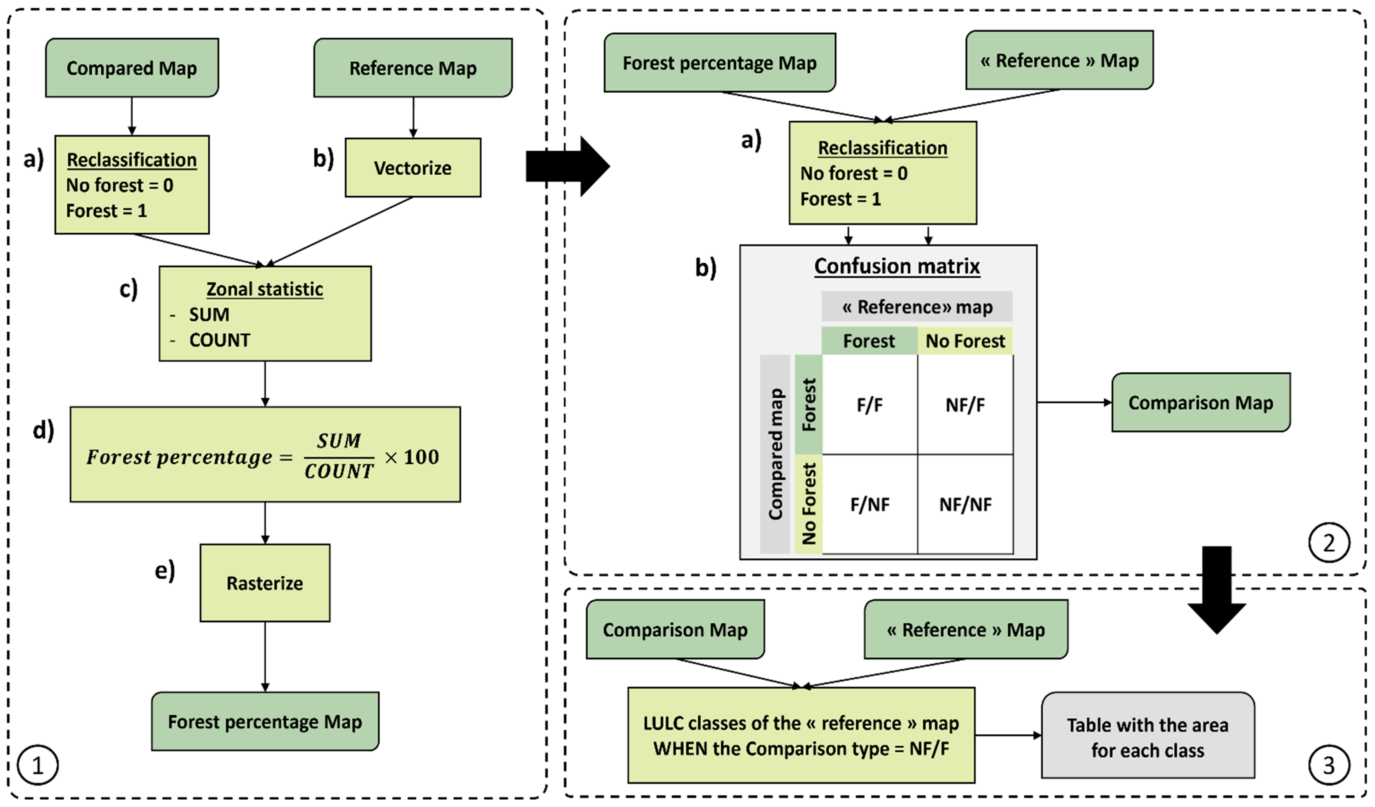
The processing described below was applied to each available common year of the datasets (2005, 2010, and 2015). The map labeled “reference” has the lowest original resolution. The other map labeled “compared” has the highest original resolution. To homogenize the representation of forest/non-forest classes across products, we reclassified each category based on the definition of FAO that defines a forest as an assembly of trees higher than 5 m, with a tree cover higher than 10%. Information on tree cover and height was not present in all the datasets. We tried to match the FAO definition as closely as possible. However, some compromises had to be made (Table A3, Table A4, Table A5, Table A6, Table A7 and Table A8). Thus, all the databases were reclassified according to forest (mask value of 1) and non-forest (mask value of 0) designations based on their original class definition (Figure 2(1a,2a)).
Each reclassified product was then resampled at lower spatial resolutions for comparison (Figure 2(1)). The spatial grids of low-resolution datasets (HILDA+, MODIST1/MODISP2, and ESACCI) were used as the reference for resampling (Figure 2(1b)). For each product, we then calculated the proportion, in percentage, of forest for each grid cell as the ratio of the sum of forest pixels over all pixels present in the grid cell (Figure 2(1c–e)). As GFW includes a continuous tree-cover percentage, mean percentage was calculated to keep the information. Finally, a new forest/non-forest mask was calculated again from the resampled maps following the FAO forest definition (tree cover > 10%; (Figure 2(2a))).

2.4. Spatiotemporal Analyses

We assessed the influence of homogenization and resampling by calculating the mean area of forest and non-forest for each product at each resolution.
We performed an intercomparison of each resampled and newly defined products to assess the agreement and disagreements between them. Products were compared two by two for each common year (2005, 2010, and 2015) to produce a confusion matrix, which is defined as follows: “NF/NF” was attributed if both products observed non-forest; “F/F” if both products observed forest; “F/NF” if the “reference” product observed forest but the “compared” product did not; and NF/F if the “compared” product observed forest but the “reference” product did not (Figure 2(2b)). We then calculated the agreement (Equation (1)) and disagreement (Equation (2)) rate based on this score for each pair of datasets, with agreement + disagreement = 100%.
A g r e e m e n t = M e a n N F / N F + M e a n F / F M e a n N F / N F + M e a n F / F + M e a n F / N F + M e a n N F / F × 100 ( % )
D i s a g r e e m e n t = M e a n F / N F + M e a n N F / F M e a n N F / N F + M e a n F / F + M e a n F / N F + M e a n N F / F × 100 ( % )
where Mean is the area averaged over the target years. Finally, we determined which land-cover (LC) classes were involved in the NF/F differences between the different pairs of databases. We grouped the LC classes of the different datasets into common classes based on the IPCC classification [29]. We defined 8 classes: agriculture, grassland, wetland, settlement, shrubland, sparse vegetation, water, and others. For most of these new classes, the class was already present in the previous definition. The class agriculture also included definitions mentioning “cropland” or “cultivation”. In the case of GLCLU, we defined shrublands as trees lower than 5 m, sparse vegetation as short vegetation with less than 10% of cover, and grassland as short vegetation with cover between 11 and 100% (Table A3, Table A4, Table A5, Table A6, Table A7 and Table A8). We calculated the mean area over the years and the percentage that each class represented.
The temporal evolution of the forest cover from the different LULC products used in this study was analyzed at their original resolution to quantify forest loss and gain. Most datasets cover the period from 2001 to 2019. However, as the GLCLU only provides information on changes over a five-year period, maps from 2005, 2010, and 2015 were used for this analysis. With GFW, we were only able to quantify forest loss, as the map does not provide information on reforestation, except in the form of a cumulative map covering 2001–2012. Where the maps allowed for calculation, we derived net changes in forest area at a yearly timescale. The cumulative sum of these net changes was then calculated to highlight the major trends in the evolution of forest cover for each dataset.
This work was carried out using Python version 3.13.5 and R Studio version 4.3.2.

3. Results

3.1. Impact of Data Homogenization and Resampling on Forest/Non-Forest Masks

3.1.1. Congo Basin

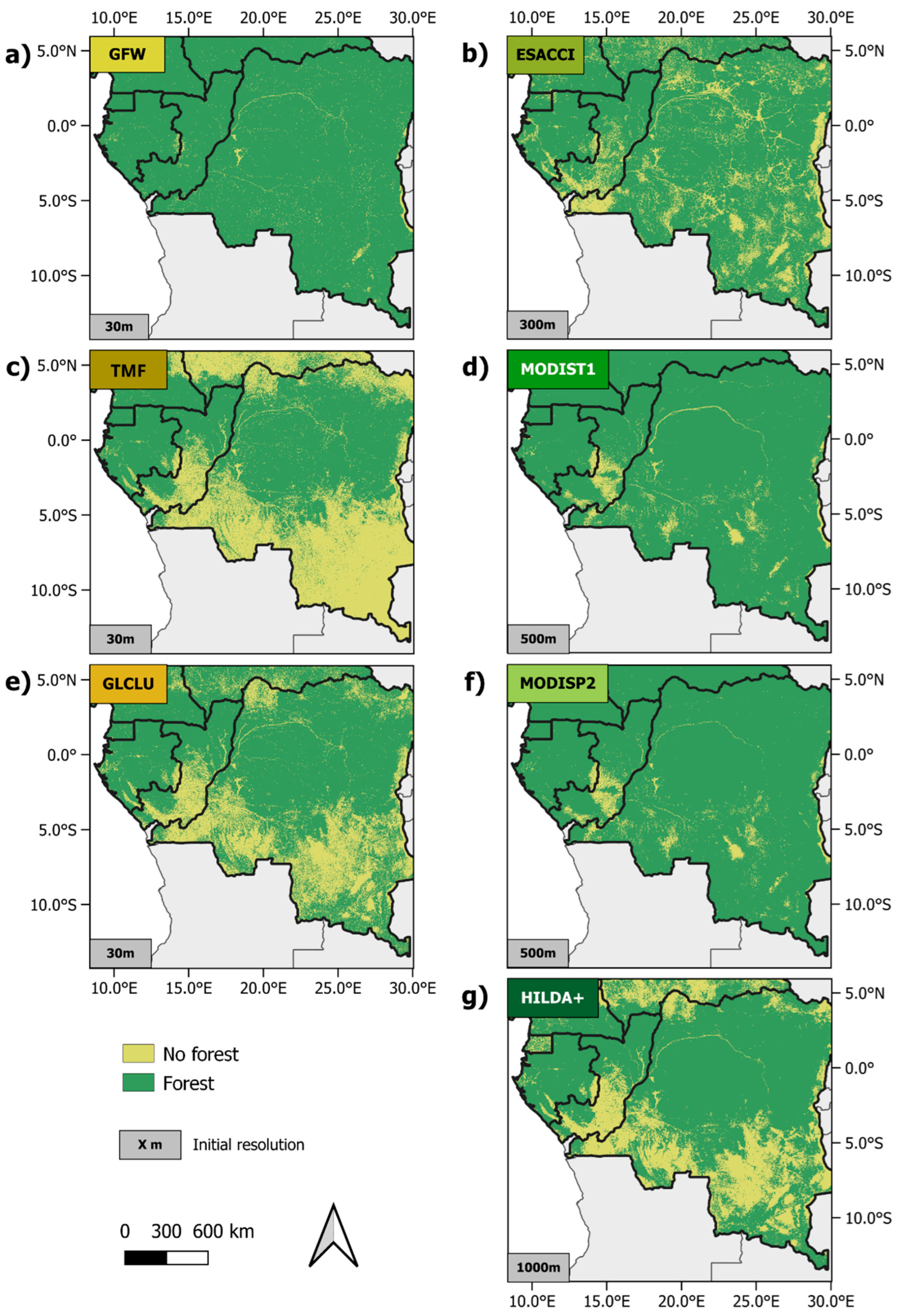
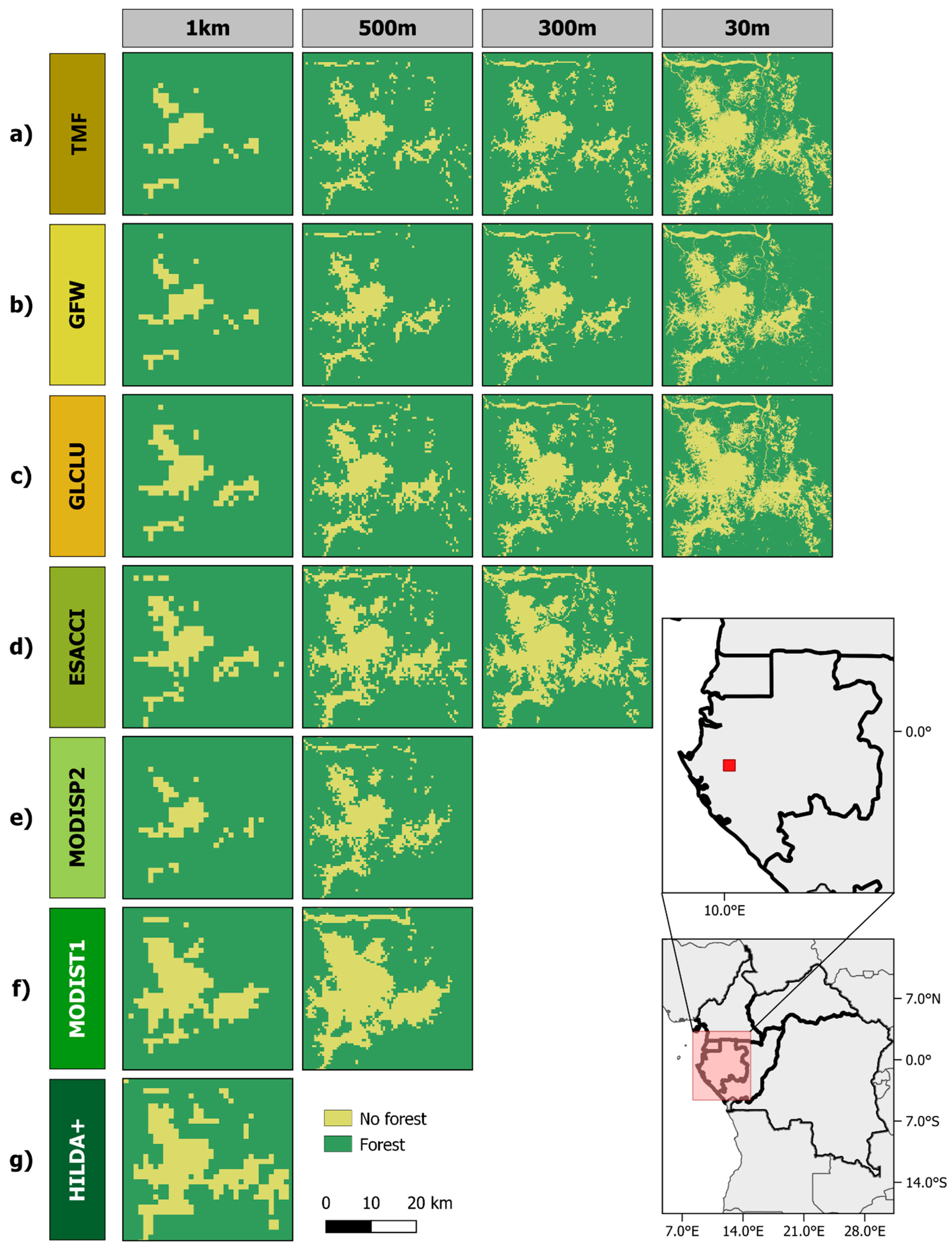
The datasets showed different spatial patterns of forest area (Figure 3). The lower the resolution, the higher the percentage of forest (Figure 4 and Table 2). For example, GLCLU from 30 m to 1 km had forest proportion of 74.10% and 88.51%, respectively (Table 2). Datasets with the highest area of forest at their original resolution were MODIST1, with 94.71%; MODISP2, with 95.23%; and GFW, with 96.37% (Table 2). Datasets with the highest fraction of non-forest at their original resolution were GLCLU, with 25.9%; HILDA+, with 30.16%; and TMF, with 41.4% (Table 2).

3.1.2. Miombo Forest

Over the miombo, GFW, MODIST1, and MODISP2 detected forest cover of 96.1%, 96.4%, and 96.7%, respectively, at their original resolution (Table 2). HILDA+, GLCLU, and ESACCI provided intermediate results in terms of forest cover, with 52.1%, 55.4%, and 77.8%, respectively (Table 2). The major change with decreasing resolution was observed for GLCLU, with a forest gain of 24.1% between 30 m and 1 km (Table 2).

3.1.3. Moist Forest

All the datasets showed a very high forest cover, varying between 88.7% and 98.7%, at their original resolution (Table 2). ESACCI was the dataset with the lowest forest cover (88.7%), and TMF showed the largest increase in forest cover (7.2%) between the original resolution and the 1 km resolution (Table 2).

3.1.4. Savanna Forest

For the savanna ecoregion, the datasets with the highest proportion of forest were MODIST1, MODISP2, and GFW, with values of 90.3%, 90.5%, and 96.5%, respectively (Table 2). The datasets with lower forest cover were TMF, HILDA+, and GLCLU, with values of 30.5%, 44.0%, and 54.6%, respectively (Table 2). The change in resolution affected the proportion of forest, especially for TMF, which showed an increase of 26.8% between 30 m and 1 km resolution.

3.2. Forest/Non-Forest Agreement and Disagreement Between Products

3.2.1. The Congo Basin

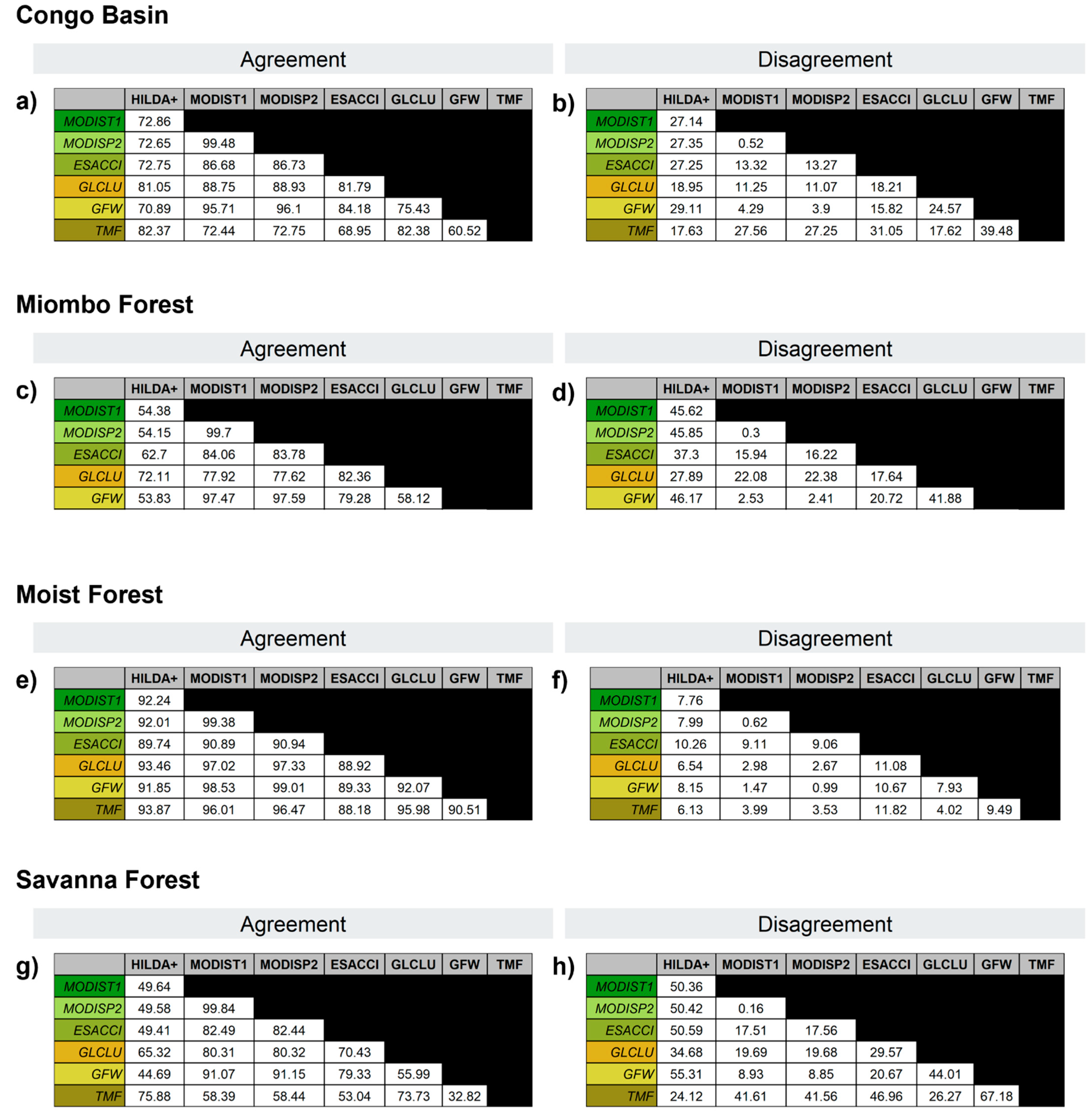
For the Congo Basin, the agreement for all comparisons was between 60.5% and 99.5% (Figure 5a). The higher proportion of disagreement was observed between TMF and GFW, with 39.5% (Figure 5b), while best agreement was obtained between MODIST1 and MODISP2, with 99.48% (Figure 5a).

3.2.2. Miombo Forest

In the case of the miombo, agreement ranged from 53.83% to 99.7% across all comparisons (Figure 5c). Disagreement was high for HILDA+, at 45.62%, 45.85%, and 46.17%, when it was compared to MODIST1, MODISP2, and GFW, respectively (Figure 5d). Meanwhile, the best agreement was obtained between MODIST1 and MODISP2, with 99.7% (Figure 5c).

3.2.3. Moist Forest

For moist forest, there were few discrepancies between the datasets. Agreement was higher than 88.2% for all comparisons (Figure 5e). The higher discrepancy rate was observed between ESACCI and GLCLU or TMF, with 11.0% and 11.8%. (Figure 5f), while the best agreement was obtained between MODIST1 and MODISP2, with 99.38% (Figure 5e).

3.2.4. Savanna Forest

Agreement across the savanna ranged from 32.8% to 99.8% (Figure 5g). Higher discrepancies were observed at 1 km resolution for the majority of the datasets, ranging from 34.7% to 55.3% (Figure 5h). Only TMF showed a higher disagreement rate (67.2%) at 30 m resolution when it was compared to GFW (Figure 5h). Meanwhile, the best agreement was obtained between MODIST1 and MODISP2, with 99.84% (Figure 5g).

3.3. Identification of Land Classes Implicated in the Disagreements

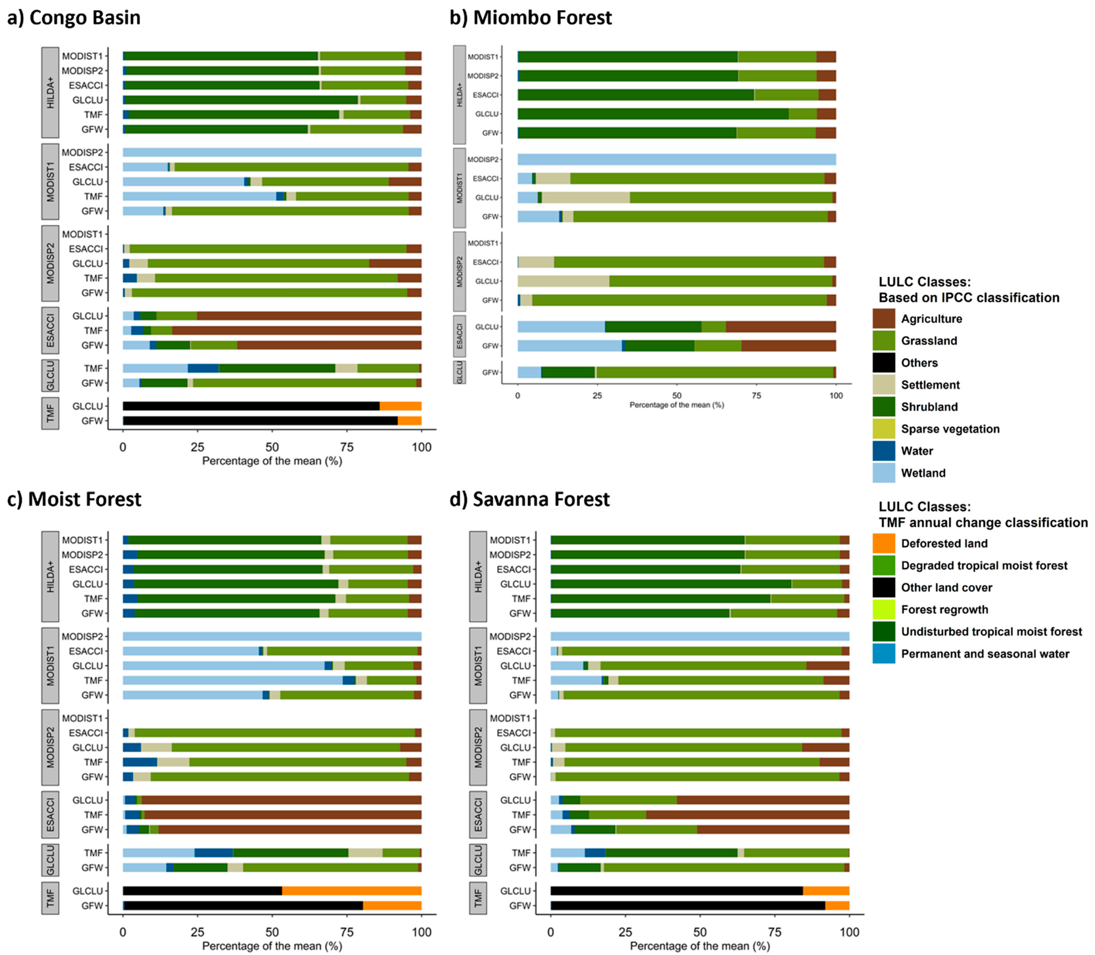
The analysis of the LULC classes implicated in the NF/F differences showed different results depending on the ecoregions and the datasets.

3.3.1. Congo Basin

In the case of the Congo Basin, in terms of NF/F disagreement, HILDA+ detected mainly “shrubland” (up to 77.8%) when the second datasets detected forest (Figure 6a). MODIST1 detected mainly “grassland” (up to 79.3%) and “wetland” (up to 100%; Figure 6a). For MODISP2, the differences were mostly “grassland” (up to 92.7% for ESACCI; Figure 6a). The ESACCI dataset observed mostly “agriculture” (between 61.8% and 83.5%) instead of forest in the other datasets (Figure 6a). When TMF observed forest, GLCLU detected mostly “shrubland” (39.0%); for GFW, GLCLU detected mostly “grassland” (74.7%; Figure 6a). For TMF, the NF/F differences were related to the “deforested” class (up to 14%) and the “other land cover” class (up to 91.8%; Figure 6a).

3.3.2. Miombo Forest

In the case of miombo, HILDA+ detected mostly “shrubland” (up to 85.1%) where the second datasets observed forest (Figure 6b). Two LULC classes were involved in the NF/F differences for MODIST1 (Figure 6b): “wetland”, which accounted for between 4.5% and 100% of the differences (Figure 6b), and “grassland”, which accounted for up to 79.9% of the differences (Figure 6b). MODISP2 showed disagreement mostly for “grassland”, from 70.0% to 92.6%, when the other datasets showed disagreement for forest (Figure 6b). For ESACCI, when compared to GLCLU or GFW, most of the NF/F differences were due to the “shrubland” class (up to 30.1%), “wetland” class (up to 32.7%), or “agriculture” class (up to 34.6%; Figure 6b). When comparing GLCLU and GFW, GLCLU detected a majority of “grassland” (74.3%) when GFW observed forest (Figure 6b).

3.3.3. Moist Forest

For moist forest, HILDA+ detected mostly “shrubland” (up to 68.4%). “Wetland” was implicated in the NF/F differences when MODIST1 was the first dataset (Figure 6c), with up to 100%. MODISP2 showed disagreement mostly for “grassland”, from 76.5% to 93.8%, when the other datasets showed disagreement for forest (Figure 6c). ESACCI detected “agriculture” (>88.1%) most of the time when the other datasets detected forest (Figure 6c). In the case of TMF, the classes involved in the NF/F differences are “deforested land” (19.6%–46.7%) and “other land cover” (53.2%–79.8%; Figure 6c).

3.3.4. Savanna Forest

Across the savanna ecoregion, HILDA+ observed mostly “shrubland” (59.6%–80.5%), while the other datasets observed forest (Figure 6d). MODIST1 and MODISP2 showed similar results, with a majority of “grassland” (up to 95.9%; Figure 6d). ESACCI detected mainly “agriculture” (51%–68.0%; Figure 6d). For GLCLU, the result was split between “shrubland” (14.1%–44.2%) and “grassland” (35.1%–80.5%; Figure 6d). TMF showed a small part of “deforested land” (8.1%–15.6%) and mainly “other land cover” (84.4%–91.8%; Figure 6d).

3.4. Temporal Evolution of the Forest for Each Dataset

3.4.1. The Congo Basin

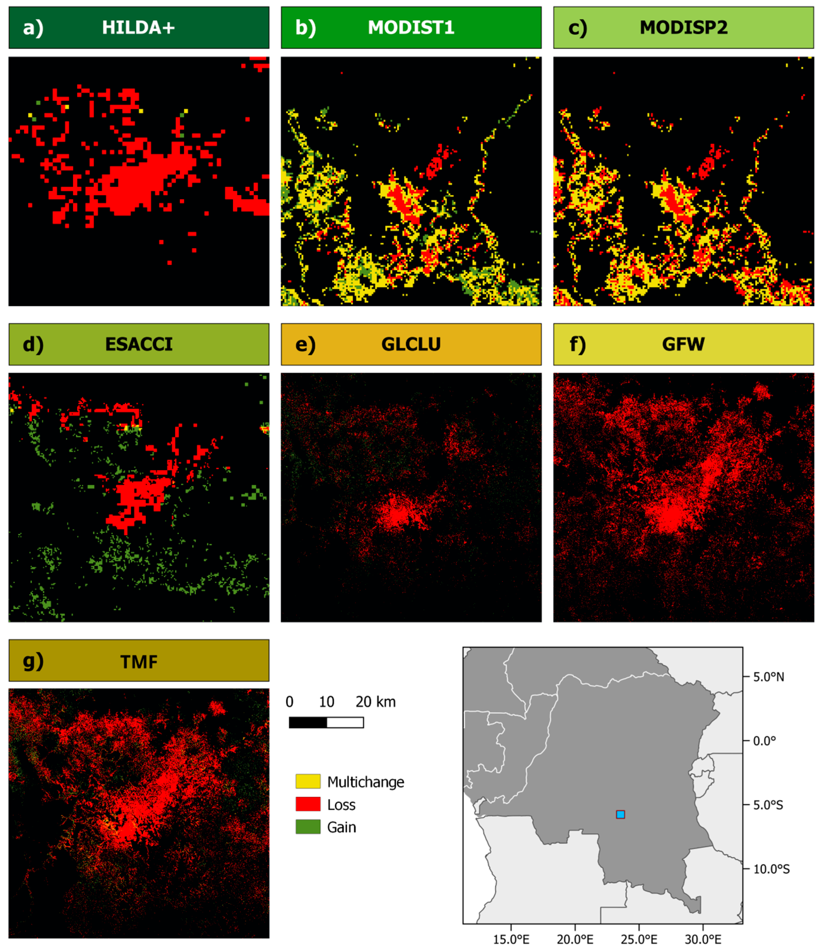
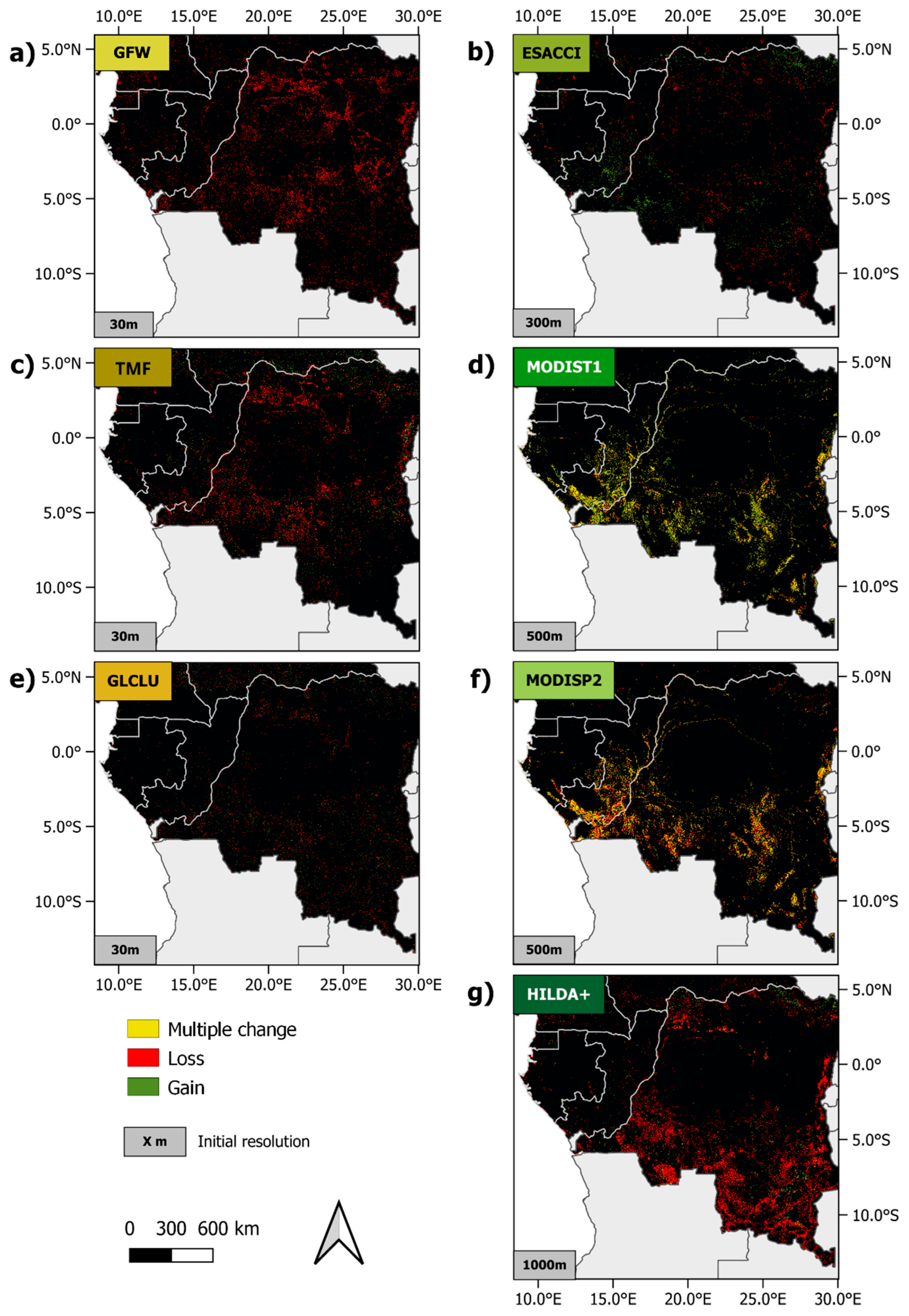
Figure 7 shows the deforestation and reforestation maps for each dataset from 2001 to 2019. GFW, TMF, GLCLU, and HILDA+ all exhibited similar patterns, highlighting large areas of deforestation in the DRC (Figure 7a, Figure 7c, Figure 7e, and Figure 7g, respectively). However, the intensity and spatial patterns of deforestation varied between datasets. Higher deforestation intensity was observed for HILDA+, with hotspots in the south, northwest, and east of the DRC (Figure 7g); and for GFW, higher deforestation intensity was observed in the north and center of the DRC, north of the Congo, Gabon, and south of Cameroon (Figure 7a). Lower intensity was observed for TMF in the northwest and southwest (Figure 7c), and the lowest intensity was observed for GLCLU, with a similar pattern to TMF (Figure 7e). ESACCI exhibited areas of deforestation of a similar intensity to GLCLU across most of the DRC, except in the southeast, northeast, and southwest, where an increase in forest area was observed. Loss/gain in forest area was also observed in the north and south of Congo (Figure 7b).
Similar patterns of forest-cover change were obtained using MODIST1 and MODISP2 (see Figure 7d and Figure 7f, respectively), with large areas of reforestation and multiple changes observed in the southern part of the area and along the Congo River and its tributaries. Figure A6 illustrates these differences in the DRC. In the south of the DRC, similar patterns of deforestation at different spatial resolutions are obtained using HILDA+, GFW, TMF, and GLCLU, while ESACCI presents a pattern of both deforestation and reforestation. The two MODIS-based products exhibit a completely different spatial distribution of changes, and this distribution seems to be partly related to flood dynamics.
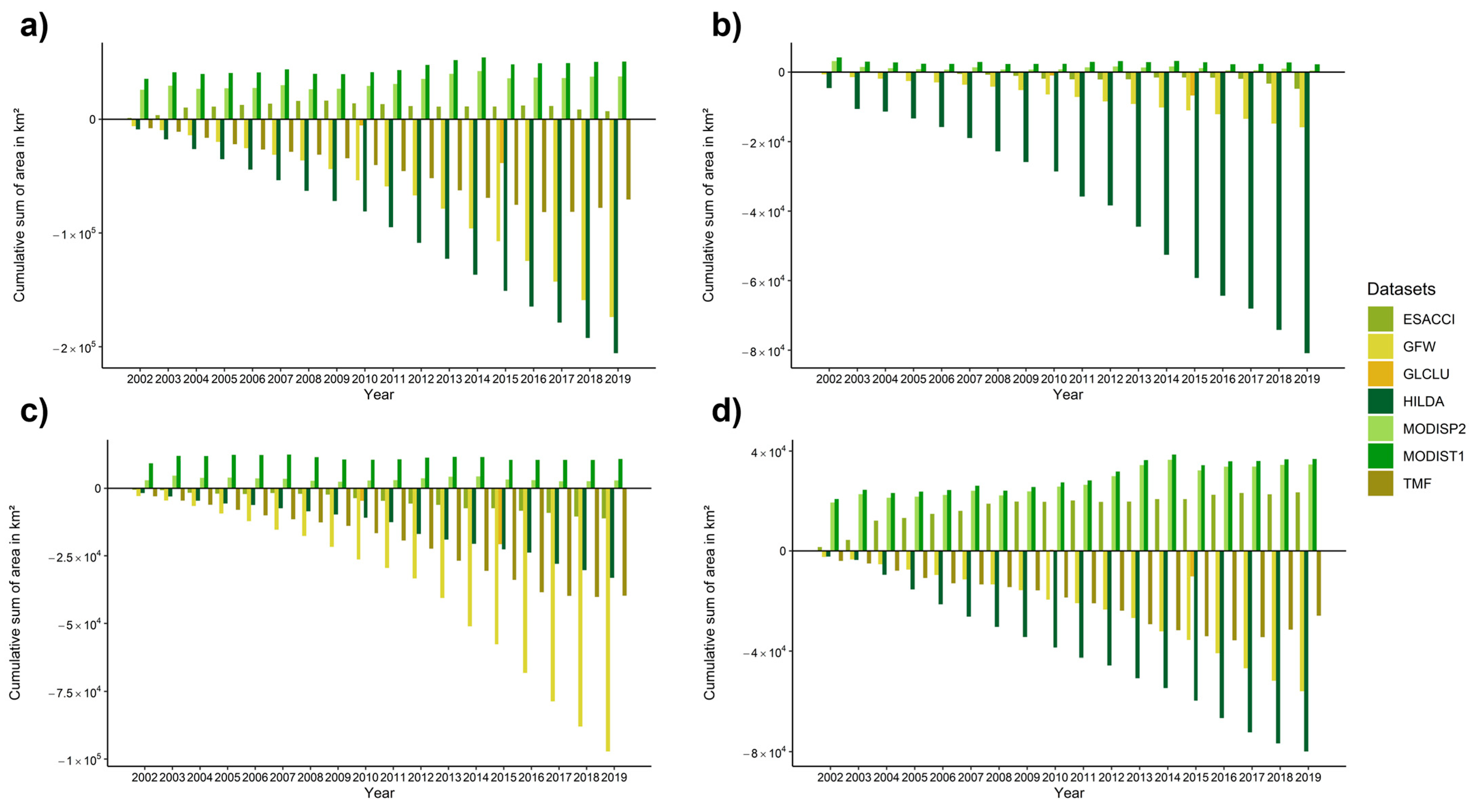
When the temporal evolution was considered, two different behaviors emerged among the datasets. The first behavior corresponded to datasets that exhibited a net forest gain by the end of the study period (i.e., around 2019). The second behavior corresponded to datasets showing a net forest loss by the end of the period. The ESACCI, MODISP2, and MODIST1 products detected a net forest gain ranging from 7063 km2 (ESACCI) to 50,726 km2 (MODIST1) by the end of the period (Figure 8a). In contrast, the HILDA+, GFW, TMF, and GLCLU products detected a net forest loss ranging from 70,601 km2 (TMF) to 205,704 km2 (HILDA+; Figure 8a).

3.4.2. Miombo Forest

Over the miombo region, the MODISP2 and MODIST1 datasets observed net forest gains of 439 km2 and 2248 km2, respectively (Figure 8b). All of the other datasets observed net forest loss (Figure 8b). Notably, HILDA+ revealed a total net forest loss of 80,884 km2 between 2001 and 2019 (Figure 8b), with significant variability in the intensity of this loss across the years.

3.4.3. Moist Forest

Over moist forests, MODISP2 and MODIST1 recorded net forest gains, peaking in 2003 at 4684 km2 and in 2007 at 12,505 km2, respectively (Figure 8c). The other datasets observed net forest loss over the period (Figure 8c). Notably, GFW showed a total net loss of 97,218 km2 (Figure 8c) by the end of the timeline, with an acceleration of deforestation between 2013 and 2019.

3.4.4. Savanna Forest

Three datasets recorded a net forest gain over the considered period in savanna forests: ESACCI (up to 23,451 km2), MODISP2 (up to 36,479 km2 between 2001 and 2014), and MODIST1 (up to 38,580 km2 between 2001 and 2014). The dynamics were different between ESACCI and the MODIS products, with the latter showing net gain in forest cover for some years. TMF, HILDA+, and GFW showed net forest loss over the same period (Figure 8d). The same dynamic was observed for HILDA+ and GFW datasets, which showed net forest loss throughout the period. In contrast, TMF observed net forest gain between 2017 and 2019 (Figure 8d).

4. Discussion

The comparison of forest/non-forest masks required a common definition of forest. In this study, we matched the FAO definition, which considers a pixel to be covered with forest when (i) having a tree cover of more than 10% and (ii) a tree height of more than 5 m [30]. This definition has the advantage of being based on two criteria that are regularly present in the definition of LULC classes in the databases that were used in this study. The two criteria were respected as much as possible, but the first reclassification could not meet all the requirements (Table A3, Table A4, Table A5, Table A6, Table A7 and Table A8). This leads to differences in the forest area between the datasets. Considering all the resolutions over all the studied regions, GFW, MODIST1, and MODISP2 presented a larger forest area than the other dataset. In the case of GFW, this could be explained by an overestimation of tree cover. A lack of distinction between tropical forest, plantations, and herbaceous cultivation in this product was reported over tropical regions [31]. Furthermore, the tree-cover map is only available for the year 2000. It is possible that other changes (degradation by selective logging or climate events) which occurred between 2000 and 2015 were not included in the analysis. This difference could also be explained by the 10% threshold used to define forests. A previous study showed that the value of 70% tree cover was closer to reality than a value of 30% for Gabon [32]. The choice of the tree-cover threshold for forest definition, in the case of the GFW map, is crucial and must be taken into account in the analysis. The larger forest area of MODIST1 and MODISP2 could be explained by the low resolution of 500 m. Since forest disturbances in this region are smaller than in other parts of the world, areas where there is non-forest could be missed due to the low resolution. Furthermore, in their definition of forest, the MODIS products include trees higher than 2 m. This leads us to consider a larger proportion of the savanna as forest, given that the trees are shorter than those in the moist forest or miombo woodlands. Observations made in tropical Asian forests reported that MODIS land-cover products are not able to distinguish plantations from natural forests [33], and this fact could account for the probable overestimation of forest area also in Africa. The datasets which presented the smaller forest area for the studied Congo Basin region were HILDA+, ESACCI, GLCLU, and TMF. Concerning HILDA+, an explanation could be found in the tree-cover threshold of 25%, which is associated with its low resolution and the lack of statistical information on Africa. Regarding ESACCI, the result could be due to the dataset’s difficulty in assigning the mosaic classes to the forest/non-forest masks and the use of satellites with different resolutions [34]. GLCLU also presented a smaller forest area in the majority of the ecoregions. Probably due to the definition of a forest mask only based on tree height, savanna with a low tree height was classified as non-forest. Even if GEDI offered more precision regarding the tree height, it still had limitations. Notably, in case of high slope and dense forest canopy [35,36], which can explain part of the results. The TMF showed a low forest area over all of the Congo Basin (58.6% at 30 m resolution) and savanna (30.46% at 30 m resolution). This is most likely due to the fact that TMF provides information on tropical moist forests, which represent a smaller proportion of forest cover in the savanna and miombo regions (generally over 50% in the other products in these two regions).
Most of the differences in forest area could be explained by the definition of forest. These differences in definition lead to difficulties in reclassification and are likely to account for most of the differences between the databases. The reclassification of forests in GLCLU is based on tree height (>5 m), while that of GFW is based on tree cover (>10%). At the same resolution, the datasets disagreed by 24.57% over the Congo Basin and by 44.01% over savanna forest. This contrasts with the case of MODIST1 and MODISP2, which exhibited a disagreement of 0.52% at their original resolution over the Congo Basin (Figure 5). Their reclassification is very similar, based on both tree cover (>10%) and tree height (>2 m). The only difference lies in the definition of “permanent wetland” in MODIST1, which includes vegetation cover of more than 10%, without specifying the type of vegetation (Figure 6 and Table A4). These results demonstrate that when the same definition of forest is used, including both tree cover and height, the consistency between the datasets can be high. Our work highlights the urgent need for a common definition of forests in LULC classifications to facilitate the use and the interpretation between products. Two pieces of information need to be included in the definition of the classes made up of trees: tree cover and tree height. Sannier et al. [32] reported the influence of the region on the choice of the tree-cover threshold. A threshold adapted to the forest type could allow for a better definition of the forest/non-forest mask [32]. As shown by the MODIS products and the GLCLU over the savanna, the threshold for tree height also impacts the results (Table 2, Table A4, Table A5 and Table A7). By incorporating tree cover and height into the definition of future maps, users can select an appropriate threshold for their needs and the ecoregion of interest. The choice of resolution also affects the estimated area of forest/non-forest. This area varied due to the resampling, regardless of the datasets. The lower the resolution, the greater the amount of forest, regardless of the ecoregion considered. For example, GLCLU presented forest areas of 54.58% and 91.87% at a resolution of 30 m for savanna and moist forest, respectively. At 1 km, these percentages increased to 78.25% for savanna and 97.87% for moist forest. This result shows that a low resolution can lead to an overestimation of forest cover. Resolution also has an impact on the detection of land-cover change. Deforested areas in Africa are small and difficult to detect using remote-sensing techniques [20]. It is essential to work at a high resolution when it comes to Africa and use satellites with better spatial resolution [37].
The LULC classes mostly implicated in the disagreement between the datasets were “agriculture”, “grassland”, and “shrubland”. This result highlights the difficulties faced by remote sensing when making distinctions between different vegetation types, notably in tropical regions. These results could be explained by the signal saturation of remote-sensing data. In the case of dense vegetation or high biomass, the optical or Synthetic Aperture Radar (SAR) signals may saturate [38,39], leading to a lack of change detection or differentiation between different types of vegetation [38]. The study of vegetation phenology can be helpful for vegetation-type discrimination [40]. The ecoregions with the higher level of disagreement between datasets were miombo and savanna, which presented the higher seasonality, highlighting the importance of monitoring throughout the year. However, given the high cloud cover in the tropics, optical remote sensing cannot offer a sufficient number of cloud-free images to meet the requirements of continuous monitoring [10]. This limitation could be overcome by adding other sensors to create complementarity between data sources. Optical remote sensing provides information on vegetation photosynthesis activity, while Light Detection and Ranging (LiDAR) and Synthetic Aperture Radar (SAR) offer new, relevant insights into forest structure and vegetation water content [41,42,43,44]. Furthermore, SAR sensors are less sensitive to saturation and can penetrate cloud cover, thus increasing the number of images acquired per year. Recent forest cover-monitoring products, which are not included in this study, as they do not cover the same period, are based either on SAR images or on the fusion of SAR and multispectral images [42,45]. They were found to have a higher level of accuracy than products based solely on multispectral information [46] and to identify deforestation sooner, as well as to be able to detect both deforestation and degradation in equatorial areas [42,44]. Forest-height products based on merging multispectral and SAR images with LiDAR-based tree heights are likely to provide unique information on forest cover and regrowth [47,48,49].
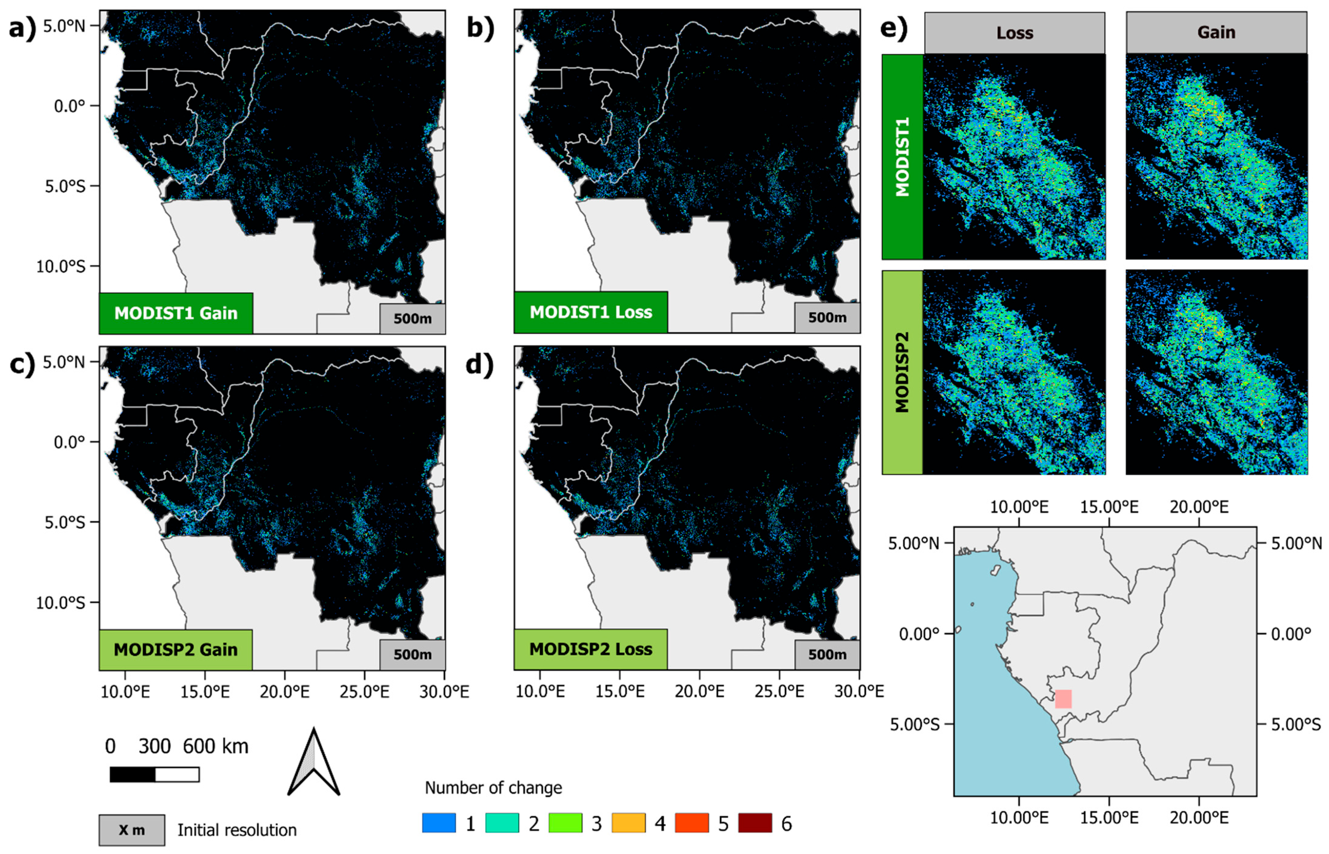
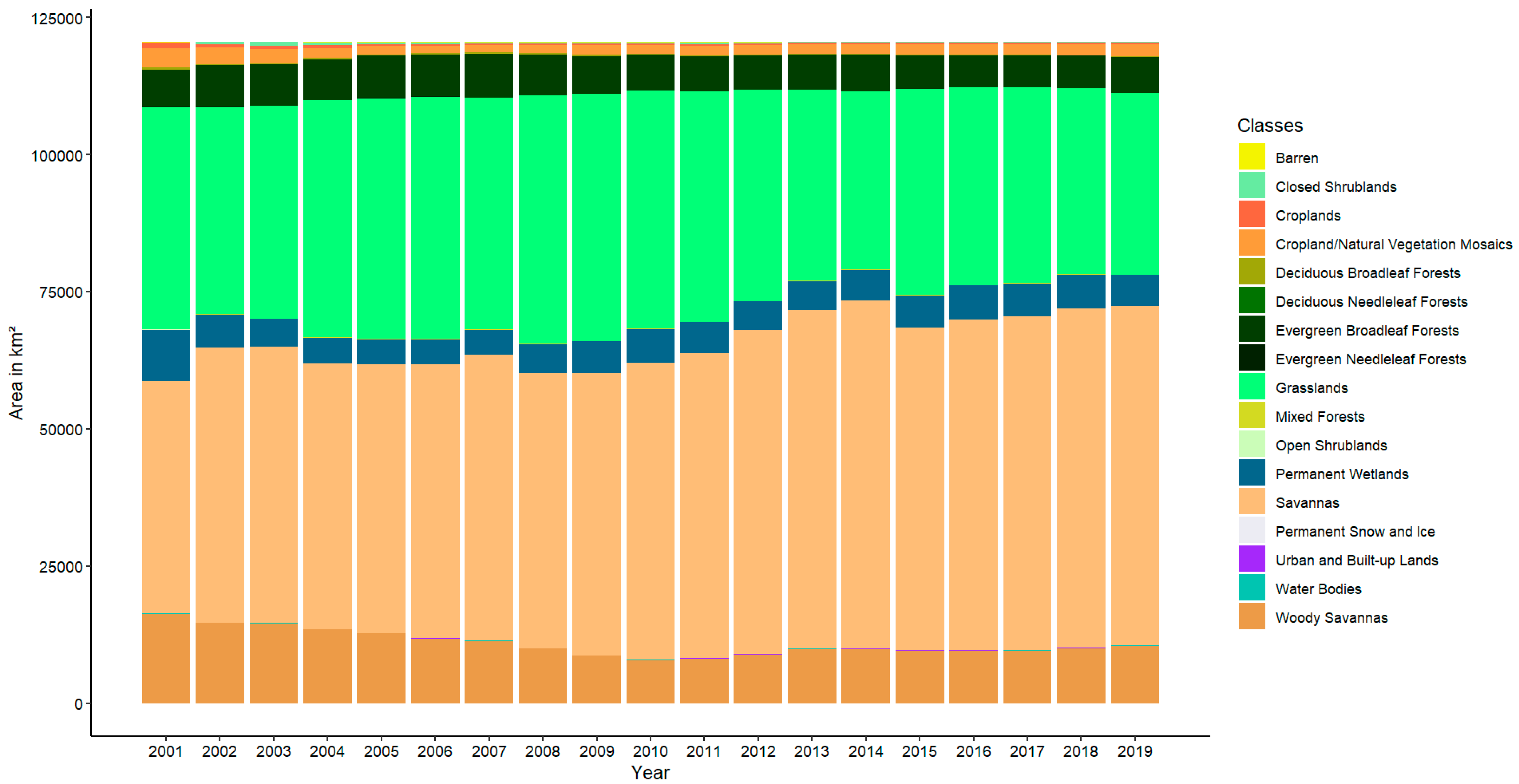
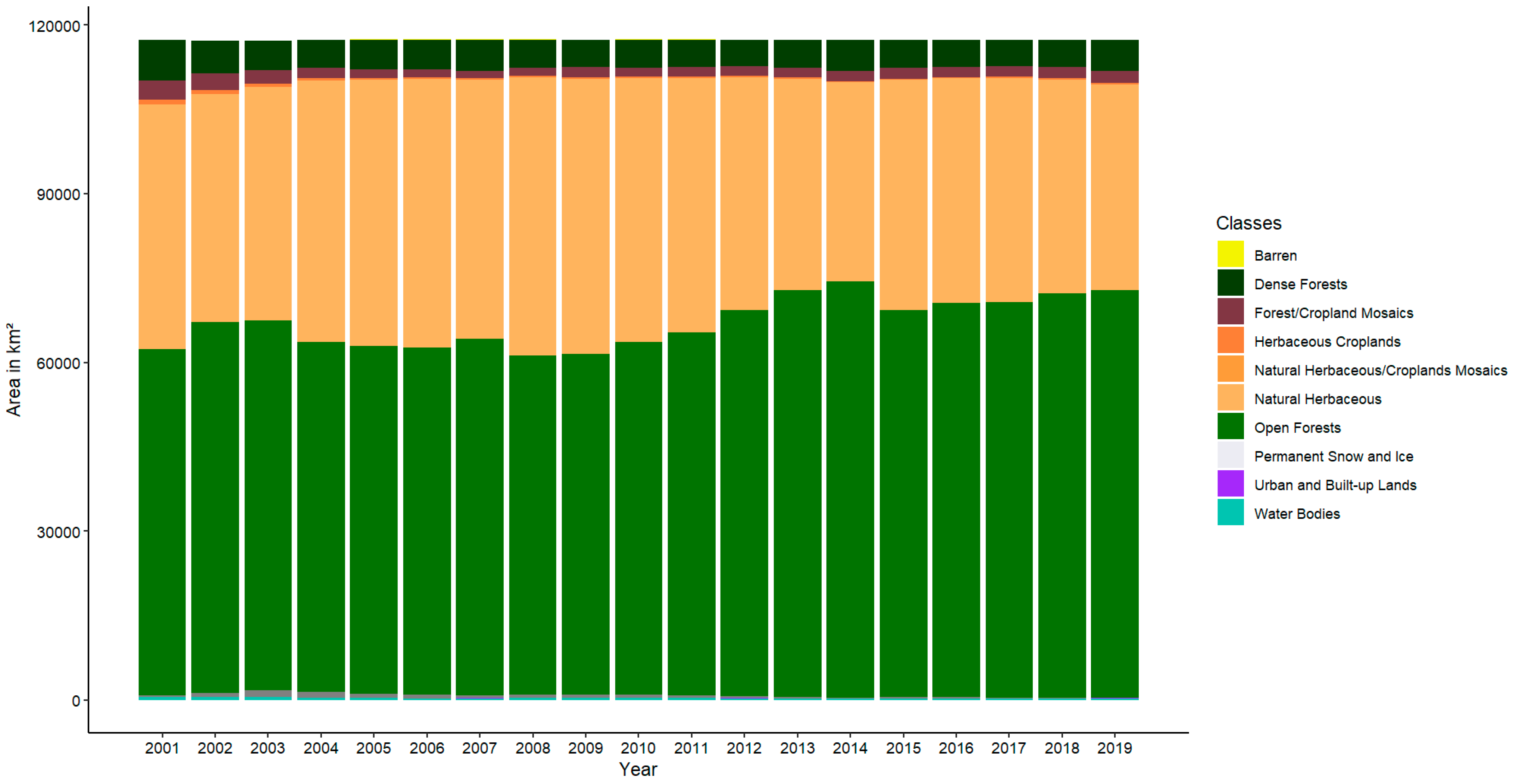
Temporal analysis of the forest cover revealed that datasets with low resolution tend to show a net gain across the study region and period (MODIST1, MODISP2, and ESACCI). This is probably due to the sensors’ resolution not allowing small changes to be detected. The only exception is HILDA+, which has a resolution of 1 km and tends to observe a net loss of forest over the period. This could be explained by the algorithm used to generate the HILDA+ product, which took into account multiple remote-sensing datasets, as well as statistical data from the FAO. Since this dataset is based on statistics, it is less impacted by the above-mentioned image-processing issues and took advantage of multiple sources of information to provide a robust estimation [17]. Furthermore, this dataset has already been shown to demonstrate good accuracy over the tropical forests of Ecuador compared to TMF, even with a resolution of 1 km [50]. The forest gain was most significant in the savanna ecoregion, with a net gain of 36,827 km2 at the end of the period for MODIST1. It is well known that the woody cover of the savanna in this region is highly unstable due to the mean annual precipitation [51]. This ecosystem characteristic, coupled with the low resolution of the sensors and the limited availability of optical data, could also account for the large alternance between forest gain and loss from one year to another observed in the products. GFW observed higher rates of forest loss over the moist ecoregion, with a net loss of 97,217 km2 by the end of the period. The high resolution of Landsat (30 m) enables the detection of small-scale deforestation and degradation, which is typically observed in tropical Africa. Some datasets recorded gains and losses in the same region over the study period. This is notably the case for MODIS products (Figure 7, Figure A6 and Figure A7). Despite the incorporation of the hidden Markov model (HMM) in Collection 6 to stabilize classification over time, some pixels appear to be subject to high dynamics [16]. Areas of 11,746 km2 and 12,045 km2 were detected as having experienced at least one loss-and-gain event for MODISP2 and MODIST1, respectively (Figure A7). Analysis of the classes at these locations showed that they were mostly “savanna” and “grassland” for MODIST1, and “open forest” and “natural herbaceous” for MODISP2 (Figure A8 and Figure A9). These classes have very similar definitions in terms of tree cover or height, and these similarities in definitions could explain why a small difference in the signal could result in a different class attribution (Table A4 and Table A5).

5. Conclusions

In this study, seven of the most-used forest-cover datasets (HILDA+, MODIST1, MODISP2, ESACCI, GLCLU, GFW, and TMF) were compared across different ecoregions of the Congo Basin. Our goal was not only to provide an intercomparison but also to identify in which classes they differ. This required homogenization of the forest definition in order to resample the datasets at the same spatial resolution. In this context, a forest was defined as an area with tree cover of more than 10% and trees of more than 5 m in height. However, information on these two parameters is not always available in the class definition. Through this methodology, we have emphasized the importance of these two criteria and of taking the threshold into account, depending on the ecoregion being studied. The change in resolution influenced the forest area, with a probable overestimation at coarser resolution. For example, the GLCLU forest cover increased from 74.10% to 88.51% at 30 m and 1 km resolution, respectively. This result can be explained by the small areas of deforestation in Africa that are not detected at low resolution. Comparison of the different datasets across ecoregions showed higher levels of inconsistency for miombo (around 24.3%) and savanna (around 32%). Further analysis showed that the majority of LULC classes involved in the differences between datasets across ecoregions were related to “shrubland” (up to 77.8%), “agriculture” (up to 83.5%), and “grassland” (up to 92.7%). This illustrates the difficulty in distinguishing vegetation types using remote-sensing data. These results could be explained by the use of optical sensors, which provide few images per year due to cloud cover. This prevents the monitoring of phenology, which is a key information for vegetation type. The inclusion of new information from SAR images and LiDAR canopy heights could improve the results of future maps and provide a new understanding of African forest dynamics. For now, the presented datasets exhibited different behavior with regard to the evolution of forest cover. While other datasets observed a net loss of up to 205,704 km2, MODIS products and ESACCI exhibited a net gain of up to 50,726 km2 during the period of 2001–2019. This trend was apparent across all ecoregions, reflecting inconsistencies between the datasets. This work demonstrated that different conclusions about the evolution of forest cover can be drawn depending on the product used. Even without ground-truth data, the results concerning forest cover dynamics and the evaluation of inconsistencies between these products can provide valuable insights for conservation planning. This study quantifies the uncertainty and confidence that can be attributed to each product depending on the ecoregion, helping to select the most suitable land-use and land-cover (LULC) maps.

Author Contributions

Conceptualization. F.F. and M.P.; methodology. S.R., F.F., M.P., and V.S.; supervision. F.F. and M.P.; visualization. S.R.; writing—original draft. S.R.; writing—review and editing. F.F., M.P., V.S., J.-P.W., P.C., and B.Y. All authors have read and agreed to the published version of the manuscript.

Funding

Solène Renaudineau was supported by a PhD grant from the French National Institute for Agriculture, Food and Environment (INRAE) through ECODIV Scientific Division. This work has been supported by the Programme National de Télédétection Spatiale (PNTS, grant N°PNTS-2023-11—TestReTroForRS). We are grateful to the One Forest Vision initiative, funded by the Ministry of Higher Education and Scientific Research and the Ministry of Europe and Foreign Affairs, for their support. Valentine Sollier is supported by a PhD from MELICERTES (ANR-22-PEAE-0010) project of the French National Research Agency under the France2030 program in the framework of the national PEPR “agroécologie et numérique”.

Data Availability Statement

The original contributions presented in this study are included in the article. Further inquiries can be directed to the corresponding author.

Acknowledgments

We would like to thank all the developers and contributors of the LULC datasets, Python version 3.13.5, and R packages version 4.3.2, which are free and open source.

Conflicts of Interest

The authors declare no conflict of interest.

Appendix A

Table A1. Data availability.
Web Address Dataset DownloadDate of DownloadReference Publication
HILDA+https://doi.pangaea.de/10.1594/PANGAEA.921846?format=html#download6 December 2023Winkler et al., 2021 [17]
MODIST1https://appeears.earthdatacloud.nasa.gov/21 March 2024Sulla-Menashe et al., 2019 [16]
MODISP2https://appeears.earthdatacloud.nasa.gov/21 March 2024Sulla-Menashe et al., 2019 [16]
ESACCIhttps://cds.climate.copernicus.eu/datasets/satellite-land-cover?tab=overview4 December 2023ESA. “Land Cover CCI Product User Guide Version 2”. 2017 [15]
GLCLUhttps://storage.googleapis.com/earthenginepartners-hansen/GLCLU2000-2020/v2/download.html1 December 2023Potapov et al., 2022 [14]
GFWhttps://storage.googleapis.com/earthenginepartners-hansen/GFC-2022-v1.10/download.html6 December 2023Hansen et al., 2013 [18]
TMFhttps://forobs.jrc.ec.europa.eu/TMF/data1 March 2024Vancutsem et al., 2021 [19]
Table A2. Definition of the ecoregions based on the Terrestrial Ecoregions of the World.
Miombo Moist ForestSavanna
Angolan miombo woodlandsNorthwestern Congolian lowland forestsNorthern Congolian forest–savanna mosaic
Central Zambezian miombo woodlandsNortheastern Congolian lowland forestsWestern Congolian forest–savanna mosaic
Central Congolian lowland forestsSouthern Congolian forest–savanna mosaic
Atlantic Equatorial coastal forest
Cross Sanaga–Bioko coastal forests
Western Congolian swamp forests
Eastern Congolian swamp forests
Table A3. HILDA+ reclassification, based on Winkler et al., 2021 [17].
General ClassDescriptionForest Mask ClassificationIPCC Class
UrbanArtificial surfaces, and urban and built-up areas, including urban parks and sports areas, green spaces, industrial areas, deposits, and extraction sites (mining, etc.). Non-forestSettlement
Cropland Herbaceous and woody crops (also for hay production), including tree/shrub crops, orchards, plantations, and multiple/layered crops, incl. mosaics (with cropland area fraction > 40%).Non-forestAgriculture
Pasture/rangelandManaged herbaceous plants (cover > 10%), including managed grasslands (e.g., prairies, steppes, savannas, and mosaics with tree/shrubs): grasslands or meadows used for livestock grazing, hay production with different intensities, etc. Non-forestGrassland
ForestTrees with > 5 m height (cover > 10%), including forest plantation, and trees on seasonally or permanently flooded areas, including mangroves.ForestForest
Unmanaged grass/shrublandNatural herbaceous plants (cover > 10%), including grasslands (e.g., prairies, steppes, savanna, and mosaics with tree/shrubs), or natural shrub cover (>10%), including permanently or regularly flooded areas (wetlands) and (herbaceous) wetlands. Non-forestShrubland
Sparse/no vegetation Bare areas, sparse vegetation (2%–10%), snow and ice, rocks, sand, and mudflats.Non-forestSparse vegetation
Water Non-forestWater
Table A4. MODIST1 reclassification, based on Sulla-Menashe et al., 2019 [16].
General Class Description Forest Mask Classification IPCC Class
Evergreen needleleaf forestsDominated by evergreen conifer trees (canopy > 2 m). Tree cover > 60%.ForestForest
Evergreen broadleaf forestsDominated by evergreen broadleaf and palmate trees (canopy > 2 m). Tree cover > 60%.ForestForest
Deciduous needleleaf forestsDominated by deciduous needleleaf (larch) trees (canopy > 2 m). Tree cover > 60%.ForestForest
Deciduous broadleaf forestsDominated by deciduous broadleaf trees (canopy > 2 m). Tree cover > 60%.ForestForest
Mixed forestsDominated by neither deciduous nor evergreen (40–60% of each) tree type (canopy > 2 m). Tree cover > 60%.ForestForest
Closed shrublandsDominated by woody perennials (1–2 m height), >60% cover.Non-forestShrubland
Open shrublandsDominated by woody perennials (1–2 m height), 10%–60% cover.Non-forestShrubland
Woody savannasTree cover of 30%–60% (canopy > 2 m).ForestForest
SavannasTree cover of 10%–30% (canopy > 2 m).ForestForest
GrasslandsDominated by herbaceous annuals (<2 m).Non-forestGrassland
Permanent wetlandsPermanently inundated lands with 30%–60% water cover and >10% vegetated cover.Non-forestWetland
CroplandsAt least 60% of area is cultivated cropland.Non-forestAgriculture
Urban and built-up landsAt least 30% impervious surface area, including building materials, asphalt, and vehicles.Non-forestSettlement
Cropland/natural vegetation MosaicsMosaics of small-scale cultivation of 40%–60%, with natural tree, shrub, or herbaceous vegetation.Non-forestAgriculture
Permanent snow and iceAt least 60% of area is covered by snow and ice for at least 10 months of the year.Non-forestOthers
BarrenAt least 60% of area is non-vegetated barren (sand, rock, and soil) areas with less than 10% vegetation.Non-forestOthers
Water bodiesAt least 60% of area is covered by permanent water bodies.Non-forestWater
Table A5. MODISP2 reclassification, based on Sulla-Menashe et al., 2019 [16].
General Class Description Forest Mask Classification IPCC Class
BarrenAt least 60% of area is non-vegetated barren (sand, rock, and soil) or permanent snow/ice, with less than 10% vegetation.Non-forestOthers
Permanent snow and iceAt least 60% of area is covered by snow and ice for at least 10 months of the year.Non-forestOthers
Water bodiesAt least 60% of area is covered by permanent water bodies.Non-forestWater
Urban and built-up landsAt least 30% of area is made up of impervious surfaces, including building materials, asphalt, and vehicles.Non-forestSettlement
Dense forestsTree cover > 60% (canopy > 2 m).ForestForest
Open forestsTree cover of 10–60% (canopy > 2 m).ForestForest
Forest/cropland mosaicsMosaics of small-scale cultivation 40%–60%, with >10% natural tree cover.Non-forestAgriculture
Natural herbaceousDominated by herbaceous annuals (<2 m). At least 10% cover.Non-forestGrassland
Natural herbaceous/cropland mosaicsMosaics of small-scale cultivation 40%–60%, with natural shrub or herbaceous vegetation.Non-forestAgriculture
Herbaceous croplandsDominated by herbaceous annuals (<2 m). At least 60% cover. Cultivated fraction >60%.Non-forestAgriculture
ShrublandsShrub cover >60% (1–2 m).Non-forestShrubland
Table A6. ESACCI reclassification, based on ESA 2017 [15].
Description Forest Mask Classification IPCC Class
Cropland rainfedNon-forestAgriculture
Cropland rainfed—herbaceous coverNon-forestAgriculture
Cropland rainfed—tree or shrub coverNon-forestAgriculture
Cropland irrigated or post-floodingNon-forestAgriculture
Mosaic cropland (>50%)/natural vegetation (tree/shrub/herbaceous cover) (<50%)Non-forestAgriculture
Mosaic natural vegetation (tree/shrub/herbaceous cover) (>50%)/cropland (<50%) Non-forestAgriculture
Tree cover—broadleaved evergreen, closed to open (>15%)ForestForest
Tree cover—broadleaved deciduous, closed to open (>15%)ForestForest
Tree cover—broadleaved deciduous, closed (>40%)ForestForest
Tree cover—broadleaved deciduous, open (15%–40%)ForestForest
Tree cover—needleleaved evergreen, closed to open (>15%)ForestForest
Tree cover—needleleaved evergreen, closed (>40%)ForestForest
Tree cover—needleleaved evergreen, open (15%–40%)ForestForest
Tree cover—needleleaved deciduous, closed to open (>15%)ForestForest
Tree cover—needleleaved deciduous, closed (>40%)ForestForest
Tree cover—needleleaved deciduous, open (15%–40%)ForestForest
Tree cover—mixed leaf type (broadleaved and needleleaved)ForestForest
Mosaic tree and shrub (>50%)/herbaceous cover (<50%)ForestForest
Mosaic herbaceous cover (>50%)/tree and shrub (<50%)Non-forestGrassland
ShrublandNon-forestShrubland
Shrubland evergreenNon-forestShrubland
Shrubland deciduousNon-forestShrubland
GrasslandNon-forestGrassland
Lichens and mossesNon-forestSparse vegetation
Sparse vegetation (tree/shrub/herbaceous cover) (<15%)Non-forestSparse vegetation
Sparse tree (<15%)Non-forestSparse vegetation
Sparse shrub (<15%)Non-forestSparse vegetation
Sparse herbaceous cover (<15%)Non-forestSparse vegetation
Tree cover, flooded fresh or brackish waterForestForest
Tree cover, flooded saline waterForestForest
Shrub or herbaceous cover, flooded fresh/saline/brackish waterNon-forestWetland
Urban areasNon-forestSettlement
Bare areasNon-forestOthers
Consolidated bare areasNon-forestOthers
Unconsolidated bare areasNon-forestOthers
Water bodiesNon-forestWater
Permanent snow and iceNon-forestOthers
Table A7. GLCLU reclassification, Potapov et al., 2022 [14].
General Class Description Forest Mask Classification IPCC Class
Terra firma—true desert3%–7% short vegetation coverNon-forestSparse vegetation
Terra firma—semi-arid11%–75% short vegetation coverNon-forestGrassland
Terra firma—short, dense vegetation79%–100% short vegetation coverNon-forestGrassland
Terra firma—tree cover3–5 m treesNon-forestShrubland
Terra firma—tree cover 6–>25 m trees ForestForest
Wetland—salt pan3%–7% short vegetation coverNon-forestWetland
Wetland—sparse vegetation 11%–75% short vegetation coverNon-forestWetland
Wetland—short, dense vegetation 79%–100% short vegetation coverNon-forestWetland
Wetland—tree cover 3–5 m treesNon-forestWetland
Wetland—tree cover 6–>25 m trees ForestForest
Open surface water 20%–100% of yearNon-forestWater
Snow/iceSnow/iceNon-forestOthers
CroplandCroplandNon-forestAgriculture
Built-up Built-upNon-forestSettlement
OceanOceanNon-forestWater
Table A8. TMF reclassification, Vancutsem et al., 2021 [19].
General Class Description Forest Mask Classification
Undisturbed tropical moist forestClosed evergreen or semi-evergreen forest without any disturbance.Forest
Degraded tropical moist forestClosed evergreen or semi-evergreen forest (covered by existing or regrowing trees) that has been temporarily disturbed during a period of maximum 2.5 years. Forest
Deforested landPermanent conversion of forest into non-forested land that started, at the latest, in the current year. Disturbances were observed over more than 2.5 years, and no vegetative regrowth was detected.Non-forest
Tropical moist forest regrowthPixel that has been deforested before the current year and that is currently regrowing. A minimum 3-year duration (2020–2022) of permanent moist forest-cover presence is needed to classify a pixel as forest regrowth (to avoid confusion with agriculture).Forest
Permanent and seasonal waterThis class includes permanent and seasonal water from the GWS dataset.Non-forest
Other land coverNo data and non-TMF cover, which includes savanna, deciduous forest, agriculture, evergreen shrubland, non-vegetated cover, and afforestation.Non-forest
Table A9. Forest and non-forest areas for all the datasets at each resolution and for all of the studied regions.
Congo BasinMiomboMoist ForestSavanna
DatasetNon-Forest Area
in 106 km2
Forest
Area
in 106 km2
Non-Forest Area
in 106 km2
Forest
Area
in 106 km2
Non-Forest Area
in 106 km2
Forest
Area
in 106 km2
Non-Forest Area
in 106 km2
Forest
Area
in 106 km2
Resolution
HILDA+1.052.430.210.230.161.670.630.491 km
MODIST10.113.370.010.430.021.810.061.061 km
MODISP20.103.380.010.430.011.820.061.061 km
ESACCI0.293.190.050.390.101.730.111.011 km
GLCLU0.403.080.090.350.041.790.240.881 km
GFW0.033.450.010.430.011.820.011.111 km
TMF0.972.51 0.051.780.480.641 km
MODIST10.183.300.020.420.041.790.111.01500 m
MODISP20.173.310.010.420.021.800.111.01500 m
ESACCI0.482.990.080.360.171.660.190.93500 m
GLCLU0.512.970.110.330.061.760.300.82500 m
GFW0.043.440.010.430.011.810.011.11500 m
TMF1.082.40 0.081.750.550.57500 m
ESACCI0.592.890.100.340.211.620.240.88300 m
GLCLU0.562.920.120.320.071.750.330.79300 m
GFW0.053.430.010.430.011.810.011.11300 m
TMF1.132.35 0.091.730.590.53300 m
GLCLU0.902.580.200.240.151.680.510.6130 m
GFW0.133.350.020.420.051.770.041.0830 m
TMF1.442.04 0.181.640.780.3430 m
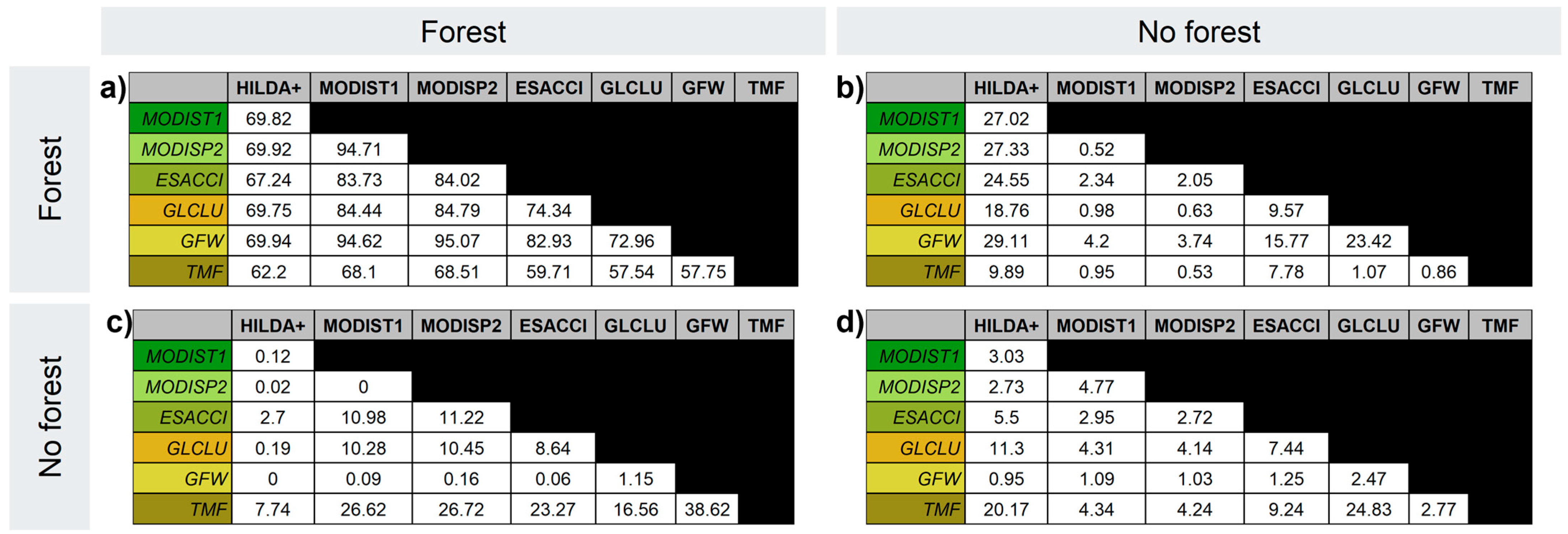
Figure A1. Results of the comparison over the Congo Basin: (a) F/F, (b) NF/F, (c) F/NF, and (d) NF/NF. The cells containing the names of the “compared” datasets are highlighted in different colors, while those containing the “reference” datasets are highlighted in gray.
Forests 16 01609 g0a1
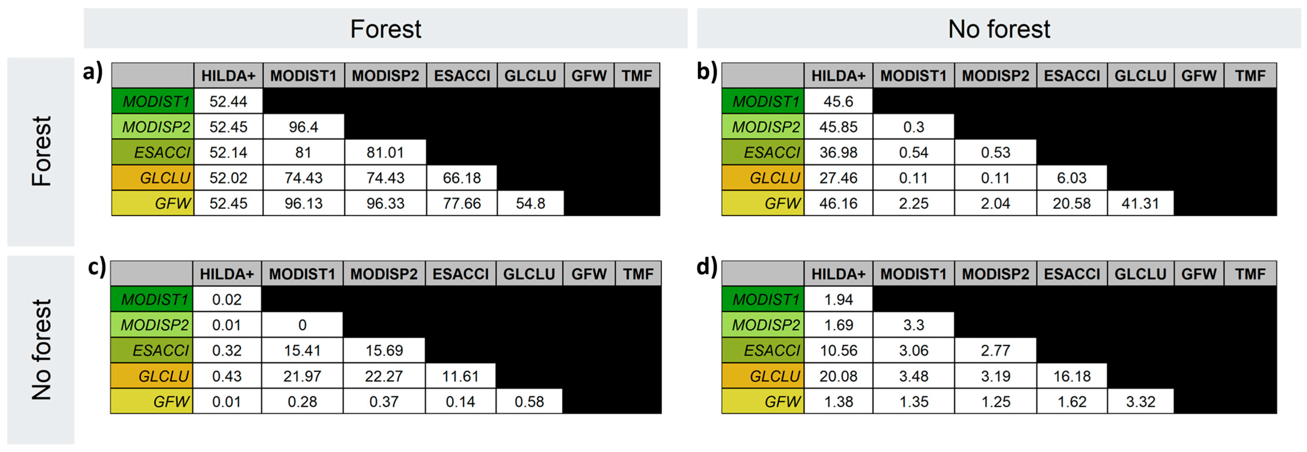
Figure A2. Results of the comparison over the miombo: (a) F/F, (b) NF/F, (c) F/NF, and (d) NF/NF. The cells containing the names of the “compared” datasets are highlighted in different colors, while those containing the “reference” datasets are highlighted in gray.
Forests 16 01609 g0a2
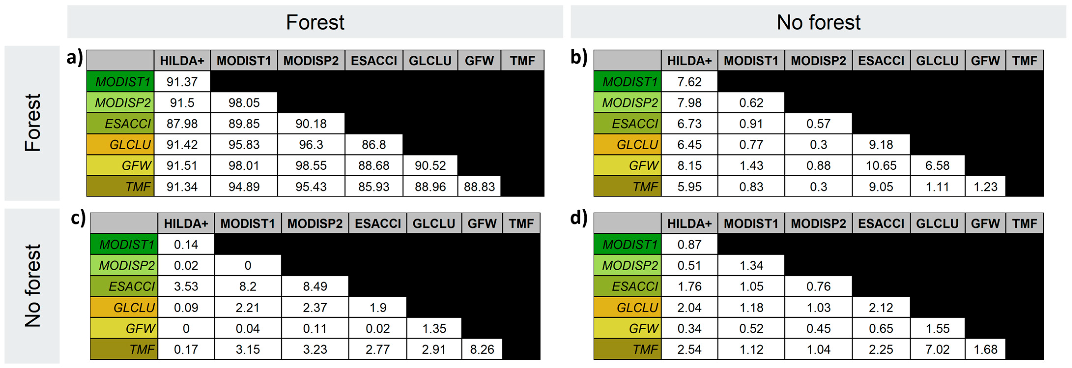
Figure A3. Results of the comparison over the moist forest: (a) F/F, (b) NF/F, (c) F/NF, and (d) NF/NF. The cells containing the names of the “compared” datasets are highlighted in different colors, while those containing the “reference” datasets are highlighted in gray.
Forests 16 01609 g0a3
Figure A4. Results of the comparison over the savanna forest: (a) F/F, (b) NF/F, (c) F/NF, and (d) NF/NF. The cells containing the names of the “compared” datasets are highlighted in different colors, while those containing the “reference” datasets are highlighted in gray.
Forests 16 01609 g0a4
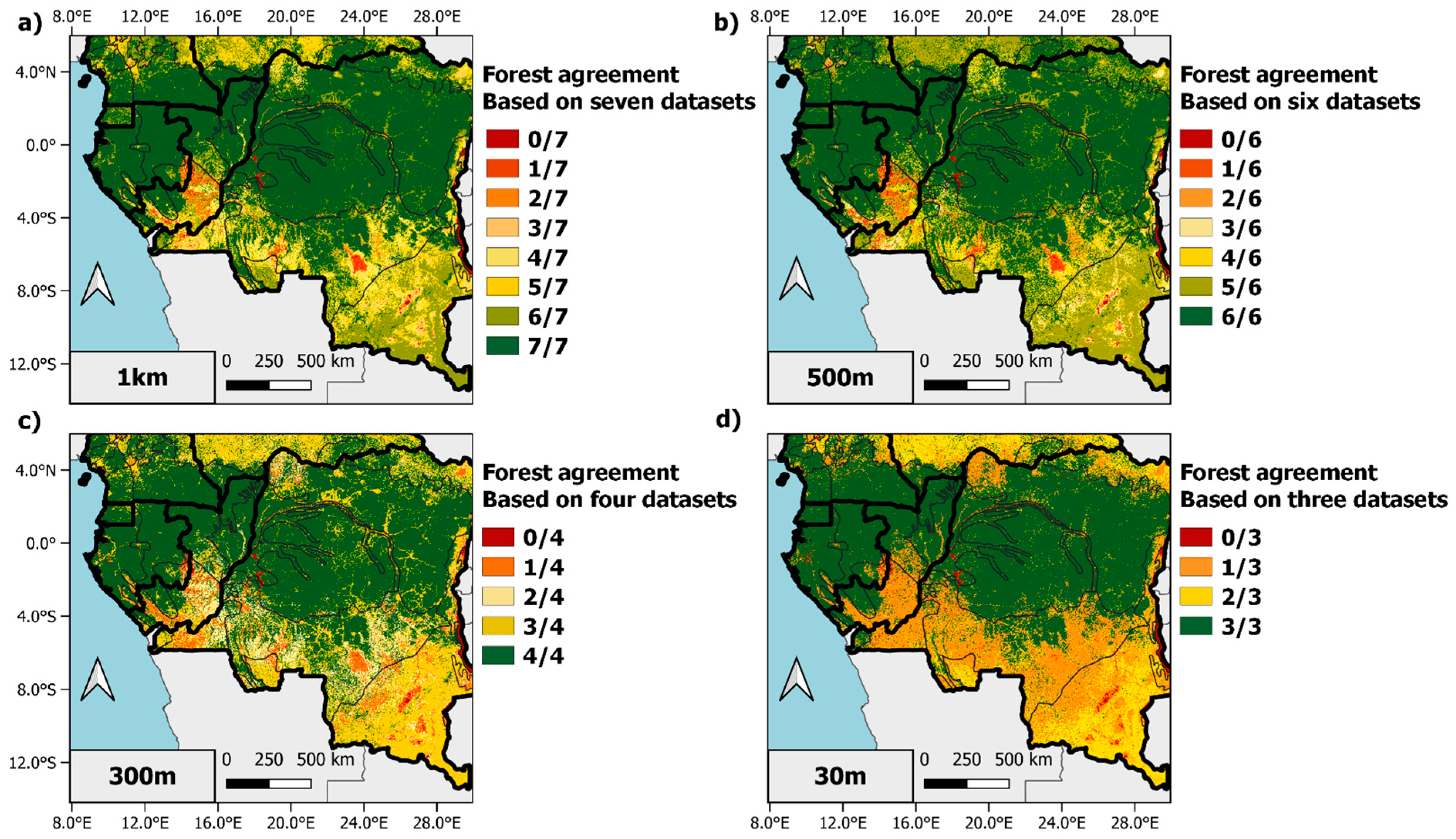
Figure A5. Agreement maps over the Congo Basin. (a) Resolution of 1 km, seven datasets. (b) Resolution of 500 m, six datasets. (c) Resolution of 300 m, four datasets. (d) Resolution of 30 m, three datasets.
Forests 16 01609 g0a5
Figure A6. Maps of forest-cover change from 2001 to 2019 for (a) HILDA+, (b) MODIST1, (c) MODISP2, (d) ESACCI, (e) GLCLU, (f) GFW, and (g) TMF. Pixels in which multiple changes had occurred are in yellow; the ones affected by deforestation (loss) and reforestation (gain) are in red and green, respectively.
Forests 16 01609 g0a6
Figure A7. Number of changes in forest cover observed in the MODIS products. (a) Number of gains for MODIST1. (b) Number of losses for MODIST1. (c) Number of gains for MODISP2. (d) Number of losses for MODISP2. (e) Same results as (ad), but zoomed-in on a small region of the Republic of the Congo.
Forests 16 01609 g0a7
Figure A8. Classes of MODIST1 implicated in the multiple changes.
Forests 16 01609 g0a8
Figure A9. Classes of MODISP2 implicated in the multiple changes.
Forests 16 01609 g0a9

References

  1. Cuni-Sanchez, A.; Sullivan, M.J.P.; Platts, P.J.; Lewis, S.L.; Marchant, R.; Imani, G.; Hubau, W.; Abiem, I.; Adhikari, H.; Albrecht, T.; et al. High Aboveground Carbon Stock of African Tropical Montane Forests. Nature 2021, 596, 536–542. [Google Scholar] [CrossRef]
  2. Spracklen, D.V.; Arnold, S.R.; Taylor, C.M. Observations of Increased Tropical Rainfall Preceded by Air Passage over Forests. Nature 2012, 489, 282–285. [Google Scholar] [CrossRef]
  3. Réjou-Méchain, M.; Mortier, F.; Bastin, J.-F.; Cornu, G.; Barbier, N.; Bayol, N.; Bénédet, F.; Bry, X.; Dauby, G.; Deblauwe, V.; et al. Unveiling African Rainforest Composition and Vulnerability to Global Change. Nature 2021, 593, 90–94. [Google Scholar] [CrossRef]
  4. Hubau, W.; Lewis, S.L.; Phillips, O.L.; Affum-Baffoe, K.; Beeckman, H.; Cuní-Sanchez, A.; Daniels, A.K.; Ewango, C.E.N.; Fauset, S.; Mukinzi, J.M.; et al. Asynchronous Carbon Sink Saturation in African and Amazonian Tropical Forests. Nature 2020, 579, 80–87. [Google Scholar] [CrossRef]
  5. Foley, J.A.; DeFries, R.; Asner, G.P.; Barford, C.; Bonan, G.; Carpenter, S.R.; Chapin, F.S.; Coe, M.T.; Daily, G.C.; Gibbs, H.K.; et al. Global Consequences of Land Use. Science 2005, 309, 570–574. [Google Scholar] [CrossRef] [PubMed]
  6. Curtis, P.G.; Slay, C.M.; Harris, N.L.; Tyukavina, A.; Hansen, M.C. Classifying Drivers of Global Forest Loss. Science 2018, 361, 1108–1111. [Google Scholar] [CrossRef] [PubMed]
  7. Global Forest Resources Assessment 2020; FAO: Rome, Italy, 2020; ISBN 978-92-5-132581-0.
  8. Kissinger, G.; Herold, M.; De sy, V. Drivers of Deforestation and Forest Degradation: A Synthesis Report for REDD+ Policymakers; Lexeme Consulting: Vancouver, BC, Canada, 2012. [Google Scholar]
  9. de Wasseige, C.; Tadoum, M.; Eba’a Atyi, R.; Doumenge, C. (Eds.) Les Forêts du Bassin du Congo: Forêts et Changements Climatiques; Weyrich Édition: Neufchâteau, Belgium, 2015; ISBN 978-2-87489-356-8. [Google Scholar]
  10. Jiang, N.; Li, P.; Feng, Z. Remote Sensing of Swidden Agriculture in the Tropics: A Review. Int. J. Appl. Earth Obs. Geoinf. 2022, 112, 102876. [Google Scholar] [CrossRef]
  11. Gibbs, H.K.; Brown, S.; Niles, J.O.; Foley, J.A. Monitoring and Estimating Tropical Forest Carbon Stocks: Making REDD a Reality. Environ. Res. Lett. 2007, 2, 045023. [Google Scholar] [CrossRef]
  12. Bossy, T.; Ciais, P.; Renaudineau, S.; Wan, L.; Ygorra, B.; Adam, E.; Barbier, N.; Bauters, M.; Delbart, N.; Frappart, F.; et al. State of the Art and for Remote Sensing Monitoring of Carbon Dynamics in African Tropical Forests. Front. Remote Sens. 2025, 6, 1532280. [Google Scholar] [CrossRef]
  13. Chave, J.; Davies, S.J.; Phillips, O.L.; Lewis, S.L.; Sist, P.; Schepaschenko, D.; Armston, J.; Baker, T.R.; Coomes, D.; Disney, M.; et al. Ground Data Are Essential for Biomass Remote Sensing Missions. Surv. Geophys. 2019, 40, 863–880. [Google Scholar] [CrossRef]
  14. Potapov, P.; Hansen, M.C.; Pickens, A.; Hernandez-Serna, A.; Tyukavina, A.; Turubanova, S.; Zalles, V.; Li, X.; Khan, A.; Stolle, F.; et al. The Global 2000-2020 Land Cover and Land Use Change Dataset Derived From the Landsat Archive: First Results. Front. Remote Sens. 2022, 3, 856903. [Google Scholar] [CrossRef]
  15. ESA Land Cover CCI Product User Guide Version 2. Tech. Rep. 2017. Available online: http://maps.elie.ucl.ac.be/CCI/viewer/download/ESACCI-LC-Ph2-PUGv2_2.0.pdf (accessed on 19 February 2025).
  16. Sulla-Menashe, D.; Gray, J.M.; Abercrombie, S.P.; Friedl, M.A. Hierarchical Mapping of Annual Global Land Cover 2001 to Present: The MODIS Collection 6 Land Cover Product. Remote Sens. Environ. 2019, 222, 183–194. [Google Scholar] [CrossRef]
  17. Winkler, K.; Fuchs, R.; Rounsevell, M.; Herold, M. Global Land Use Changes Are Four Times Greater than Previously Estimated. Nat. Commun. 2021, 12, 2501. [Google Scholar] [CrossRef] [PubMed]
  18. Hansen, M.C.; Potapov, P.V.; Moore, R.; Hancher, M.; Turubanova, S.A.; Tyukavina, A.; Thau, D.; Stehman, S.V.; Goetz, S.J.; Loveland, T.R.; et al. High-Resolution Global Maps of 21st-Century Forest Cover Change. Science 2013, 342, 850–853. [Google Scholar] [CrossRef]
  19. Vancutsem, C.; Achard, F.; Pekel, J.-F.; Vieilledent, G.; Carboni, S.; Simonetti, D.; Gallego, J.; Aragão, L.E.O.C.; Nasi, R. Long-Term (1990–2019) Monitoring of Forest Cover Changes in the Humid Tropics. Sci. Adv. 2021, 7, eabe1603. [Google Scholar] [CrossRef]
  20. Ryan, C.M.; Hill, T.; Woollen, E.; Ghee, C.; Mitchard, E.; Cassells, G.; Grace, J.; Woodhouse, I.H.; Williams, M. Quantifying Small-scale Deforestation and Forest Degradation in African Woodlands Using Radar Imagery. Glob. Change Biol. 2012, 18, 243–257. [Google Scholar] [CrossRef]
  21. Mitchard, E.T.A.; Saatchi, S.S.; White, L.J.T.; Abernethy, K.A.; Jeffery, K.J.; Lewis, S.L.; Collins, M.; Lefsky, M.A.; Leal, M.E.; Woodhouse, I.H.; et al. Mapping Tropical Forest Biomass with Radar and Spaceborne LiDAR in Lopé National Park, Gabon: Overcoming Problems of High Biomass and Persistent Cloud. Biogeosciences 2012, 9, 179–191. [Google Scholar] [CrossRef]
  22. Beck, H.E.; Zimmermann, N.E.; McVicar, T.R.; Vergopolan, N.; Berg, A.; Wood, E.F. Present and Future Köppen-Geiger Climate Classification Maps at 1-Km Resolution. Sci. Data 2018, 5, 180214. [Google Scholar] [CrossRef]
  23. Olson, D.M.; Dinerstein, E.; Wikramanayake, E.D.; Burgess, N.D.; Powell, G.V.N.; Underwood, E.C.; D’amico, J.A.; Itoua, I.; Strand, H.E.; Morrison, J.C.; et al. Terrestrial Ecoregions of the World: A New Map of Life on Earth. BioScience 2001, 51, 933. [Google Scholar] [CrossRef]
  24. Martin, E.; Burgess, N. Central Zambezian Wet Miombo Woodlands (AT11) 2020. Available online: https://www.oneearth.org/ecoregions/central-zambezian-wet-miombo-woodlands/ (accessed on 19 February 2025).
  25. Kanschik, W.; Becker, B. Dry Miombo – Ecology of Its Major Plant Species and Their Potential Use as Bio-Indicators. Plant Ecology 2001, 155, 139–146. [Google Scholar] [CrossRef]
  26. Martin, E.; Burgess, N. Central Congolian Lowland Forest (AT14) 2020. Available online: https://www.oneearth.org/ecoregions/central-congolian-lowland-forests/ (accessed on 19 February 2025).
  27. Martin, E.; Burgess, N. Southern Congolian Forest-Savanna (AT13) 2020. Available online: https://www.oneearth.org/ecoregions/southern-congolian-forest-savanna/ (accessed on 19 February 2025).
  28. Burgess, N.D.; D’Amico Hales, J.; Dinerstein, E.; Itoua, I.; Newman, K.; Olson, D.; Ricketts, T.; Schipper, J.; Underwood, E. Terrestrial Ecoregions of Africa and Madagascar: A Conservation Assessment; Island Press: Washington, DC, USA, 2004; ISBN 978-1-55963-364-2. [Google Scholar]
  29. Ogle, S.M.; Sanchez, M.J.S.; Rocha, M.T.; MacDonald, J.D.; Dong, H. IPCC Guidelines for National Greenhouse Gas Inventories, Volume 4 (Agriculture, Forestry and Other Land Use); National Greenhouse Gas Inventories Program; IPCC: Geneva, Switzerland, 2019.
  30. Chazdon, R.L.; Brancalion, P.H.S.; Laestadius, L.; Bennett-Curry, A.; Buckingham, K.; Kumar, C.; Moll-Rocek, J.; Vieira, I.C.G.; Wilson, S.J. When Is a Forest a Forest? Forest Concepts and Definitions in the Era of Forest and Landscape Restoration. Ambio 2016, 45, 538–550. [Google Scholar] [CrossRef]
  31. Tropek, R.; Sedláček, O.; Beck, J.; Keil, P.; Musilová, Z.; Šímová, I.; Storch, D. Comment on “High-Resolution Global Maps of 21st-Century Forest Cover Change”. Science 2014, 344, 981. [Google Scholar] [CrossRef]
  32. Sannier, C.; McRoberts, R.E.; Fichet, L.-V. Suitability of Global Forest Change Data to Report Forest Cover Estimates at National Level in Gabon. Remote Sens. Environ. 2016, 173, 326–338. [Google Scholar] [CrossRef]
  33. Dong, J.; Xiao, X.; Sheldon, S.; Biradar, C.; Zhang, G.; Dinh Duong, N.; Hazarika, M.; Wikantika, K.; Takeuhci, W.; Moore, B. A 50-m Forest Cover Map in Southeast Asia from ALOS/PALSAR and Its Application on Forest Fragmentation Assessment. PLoS ONE 2014, 9, e85801. [Google Scholar] [CrossRef] [PubMed]
  34. Li, W.; Ciais, P.; MacBean, N.; Peng, S.; Defourny, P.; Bontemps, S. Major Forest Changes and Land Cover Transitions Based on Plant Functional Types Derived from the ESA CCI Land Cover Product. Int. J. Appl. Earth Obs. Geoinf. 2016, 47, 30–39. [Google Scholar] [CrossRef]
  35. Liu, A.; Cheng, X.; Chen, Z. Performance Evaluation of GEDI and ICESat-2 Laser Altimeter Data for Terrain and Canopy Height Retrievals. Remote Sens. Environ. 2021, 264, 112571. [Google Scholar] [CrossRef]
  36. Fayad, I.; Baghdadi, N.; Alcarde Alvares, C.; Stape, J.L.; Bailly, J.S.; Scolforo, H.F.; Cegatta, I.R.; Zribi, M.; Le Maire, G. Terrain Slope Effect on Forest Height and Wood Volume Estimation from GEDI Data. Remote Sens. 2021, 13, 2136. [Google Scholar] [CrossRef]
  37. Hamunyela, E.; Brandt, P.; Shirima, D.; Do, H.T.T.; Herold, M.; Roman-Cuesta, R.M. Space-Time Detection of Deforestation, Forest Degradation and Regeneration in Montane Forests of Eastern Tanzania. Int. J. Appl. Earth Obs. Geoinf. 2020, 88, 102063. [Google Scholar] [CrossRef]
  38. Mutanga, O.; Masenyama, A.; Sibanda, M. Spectral Saturation in the Remote Sensing of High-Density Vegetation Traits: A Systematic Review of Progress, Challenges, and Prospects. ISPRS J. Photogramm. Remote Sens. 2023, 198, 297–309. [Google Scholar] [CrossRef]
  39. Joshi, N.; Mitchard, E.T.A.; Brolly, M.; Schumacher, J.; Fernández-Landa, A.; Johannsen, V.K.; Marchamalo, M.; Fensholt, R. Understanding ‘Saturation’ of Radar Signals over Forests. Sci. Rep. 2017, 7, 3505. [Google Scholar] [CrossRef]
  40. Melo, J.B.; Ziv, G.; Baker, T.R.; Carreiras, J.M.B.; Pearson, T.R.H.; Vasconcelos, M.J. Striking Divergences in Earth Observation Products May Limit Their Use for REDD+. Environ. Res. Lett. 2018, 13, 104020. [Google Scholar] [CrossRef]
  41. Hakkenberg, C.R.; Atkins, J.W.; Brodie, J.F.; Burns, P.; Cushman, S.; Jantz, P.; Kaszta, Z.; Quinn, C.A.; Rose, M.D.; Goetz, S.J. Inferring Alpha, Beta, and Gamma Plant Diversity across Biomes with GEDI Spaceborne Lidar. Environ. Res. Ecol. 2023, 2, 035005. [Google Scholar] [CrossRef]
  42. Reiche, J.; Mullissa, A.; Slagter, B.; Gou, Y.; Tsendbazar, N.-E.; Odongo-Braun, C.; Vollrath, A.; Weisse, M.J.; Stolle, F.; Pickens, A.; et al. Forest Disturbance Alerts for the Congo Basin Using Sentinel-1. Environ. Res. Lett. 2021, 16, 024005. [Google Scholar] [CrossRef]
  43. Torresani, M.; Rocchini, D.; Alberti, A.; Moudrý, V.; Heym, M.; Thouverai, E.; Kacic, P.; Tomelleri, E. LiDAR GEDI Derived Tree Canopy Height Heterogeneity Reveals Patterns of Biodiversity in Forest Ecosystems. Ecol. Inform. 2023, 76, 102082. [Google Scholar] [CrossRef] [PubMed]
  44. Ygorra, B.; Frappart, F.; Wigneron, J.P.; Moisy, C.; Catry, T.; Baup, F.; Hamunyela, E.; Riazanoff, S. Monitoring Loss of Tropical Forest Cover from Sentinel-1 Time-Series: A CuSum-Based Approach. Int. J. Appl. Earth Obs. Geoinf. 2021, 103, 102532. [Google Scholar] [CrossRef]
  45. Ygorra, B.; Frappart, F.; Wigneron, J.-P.; Catry, T.; Pillot, B.; Pfefer, A.; Courtalon, J.; Riazanoff, S. A Near-Real-Time Tropical Deforestation Monitoring Algorithm Based on the CuSum Change Detection Method. Front. Remote Sens. 2024, 5, 1416550. [Google Scholar] [CrossRef]
  46. Reiche, J.; Hamunyela, E.; Verbesselt, J.; Hoekman, D.; Herold, M. Improving Near-Real Time Deforestation Monitoring in Tropical Dry Forests by Combining Dense Sentinel-1 Time Series with Landsat and ALOS-2 PALSAR-2. Remote Sens. Environ. 2018, 204, 147–161. [Google Scholar] [CrossRef]
  47. Potapov, P.; Li, X.; Hernandez-Serna, A.; Tyukavina, A.; Hansen, M.C.; Kommareddy, A.; Pickens, A.; Turubanova, S.; Tang, H.; Silva, C.E.; et al. Mapping Global Forest Canopy Height through Integration of GEDI and Landsat Data. Remote Sens. Environ. 2021, 253, 112165. [Google Scholar] [CrossRef]
  48. Lang, N.; Jetz, W.; Schindler, K.; Wegner, J.D. A High-Resolution Canopy Height Model of the Earth. Nat. Ecol. Evol. 2023, 7, 1778–1789. [Google Scholar] [CrossRef]
  49. Fayad, I.; Ciais, P.; Schwartz, M.; Wigneron, J.-P.; Baghdadi, N.; De Truchis, A.; d’Aspremont, A.; Frappart, F.; Saatchi, S.; Sean, E.; et al. Hy-TeC: A Hybrid Vision Transformer Model for High-Resolution and Large-Scale Mapping of Canopy Height. Remote Sens. Environ. 2024, 302, 113945. [Google Scholar] [CrossRef]
  50. Sollier, V.; Frappart, F.; Bourrel, L.; Couvreur, T.L.P.; Peaucelle, M.; Renaudineau, S.; Huaraca, L.; Wigneron, J.-P. Long-Term Evolution of Forest Cover in the Pacific Coast of Ecuador (1960–2019): A Comparison of Land Use/Land Cover (LULC) Remote Sensing Products. Front. Remote Sens. 2025, 6, 1536105. [Google Scholar] [CrossRef]
  51. Sankaran, M.; Hanan, N.P.; Scholes, R.J.; Ratnam, J.; Augustine, D.J.; Cade, B.S.; Gignoux, J.; Higgins, S.I.; Le Roux, X.; Ludwig, F.; et al. Determinants of Woody Cover in African Savannas. Nature 2005, 438, 846–849. [Google Scholar] [CrossRef] [PubMed]
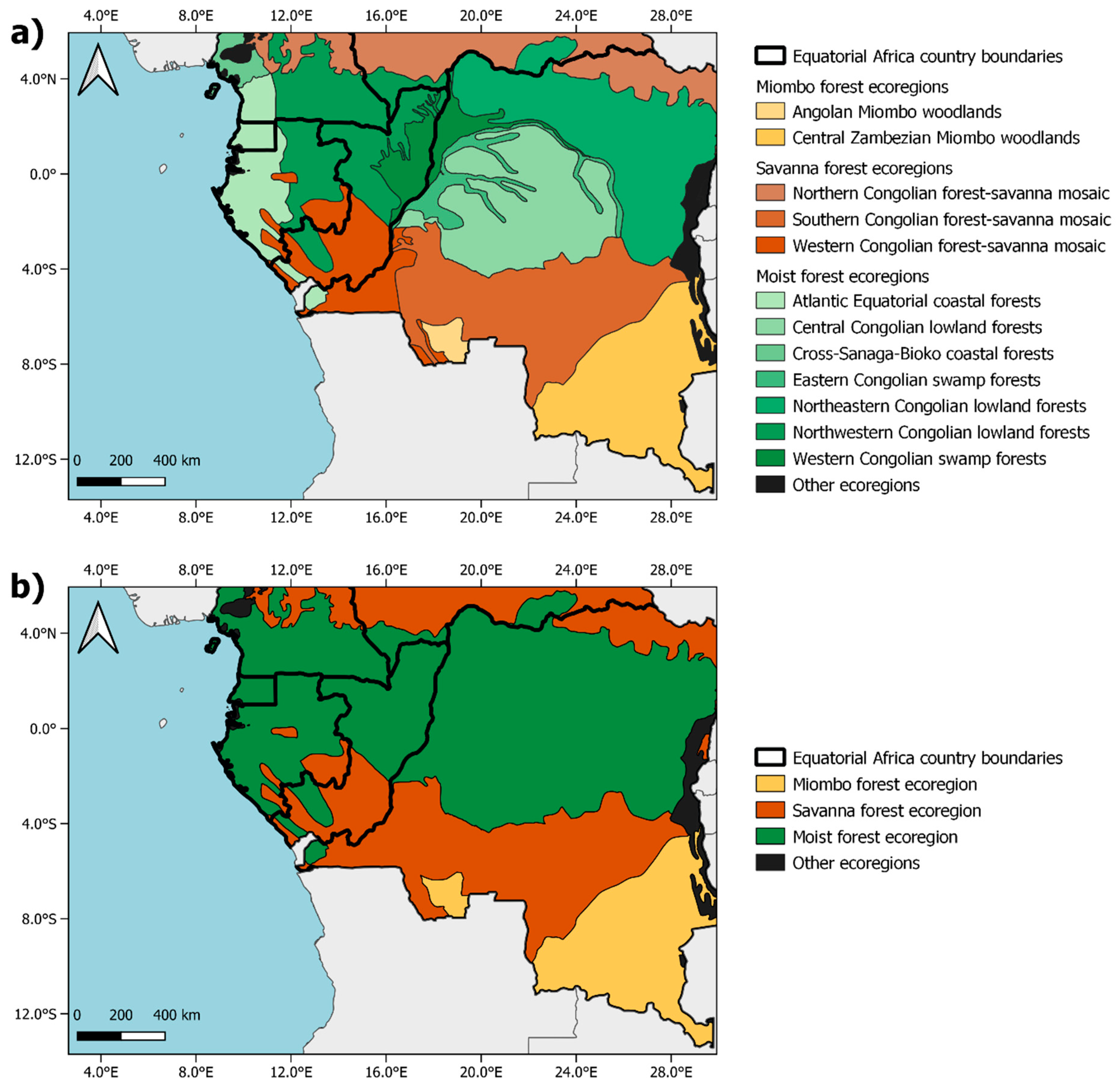
Figure 1. Map of the studied areas across the Congo Basin. (a) Ecoregions of the Terrestrial Ecoregions of the World (TEOW). (b) Ecoregions studied are miombo, savanna, and moist forest.
Forests 16 01609 g001
Figure 2. Representation of the methodology used to compare the datasets. The (first step) corresponds to the dataset-resolution change. The (second step) corresponds to the production of the comparison map. The (third step) corresponds to the extraction of the LULC classes from the “reference” map.
Forests 16 01609 g002
Figure 3. Forest/non-forest mask for each dataset on the studied area, at their initial resolution. (a) GFW, (b) ESACCI, (c) TMF, (d) MODIST1, (e) GLCLU, (f) MODISP2, and (g) HILDA+ for the year 2005.
Forests 16 01609 g003
Figure 4. Forest/non-forest mask for each dataset at every resolution. (a) TMF, (b) GFW, (c) GLCLU, (d) ESACCI, (e) MODISP2, (f) MODIST1, and (g) HILDA+ at each resolution for the year 2005.
Forests 16 01609 g004
Figure 5. Agreement and disagreement rate for the databases, expressed in the percentage of the mean area (2005, 2010, and 2015) over the Congo Basin and three ecoregions. Colored cells correspond to the “compared” datasets. Gray cells correspond to the “reference” dataset. (a) Agreement over the Congo Basin. (b) Disagreement over the Congo Basin. (c) Agreement over the miombo. (d) Disagreement over the miombo. (e) Agreement over the moist forest. (f) Disagreement over the moist forest. (g) Agreement over the savanna. (h) Disagreement over the savanna.
Forests 16 01609 g005
Figure 6. LULC classes implicated in the NF/F disagreements between the different datasets. (a) Results for the Congo Basin. (b) Results for the miombo. (c) Results for the moist forest. (d) Results for the savanna.
Forests 16 01609 g006
Figure 7. Maps of forest-cover change from 2001 to 2019 for (a) GFW, (b) ESACCI, (c) TMF, (d) MODIST1, (e) GLCLU, (f) MODISP2, and (g) HILDA+. Pixels in which multiple changes occurred are in yellow; the pixels affected by deforestation (loss) and reforestation (gain) are in red and green, respectively.
Forests 16 01609 g007
Figure 8. Cumulative sum of the area of net forest change between 2001 and 2019 for (a) the Congo Basin, (b) miombo forest, (c) moist forest, and (d) savanna forest.
Forests 16 01609 g008
Table 1. Summary of the datasets used in the intercomparison study, along with their main characteristics. The characteristics include spatial resolution, temporal resolution, temporal coverage, sensors, classification methodology, and number of classes.
HILDA+MODIST1MODISP2ESACCIGLCLUGFWTMF
Spatial resolution1000 m500 m500 m300 m30 m30 m30 m
Temporal resolution AnnualAnnualAnnualAnnualEvery 5 yearsAnnualAnnual
Temporal coverage1960–20192001–20222001–20221992–20202000–20202000–20221990–2022
SensorsMulti-sourceMODISMODISAVHRR, MERIS, SPOT-VGT, PROBA-V, S3-OLCILandsat
GEDI
LandsatLandsat
Classification methodologySupervisedSupervisedSupervisedUnsupervisedSupervisedSupervisedSupervised
Number of classes6181236110Continuous tree cover between 0 and 100%
Year of forest loss
6
Table 2. Forest and non-forest area percentage of all the datasets at each resolution and for each studied area.
Congo BasinMiomboMoist forestSavanna
DatasetNon-Forest
Percentage
Forest
Percentage
Non-Forest PercentageForest
Percentage
Non-Forest PercentageForest
Percentage
Non-Forest PercentageForest
Percentage
Resolution
HILDA+30.1669.8447.8952.118.5491.4656.0443.961 km
MODIST13.1696.841.9698.041.0198.995.7094.301 km
MODISP22.7597.251.7098.300.5399.475.6294.381 km
ESACCI8.2091.8010.8889.125.2994.719.4690.541 km
GLCLU11.4988.5120.5179.492.1397.8721.7578.251 km
GFW0.9599.051.3998.610.3599.650.6899.321 km
TMF27.9172.09 2.7197.2942.7457.261 km
MODIST15.2994.713.6096.401.9598.059.6990.31500 m
MODISP24.7795.233.3096.701.3498.669.5390.47500 m
ESACCI13.9386.0718.4681.549.2590.7517.1282.88500 m
GLCLU14.5885.4225.4674.543.4096.6027.0572.95500 m
GFW1.1898.821.6398.370.5699.440.9199.09500 m
TMF30.9669.04 4.2795.7349.3150.69500 m
ESACCI17.0282.9822.2077.8011.3088.7021.5578.45300 m
GLCLU16.0983.9127.7972.214.0295.9829.6370.37300 m
GFW1.3098.701.7698.240.6799.331.0398.97300 m
TMF32.5167.49 5.0294.9852.6547.35300 m
GLCLU25.9074.1044.6355.378.1391.8745.4254.5830 m
GFW3.6396.373.9096.102.9097.103.5096.5030 m
TMF41.4058.60 9.9490.0669.5430.4630 m
Disclaimer/Publisher’s Note: The statements, opinions and data contained in all publications are solely those of the individual author(s) and contributor(s) and not of MDPI and/or the editor(s). MDPI and/or the editor(s) disclaim responsibility for any injury to people or property resulting from any ideas, methods, instructions or products referred to in the content.