Abstract
The flat peach, an important commercial crop in the 143rd Regiment of Shihezi, China, is overwintered using plastic film mulching. Flat peaches are cultivated to boost the local temperate rural economy. The development of accurate maps of the spatial distribution of flat peach plantations is crucial for the intelligent management of economic orchards. This study evaluated the performance of pixel-based and object-based random forest algorithms for mapping flat peaches using the GF-1 image acquired during the overwintering period. A total of 45 variables, including spectral bands, vegetation indices, and texture, were used as input features. To assess the importance of different features on classification accuracy, the five different sets of variables (5, 15, 25, and 35 input variables and all 45 variables) were classified using pixel/object-based classification methods. Results of the feature optimization suggested that vegetation indices played a key role in the study, and the mean and variance of Gray-Level Co-occurrence Matrix (GLCM) texture features were important variables for distinguishing flat peach orchards. The object-based classification method was superior to the pixel-based classification method with statistically significant differences. The optimal performance was achieved by the object-based method using 25 input variables, with an overall accuracy of 94.47% and a Kappa coefficient of 0.9273. Furthermore, there were no statistically significant differences between the image-derived flat peach cultivated area and the statistical yearbook data. The result indicated that high-resolution images based on the overwintering period can successfully achieve the mapping of flat peach planting areas, which will provide a useful reference for temperate lands with similar agricultural management.
1. Introduction
The flat peach, originally from Xinjiang, China [1], was introduced and cultivated in Japan, Europe, and America in the 17th century [2]. It plays a very important role in temperate rural economic development [3]. Benefiting from its unique natural environment, Xinjiang’s flat peaches are renowned both domestically and internationally for their delicious taste and fine texture [4]. In October 2000, the 143rd Regiment of Shihezi City, the largest flat peach planting base in Xinjiang, was officially named ‘The Hometown of Chinese Flat Peaches’ by the China Specialty Agricultural Products Committee. Currently, the flat peach industry has become a distinctive sector of the regiment and an important source of income for growers [5]. Although information on flat peach cultivation is of great practical importance, existing data is limited to statistical data, and there has been no research on the spatial distribution of flat peaches. Therefore, an approach based on the overwintering period for mapping flat peaches was developed in this study, aiming to improve the refined and intelligent management of flat peaches.
The traditional methods, such as hierarchical reporting and statistical sampling, are widely adopted in crop area information acquisition, but they are time-consuming, labor-intensive and difficult to obtain accurate spatial distribution information [6]. Remote sensing technology, with its characteristics of rapid and large-scale monitoring of agricultural information, has been widely used in monitoring crop planting areas and spatial distribution [7,8]. Medium and low-resolution remote sensing images such as Sentinel [9,10], Landsat [11,12,13], and MODIS [11,14,15] are relatively easy to obtain and cost-effective, commonly used for large-scale, multi-temporal crop remote sensing identification. However, the selection of images is related to the spatial scale of the target features [16]. The flat peach orchard plots in Shihezi are small and fragmented, making the application of medium and low-resolution image data more limited and difficult to meet the requirements for extracting refined planting information. The advantages of high-resolution remote sensing data make it possible to effectively overcome issues such as the fragmentation of planting areas and small plots. Since the launch of China’s GF-1 satellite, it has demonstrated significant potential for agricultural monitoring. For example, Luo et al. [17] successfully achieved detailed mapping of mango plantations in tropical regions using GF-1/PMS data.
At present, there are two main methods for crop mapping using remote sensing data. The first classification method is based on time-series remote sensing images to reflect the changes in crop growth over time, thereby extracting phenological indicators for model input [6,18,19,20]. However, the effectiveness of this method is related to the design of time series data, which is typically large in volume and complex to process [21,22]. The second classification method is based on phenological differences, selecting specific time windows for land cover classification. This approach not only achieves good classification results but also significantly reduces computational costs and improves classification efficiency. Xu et al. [23] conducted land use classification in a mining-agricultural composite area based on single-temporal Landsat images, achieving a classification accuracy of 92.38%. Wei et al. [24] used single-temporal images combined with vector data for classification, with accuracy higher than that of dual-temporal image classification. This method requires that the target land cover type in the critical time window can be clearly distinguished from other land cover types to facilitate remote sensing identification. Most existing crop mapping based on specific phenological times is concentrated in the growing season, such as rice mapping with obvious flooding signals [25], cotton planting mapping using the cotton budding period [26], and accurate canola mapping based on the flowering period [27]. However, there has been no research using overwintering period imagery for orchard mapping. In the study area, flat peaches are overwintered by covering them with straw mats and plastic film, with the overwintering period lasting from mid-October to April of the following year [28]. In March, snow and ice gradually melt, vegetation cover is sparse, and the surface structure becomes clearer. Existing research has shown that white agricultural plastic film can enhance surface reflection [29]. Therefore, this study used high-resolution data from this period to explore whether accurate mapping of flat peach planting can be achieved.
Crop classification methods can be divided into pixel-based methods and object-based methods according to the basic units of classification. Many scholars found that object-based methods typically outperform pixel-based methods when comparing the classification accuracy from agriculture to other land cover categories [30,31]. With the development of machine learning, popular machine learning algorithms have been widely used for crop identification including Maximum Likelihood Classification (MLC) [32], Decision Tree (DT) [33], Artificial Neural Networks (ANN) [34], Support Vector Machine (SVM) [17], and Random Forest (RF) [35]. Among them, RF has demonstrated robustness and accuracy in multiple mapping studies [36,37]. The comparative analysis of pixel-based and object-based random forest algorithms has been conducted for mapping wetland vegetation [38], mangrove forests [39], and agricultural landscapes [40]. However, there has been lack of comparison of pixel-based with object-based image analysis using the GF-1 data for mapping flat peaches.
As shown above, the objectives of this research are threefold: (1) to evaluate the capabilities of pixel-based and object-based RF algorithms for flat peach plantation mapping; (2) to explore the importance of different types of Supplementary Information (spectral bands, vegetation indices, and textural features) to identify flat peach plantations; and (3) to explore the potential of the using GF-1 imagery and winter plastic film signals to separate flat peach orchards from other ground covers.
2. Materials and Methods
Based on GF-1/PMS remote sensing images during the overwintering period, spectral, vegetation index, and texture features were extracted in this study. According to the importance order of feature variables, five different sets of variables were formed. The pixel-based and object-based RF algorithm was used to map the planting area of flat peaches in the 143rd Regiment of Shihezi. Through statistical data and confusion matrix, the impact of different schemes on the classification results of flat peaches was analyzed, aiming to determine the most suitable classification method for the information extraction of flat peaches. The main research ideas of this study are shown in Figure 1.
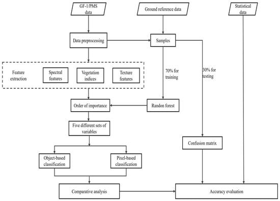
Figure 1.
The workflow for mapping flat peaches by GF-1 data.
2.1. Study Area
The study area is located in the northern part of the 143rd Regiment of the 8th Division of the Xinjiang Production and Construction Corps (44°12′–44°29′ N, 85°30′–85°58′ E), mainly including 19 agricultural companies such as the 4th Company, 7th Company, 9th Company, 10th Company, and Nongyi Company, with a total area of approximately 228.37 km2. The study area is situated on the northern slope of the Tianshan Mountains, at the southern edge of the Junggar Basin, with an average altitude of 595 m, an annual average temperature of 6.7 °C, an annual effective accumulated temperature of ≥10 °C ranging from 3650 to 3900 °C, and a frost-free period of 135–191 days, belonging to a mid-temperate continental arid climate. The area experiences cold winters, hot summers, dry and rainless conditions, a long frost-free period, moderate heat, abundant sunshine, evaporation exceeding precipitation, significant annual and daily temperature differences. All the climatic conditions are suitable for the growth and sugar accumulation of flat peaches. The location of the study area is shown in Figure 2.
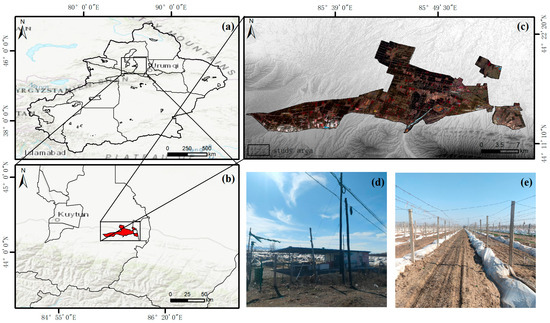
Figure 2.
(a,b) The location of the study area in Xinjiang; (c) GF-1 false color image of the study area; (d) flat peaches during the overwintering period; (e) grapes during the overwintering period.
2.2. Remote Sensing Image Data Acquisition and Preprocessing
The GF-1 satellite is the first satellite of the space-based system in China’s major project of high-resolution earth observation project. The GF-1/PMS image data (GF1B_PMS_E85.7_N44.1_20210323_L1A1227953949) from 23 March 2021, used in this study, was downloaded from the China Centre for Resources Satellite Data and Application (https://data.cresda.cn/#/home, accessed on 16 April 2024). The GF-1/PMS includes 2 m resolution panchromatic and 8 m resolution multispectral (blue, green, red, and near-infrared bands) data. Detailed parameters of the satellite are listed in Table 1.

Table 1.
Band Characteristics and Spatial Resolution of GF-1/PMS.
This study utilized ENVI 5.6 software to preprocess the image, including radiometric calibration, atmospheric correction, orthorectification, and image fusion. The digital number (DN) values of the image were converted to radiance values based on the calibration coefficients provided by the China Center for Resources Satellite Data and Application. To eliminate interference from atmospheric factors, the FLAASH atmospheric correction model was used to convert the radiance of multispectral data into surface reflectance data. Based on ASTER GDEM V3 data and the RPC parameters of the image, orthorectification was performed on both panchromatic and multispectral data. Subsequently, the Nearest Neighbor Diffusion (NNDiffuse) Pan Sharpening image fusion algorithm was employed to fuse the panchromatic and multispectral data, generating a new image with high spatial resolution and multispectral information.
2.3. Field Observations and Statistical Data
This study conducted field surveys in the research area on 7 April 2024. The main field crops in the research area are winter wheat, corn, and cotton, with flat peaches and grapes being the primary fruit trees, along with some vegetables. The study selected the imaging time in late March, when most fields were fallow, some fields were planted with winter wheat, and grapes and flat peaches were in the overwintering period. Grapes and flat peaches covered with plastic film were easily visually identified in field surveys and satellite images. Therefore, the main land cover types in the research area were classified into six categories: flat peach, grape, cropland (winter wheat and fallow land), forest, construction land (buildings and roads), and water. Using a handheld Global Positioning System (GPS), 213 flat peach measurement points and 41 grape measurement points were obtained in the research area. Since the acquisition time of the measured data was later than the imaging time, we used the distance metric method [41], calculating the cosine similarity of the measured points (254 points) for flat peaches and grapes in 2021 and 2024 to assess whether the sample points had changed. Specifically, based on the Google Earth Engine (GEE) platform, we obtained all available Sentinel-2 images with cloud coverage below 10% between 1 April and 1 October for two different years. We selected B2, B3, B4, B5, B6, B7, B8, B8A, B11, and B12 bands of the images for median compositing, and considered sample points with a similarity threshold below 0.2 as ‘unchanged’. After calculation, we found that 251 sample points remained “unchanged” between 2021 and 2024, and the geographical information of the “changed” samples is shown in Table S1. Thus, the high spectral similarity (above 98%) proved that the measured samples from 2024 could be used for the classification task of 2021. Based on prior knowledge and the Google Earth platform, sample information for each land cover type was collected through visual interpretation on the fused images, resulting in a total of 1635 sample points. These samples were then randomly divided into a training sample set and a validation sample set in a 7:3 ratio. Table 2 shows the number of sample points for each land cover type. Figure S1 shows the spatial distribution of the training and validation samples. The 2021 flat peach planting area statistics for the research area were obtained from the ‘2022 Xinjiang Production and Construction Corps Statistical Yearbook’ and were used to evaluate the mapping accuracy of the 2021 flat peach planting.
Table 2.
Land Cover Types and Their Sample Size.
2.4. Multi-Scale Segmentation
Image segmentation is the core step of object-based classification. It is the process of dividing the entire image into several sub-regions with similar ground feature information based on certain homogeneity or heterogeneity conditions, such as grayscale features, texture features, and shape features. In this study, the segmentation process was achieved through multi-scale segmentation in eCognition 9.0 software, which is a bottom-up technique that gradually merges image pixels into a regional object. This process requires setting three key parameters: segmentation scale, shape, and compactness [42]. The selection of the scale parameter directly affects the quality and accuracy of the final image analysis. A segmentation scale that is too large will blur the edge information of the object, while a segmentation scale that is too small will fragment the image details. The total weight of the shape factor and the spectral factor is 1, which affects the overall heterogeneity of the image object. The shape factor includes smoothness and compactness, and the consistency of the internal spectrum of the image object is controlled by setting the weight of the shape factor. To select an appropriate scale parameter, we combined the ESP tool [43] (Figure S2) and tested different scales from 10 to 250, at intervals of 10, for their ability to identify flat peach orchards. We ultimately set the scale parameter to 110, and the compactness and shape factors to 0.5 and 0.6, respectively. Figure S3 shows the three scale levels of 80, 110, and 140. When the scale was 80, the uniform flat peach plots were divided into multiple objects. When the scale was 140, the flat peach objects contained other heterogeneous components.
2.5. Feature Selection
The combination of multiple feature variables is an effective means to improve the classification accuracy of remote sensing images. This study used 45 feature variables, including original bands, vegetation indices, and texture features, for model training. The original bands are the average spectral reflectance of four bands: Blue, Green, Red, and NIR. The vegetation indices include nine indices: Simple Ratio Index (SRI) [17], Green Vegetation Index (VIgreen) [17], Normalized Difference Vegetative Index (NDVI) [36], Renormalized Difference Vegetation Index (RDVI) [17], Modified Simple Ratio (MSR) [44], Soil Adjusted Vegetation Index (SAVI) [45], Difference Vegetation Index (DVI) [35], Enhanced Vegetation Index (EVI) [6], and Red Green Ratio Index (RG) [46]. In high spatial resolution images, the texture information of different objects is particularly evident. The texture features used in this study are based on the Gray-Level Co-occurrence Matrix (GLCM) and include eight texture statistics: Mean, Variance, Entropy, Angular Second Moment, Homogeneity, Contrast, Dissimilarity, and Correlation. The calculation formulas for the feature variables are shown in Table 3.
Table 3.
Description of feature variables.
2.6. Random Forest Algorithm
The Random Forest (RF) algorithm, proposed by Breiman in 2001, is an ensemble machine learning algorithm based on decision trees [47]. It is widely used in crop classification and land cover mapping [36,48,49]. The final prediction result of Random Forest is determined by majority voting from multiple independent decision trees. During the model training process, the interference of outliers and noise is effectively reduced by using the Bagging (Bootstrap Aggregating) algorithm, and it has good processing capability for high-dimensional data. The higher the accuracy of the random forest model, the higher the mapping accuracy of the flat peach. In the RF model construction process, two parameters need to be adjusted, namely the number of decision trees () and the number of features considered when splitting nodes in each tree (). In this study, is set to the square root of the total number of input features [38]. 45 feature variables of GF-1 image data were input, with set to 6. Out-of-bag samples (OOB, samples not selected when constructing a single decision tree) account for approximately 1/3 of all training data. By calculating the OOB error (, the difference between the observed and predicted values of out-of-bag data), the model performance and the importance of feature variables can be evaluated. To evaluate the impact of the parameter on classification accuracy, the out-of-bag accuracy was tested for ranging from 0 to 500. As shown in Figure 3, the OOB accuracy increases with the increase of , and stabilizes when exceeds 150. When the number of trees approaches 500, the model’s accuracy difference is within 1%. Considering the computational time cost of RF, this study sets to 150.
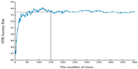
Figure 3.
The impact of Ntree parameters on the accuracy (OOB accuracy rate) of random forest classifiers.
Feature optimization is crucial for image classification, as it can enhance model performance by removing redundant information. This study performed feature selection using the Random Forest algorithm. The importance of each feature () was assessed by measuring the increase in after its random permutation. If the increases significantly, it indicates that the feature is important. The importance (VI) of feature is calculated using the following formula:
Based on the ranking of feature variable importance, five different sets of variables were set up for comparative study to explore the best scheme for improving the mapping accuracy of flat peach planting and to investigate the impact of feature variables on the mapping accuracy of flat peach planting. The corresponding number of features for the five classification schemes are 5, 15, 25, 35, and 45, respectively.
The window size will directly affect the amount of information in the feature vector extracted by GLCM. This study utilized ENVI 5.6 to obtain the GLCM texture information of GF-1/PMS image under six different window sizes: 3 × 3, 5 × 5, 7 × 7, 9 × 9, 11 × 11, and 13 × 13. The random forest algorithm was used to classify the texture features of the six window sizes. By analyzing the classification accuracy under different window sizes in the 45° direction, it was found that the classification accuracy was the highest when the window size was 9 × 9. When we input the texture features using the 45° direction and the average texture features of the 0°, 45°, 90°, and 135° directions in the 9 × 9 window into the random forest model, we found that the latter had a 2% higher classification accuracy than the former. Therefore, this study selected the GLCM texture features of the mean values in the four directions within the 9 × 9 window for subsequent research [17].
2.7. Accuracy Evaluation
This study used a confusion matrix and McNemar’s test to evaluate the accuracy between different classification methods. The following metrics were adopted to assess classification accuracy: Overall Accuracy (OA), Producer Accuracy (PA), User Accuracy (UA), the Kappa coefficient, F1 score [17,50,51], and Intersection over Union (IoU) [52]. McNemar’s test was used to evaluate whether there is a statistical difference between two classifications [40,53]. The formula is as follows:
where represents the number of samples correctly classified by type 1 and incorrectly classified by type 2, and shows the number of samples correctly classified by type 2 and incorrectly classified by type 1. If |z| > 1.96, it indicates that the difference between the two classifications is statistically significant.
3. Results
3.1. Feature Variable Importance Analysis
As shown in Figure 4, the important scores are ranked from high to low. RG was the most critical feature affecting classification, and VIgreen, SRI, and EVI also showed high importance, indicating that vegetation indices have a significant impact on classification accuracy. The overall importance of the original band features was secondary to the vegetation indices, but they played an important role in classification, indicating that the spectral information of the image can effectively reflect the characteristics of various ground objects. Among the texture features, B1_Var showed the highest importance, followed by B1_Mean, B3_Var, B2_Mean, etc. Overall, the importance of GLCM texture features, from high to low, was Var, Mean, Cor, Hom, Ent, Asm, Con, and Dis.
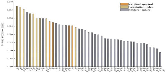
Figure 4.
Feature variable importance ranking.
3.2. Analysis of Partial Extraction Results in the Study Area
For the five feature combination classification schemes, pixel-based and object-based random forest classifications were conducted to obtain the spatial planting structure of various land cover types in the study area. The classification results of some concentrated flat peach planting areas were randomly selected for detailed display and compared with the false-color original image data (Figure 5 and Figure 6). The flat peach planting structure extracted based on the method in this study basically matches the actual distribution.
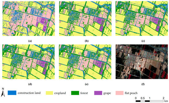
Figure 5.
Comparison of pixel-based classifications: (a–e) show the local detail mapping using 5, 15, 25, 35 and 45 input variables, respectively; (f) is the corresponding false color original image.
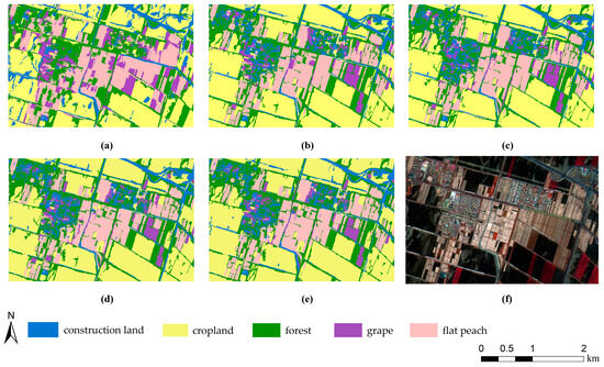
Figure 6.
Comparison of object-based classifications: (a–e) show the local detail mapping using 5, 15, 25, 35 and 45 input variables, respectively; (f) is the corresponding false color original image.
As shown in Figure 5 and Figure 6, the distribution of land cover types divided by the two classification methods was roughly the same, with cropland showing a blocky distribution, while flat peaches, grapes, forest, and construction land exhibit an interleaved distribution. As the number of features increases, the overall classification results of Schemes 2–5 (Figure 5b–e and Figure 6b–e) did not change significantly. However, from Scheme 1 (Figure 5a and Figure 6a) to Scheme 2 (Figure 5b and Figure 6b), it can be observed that the classification effectiveness of various land cover types had greatly improved, indicating that adding 4 vegetation indices, 4 texture features, and 2 original bands on the basis of RG, VIgreen, SRI, B1_Var, and EVI was very useful for improving the classification accuracy of various land cover types. By comparing the classification results of the two methods, it was found that the pixel-based extraction results are more fragmented, and flat peaches were severely confused with forest, buildings, and grapes. On the other hand, the object-based classification method can effectively avoid the ‘Salt and pepper noise’, and the extraction results of flat peach plots were more complete, although there was still some misclassification between grapes, flat peaches, forest, and buildings. Visually, the object-based classification method was superior to the pixel-based method, indicating that the object-based classification method outperformed the pixel-based method in the extraction of flat peach planting areas from high-resolution images, providing better classification results.
3.3. Comparison of Pixel-Based and Object-Based RF Classification Accuracies
Table 4 displays the overall accuracies for the five classification schemes. The accuracy confusion matrix based on pixel and object-based classification methods is shown in Table S2. Except for Scheme 1, the OA and Kappa coefficient of object-based classification were higher than those of pixel- based classification. As the number of features increased from 5 to 25, the OA of object-based classification increased by 22.34%, while the OA of pixel-based classification increased by 11.70%. The above indicated that the responses of object-based and pixel-based classifications to the feature set are inconsistent, and the first 25 feature variables had a greater impact on object-based classification.
Table 4.
The classification accuracy of different schemes.
The McNemar’s test showed that, except for Scheme 2, the difference between object-based and pixel-based classifications was statistically significant (Table 5). When comparing object-based classifications, the difference between Scheme 1 and other schemes was statistically significant, and the difference in classification accuracy between Scheme 2 and Scheme 3 was significant. Among pixel-based schemes, there was also a statistically significant difference between Scheme 1 and other schemes, and the differences in classification accuracy between Scheme 3 and Schemes 4, 5 were significant.
Table 5.
McNemar’s statistic comparing object to pixel-based and each object-based classifications.
The OA of Scheme 1 was relatively low, with high classification accuracy for water bodies, but severe misclassification for other land types (Table S2). Schemes 2–5 had both PA and UA for flat peaches above 90% (Table 6), and UA for other land types above 75% (Table S2), indicating that using at least the first 15 feature variables had good recognition ability for various land types. This result was consistent with the analysis conclusion obtained in 3.2. The OA and Kappa coefficient of Scheme 3 were the highest among the pixel-based and object-based classification methods, consisting of 9 vegetation indices, 12 texture features, and 4 original bands. Compared to Schemes 3–5, after adding many texture features, reduced the OA, indicating that texture information such as Hom, Ent, Asm, Con, and Dis had a small impact on land cover classification and led to the curse of dimensionality. The addition of different feature sets has different effects on the classification accuracy of various land types for different methods. As feature variables are added, the classification accuracy of certain land types may improve while the classification accuracy of other land types may decrease. The reasons for changes in classification accuracy should be comprehensively analyzed to find the optimal classification method.
Table 6.
PA, UA, F1 score, and IoU of flat peaches by different classification methods.
For pixel-based classification, although Scheme 3 had the highest OA, Scheme 2 had the best mapping effect for flat peaches, with PA, UA, F1 score, and IoU being 97.22%, 94.09%, 95.63%, and 91.62%, respectively (Table 6). The OA of Scheme 3 was only 0.02% higher than that of Scheme 2, and the difference between them is not statistically significant (|z| = 0.28). For object-based classification, Scheme 5 had the best mapping effect for flat peaches, with the least misclassification of grapes and flat peaches, but Scheme 3 had the highest PA (96.67%), F1 score (97.21%), and IoU (94.57%) for flat peaches, and the difference between them is not statistically significant (|z| = 1.73). In summary, considering the complexity and classification efficiency of the models, and based on Figure 5 and Figure 6, Scheme 2 was the optimal pixel-based classification method, and Scheme 3 was the optimal object-based classification method. With the increase in feature variables, in the object-based classification, the classification results of various features generally maintained high accuracy and stability. Therefore, the optimal scheme for mapping flat peach planting area in this study was Scheme 3 based on object-based classification. Details of the 25 variables used in Scheme 3 are shown in Table S3.
3.4. Spatial Distribution and Area Statistics
This study only presents the map of flat peach for the best classification scheme. As shown in Figure 7, the flat peach planting areas were concentrated in Yilian, Qilian, Jiulian, Shilian, Shierlian, and Lao Erlian, which was consistent with the actual situation. The ‘2022 Statistical Yearbook of Xinjiang Production and Construction Corps’ showed that the flat peach planting area in Shihezi in 2021 was approximately 456.53 hectares. The flat peach planting area extracted based on the object-based classification Scheme 3 was approximately 417.91 hectares, with a relative error of 8.46%. To further verify the reliability of our research method, we used the Bootstrap Polygons method [54] to estimate the uncertainty of the flat peach area. The results showed that the 95% confidence interval for the flat peach planting area was [390.07, 461.29] hectares. This indicates that there is no statistically significant difference between the statistical data and our results.
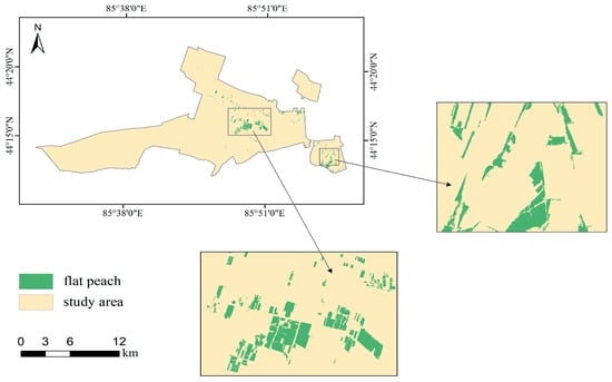
Figure 7.
Map of flat peaches in the study area in 2021.
4. Discussion
4.1. Effect Analysis of Features on Results
In remote sensing image classification, the selection and optimization of feature variables directly affect classification accuracy and efficiency [35,55]. Feature variable importance analysis showed that vegetation indices contribute significantly to the classification model. This conclusion was fully validated in the classification results of various schemes: Scheme 2, mainly composed of vegetation indices, achieved overall classification accuracies of over 90% in both pixel-based and object-based methods (Table 4). Scheme 3 added seven texture features to Scheme 2, but the overall classification accuracies based on pixel and object-based methods only increased by 0.2% and 2.05%, respectively. Many previous studies have also shown that spectral information plays a decisive role in land cover classification. Song et al. [16] found that the performance of classifiers mainly depends on spectral variables from multiple seasons, and the addition of texture variables only improves accuracy by 1%. For ground objects with similar spectral information, texture features can be effectively used for differentiation [17,56]. In this study, during the overwintering period, the flat peaches and grapes covered with plastic films had similar spectral information. In the object-based classification, compared with Scheme 1, Scheme 3 increased the PA of flat peaches and grapes by 20% and 19.51%, respectively, after adding GLCM variance, mean, and correlation (Table S1). Although adding texture features can reduce the difficulty of classifying ground objects with similar spectral information, it is unlikely to eliminate the impact of similar spectral information, which is consistent with the findings of Mueller et al. [57]. When the number of input feature variables exceeded 25, classification accuracy gradually decreased with the addition of other GLCM statistics. This indicated that too many input feature variables can cause data redundancy and reduce model performance. Shi et al. [58] also showed that feature optimization can reduce the participation of irrelevant feature variables while ensuring classification accuracy.
4.2. Effect Analysis of Classification Method on Results
The choice of classification method is crucial for improving classification accuracy [59]. In this study, the object-based classification outperformed the pixel-based classification. Except for Scheme 1, object-based classification improved the overall accuracy compared to pixel-based classification, which was consistent with the findings of Wu et al. [60] and Du et al. [61]. McNemar’s test showed that, except for scheme 2, the difference between pixel-based and object-based classification accuracy was significant at the 5% level. The findings in this study filled the comparison of object-based and pixel-based classifications on GF-1/PMS data. Lantz et al. [62] also reported that object-based methods significantly improved classification accuracy for wetland mapping using WorldView-2 imagery. However, when classifying agricultural landscapes using SPOT-5 HR images, it was found that utilizing the same machine learning algorithm, the difference between pixel-based and object-based classification accuracy was not statistically significant [40]. This indicates that the object-based method, using homogeneous image objects after segmentation as the basic classification unit, significantly reduces the spectral heterogeneity within classes [63,64], and thereby makes it more suitable for high-resolution remote sensing monitoring [38].
4.3. Error Analysis
The overlap between flat peaches, grapes, construction lands, and forests was not completely resolved in any of the classification approaches (Figure 5 and Figure 6). There was a heavy overlap between grapes and flat peaches, but the confusion matrix (Table S2) failed to reflect the fact. This is attributed to the number of grape validation samples is relatively small (Table 2), leading to an underestimation of the confusion between flat peaches and grapes. Therefore, in future research, it is necessary to ensure the adequacy of each category of samples. To further verify whether the confusion between flat peaches and grapes was caused by sample imbalance, we trained the pixel-based classification scheme 3 model using a class-balanced random forest algorithm, with the weights set as the inverse of the number of samples in each category. The results showed that the PA, F1 score, and IoU of grapes have significantly improved, while those of flat peaches have slightly decreased (Table S4). This may be attributed to the model’s increased effort to identify grapes, leading to a slight loss in precision for the majority class (flat peaches). We further conducted a local comparison of the mapping results produced by the two algorithms and found that the class-balanced random forest algorithm did not significantly improve the actual confusion between flat peaches and grapes (Figure S4a–c). Moreover, other land cover types in some local areas were misidentified as grapes (Figure S4d–f), leading to a decrease in overall mapping accuracy. This is attributed to the class-balanced model is more sensitive to grape recognition, and it mixes other land classes to find more grapes. This trade-off demonstrates that the primary reason for the confusion between grapes and flat peaches is the spectral similarity caused by the film covering [29], rather than sample imbalance.
We plotted the average spectral curves of flat peaches, grapes, construction lands, and forests (Figure 8). In pixel-based classification, the confusion between construction lands and flat peaches may stem from their relatively similar reflectance curves. The reflectance of grapes is slightly higher than that of forests, which has led to some grapes being misclassified as forests in object-based classification. Moreover, the shadows of the trees also caused some street trees and nearby flat peaches to be merged into a single object during the image segmentation process. To address the above confusion, future research could follow two strategies. Frist, the physical structure information from radar remote sensing data can serve as an important supplement to spectral information, alleviating the issue of low spectral separability [65,66,67]. Secondly, more spatial features can be combined to improve mapping accuracy [68]. The uncertainty of statistical data also affects the mapping accuracy of flat peaches. The statistical data was released by the Xinjiang Production and Construction Corps, and the results were derived from the aggregation of administrative district reports, which may result in either an underestimation or an overestimation of the flat peach planting area. However, the officially released statistical data remained a crucial foundation for assessing the accuracy of classification results, with its potential error falling within an acceptable range [6,69].
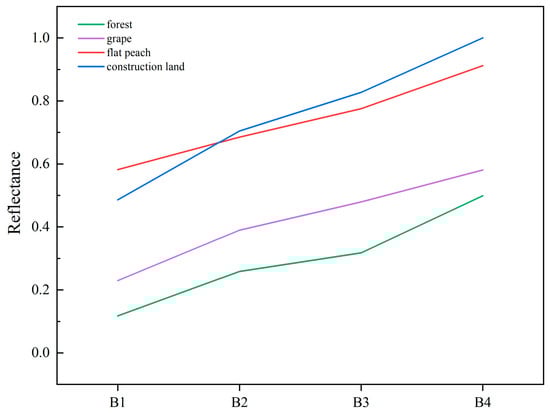
Figure 8.
The average spectral curves of flat peaches, grapes, construction lands, and forests.
4.4. Advantages and Applicability
This study confirms the feasibility of mapping flat peaches based on GF-1/PMS imagery during the overwintering period. To the best of our knowledge, our study is the first attempt to map fruit trees in temperate regions using phenological characteristics during the overwintering period. The use of phenological information from single-phase GF-1 images can allow us the opportunity to map flat peach distribution without requiring multi-temporal images. This significantly reduces the cost of acquiring high-resolution imagery and provides an economical and efficient method for mapping flat peaches in northern Xinjiang. Our method based on the overwintering window can be applied to mapping fruit trees that use similar agricultural protection measures. For example, vineyards in Italy covered with plastic film [70]. Orchards used other protective measures for overwintering can be mapped by the corresponding surface structural characteristics. For example, pomegranates in southern Xinjiang use the soil-burying method to overwinter [71], it is possible to map pomegranates based on the special shapes and textures of the soil ridges in the future. However, the methods used in this study may not be suitable for application to subtropical and tropical regions, where extremely low temperatures are not a concern and many fruit trees continue to grow during the winter [72].
Our study selected images after the snow and ice have melted, facing the issue that qualified images may be missing in a certain year. Sentinel-1 data can penetrate snow and ice cover [73,74], and its revisit period is 5 days, which provides effective support for the promotion of fruit tree mapping based on the overwintering window. The popularity of UAV platforms has also increased the feasibility of real-time forest monitoring at local scales [75]. In addition, to verify the interannual transferability of the object-based classification model [76], the classification Scheme 3 model constructed using 2021 GF-1 data was directly applied to the 2020 Sentinel-2 data. Specifically, we selected Sentinel-2 image from the same period (27 March) and used the distance metric method to transfer the 2021 training and validation samples to 2020. The number of samples for each category in 2020 is shown in Table S5. The results indicate that the model’s overall performance in 2020 was relatively acceptable, with an overall classification accuracy of 76.03%. It is predictable to obtain such a result. Because there is a significant difference in spatial resolution between GF-1 data (2 m) and Sentinel-2 data (10 m), pure pixels in GF-1 images may become mixed pixels in Sentinel-2 images. This alters the spectral characteristics of objects, causing the rules of models trained on high-resolution data to become partially ineffective when applied to medium-resolution data. Moreover, the limitations of supervised classification model restrict its applications [77], mainly manifested in their high dependence on training samples and weak generalization ability. It is also necessary to conduct further research in other regions with similar agricultural systems to verify the spatial robustness of this method in different areas [6]. Therefore, in future research, multi-source image data can be integrated through histogram matching, the sample size can be increased, and more optimized algorithms can be used to improve the comprehensiveness and accuracy of mapping.
5. Conclusions
The 2 m spatial resolution and 4-day revisit cycle of GF-1/PMS data provide a unique opportunity to map flat peaches based on the key overwintering window in this study. To the best of our knowledge, this study is the first to use a pixel-based and object-based random forest algorithm combined with agricultural film features for fruit tree mapping. The statistical differences between object-based classification and pixel-based classification are significant. Spectral information played a decisive role in classification, while texture features such as Var, Mean, and Cor also had a remarkable impact on improving accuracy. The high precision of flat peach mapping demonstrated the reliability of our method. The flat peach mapping method based on overwintering windows developed in this study has the potential to be applied to other similar agricultural management systems. However, additional case studies and method improvements are still required for further expansion of this method to other fruit trees and regions, especially orchards that do not use plastic film protection during overwintering. Future work should integrate multi-source remote sensing data and surface structure features to identify orchard mapping under other winter protection measures.
Supplementary Materials
The following supporting information can be downloaded at: https://www.mdpi.com/article/10.3390/f16101566/s1, Figure S1: Spatial distribution of training and validation samples; Figure S2: The optimal segmentation scale line by estimation of scale parameter (ESP); Figure S3: Results at different segmentation scales; Figure S4: Comparison of random forest algorithms; Table S1: Summary of changed sample points identified by the cosine-similarity check; Table S2: The accuracy confusion matrix is based on pixel and object-based classification methods; Table S3: Importance of the 25 input variables in Scheme 3; Table S4: Classification accuracy of grapes and flat peaches produced by pixel-based Scheme 3 using standard random forest algorithm and class-balanced random forest algorithm; Table S5: Land Cover Types and Their Sample Size in 2020.
Author Contributions
Conceptualization, Y.W. and C.T.; methodology, Y.W.; software, Y.W.; formal analysis, Y.W. and J.W.; investigation, Y.W. and C.T.; data curation, Y.W.; writing—original draft preparation, Y.W.; writing—review and editing, J.W. and C.T.; project administration, C.T.; funding acquisition, C.T. All authors have read and agreed to the published version of the manuscript.
Funding
This study was funded by the Key Areas Science and Technology Research Program (2021AB015) and the Research on Improving Quality and Efficiency of ‘Xin Feng Yuan’ Enzyme Fertilizer in Flat Peach and Grape Cultivation (20250158).
Data Availability Statement
The data presented in this study is available on request from the corresponding author.
Acknowledgments
The authors are grateful for the valuable comments from anonymous reviewers.
Conflicts of Interest
The authors declare no conflicts of interest.
References
- Tian, H.L.; Wang, P.; Zhan, P.; Yan, H.Y.; Zhou, W.J.; Zhang, F. Effects of β-glucosidase on the aroma characteristics of flat peach juice as assessed by descriptive sensory analysis and gas chromatography and compared by partial least squares regression. LWT Food Sci. Technol. 2017, 82, 113–120. [Google Scholar] [CrossRef]
- Faust, M.; Timon, B. Origin and Dissemination of Peach. In Horticultural Reviews; John Wiley & Sons, Inc.: Hoboken, NJ, USA, 1995; Volume 17. [Google Scholar]
- Temnani, A.; Berríos, P.; Zapata-García, S.; Pérez-Pastor, A. Deficit irrigation strategies of flat peach trees under semi-arid conditions. Agric. Water Manag. 2023, 287, 108464. [Google Scholar] [CrossRef]
- Nicotra, A.; Conte, L.; Moser, L.; Fantechi, P. New types of high quality peaches: Flat peaches (P. persica var. platicarpa) and Ghiaccio peach series with long on tree fruit life. In Proceedings of the 5th International Peach Symposium, Davis, CA, USA, 8–11 July 2001; pp. 131–135. [Google Scholar]
- Huan, L.; Yao, Z.; Chong, W.; Yanfei, S.; Yonghui, L. Community structure analysis of yeast attached to flat peach leaves in Xinjiang. Ecol. Sci. 2019, 38, 29–34. [Google Scholar] [CrossRef]
- Xun, L.; Zhang, J.; Cao, D.; Wang, J.; Zhang, S.; Yao, F. Mapping cotton cultivated area combining remote sensing with a fused representation-based classification algorithm. Comput. Electron. Agric. 2021, 181, 105940. [Google Scholar] [CrossRef]
- Luan, W.J.; Shen, X.J.; Fu, Y.H.; Li, W.C.; Liu, Q.L.; Wang, T.; Ma, D.X. Research on Maize Acreage Extraction and Growth Monitoring Based on a Machine Learning Algorithm and Multi-Source Remote Sensing Data. Sustainability 2023, 15, 16343. [Google Scholar] [CrossRef]
- da Silva, C.A.; Leonel, A.H.S.; Rossi, F.S.; Correia, W.L.F.; Santiago, D.D.; de Oliveira, J.F.; Teodoro, P.E.; Lima, M.; Capristo-Silva, G.F. Mapping soybean planting area in midwest Brazil with remotely sensed images and phenology-based algorithm using the Google Earth Engine platform. Comput. Electron. Agric. 2020, 169, 105194. [Google Scholar] [CrossRef]
- Zhong, K.W.; Zuo, J.; Xu, J.H. Rice Identification and Spatio-Temporal Changes Based on Sentinel-1 Time Series in Leizhou City, Guangdong Province, China. Remote Sens. 2025, 17, 39. [Google Scholar] [CrossRef]
- Minh, H.V.T.; Avtar, R.; Mohan, G.; Misra, P.; Kurasaki, M. Monitoring and Mapping of Rice Cropping Pattern in Flooding Area in the Vietnamese Mekong Delta Using Sentinel-1A Data: A Case of An Giang Province. ISPRS Int. J. Geo-Inf. 2019, 8, 211. [Google Scholar] [CrossRef]
- Qin, Y.W.; Xiao, X.M.; Dong, J.W.; Zhou, Y.T.; Zhu, Z.; Zhang, G.L.; Du, G.M.; Jin, C.; Kou, W.L.; Wang, J.; et al. Mapping paddy rice planting area in cold temperate climate region through analysis of time series Landsat 8 (OLI), Landsat 7 (ETM+) and MODIS imagery. ISPRS J. Photogramm. Remote Sens. 2015, 105, 220–233. [Google Scholar] [CrossRef]
- Dong, J.W.; Xiao, X.M.; Kou, W.L.; Qin, Y.W.; Zhang, G.L.; Li, L.; Jin, C.; Zhou, Y.T.; Wang, J.; Biradar, C.; et al. Tracking the dynamics of paddy rice planting area in 1986-2010 through time series Landsat images and phenology-based algorithms. Remote Sens. Environ. 2015, 160, 99–113. [Google Scholar] [CrossRef]
- Zhang, W.M.; Brandt, M.; Prishchepov, A.V.; Li, Z.F.; Lyu, C.G.; Fensholt, R. Mapping the Dynamics of Winter Wheat in the North China Plain from Dense Landsat Time Series (1999 to 2019). Remote Sens. 2021, 13, 1170. [Google Scholar] [CrossRef]
- le Maire, G.; Dupuy, S.; Nouvellon, Y.; Loos, R.A.; Hakarnada, R. Mapping short-rotation plantations at regional scale using MODIS time series: Case of eucalypt plantations in Brazil. Remote Sens. Environ. 2014, 152, 136–149. [Google Scholar] [CrossRef]
- Zhang, G.L.; Xiao, X.M.; Dong, J.W.; Kou, W.L.; Jin, C.; Qin, Y.W.; Zhou, Y.T.; Wang, J.; Menarguez, M.A.; Biradar, C. Mapping paddy rice planting areas through time series analysis of MODIS land surface temperature and vegetation index data. ISPRS J. Photogramm. Remote Sens. 2015, 106, 157–171. [Google Scholar] [CrossRef]
- Song, Q.; Zhou, Q.B.; Wu, W.B.; Hu, Q.; Lu, M.; Liu, S.B. Mapping regional cropping patterns by using GF-1 WFV sensor data. J. Integr. Agric. 2017, 16, 337–347. [Google Scholar] [CrossRef]
- Luo, H.X.; Dai, S.P.; Li, M.F.; Liu, E.P.; Zheng, Q.; Hu, Y.Y.; Yi, X.P. Comparison of machine learning algorithms for mapping mango plantations based on Gaofen-1 imagery. J. Integr. Agric. 2020, 19, 2815–2828. [Google Scholar] [CrossRef]
- Cai, Y.P.; Guan, K.Y.; Peng, J.; Wang, S.W.; Seifert, C.; Wardlow, B.; Li, Z. A high-performance and in-season classification system of field-level crop types using time-series Landsat data and a machine learning approach. Remote Sens. Environ. 2018, 210, 35–47. [Google Scholar] [CrossRef]
- Qi, N.; Yang, H.; Shao, G.W.; Chen, R.Q.; Wu, B.G.; Xu, B.; Feng, H.K.; Yang, G.J.; Zhao, C.J. Mapping tea plantations using multitemporal spectral features by harmonised Sentinel-2 and Landsat images in Yingde, China. Comput. Electron. Agric. 2023, 212, 108108. [Google Scholar] [CrossRef]
- Yin, Q.; Liu, M.L.; Cheng, J.Y.; Ke, Y.H.; Chen, X.W. Mapping Paddy Rice Planting Area in Northeastern China Using Spatiotemporal Data Fusion and Phenology-Based Method. Remote Sens. 2019, 11, 1699. [Google Scholar] [CrossRef]
- Bargiel, D. A new method for crop classification combining time series of radar images and crop phenology information. Remote Sens. Environ. 2017, 198, 369–383. [Google Scholar] [CrossRef]
- Zhou, Y.N.; Luo, J.C.; Feng, L.; Yang, Y.P.; Chen, Y.H.; Wu, W. Long-short-term-memory-based crop classification using high-resolution optical images and multi-temporal SAR data. GISci. Remote Sens. 2019, 56, 1170–1191. [Google Scholar] [CrossRef]
- Xu, J.X.; Chen, C.; Zhou, S.T.; Hu, W.M.; Zhang, W. Land use classification in mine-agriculture compound area based on multi-feature random forest: A case study of Peixian. Front. Sustain. Food Syst. 2024, 7, 1335292. [Google Scholar] [CrossRef]
- Wei, D.S.; Hou, D.Y.; Zhou, X.G.; Chen, J. Change Detection Using a Texture Feature Space Outlier Index from Mono-Temporal Remote Sensing Images and Vector Data. Remote Sens. 2021, 13, 3857. [Google Scholar] [CrossRef]
- Zhao, Z.; Dong, J.; Zhang, G.; Yang, J.; Liu, R.; Wu, B.; Xiao, X. Improved phenology-based rice mapping algorithm by integrating optical and radar data. Remote Sens. Environ. 2024, 315, 114460. [Google Scholar] [CrossRef]
- Li, M.; Zhao, G.-X.; Qin, Y.-W. Extraction and Monitoring of Cotton Area and Growth Information Using Remote Sensing at Small Scale: A Case Study in Dingzhuang Town of Guangrao County, China. In Proceedings of the 2011 International Conference on Computer Distributed Control and Intelligent Environmental Monitoring, Changsha, China, 19–20 February 2011; pp. 816–823. [Google Scholar]
- Ashourloo, D.; Shahrabi, H.S.; Azadbakht, M.; Aghighi, H.; Nematollahi, H.; Alimohammadi, A.; Matkan, A.A. Automatic canola mapping using time series of sentinel 2 images. ISPRS J. Photogramm. Remote Sens. 2019, 156, 63–76. [Google Scholar] [CrossRef]
- Pu, Y.J. Analysis of Climate Characteristics of High-Quality Flat Peaches in Northern Xinjiang. Shihezi Sci. Technol. 2018, 5–7. [Google Scholar]
- Di, Y.; Dong, J.; Zhu, F.; Fu, P. A robust but straightforward phenology-based ginger mapping algorithm by using unique phenology features, and time-series Sentinel-2 images. Comput. Electron. Agric. 2022, 198, 107066. [Google Scholar] [CrossRef]
- Ghosh, A.; Joshi, P.K. A comparison of selected classification algorithms for mapping bamboo patches in lower Gangetic plains using very high resolution WorldView 2 imagery. Int. J. Appl. Earth Obs. Geoinf. 2014, 26, 298–311. [Google Scholar] [CrossRef]
- Chuang, Y.-C.; Shiu, Y.-S. A Comparative Analysis of Machine Learning with WorldView-2 Pan-Sharpened Imagery for Tea Crop Mapping. Sensors 2016, 16, 594. [Google Scholar] [CrossRef] [PubMed]
- Tuxen, K.; Schile, L.; Stralberg, D.; Siegel, S.; Parker, T.; Vasey, M.; Callaway, J.; Kelly, M. Mapping changes in tidal wetland vegetation composition and pattern across a salinity gradient using high spatial resolution imagery. Wetl. Ecol. Manag. 2010, 19, 141–157. [Google Scholar] [CrossRef]
- Li, M.; Ma, L.; Blaschke, T.; Cheng, L.; Tiede, D. A systematic comparison of different object-based classification techniques using high spatial resolution imagery in agricultural environments. Int. J. Appl. Earth Obs. Geoinf. 2016, 49, 87–98. [Google Scholar] [CrossRef]
- Szantoi, Z.; Escobedo, F.J.; Abd-Elrahman, A.; Pearlstine, L.; Dewitt, B.; Smith, S. Classifying spatially heterogeneous wetland communities using machine learning algorithms and spectral and textural features. Environ. Monit. Assess. 2015, 187, 262. [Google Scholar] [CrossRef]
- Yang, Z.Q.; Dong, J.W.; Kou, W.L.; Qin, Y.W.; Xiao, X.M. Mapping Panax Notoginseng Plantations by Using an Integrated Pixel- and Object-Based (IPOB) Approach and ZY-3 Imagery. Remote Sens. 2021, 13, 2184. [Google Scholar] [CrossRef]
- Pelletier, C.; Valero, S.; Inglada, J.; Champion, N.; Dedieu, G. Assessing the robustness of Random Forests to map land cover with high resolution satellite image time series over large areas. Remote Sens. Environ. 2016, 187, 156–168. [Google Scholar] [CrossRef]
- Fu, B.; Xie, S.; He, H.; Zuo, P.; Sun, J.; Liu, L.; Huang, L.; Fan, D.; Gao, E. Synergy of multi-temporal polarimetric SAR and optical image satellite for mapping of marsh vegetation using object-based random forest algorithm. Ecol. Indic. 2021, 131, 108173. [Google Scholar] [CrossRef]
- Fu, B.L.; Wang, Y.Q.; Campbell, A.; Li, Y.; Zhang, B.; Yin, S.B.; Xing, Z.F.; Jin, X.M. Comparison of object-based and pixel-based Random Forest algorithm for wetland vegetation mapping using high spatial resolution GF-1 and SAR data. Ecol. Indic. 2017, 73, 105–117. [Google Scholar] [CrossRef]
- Wang, D.; Wan, B.; Qiu, P.; Su, Y.; Guo, Q.; Wu, X. Artificial Mangrove Species Mapping Using Pléiades-1: An Evaluation of Pixel-Based and Object-Based Classifications with Selected Machine Learning Algorithms. Remote Sens. 2018, 10, 294. [Google Scholar] [CrossRef]
- Duro, D.C.; Franklin, S.E.; Dubé, M.G. A comparison of pixel-based and object-based image analysis with selected machine learning algorithms for the classification of agricultural landscapes using SPOT-5 HRG imagery. Remote Sens. Environ. 2012, 118, 259–272. [Google Scholar] [CrossRef]
- Huang, H.; Wang, J.; Liu, C.; Liang, L.; Li, C.; Gong, P. The migration of training samples towards dynamic global land cover mapping. ISPRS J. Photogramm. Remote Sens. 2020, 161, 27–36. [Google Scholar] [CrossRef]
- Witharana, C.; Civco, D.L.; Meyer, T.H. Evaluation of data fusion and image segmentation in earth observation based rapid mapping workflows. ISPRS J. Photogramm. Remote Sens. 2014, 87, 1–18. [Google Scholar] [CrossRef]
- Drǎguţ, L.; Tiede, D.; Levick, S.R. ESP: A tool to estimate scale parameter for multiresolution image segmentation of remotely sensed data. Int. J. Geogr. Inf. Sci. 2010, 24, 859–871. [Google Scholar] [CrossRef]
- Rodríguez-Esparragón, D.; Marcello, J.; Eugenio, F.; Gamba, P. Index-based forest degradation mapping using high and medium resolution multispectral sensors. Int. J. Digit. Earth 2024, 17, 2365981. [Google Scholar] [CrossRef]
- Mohammadpour, P.; Viegas, D.X.; Viegas, C. Vegetation Mapping with Random Forest Using Sentinel 2 and GLCM Texture Feature—A Case Study for Lousã Region, Portugal. Remote Sens. 2022, 14, 4585. [Google Scholar] [CrossRef]
- Wan, L.; Li, Y.; Cen, H.; Zhu, J.; Yin, W.; Wu, W.; Zhu, H.; Sun, D.; Zhou, W.; He, Y. Combining UAV-Based Vegetation Indices and Image Classification to Estimate Flower Number in Oilseed Rape. Remote Sens. 2018, 10, 1484. [Google Scholar] [CrossRef]
- Breiman, L. Random forests. Mach. Learn. 2001, 45, 5–32. [Google Scholar] [CrossRef]
- Rudiyanto; Minasny, B.; Shah, R.M.; Soh, N.C.; Arif, C.; Setiawan, B.I. Automated Near-Real-Time Mapping and Monitoring of Rice Extent, Cropping Patterns, and Growth Stages in Southeast Asia Using Sentinel-1 Time Series on a Google Earth Engine Platform. Remote Sens. 2019, 11, 1666. [Google Scholar] [CrossRef]
- Jin, Y.H.; Liu, X.P.; Chen, Y.M.; Liang, X. Land-cover mapping using Random Forest classification and incorporating NDVI time-series and texture: A case study of central Shandong. Int. J. Remote Sens. 2018, 39, 8703–8723. [Google Scholar] [CrossRef]
- Fan, J.L.; Defourny, P.; Zhang, X.Y.; Dong, Q.H.; Wang, L.M.; Qin, Z.H.; De Vroey, M.; Zhao, C.L. Crop Mapping with Combined Use of European and Chinese Satellite Data. Remote Sens. 2021, 13, 4641. [Google Scholar] [CrossRef]
- De Vroey, M.; de Vendictis, L.; Zavagli, M.; Bontemps, S.; Heymans, D.; Radoux, J.; Koetz, B.; Defourny, P. Mowing detection using Sentinel-1 and Sentinel-2 time series for large scale grassland monitoring. Remote Sens. Environ. 2022, 280, 113145. [Google Scholar] [CrossRef]
- Zhang, Q.; Wang, G.; Wang, G.; Song, W.; Wei, X.; Hu, Y. Identifying Winter Wheat Using Landsat Data Based on Deep Learning Algorithms in the North China Plain. Remote Sens. 2023, 15, 5121. [Google Scholar] [CrossRef]
- Foody, G.M. Thematic map comparison: Evaluating the Statistical significance of differences in classification accuracy. Photogramm. Eng. Remote Sens. 2004, 70, 627–633. [Google Scholar] [CrossRef]
- Shahrokh, V.; Khademi, H.; Zeraatpisheh, M. Mapping clay mineral types using easily accessible data and machine learning techniques in a scarce data region: A case study in a semi-arid area in Iran. Catena 2023, 223, 106932. [Google Scholar] [CrossRef]
- Xiao, T.; She, B.; Zhao, J.L.; Huang, L.S.; Ruan, C.; Huang, W.J. Identification of soybean planting areas using Sentinel-1/2 remote sensing data: A combined approach of reduced redundancy feature optimization and ensemble learning. Eur. J. Agron. 2025, 164, 127480. [Google Scholar] [CrossRef]
- Peña-Barragán, J.M.; Ngugi, M.K.; Plant, R.E.; Six, J. Object-based crop identification using multiple vegetation indices, textural features and crop phenology. Remote Sens. Environ. 2011, 115, 1301–1316. [Google Scholar] [CrossRef]
- Mueller, M.; Segl, K.; Kaufmann, H. Edge- and region-based segmentation technique for the extraction of large, man-made objects in high-resolution satellite imagery. Pattern Recognit. 2004, 37, 1619–1628. [Google Scholar] [CrossRef]
- Shi, Y.F.; Zhang, P.H.; Wang, Z.Y. Extraction of Lilium davidii var. unicolor Planting Information Based on Deep Learning and Multi-Source Data. Sensors 2024, 24, 1543. [Google Scholar] [CrossRef]
- Li, C.C.; Wang, J.; Wang, L.; Hu, L.Y.; Gong, P. Comparison of Classification Algorithms and Training Sample Sizes in Urban Land Classification with Landsat Thematic Mapper Imagery. Remote Sens. 2014, 6, 964–983. [Google Scholar] [CrossRef]
- Wu, N.T.; Crusiol, L.G.T.; Liu, G.X.; Wuyun, D.; Han, G.D. Comparing Machine Learning Algorithms for Pixel/Object-Based Classifications of Semi-Arid Grassland in Northern China Using Multisource Medium Resolution Imageries. Remote Sens. 2023, 15, 750. [Google Scholar] [CrossRef]
- Du, B.J.; Mao, D.H.; Wang, Z.M.; Qiu, Z.Q.; Yan, H.Q.; Feng, K.D.; Zhang, Z.B. Mapping Wetland Plant Communities Using Unmanned Aerial Vehicle Hyperspectral Imagery by Comparing Object/Pixel-Based Classifications Combining Multiple Machine-Learning Algorithms. IEEE J. Sel. Top. Appl. Earth Obs. Remote Sens. 2021, 14, 8249–8258. [Google Scholar] [CrossRef]
- Lantz, N.J.; Wang, J. Object-based classification of Worldview-2 imagery for mapping invasive common reed, Phragmites australis. Can. J. Remote Sens. 2014, 39, 328–340. [Google Scholar] [CrossRef]
- Blaschke, T. Object based image analysis for remote sensing. ISPRS J. Photogramm. Remote Sens. 2010, 65, 2–16. [Google Scholar] [CrossRef]
- Kaszta, Z.; Van de Kerchove, R.; Ramoelo, A.; Cho, M.A.; Madonsela, S.; Mathieu, R.; Wolff, E. Seasonal Separation of African Savanna Components Using Worldview-2 Imagery: A Comparison of Pixel- and Object-Based Approaches and Selected Classification Algorithms. Remote Sens. 2016, 8, 763. [Google Scholar] [CrossRef]
- Wang, J.; Xiao, X.; Qin, Y.; Dong, J.; Geissler, G.; Zhang, G.; Cejda, N.; Alikhani, B.; Doughty, R.B. Mapping the dynamics of eastern redcedar encroachment into grasslands during 1984–2010 through PALSAR and time series Landsat images. Remote Sens. Environ. 2017, 190, 233–246. [Google Scholar] [CrossRef]
- Cheng, Y.; Yu, L.; Cracknell, A.P.; Gong, P. Oil palm mapping using Landsat and PALSAR: A case study in Malaysia. Int. J. Remote Sens. 2016, 37, 5431–5442. [Google Scholar] [CrossRef]
- Collins, L.; Guindon, L.; Lloyd, C.; Taylor, S.W.; White, S. Fractional cover mapping of wildland-urban interface fuels using Landsat, Sentinel 1 and PALSAR imagery. Remote Sens. Environ. 2024, 308, 114189. [Google Scholar] [CrossRef]
- Tiwari, A.; Silver, M.; Karnieli, A. Developing object-based image procedures for classifying and characterising different protected agriculture structures using LiDAR and orthophoto. Biosyst. Eng. 2020, 198, 91–104. [Google Scholar] [CrossRef]
- Miao, C.; Fu, S.; Sun, W.; Feng, S.; Hu, Y.; Liu, J.; Feng, Q.; Li, Y.; Liang, T. Large-scale mapping of the spatial distribution and cutting intensity of cultivated alfalfa based on a sample generation algorithm and random forest. Comput. Electron. Agric. 2025, 237, 110613. [Google Scholar] [CrossRef]
- Farbo, A.; Trombetta, N.G.; de Palma, L.; Borgogno-Mondino, E. Estimation of Intercepted Solar Radiation and Stem Water Potential in a Table Grape Vineyard Covered by Plastic Film Using Sentinel-2 Data: A Comparison of OLS-, MLR-, and ML-Based Methods. Plants 2024, 13, 1203. [Google Scholar] [CrossRef]
- Huang, M.Z.; Guan, S.H.; Chai, Y.Q.; Xu, J.; Yang, Y.L.; Liu, H.Y.; Yang, L.; Diao, M. Study on the protective effect of cold-proof and wintering measures on Tunisia soft-seed pomegranate. J. Fruit Sci. 2024, 41, 929–940. [Google Scholar] [CrossRef]
- Raju, C.; Pazhanivelan, S.; Perianadar, I.V.; Kaliaperumal, R.; Sathyamoorthy, N.K.; Sendhilvel, V. Climate Change as an Existential Threat to Tropical Fruit Crop Production—A Review. Agriculture 2024, 14, 2018. [Google Scholar] [CrossRef]
- Bulovic, N.; Johnson, F.; Lievens, H.; Shaw, T.E.; McPhee, J.; Gascoin, S.; Demuzere, M.; McIntyre, N. Evaluating the Performance of Sentinel-1 SAR Derived Snow Depth Retrievals Over the Extratropical Andes Cordillera. Water Resour. Res. 2025, 61, e2024WR037766. [Google Scholar] [CrossRef]
- Feng, T.; Huang, C.; Huang, G.; Shao, D.; Hao, X. Estimating snow depth based on dual polarimetric radar index from Sentinel-1 GRD data: A case study in the Scandinavian Mountains. Int. J. Appl. Earth Obs. Geoinf. 2024, 130, 103873. [Google Scholar] [CrossRef]
- Pham, V.T.; Do, T.A.T.; Tran, H.D.; Do, A.N.T. Classifying forest cover and mapping forest fire susceptibility in Dak Nong province, Vietnam utilizing remote sensing and machine learning. Ecol. Inform. 2024, 79, 102392. [Google Scholar] [CrossRef]
- Zhao, H.; Zhou, Y.; Zhang, G.; Chen, X.; Chang, Y.; Luo, Y.; Jin, Y.; Pan, Z.; An, P. Mapping the dynamics of intensive forage acreage during 2008–2022 in Google Earth Engine using time series Landsat images and a phenology-based algorithm. Comput. Electron. Agric. 2024, 221, 108983. [Google Scholar] [CrossRef]
- Sen, P.C.; Hajra, M.; Ghosh, M. Supervised Classification Algorithms in Machine Learning: A Survey and Review. In Emerging Technology in Modelling and Graphics; Advances in Intelligent Systems and Computing; Springer: Singapore, 2020; pp. 99–111. [Google Scholar]
Disclaimer/Publisher’s Note: The statements, opinions and data contained in all publications are solely those of the individual author(s) and contributor(s) and not of MDPI and/or the editor(s). MDPI and/or the editor(s) disclaim responsibility for any injury to people or property resulting from any ideas, methods, instructions or products referred to in the content. |
© 2025 by the authors. Licensee MDPI, Basel, Switzerland. This article is an open access article distributed under the terms and conditions of the Creative Commons Attribution (CC BY) license (https://creativecommons.org/licenses/by/4.0/).