Article

Spatial Distribution and Intraspecific and Interspecific Association in a Deciduous Broad-Leaved Forest in East China

Jiangxi Provincial Key Laboratory of Carbon Neutrality and Ecosystem Carbon Sink, Lushan Botanical Garden, Jiangxi Province and Chinese Academy of Sciences, Jiujiang 332900, China
*
Author to whom correspondence should be addressed.
Forests 2025, 16(10), 1511; https://doi.org/10.3390/f16101511
Submission received: 23 July 2025 / Revised: 12 September 2025 / Accepted: 21 September 2025 / Published: 24 September 2025
(This article belongs to the Special Issue Modeling of Forest Dynamics and Species Distribution)

Abstract

The spatial distribution of plant species is a crucial indicator of the mechanisms driving competition or coexistence both within and between populations and communities. Analyzing these patterns provides essential insights into fundamental ecological processes and aids in evaluating ecological hypotheses. To study the spatial distribution of dominant tree species and their associations both within and among species, we established a 25-hectare forest plot in Lushan Mountain. We employed the g(r) function alongside three null models—complete spatial randomness (CSR), heterogeneous Poisson (HP), and antecedent condition (AC)—to analyze spatial patterns and assess species interactions at various life stages. Additionally, we examined the relationships between spatial distributions and environmental factors such as soil properties and topography using Berman’s test. Our results showed that all 12 dominant tree species exhibited significant aggregation under the CSR model; however, the scales of aggregation were reduced under the HP model. We also found evidence of aggregation among multiple species across different life stages and tree layers under CSR. Notably, this pattern persisted under the AC model but was limited to specific spatial scales. Furthermore, elevation, topographical convexity, and the total content of soil nitrogen (N) and carbon (C) were identified as statistically significant predictors of species distributions. Overall, these findings highlight that both biological and environmental factors play a vital role in shaping plant spatial patterns across different scales.

1. Introduction

Plant spatial distribution patterns refer to the arrangement of plant populations or communities in a specific area, which typically is not random. These patterns reflect the influence of both biotic and abiotic factors during ecological processes [1]. The spatial arrangement of plants can, in turn, affect the relationships within their species (intra-specific) and between different species (inter-specific), ultimately driving community dynamics [2,3]. Spatial patterns can be influenced by environmental variability, biological processes such as seed dispersal and clonal propagation, and local biotic interactions like competition and facilitation. For instance, competition may lead to segregated spatial patterns, while aggregated patterns can occur due to limited seed dispersal or the presence of habitat mosaics. Studying these patterns helps to reveal mechanisms of species coexistence, including inter-specific relationships and environmental influences, which are essential for understanding forest community succession and population maintenance [4]. However, the specific mechanisms that drive these spatial patterns remain unclear and require further research, particularly in subtropical forests [5,6].
Scale plays a critical role in spatial pattern research because plant distribution patterns may change as the spatial scale increases, with different factors influencing patterns across various scale ranges [7]. Additionally, plants at different life stages or within distinct layers can exhibit varying competitive abilities [8]. For example, canopy trees have a significant competitive advantage in acquiring light, which can hinder the survival of surrounding plants [9]. Topographic factors, such as elevation and slope, along with soil characteristics, can create unique habitats for certain plants, leading to aggregated patterns at fine scales but resulting in randomness at broader scales [10,11,12]. Dominant tree species are particularly valuable research subjects due to their broad ecological niches and effective survival strategies [13,14]. They make ideal candidates for studying intra-specific and inter-specific associations, as well as the impact of environmental factors on plant distribution.
Density-dependent effects—such as distance-dependent mortality and the abundance of offspring near their parents (as described by the Janzen-Connell hypothesis) [15], density-dependent thinning (known as the random-mortality hypothesis) [16], and community compensatory trends (CCT)—are among the most widely discussed hypotheses for explaining intra-species associations. The Unified Neutral Theory, the negative density-dependent hypothesis, and niche differentiation theory are the three primary theories that explain mechanisms of species coexistence [17]. However, experimental studies indicate that dispersal strategies significantly impact spatial structure, particularly at fine scales. Nonetheless, the direct relationship between spacer length and pattern formation requires further validation [18,19].
Numerous studies have examined the spatial patterns and assembly mechanisms of tropical forests [7]. However, relatively few have focused on species coexistence in deciduous forests, which differ fundamentally from evergreen forests because of their seasonal leaf-shedding nature. A fifty-year study of spatial patterns in deciduous forests suggested that a random distribution may represent a more natural state in semi-natural deciduous stands. Canopy gaps were identified as the primary drivers of spatial structural changes in these forests. Interestingly, competition seems to have a limited influence on adult tree mortality, while wind damage and other abiotic disturbances play a more significant role [20]. This underscores the distinct contributions of biotic and abiotic factors in shaping deciduous forest communities. Moreover, tropical deciduous plants possess a range of functional traits that enhance their adaptation to seasonal aridity. These traits include high specific leaf area (SLA), elevated photosynthetic rates, short leaf lifespans, and high wood density [21]. Evergreen and deciduous forests exhibit strategic differences in these functional traits: deciduous communities focus on rapid resource acquisition through high SLA and nutrient content to adapt to short growing seasons, whereas evergreen communities emphasize resource conservation and long-term survival via high carbon content and structural investment [22].
While previous studies have identified various mechanisms that allow species to coexist in temperate forests—such as light competition, habitat preferences, and regeneration strategies [13,19]—the specific processes driving spatial patterns remain unclear. This study examines a deciduous broad-leaved forest in Lushan Mountain, China, with the goal of analyzing the spatial distribution of dominant tree species and their relationships with environmental factors. The key scientific questions addressed are as follows: (1) What are the distribution patterns of dominant tree species, and are these patterns influenced by environmental heterogeneity or dispersal limitation? (2) What are the ecological implications of intra-specific and inter-specific associations at different scales? How do environmental factors influence species’ spatial distribution? This study integrates multiple ecological hypotheses to explain the spatial distribution patterns and coexistence mechanisms of dominant tree species in the deciduous broad-leaved forest of Lushan Mountain.

2. Materials and Methods

2.1. Study Site

A 25-hectare forest plot of subtropical deciduous broad-leaved forest was sampled in Lushan Mountain, located in the southeastern part of Jiujiang City, Jiangxi Province, China (Figure 1). The mountain borders the Yangtze River to the north and faces Poyang Lake to the east. It is positioned between 115°52′ and 116°8′ E longitude and 29°26′ and 29°41′ N latitude, within a subtropical monsoon climate zone characterized by mild and humid conditions. While the area’s natural zonal vegetation consists mainly of subtropical evergreen broad-leaved forests, large-scale afforestation campaigns since the 1930s have led to the development of extensive coniferous vegetation landscapes. The current vegetation reflects recovering secondary growth, exhibiting notable vertical distribution characteristics.

2.2. Data Collection

The 25-hectare forest monitoring plot near Yangtianping on Lushan Mountain extends in a northwest-southeast direction and measures 500 m in both length and width, with elevations ranging from 940 to 1174 m. This study established the Lushan Mountain Forest Dynamics Monitoring Plot between 2020 and 2021, following the technical protocols set by the Center for Tropical Forest Science (CTFS). A differential GPS system (Stonex S9 GPS System Gnss Rtk, China) was utilized to divide the 25-hectare plot into 625 quadrats, each measuring 20 m by 20 m, resulting in 25 quadrats per row and per column. All woody plants, with a minimum height of 1.3 m and a minimum diameter at breast height (DBH) of 1 cm, were inventoried. The recorded data included species name, DBH, coordinates, tree height, and environmental factors such as elevation, slope, aspect, and canopy coverage. The data regarding the dominant tree species and topographic factors in all 625 quadrats were collected in 2021.
Soil samples were collected from the center of each 20 m × 20 m quadrat and its four nested 10 m × 10 m sub-quadrats at a depth of 0–20 cm using a 5 cm diameter soil drill. The five samples from each point were combined to form one composite sample per quadrat for laboratory analysis. Additionally, an undisturbed soil core was extracted from the center of each quadrat using a 100 cm3 ring knife to measure soil bulk density. The soil properties were determined using standardized analytical procedures. Total carbon and total nitrogen were analyzed simultaneously using an elemental analyzer (Thermo Fisher Scientific, Braunschweig, Germany). Total phosphorus was measured by alkali fusion followed by molybdenum antimony spectrophotometry (UV-1800PC, Shanghai Mapada, Shanghai, China), while total potassium was determined by alkali fusion and flame photometry (FP6410, Shanghai Yidian Analysis, Shanghai, China). Soil pH was measured potentiometrically in a soil-water suspension (PB-10, Sartorius, Göttingen, Germany). Alkali hydrolyzable nitrogen was assessed using the alkali hydrolysis-diffusion method. Available phosphorus was extracted with ammonium fluoride-hydrochloric acid solution (for soils with pH < 6.5) and quantified by molybdenum antimony spectrophotometry. Finally, available potassium was extracted with ammonium acetate solution and measured by flame photometry [23]. A total of 625 soil samples, one from each quadrat, were collected and analyzed in 2023.

2.3. Data Analysis

We selected 12 dominant species based on their relative importance values index (relative IVI) ranks and categorized them into three life stage classes according to their layers and diameter at breast height (DBH). The relative IVI is calculated as follows: relative IVI = (relative dominance + relative abundance + relative frequency)/3. For tree layers, we defined the size categories as follows: 1–5 cm in DBH as small trees, 5–20 cm as medium trees, and 20 cm or greater as large individuals. For sub-arbor layers, the classifications are 1–5 cm as small trees, 5–10 cm as medium trees, and 10 cm or greater as large individuals. For shrub layers, we defined the categories as 1–1.5 cm as small shrubs, 1.5–2.5 cm as medium shrubs, and 2.5 cm or greater as large individuals [24].
Pair correlation function g(r) was chosen to implement spatial distribution analysis. g(r) function is a transformation of Ripley’s K-function K(r), which can effectively eliminate the cumulative effect [25]. The formula is as follows:
g r = K r 2 π r
g(r) = 1 indicates points of the pattern are random, g(r) > 1 indicates points of the pattern are aggregated, g(r) < 1 indicates points of the pattern are segregated. Complete spatial randomness (CSR) and heterogeneous Poisson (HP) were chosen as the null models in this function.
Pair correlation function g12(r) was chosen to achieve intra-specific and inter-specific space association analysis. The g12(r) function is from K12(r), which is a bivariate analysis of the K(r) function:
g 12 ( r ) = K 12 ( r ) 2 π r
CSR and the antecedent condition (AC) were selected as the null models [26,27]. The AC null model can assume that the positions of big individuals were constant, and the positions of smaller ones were randomized to reflect the space impact of big individuals to smaller ones. In total, 99 Monte Carlo simulations were conducted to obtain 98% confidence intervals to test the significance of departure from a null model [28].
Principal Component Analysis (PCA) was used to pick up key factors from 13 soil variables. Berman’s test was chosen to determine the association between the point patterns of dominant trees and spatial covariates (topographic and soil variables) [29]. This test compares the observed distribution of the values of a spatial covariate v(x), taken at the locations x of the points i of a point pattern, and the predicted distribution of the same covariate under CSR null model. Statistics ( Z 1 ) can be displayed as follows:
Z 1 = ( S μ ) / σ
S is the covariate values v(xi) at the points xi of the observed pattern. The μ value is the predicted value of S under CSR, and σ is the corresponding variance. Z 1 < 0, representing negative association between patterns and environment covariate, and if Z 1 > 0, the association is positive [23]. According to the statistic Z 1 and the p-value of Z 1 , we can test the association between point patterns and topographic and soil factors. Function g(r), g12(r) and Berman’s test were conducted using the “spatstat” package in R (version 4.5.0) [30,31].

3. Results

3.1. Taxonomic and Ecological Characteristics and Distribution Plot of Dominant Species

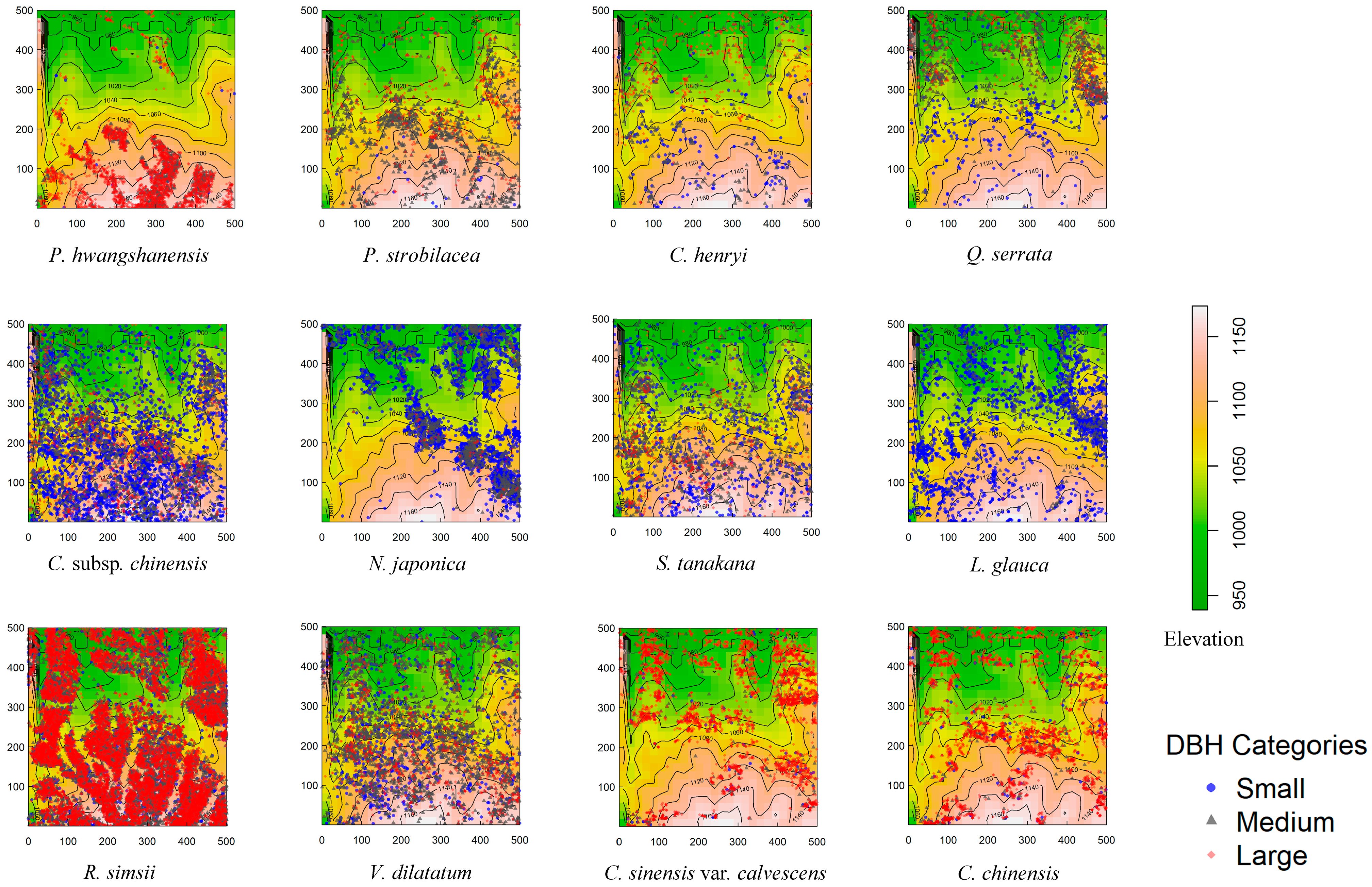
The twelve dominant species exhibit distinct taxonomic and ecological characteristics [32,33] (Table 1), varied life stage abundances (Table 2), and specific spatial distributions (Figure 2). Deciduous broad-leaved species dominate in terms of abundance and diameter at breast height (DBH), displaying clear spatial preferences. In the understory vegetation, sub-arbor and shrub species, particularly Rhododendron simsii, were found to be highly abundant. Notably, the sub-arbor layer consisted predominantly of smaller individuals, whereas the shrub layer included a greater proportion of larger trees.

3.2. Distribution Patterns

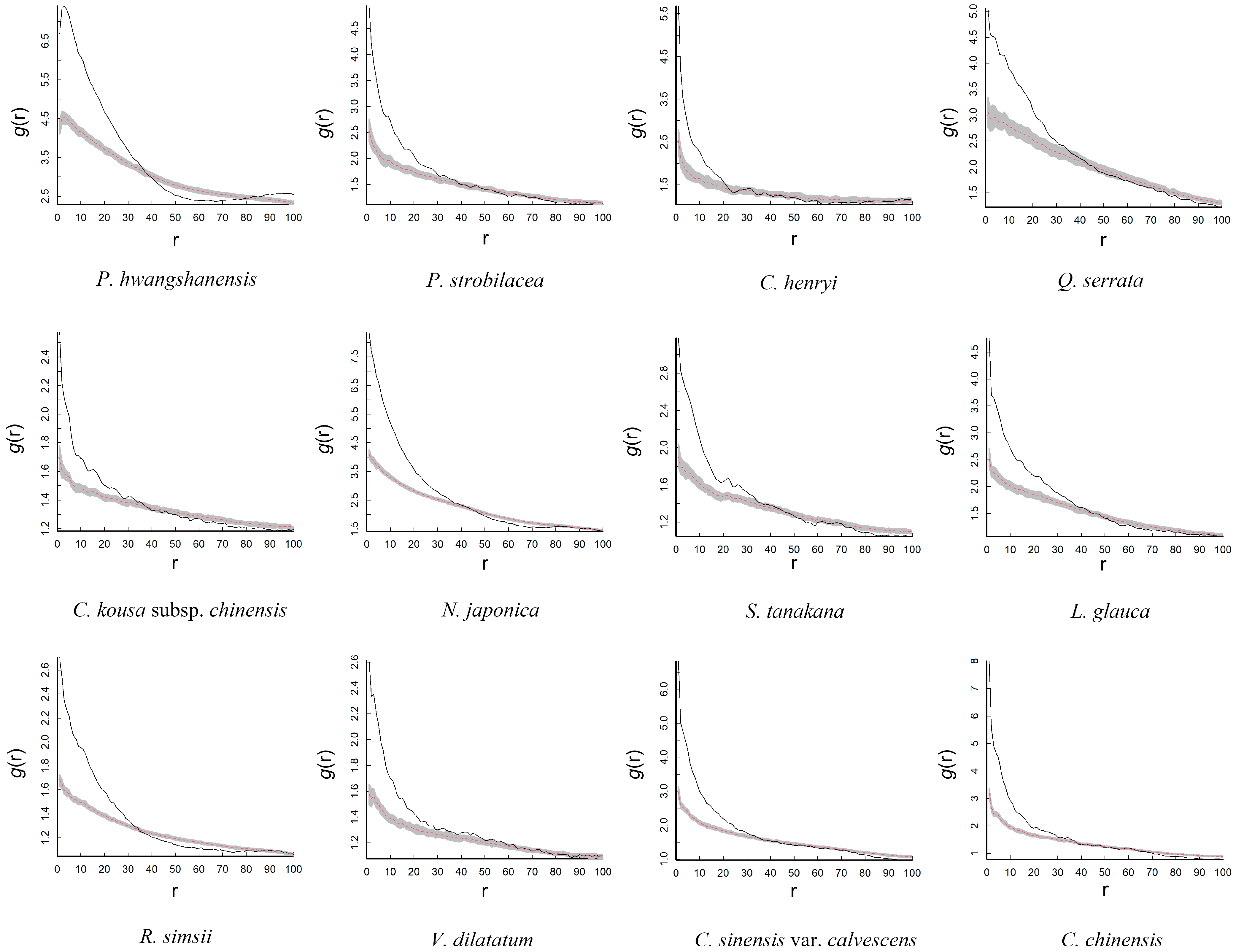
The analysis of the univariate g(r) function based on the CSR null model (Figure 3) revealed that the 12 dominant tree species exhibited a spatial pattern characterized by aggregated distribution throughout the study area. Furthermore, the degree of aggregation significantly decreased as the scale increased. The observed distribution of each tree species on the plot (Figure 2) was largely consistent with the spatial distribution patterns predicted by the CSR model. Therefore, when other influencing factors were not taken into account, the spatial distribution pattern of each dominant tree species primarily indicated an aggregated distribution. Additionally, we found that high-abundance species, such as P. hwangshanensis and R. simsii, exhibit greater distribution heterogeneity, which may be related to the effects of environmental filtering.
The HP null model revealed significant changes in the distribution pattern of each tree species after accounting for the effects of environmental heterogeneity (Figure 4). At scales below 40 m, the species displayed an aggregated distribution. However, as the scale increased, the distribution pattern transitioned to a random distribution (Table A1). After removing the effects of environmental factors, the aggregation scale of dominant species decreased or even shifted to a random distribution.

3.3. Intra-Specific and Inter-Specific Association

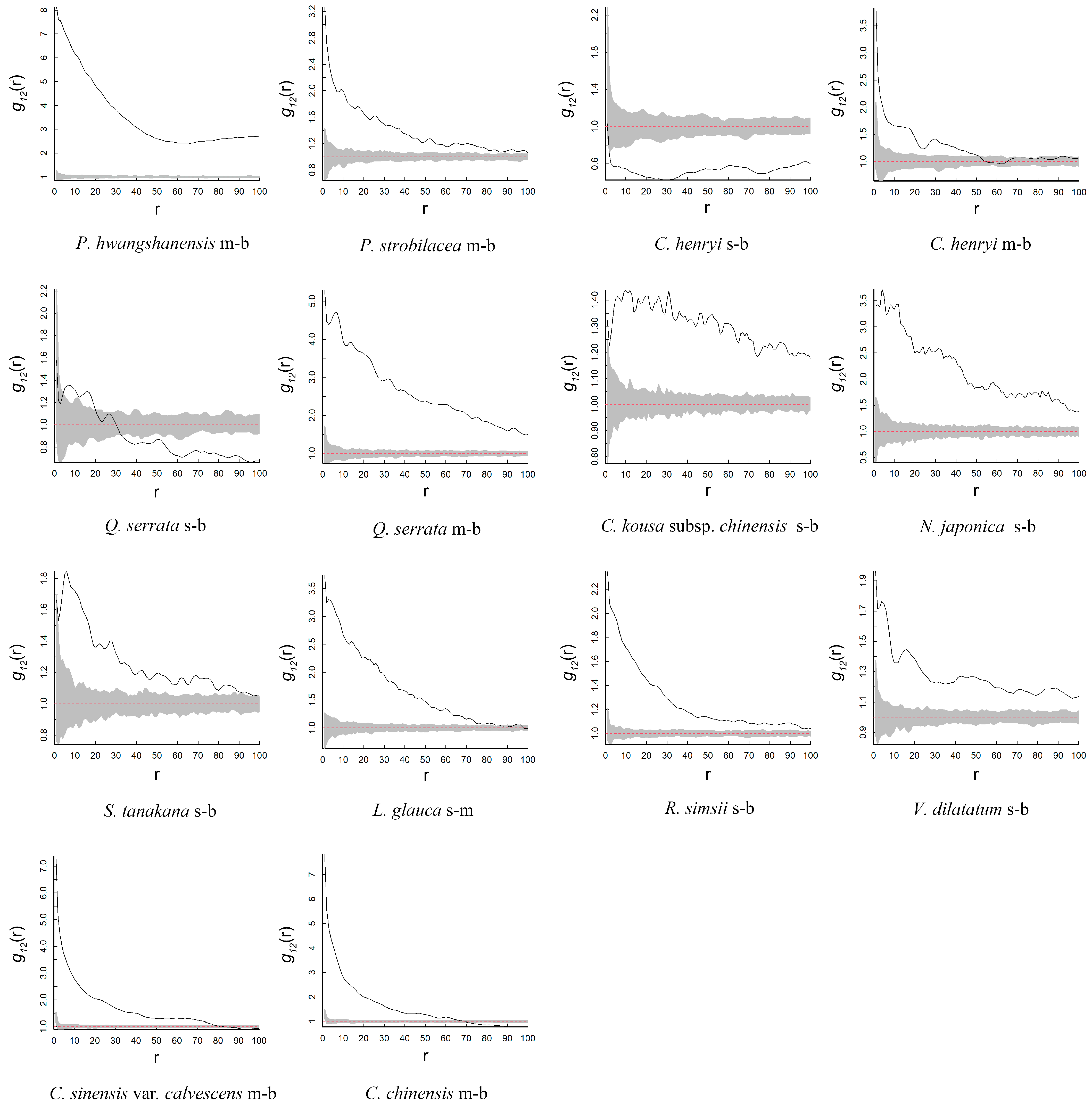
Based on the null models of CSR and AC, we analyzed the relationships between different life-history stages of the same tree species. Under CSR, many species, including P. hwangshanensis, P. strobilacea, Q. serrata, C. kousa subsp. chinensis, N. japonica, S. tanakana, R. simsii, and V. dilatatum, exhibited aggregation between their larger and smaller (or medium) individuals. Some species displayed aggregation at specific scales, followed by random distribution beyond those scales. However, few species showed negative associations between large and small individuals; for example, C. henryi demonstrated this pattern (Figure 5 and Table A2). This may indicate that most dominant tree species experience limitations due to restricted distributions, leading to aggregated distributions among their different life stages. The seeds of C. henryi are dispersed through zoochory, which involves animals and birds consuming the fruit and facilitating long-distance seed dispersal. This dispersal mechanism may help explain the observed negative spatial associations between conspecifics at different life stages.
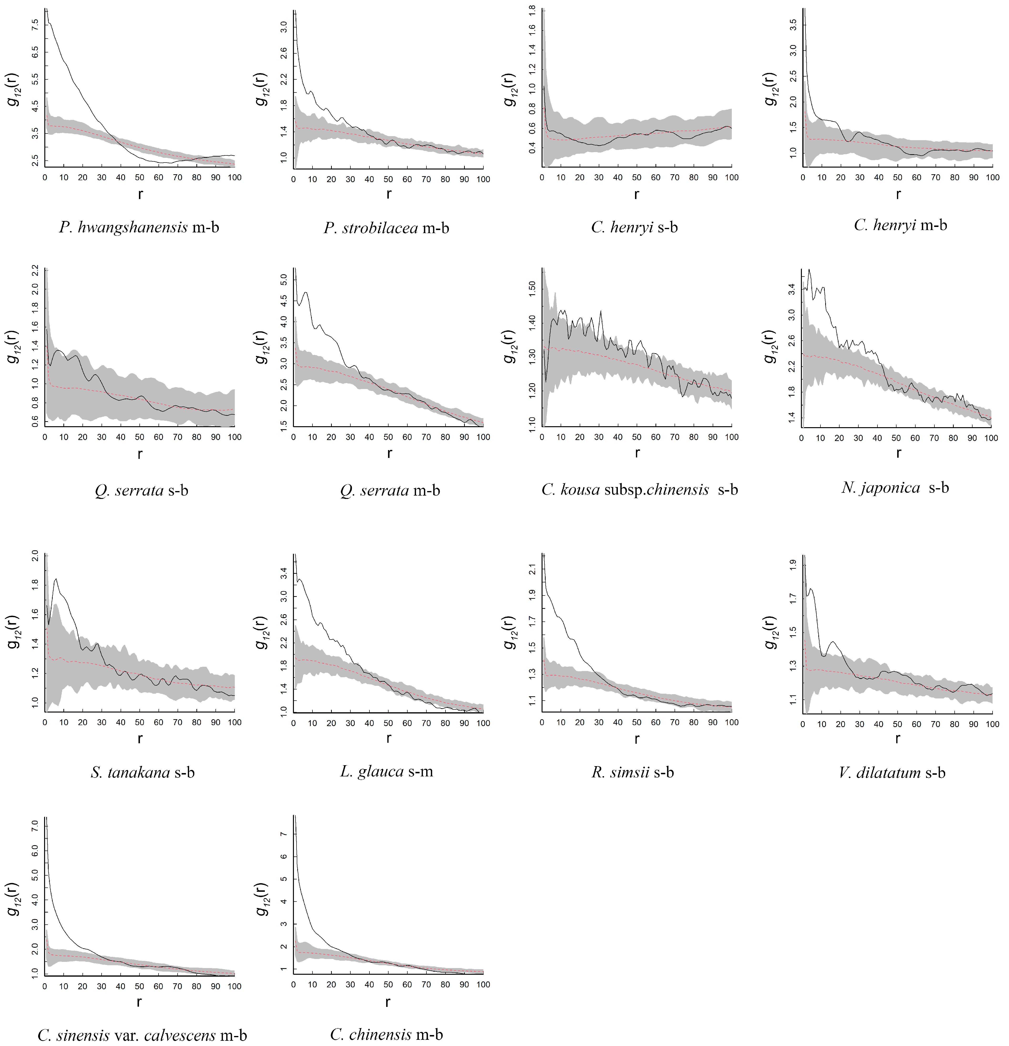
Under AC, when assessing the positions of large trees as a prerequisite condition, many small to medium tree species show an aggregated distribution around these large trees at limited scales. Beyond this point, their distribution becomes random. Notably, some species, including P. hwangshanensis, N. japonica, and R. simsii, exhibit negative associations with large trees at specific scales (Figure 6 and Table A2). This suggests that these species may experience significant intra-specific competition, particularly R. simsii, which has a very high density in this area and tends to cluster within the habitat.
We examined the relationship between large trees in the tree layer and small trees in the sub-arbor and shrub layers (see Table 3). Under CSR, P. hwangshanensis exhibited a distinct spatial relationship with each dominant species, owing to its notable high-altitude distribution characteristics. This species displayed either positive or negative associations with sub-arbor and shrub trees. In contrast, there was minimal correlation between the dominant species of P. strobilacea and C. henryi with sub-trees and shrubs, as these were mostly distributed randomly. Under AC, we found that small trees in the sub-arbor and shrub layers were positively associated with large trees in the tree layer.

3.4. Environment Factors and Species Distribution

Several soil and topographic variables were analyzed using PCA. For the soil factors, we selected four key variables that accounted for 66.98% of the cumulative proportion: total nitrogen (N), total carbon (C), gravel content (GO), and pH. All four topographic variables—mean elevation, slope, aspect, and convexity—were also retained in the analysis. The PCA results indicated that the first four principal components (PC1–PC4) explained 66.98% of the total variance (refer to Table A3). In PC1, we focused on N and C, which contributed 20.18% and 16.17%, respectively. In PC2, GO contributed 27.06%, while in PC3, pH made a significant contribution of 45.88% (Table A4). To examine the relationship between the spatial point patterns of dominant species and these environmental factors, we employed Berman’s test.
The results of Berman’s test showed associations between various topographic variables and the distribution of dominant species. P. hwangshanensis and R. simsii exhibited a strong positive correlation with elevation. In contrast, N. japonica prefers steep slopes, while C. chinensis thrives on flat slopes. On the Lushan plot, Q. serrata, S. tanakana, and L. glauca favor the northern aspect. Additionally, P. hwangshanensis, S. tanakana, R. simsii, and C. chinensis tend to grow in low convex areas, such as mountaintops or valleys, whereas N. japonica prefers undulating planes (see Table 4). Regarding soil physicochemical properties, soil N and C are indicators of soil nutrition, which are considered important for plant growth. However, many species showed a negative association with soil N and C. Only L. glauca favored soil with high nutritional content. Most species prefer soil with low gravel content, but L. glauca shows a preference for rocky soil. The pH results indicated that the soil in this plot is generally acidic, and R. simsii, in particular, thrives in acidic soil (Table 5).

4. Discussion

4.1. The Processes Shaping Species Distribution Patterns

Species distribution patterns can be influenced by a variety of factors. At small scales, it is common for populations to cluster due to seed dispersal limitations [34]. At larger scales, the distribution is more influenced by environmental heterogeneity, including factors such as elevation, convexity, and soil characteristics [11,12]. Research has shown that in subtropical forests, even when environmental heterogeneity is present, seed dispersal limitation plays a significant role in determining the extent of stump clumping [35]. Therefore, we speculate that the spatial distribution of the dominant tree species observed in the plot is primarily shaped by both environmental heterogeneity and seed dispersal limitations [36,37].
The distribution patterns of the 12 dominant tree species examined in this study displayed clear scale-dependent characteristics. At smaller scales, the species formed aggregated distributions, which transitioned to random patterns as the spatial scale increased. This observation aligns with theoretical expectations, suggesting that dispersal limitation primarily drives fine-scale aggregation, while environmental heterogeneity becomes increasingly significant at larger scales [14,38]. The results from the HP model, which took environmental variation into account, indicated that dispersal limitation alone could explain aggregation patterns for most species at scales below 40 m. We propose that dispersal limitation may have contributed to the initial spatial aggregation of seeds at smaller scales.
Species with limited seed dispersal capabilities, such as P. hwangshanensis and C. henryi, exhibited significant small-scale clustering. This observation aligns with findings from tropical forest ecosystems, where dispersal limitation is recognized as a key factor influencing spatial structure [14]. Additionally, when controlling for environmental heterogeneity, we observed a reduction in aggregation intensity at larger scales. This suggests that topographic factors, particularly elevation and slope, as well as soil properties, especially total nitrogen and carbon content, increasingly influence species distributions as the spatial scale expands [39,40].

4.2. Interpreting the Patterns of Intra- and Inter-Specific Associations

In the CSR null model, individuals at different life stages within the same tree species exhibited aggregation, particularly evident in sub-tree and shrub species. However, large and small trees of C. henryi and Q. serrata displayed segregation under the CSR null model. When using the AC null model, the degree of aggregation between large and small trees of the same species significantly decreased. Most of these trees were grouped at distances less than 40 m, but beyond this range, they tended to show random distributions, with very few instances of exclusion occurring at a larger scale. An analysis of intra-specific associations highlighted the complex relationships among different life stages of the same species. Under CSR assumptions, most species demonstrated positive associations between adult and juvenile trees, especially among shrub-layer species like R. simsii. In contrast, when applying the AC model, which fixes adult tree positions, these positive associations were largely confined to distances of less than 40 m.
These findings provide partial empirical support for the Janzen-Connell hypothesis; however, further research is necessary to untangle the potential confounding effects of dispersal limitation and environmental filtering [7,17]. The scale-dependent nature of these intra-specific interactions indicates that different ecological processes may dominate at various spatial scales. Specifically, facilitation might occur at very small scales, while competitive exclusion could become more pronounced at intermediate distances [41].
Inter-specific association patterns revealed complex dynamics among species. The canopy species P. hwangshanensis displayed particularly strong spatial relationships with other species, demonstrating both positive and negative associations. The observed associations suggest that environmental filtering along elevation gradients could be a primary influencing factor. In contrast, other dominant canopy species, such as C. henryi, showed more random spatial relationships with understory species. When we accounted for the fixed positions of canopy trees using the AC model, many species exhibited positive associations between canopy trees and understory saplings at smaller scales. This supports theories of species coexistence through spatial niche partitioning [42] and the hypothesis of species herd protection [43]. These findings suggest that while environmental heterogeneity creates broad-scale distribution patterns, fine-scale biotic interactions—encompassing both facilitation and competition—play a significant role in maintaining species diversity within this forest ecosystem [38,44].

4.3. Drivers of Species Distribution: An Environmental Perspective

Many species surprisingly showed negative associations with high-nutrient soils. This may reflect either competitive exclusion by more nutrient-demanding species or adaptive strategies that help them thrive in poorer soils. The species exhibited distinct microhabitat preferences: N. japonica preferred steep slopes, S. tanakana favored north-facing slopes, and R. simsii showed a strong preference for acidic soils. These specialized habitat requirements likely contribute to species coexistence by reducing niche overlap [45]. Additionally, several dominant species were associated with low convexity areas, such as mountaintops and valleys, while others preferred more undulating terrain. This further emphasizes the importance of microtopographic variation in maintaining community diversity [46,47].
The current study has several limitations that suggest important avenues for future research. Firstly, while dispersal limitation was inferred from spatial patterns, obtaining direct measurements of seed dispersal distance for the dominant species would enhance these interpretations. Secondly, since this is a cross-sectional study, it could be complemented by longitudinal data to understand better how spatial patterns evolve over time during forest succession. Lastly, incorporating functional trait data, such as seed size and wood density, may help to explain the observed distribution patterns.

4.4. Management Implications in Deciduous Forests

The study of plant spatial patterns is essential for understanding community assembly and species coexistence mechanisms in deciduous forests. Insights gained from this research can directly inform improved management and conservation strategies. Dispersal limitation is a key initial factor influencing spatial patterns, though enrichment planting offers a potential solution to mitigate its effects. In deciduous forests, intra- and inter-specific competition is generally less intense, allowing species to exhibit habitat reliance. From a management perspective, targeted thinning and the creation of forest gaps in appropriate locations can promote the regeneration and growth of specific species, thereby enhancing forest structure and biodiversity.

5. Conclusions

In conclusion, this study demonstrates that the spatial structure of Lushan Mountain’s deciduous broad-leaved forest emerges from the interplay of multiple ecological processes acting across spatial scales. Dispersal limitation creates initial aggregation at fine scales, while environmental heterogeneity sorts species across the landscape. Biotic interactions, including both competitive exclusion and facilitation, further modify these patterns at intermediate scales. These findings advance our understanding of subtropical forest ecology by illustrating how the interplay between neutral processes (e.g., dispersal limitation) and niche-based mechanisms (e.g., environmental filtering and biotic interactions) shapes community assembly. From an applied perspective, these results suggest that forest management and restoration efforts should account for both landscape-scale environmental heterogeneity and fine-scale biotic interactions to maintain ecosystem diversity and function.

Author Contributions

Conceptualization, J.W. and J.Z.; Data curation, J.W., Z.X., D.X. and Z.Z.; Formal analysis, J.W.; Funding acquisition, J.Z.; Investigation, J.W., Z.X., D.X., Z.Z., S.Z. and J.Z.; Project administration, S.Z. and J.Z.; Resources, D.X. and Z.Z.; Writing—original draft, J.W.; Writing—review and editing, Z.X., S.Z. and J.Z. All authors have read and agreed to the published version of the manuscript.

Funding

This work was supported by Special Grants of the Lushan Botanical Garden, Chinese Academy of Sciences (2024ZWZX15) and Jiangxi Provincial Natural Science Foundation (20242BAB20261).

Data Availability Statement

The data are available within the article.

Conflicts of Interest

The authors declare no conflicts of interest.

Appendix A

Table A1. Summary of g(r) function results of 12 dominant species under CSR and HP.
Species CSR HP
P. hwangshanensis+ at all scales+ before 40 m, − at 40–80 m, after that, r
P. strobilacea+ at all scales, + decrease with the scale increase+ before 35 m, after that, r
C. henryi+ at all scales, 60–80 m, r+ before 20 m, after that, r
Q. serrata+ at all scales, + decrease with the scale increase+ before 40 m, after that, r
C. kousa subsp. chinensis+ at all scales+ before 35 m, after that, r
N.japonica+ at all scales+ before 40 m, − at 40–80 m, after that, r
S. tanakana+ at all scales, + decrease with the scale increase+ before 35 m, after that, r
L. glauca+ at all scales+ before 40 m, after that, r
R. simsii+ at all scales+ before 35 m, − between 40 and 80 m, after that, r
V. dilatatum+ at all scales+ before 50 m, after that, r
C. sinensis var. calvescens+ at all scales, r after 90 m+ before 35 m, after that, r
C. chinensis+ before 70 m, after that, −+ before 40 m, r between 40 and 70 m, after that, −
“+” represents aggregated distribution, “−” represents segregation distribution, and “r” represents random distribution.
Table A2. Summary of g12 (r) function results between big or medium individuals and smaller ones of 12 dominant species under CSR and AC.
Species CSR AC
P. hwangshanensis (b-m)+ at all scales+ before 35 m, − between 35 and 80 m, after that, r
P. strobilacea (b-m)+ at all scales+ before 35 m, after that, r
C. henryi (b-s)r before 5 m, after that, −+ at all scales
C. henryi (b-m)+ before 52 m, after that, r+ before 20 m, after that, r
Q. serrata (b-s)+ before 20 m, 20–30 m, r, after that, −+ at all scales
Q. serrata (b-m)+ at all scales+ before 35 m, after that, r
C. kousa subsp. chinensis (b-s)+ at all scales+ at all scales
C. kousa subsp. chinensis (b-m)+ at all scales+ before 40 m, after that, r
N. japonica (b-s)+ at all scales+ before 42 m, after that, r
N. japonica (b-m)+ at all scales+ before 40 m, − between 40 and 80 m, after that, r
S. tanakana (b-s)+ at all scales+ before 20 m, after that, r
S. tanakana (b-m)+ before 85 m, after that, r+ before 25 m, r between 25 and 80 m, after that, −
L. glauca (m-s)+ before 85 m, after that, r+ before 35 m, after that, r
R. simsii (b-s)+ at all scales− before 35 m, after that, r
R. simsii (m-s)+ at all scales− before 35 m, after that, r
V. dilatatum (b-s)+ at all scales+ before 22 m, after that, r
V. dilatatum (m-s)+ at all scales+ before 22 m, after that, r
C. sinensis var. calvescens (b-m)+ before 80 m, after that, r+ before 35 m, r between 35 and 75 m, after that, −
C. chinensis (b-m)+ before 70 m, after that, −+ before 30 m, after that, r
“+” represents aggregated distribution, “−” represents segregation distribution, and “r” represents random distribution.
Table A3. Importance of components in PCA.
Standard Deviation Proportion of Variance Cumulative Proportion
PC11.98490.30310.3031
PC21.57810.19160.4946
PC31.11350.09540.5900
PC41.01870.07980.6698
PC50.98600.07480.7446
PC60.90080.06240.8070
Table A4. Summary of soil factors contribution of PC1–PC6.
Soil Factors PC1 PC2 PC3 PC4 PC5 PC6
pH value2.242.1845.880.9411.125.46
Total Nitrogen20.181.592.270.012.170.92
Total Carbon16.173.2211.050.020.200.09
Total Phosphorus8.681.332.961.960.0715.32
Total Potassium2.331.858.7918.5727.7324.48
Alkaline Hydrolyzable Nitrogen10.333.097.922.000.120.01
Available Phosphorus12.850.050.800.052.328.89
Available Potassium14.290.886.611.620.460.02
Soil Moisture Content1.1220.834.2410.210.660.58
Bulk Density1.075.481.1462.220.366.48
Gravel Content5.1327.062.950.024.250.04
Root Content0.385.712.552.3745.7137.72
Soil Content5.2226.732.860.024.830.01

References

  1. Lu, F.; Wang, B.; Li, J.X.; Li, D.X.; Liu, S.Y.; Guo, Y.L.; Huang, F.Z.; Xiang, W.S.; Li, X.K. Both Biotic and Abiotic Factors Shape the Spatial Distribution of Aboveground Biomass in a Tropical Karst Seasonal Rainforest in South China. Forests 2004, 15, 1904. [Google Scholar] [CrossRef]
  2. Wei, J.X.; Yang, L.S.; Jiang, Z.G.; Yao, H.; Yu, H.L.; Luo, F.L.; Qiao, X.J.; Xu, Y.Z.; Jiang, M.X. Spatial Distribution and Intraspecific and Interspecific Associations of Dominant Tree Species in a Deciduous Broad-Leaved Forest in Shennongjia, China. Diversity 2025, 17, 335. [Google Scholar] [CrossRef]
  3. Zhang, L.Y.; Dong, L.B.; Liu, Q.; Liu, Z.G. Spatial patterns and interspecific associations during natural regeneration in three types of secondary forest in the central part of the Greater Khingan Mountains, Heilongjiang Province, China. Forests 2020, 11, 152. [Google Scholar] [CrossRef]
  4. Wiegand, T.; Wang, X.G.; Anderson-Teixeira, K.J.; Bourg, N.A.; Cao, M.; Ci, X.Q.; Davies, S.J.; Hao, Z.Q.; Howe, R.W.; Kress, W.J.; et al. Consequences of spatial patterns for coexistence in species-rich plant communities. Nat. Ecol. Evol. 2021, 5, 965–973. [Google Scholar] [CrossRef]
  5. Yang, X.Q.; Yan, H.B.; Li, B.H.; Han, Y.Z.; Song, B. Spatial distribution patterns of Symplocos congeners in a subtropical evergreen broad-leaf forest of southern China. J. For. Res. 2018, 29, 773–784. [Google Scholar] [CrossRef]
  6. Guo, Y.L.; Lu, J.M.; Franklin, S.B.; Wang, Q.G.; Xu, Y.Z.; Zhang, K.H.; Bao, D.C.; Qiao, X.J.; Huang, H.D.; Lu, Z.J.; et al. Spatial distribution of tree species in a species-rich subtropical mountain forest in central China. Can. J. For. Res. 2013, 43, 826–835. [Google Scholar] [CrossRef]
  7. Cheng, J.J.; Mi, X.C.; Nadrowski, K.; Ren, H.B.; Zhang, J.T.; Ma, K.P. Separating the effect of mechanisms shaping species abundance distributions at multiple scales in a subtropical forest. Oikos 2013, 121, 236–244. [Google Scholar] [CrossRef]
  8. Baldeck, C.A.; Harms, K.E.; Yavitt, J.B.; John, R.; Turner, B.L.; Valencia, R.; Navarrete, H.; Bunyavejchewin, S.; Kiratiprayoon, S.; Yaacob, A.; et al. Habitat filtering across tree life stages in tropical forest communities. Proc. R. Soc. B Biol. Sci. 2013, 280, 20130548. [Google Scholar] [CrossRef]
  9. Yuan, Z.Q.; Gazol, A.; Wang, X.G.; Xing, D.L.; Lin, F.; Bai, X.J.; Zhao, Y.Q.; Li, B.H.; Hao, Z.Q. What happens below the canopy? Direct and indirect influences of the dominant species on forest vertical layers. Oikos 2012, 121, 1145–1153. [Google Scholar] [CrossRef]
  10. Zhang, Y.T.; Li, J.M.; Chang, S.L.; Li, X.; Lu, J.J. Spatial distribution pattern of Picea schrenkiana population in the Middle Tianshan Mountains and the relationship with topographic attributes. J. Arid Land 2012, 4, 457–468. [Google Scholar] [CrossRef]
  11. Lan, G.Y.; Hu, Y.H.; Cao, M.; Zhu, H. Topography related spatial distribution of dominant tree species in a tropical seasonal rain forest in China. For. Ecol. Manag. 2011, 262, 1507–1513. [Google Scholar] [CrossRef]
  12. Zhang, Z.H.; Hu, G.; Ni, J. Effects of topographical and edaphic factors on the distribution of plant communities in two subtropical karst forests, southwestern China. J. Mt. Sci. 2013, 10, 95–104. [Google Scholar] [CrossRef]
  13. Hao, Z.Q.; Zhang, J.; Song, B.; Ye, J.; Li, B.H. Vertical structure and spatial associations of dominant tree species in an old-growth temperate forest. For. Ecol. Manag. 2007, 252, 1–11. [Google Scholar] [CrossRef]
  14. Hu, Y.H.; Sha, L.Q.; Blanchet, F.G.; Zhang, J.L.; Tang, Y.; Lan, G.Y.; Cao, M. Dominant species and dispersal limitation regulate tree species distributions in a 20-ha plot in Xishuangbanna, southwest China. Oikos 2012, 121, 952–960. [Google Scholar] [CrossRef]
  15. Zhu, Y.; Mi, X.C.; Ren, H.B.; Ma, K.P. Density dependence is prevalent in a heterogeneous subtropical forest. Oikos 2010, 119, 109–119. [Google Scholar] [CrossRef]
  16. Jiao, J.J.; Wu, C.P.; Jiang, B.; Wang, Z.G.; Yuan, W.G.; Zhu, J.R.; Li, T.T.; Yang, S.Z.; Yan, L.J. Negative density restricts the coexistence and spatial distribution of dominant species in subtropical evergreen broad-leaved forests in China. Forests 2022, 13, 1227. [Google Scholar] [CrossRef]
  17. Zhu, Y.; Mi, X.C.; Ma, K.P. A mechanism of plant species coexistence: The negative density-dependent hypothesis. Biodivers. Sci. 2009, 17, 594–604. [Google Scholar] [CrossRef]
  18. Benot, M.L.; Bittebiere, A.K.; Ernoult, A.; Clement, B.; Mony, C. Fine-scale spatial patterns in grassland communities depend on species clonal dispersal ability and interactions with neighbours. J. Ecol. 2013, 101, 626–636. [Google Scholar] [CrossRef]
  19. Beyns, R.; Bauman, D.; Drouet, T. Fine-scale tree spatial patterns are shaped by dispersal limitation which correlates with functional traits in a natural temperate forest. J. Veg. Sci. 2021, 32, e13070. [Google Scholar] [CrossRef]
  20. Wolf, A. Fifty year record of change in tree spatial patterns within a mixed deciduous forest. For. Ecol. Manag. 2005, 215, 212–223. [Google Scholar] [CrossRef]
  21. Chaturvedi, R.K.; Raghubanshi, A.S.; Singh, J.S. Plant functional traits with particular reference to tropical deciduous forests: A review. J. Biosci. 2011, 36, 963–981. [Google Scholar] [CrossRef]
  22. Wang, L.; He, Y.; Umer, M.; Guo, Y.; Tian, Q.Y.; Kang, L.L.; Fang, Z.Y.; Shen, K.P.; Xia, T.T.; Wu, P.; et al. Strategic differentiation of subcommunities composed of evergreen and deciduous woody species associated with leaf functional traits in the subtropical mixed forest. Ecol. Indic. 2023, 150, 110281. [Google Scholar] [CrossRef]
  23. Lu, R.K.; Zhu, H.Z.; He, P.A.; Chen, C.Z.; Chen, H.M.; Zhou, J.M.; Su, D.C.; Xu, J.M.; Qin, H.Y.; Bao, S.D.; et al. Analytical Methods for Soil and Agro-Chemistry; China Agricultural Science and Technology Press: Beijing, China, 2000. [Google Scholar]
  24. He, C.M.; Jia, S.H.; Luo, Y.; Hao, Z.Q.; Yin, Q.L. Spatial distribution and species association of dominant tree species in Huangguan Plot of Qinling Mountains, China. Forests 2022, 13, 866. [Google Scholar] [CrossRef]
  25. Ben-Said, M. Spatial point-pattern analysis as a powerful tool in identifying pattern-process relationships in plant ecology: An updated review. Ecol. Process. 2021, 10, 56. [Google Scholar] [CrossRef]
  26. Wiegand, T.; Moloney, K.A. Rings, circles, and null models for point pattern analysis in ecology. Oikos 2004, 104, 209–229. [Google Scholar] [CrossRef]
  27. Carrer, M.; Castagneri, D.; Popa, I.; Pividori, M.; Lingua, E. Tree spatial patterns and stand attributes in temperate forests: The importance of plot size, sampling design, and null model. For. Ecol. Manag. 2018, 407, 125–134. [Google Scholar] [CrossRef]
  28. Baddeley, A.; Rubak, E.; Turner, R. Spatial Point Patterns: Methodology and Applications with R; CRC Press: Boca Raton, FL, USA, 2016. [Google Scholar]
  29. Berman, M. Testing for spatial association between a point process and another stochastic process. J. R. Stat. Soc. Ser. C Appl. Stat. 1986, 5, 54–62. [Google Scholar] [CrossRef]
  30. Baddeley, A.; Turner, R. Spatstat: An R package for analyzing spatial point patterns. J. Stat. Softw. 2005, 12, 1–42. [Google Scholar] [CrossRef]
  31. Baddeley, A. Analysing spatial point patterns in R[C]//Workshop Notes. 2008. Available online: https://d1wqtxts1xzle7.cloudfront.net/52438478/baddeley2010-spatial_point_pattern_analysis-libre.pdf?1491178707=&response-content-disposition=inline%3B+filename%3DAnalysing_spatial_point_patterns_in_R.pdf&Expires=1758550582&Signature=gfOuzE-qYmM5AulBDe~OwnMKLED9QaUZK~5MR8tZzkfroLvAdvDuT2Q~PRJtduh2fcSvktskYDyRaDHnGCYTOqWFKkfUPuDFd-gCUIhznWM~24BvoSgaZnAVEexRIfly8p4TNj41aYG6eui-auNCm5g7oai9fUgXO5y2EoUfHgdj5ZXelbmg6WIClMoMcdRmGEqZVR1DS2udAkNzUpiDMpwHIsaKusvtbN7w8I-TU7TSZGqHCgXCXLpw2J16RfDBzMjVr2DhWRmppS1Pnbqg6R86tbadiVOMkM9cCq~QQ0S-D97Z9-GHFKLPSJGOFv9cXaeoBMNBMuYd8TPiygWvKA__&Key-Pair-Id=APKAJLOHF5GGSLRBV4ZA (accessed on 20 September 2025).
  32. Pijl, L.V.D. Principles of Dispersal in Higher Plants. Q. Rev. Biol. 1970, 72, 499. [Google Scholar]
  33. Wu, Z.Y.; Raven, P.H.; Hong, D.Y.; Li, D.Z.; Boufford, D.E.; Peter, H.; Brach, A.R.; Stuessy, T.F.; Lang, K.Y.; Gilbert, M.G.; et al. Flora of China; Science Press: Beijing, China; Missouri Botanical Garden Press: St. Louis, MO, USA, 2010. [Google Scholar]
  34. Perea, A.J.; Wiegand, T.; Garrido, J.L.; Rey, P.J.; Alcántara, J.M. Legacy effects of seed dispersal mechanisms shape the spatial interaction network of plant species in Mediterranean forests. J. Ecol. 2021, 109, 3670–3684. [Google Scholar] [CrossRef]
  35. Zhang, Z.H.; Hu, G.; Zhu, J.D.; Ni, J. Aggregated spatial distributions of species in a subtropical karst forest, southwestern China. J. Plant Ecol. 2013, 6, 131–140. [Google Scholar] [CrossRef]
  36. Getzin, S.; Wiegand, T.; Wiegand, K.; He, F.L. Heterogeneity influences spatial patterns and demographics in forest stands. J. Ecol. 2008, 96, 807–820. [Google Scholar] [CrossRef]
  37. Shen, G.C.; He, F.L.; Waagepetersen, R.; Sun, I.F.; Hao, Z.Q.; Chen, Z.S.; Yu, M.J. Quantifying effects of habitat heterogeneity and other clustering processes on spatial distributions of tree species. Ecology 2013, 94, 2436–2443. [Google Scholar] [CrossRef] [PubMed]
  38. Lv, T.; Zhao, R.; Wang, N.J.; Xie, L.; Feng, Y.Y.; Li, Y.; Ding, H.; Fang, Y.M. Spatial distributions of intra-community tree species under topographically variable conditions. J. Mt. Sci. 2023, 20, 391–402. [Google Scholar] [CrossRef]
  39. Wan, J.Z.; Yu, J.H.; Yin, G.J.; Song, Z.M.; Wei, D.X.; Wang, C.J. Effects of soil properties on the spatial distribution of forest vegetation across China. Glob. Ecol. Conserv. 2019, 18, e00635. [Google Scholar] [CrossRef]
  40. Zhao, H.; Wang, Q.R.; Fan, W.; Song, G.H. The relationship between secondary forest and environmental factors in the southern Taihang Mountains. Sci. Rep. 2017, 7, 16431. [Google Scholar] [CrossRef]
  41. Zhang, J.; Hao, Z.Q.; Song, B.; Li, B.H.; Wang, X.G.; Ye, J. Fine-scale species co-occurrence patterns in an old-growth temperate forest. For. Ecol. Manag. 2009, 257, 2115–2120. [Google Scholar] [CrossRef]
  42. Hou, J.H.; Mi, X.C.; Liu, C.R.; Ma, K.P. Spatial patterns and associations in a Quercus-Betula forest in northern China. J. Veg. Sci. 2004, 15, 407–414. [Google Scholar] [CrossRef]
  43. Peters, H.A. Neighbour-regulated mortality: The influence of positive and negative density dependence on tree populations in species-rich tropical forests. Ecol. Lett. 2010, 6, 757–765. [Google Scholar] [CrossRef]
  44. Zhou, Q.; Shi, H.; Shu, X.; Xie, F.L.; Zhang, K.R.; Zhang, Q.F.; Dang, H.S. Spatial distribution and interspecific associations in a deciduous broad-leaved forest in north-central China. J. Veg. Sci. 2019, 30, 1153–1163. [Google Scholar] [CrossRef]
  45. Luo, Z.R.; Yu, M.J.; Chen, D.L.; Wu, Y.G.; Ding, B.Y. Spatial associations of tree species in a subtropical evergreen broad-leaved forest. J. Plant Ecol. 2012, 5, 346–355. [Google Scholar] [CrossRef]
  46. Du, H.; Peng, W.X.; Song, T.Q.; Zeng, F.P.; Wang, K.L.; Song, M.; Zhang, H. Spatial pattern of woody plants and their environmental interpretation in the karst forest of southwest China. Plant Biosyst. 2015, 149, 121–130. [Google Scholar] [CrossRef]
  47. Omelko, A.; Ukhvatkina, O.; Zhmerenetsky, A.; Sibirina, L.; Petrenko, T.; Bobrovsky, M. From young to adult trees: How spatial patterns of plants with different life strategies change during age development in an old-growth Korean pine-broadleaved forest. For. Ecol. Manag. 2018, 411, 46–66. [Google Scholar] [CrossRef]
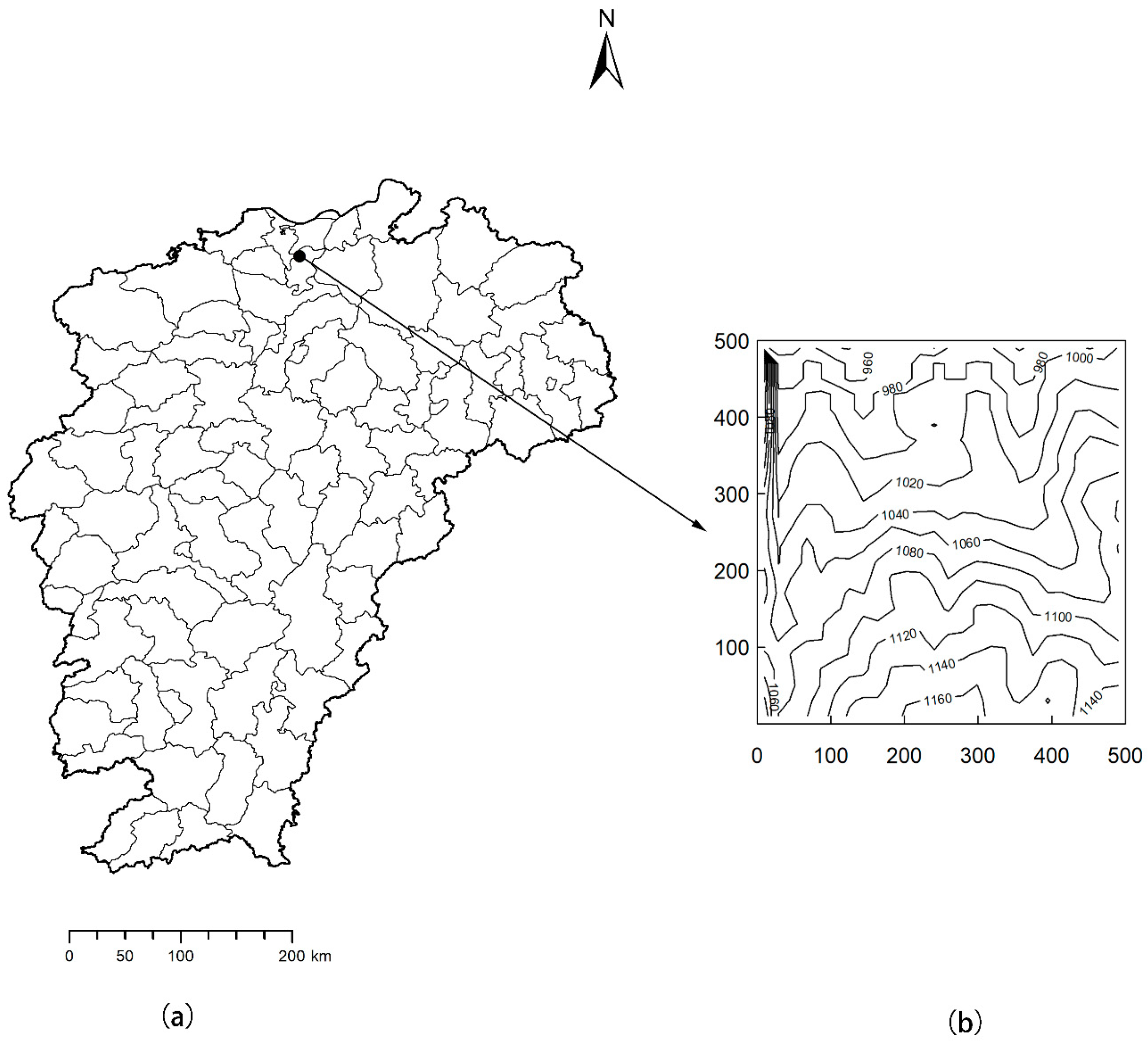
Figure 1. Position of Lushan Mountain 25 ha deciduous broad-leaved forest plot in Jiangxi Province (a) and topography of the plot ((b), in meters).
Forests 16 01511 g001
Figure 2. Spatial distribution plot of 12 dominant species, with all individuals divided into three classes and marked with different colors and shapes; units given in meters.
Forests 16 01511 g002
Figure 3. g(r) function analysis of dominant tree species under CSR. The solid black line represents the observed value of g(r), the red dashed line represents the theoretical value of g(r), and the gray area indicates the 98% confidence interval. If the solid black line is above the confidence interval area, the aggregation pattern can be judged; if the solid black line is between the confidence interval area, random distribution can be judged; the solid black line below the confidence interval indicates separation distribution mode. Spatial scale (r; m) represents interplant distance.
Forests 16 01511 g003
Figure 4. g(r) function analysis of dominant tree species under HP. The solid black line represents the observed value of g(r), the red dashed line represents the theoretical value of g(r), and the gray area indicates the 98% confidence interval. If the solid black line is above the confidence interval area, the aggregation pattern can be judged; if the solid black line is between the confidence interval area, random distribution can be judged; the solid black line below the confidence interval indicates separation distribution mode. Spatial scale (r; m) represents interplant distance.
Forests 16 01511 g004
Figure 5. g12(r) function results between big or medium individuals and smaller ones of 12 dominant species under CSR; “b” represents big individuals, “m” represents medium individuals, and “s” represents small individuals. The solid black line represents the observed value of g(r), the red dashed line represents the theoretical value of g(r), and the gray area indicates the 98% confidence interval. If the solid black line is above the confidence interval area, the aggregation pattern can be judged; if the solid black line is between the confidence interval area, random distribution can be judged; the solid black line below the confidence interval indicates the separation distribution mode. Spatial scale (r; m) represents interplant distance.
Forests 16 01511 g005
Figure 6. g12 (r) function results between big or medium individuals and smaller ones of 12 dominant species under AC. The solid black line represents the observed value of g(r), the red dashed line represents the theoretical value of g(r), and the gray area indicates the 98% confidence interval. If the solid black line is above the confidence interval area, the aggregation pattern can be judged; if the solid black line is between the confidence interval area, random distribution can be judged; the solid black line below the confidence interval indicates the separation distribution mode. Spatial scale (r; m) represents interplant distance.
Forests 16 01511 g006
Table 1. Taxonomic and ecological characteristics of 12 dominant species.
SpeciesFamilyAbundanceFruit TypeDispersal Mode
Pinus hwangshanensis W. Y. HsiaPinaceae3099NutGravity; animal
Platycarya strobilacea Siebold & Zucc.Juglandaceae1676SamaraWind
Castanea henryi (Skan) Rehder & E. H. WilsonFagaceae849NutGravity; animal
Quercus serrata Thunb.Fagaceae1480NutGravity; animal
Cornus kousa subsp. chinensis (Osborn) Q. Y. XiangCornaceae5434AggregateGravity; animal
Neoshirakia japonica (Siebold & Zucc.) EsserEuphorbiaceae4828CapsuleAnimal
Symplocos tanakana NakaiSymplocaceae2158DrupeGravity; animal
Lindera glauca (Siebold & Zucc.) BlumeLauraceae2492DrupeGravity; animal
Rhododendron simsii Planch.Ericaceae28,433CapsuleWind; animal
Viburnum dilatatum Thunb.Viburnaceae4126DrupeGravity; animal
Corylopsis sinensis var. calvescens Rehder & E. H. WilsonHamamelidaceae3501CapsuleGravity; animal
Corylopsis sinensis Hemsl.Hamamelidaceae3256CapsuleGravity; animal
Table 2. Abundance and life stages of 12 dominant species.
SpeciesLayerSmall Trees
Proportion (%)
Medium Trees
Proportion (%)
Big Trees
Proportion (%)
P. hwangshanensisTree1.1631.6967.15
P. strobilaceaTree2.5768.4429.00
C. henryiTree19.7931.6848.53
Q. serrataTree19.1257.5723.31
C. kousa subsp. chinensisSub-arbor59.6626.6313.71
N. japonicaSub-arbor77.5920.731.68
S. tanakanaSub-arbor32.6247.6419.74
L. glaucaSub-arbor84.8314.930.24
R. simsiiShrub8.6245.8045.59
V. dilatatumShrub15.8561.5122.64
C. sinensis var. calvescensShrub1.6610.3787.97
C. chinensisShrub2.9212.8784.21
Table 3. Summary of g12 (r) function results between big tree layers individuals and small individuals of sub-arbor and common shrubs under CSR and AC.
SpeciesCSRAC
P. hwangshanensis–C. kousa subsp. chinensis + at all scales+ before 28 m, after that, r
P. hwangshanensis–N. japonica− at all scales+ before 45 m, after that, r
P. hwangshanensis–S. tanakana+ at all scalesr at all scales
P. hwangshanensis–L. glauca− at all scalesr at all scales
P. hwangshanensis–R. simsii+ at all scales+ before 30 m and 80–100 m,
r between 30 and 38 m and 70–80 m,
− between 38 and 70 m
P. hwangshanensis–V. dilatatum− before 38 m, r between 38 and 40 m,
after that, +
− before 30 m, after that, r
P. hwangshanensis–C. sinensis var. calvescens− at all scales− between 7 and 17 m, r at other scales
P. strobilacea–C. kousa subsp. chinensis + before 55 m, after that, rr at all scales
P. strobilacea–N. japonica+ at all scales+ before 40 m, after that, r
P. strobilacea–S. tanakanar at all scalesr at all scales
P. strobilacea–L. glauca+ before 55 m, after that, r+ before 35 m, after that, r
P. strobilacea–R. simsii+ between 30 and 62 m,
r between 0 and 30 m and 62–72 m,
after 72 m, −
r at all scales
P. strobilacea–V. dilatatumr before 52 m, after that, +r at all scales
P. strobilacea–C. sinensis var. calvescens+ at all scales+ between 25 and 30 m,
r at other scales
C. henryi–C. kousa subsp. chinensis − at all scalesr at all scales
C. henryi–N. japonica+ between 25 and 50 m and after 75 m,
r at other scales
+ between 85 and 95 m, r at other scales
C. henryi–S. tanakanar before 13 m, after that, −r at all scales
C. henryi–L. glauca− before 72 m, r between 72 and 94 m,
after that, −
r at all scales
C. henryi–R. simsiir before 20 m, after that, −+ before 20 m, r between 20 and 80 m,
after that, −
C. henryi–V. dilatatum+ before 17 m, r at 17–28 m,
after that, −
+ before 20 m, after that, r
C. henryi–C. sinensis var. calvescens+ at all scales+ before 35 m, after that, r
“+” represents aggregated distribution, “−” represents segregation distribution, and “r” represents random distribution.
Table 4. Results of Berman’s test between topographic variables and dominant species distribution.
SpeciesElevationSlopeAspectConvex
Z1pZ1pZ1pZ1p
P. hwangshanensis3.399<0.001−1.2800.201−1.2960.195−2.8600.004
P. strobilacea0.5620.5741.2530.210−0.2350.814−1.6730.094
C. henryi−0.3130.754−0.4140.6790.3400.734−1.0120.312
Q. serrata−0.8290.407−0.9880.3232.1810.029−1.0870.277
C. kousa subsp. chinensis1.7230.0851.0780.281−0.2000.842−1.1500.250
N. japonica−0.7520.4522.6200.009−0.6740.5003.560<0.001
S. tanakana0.7020.4820.1540.8782.4370.015−4.193<0.001
L. glauca−0.4350.664−0.2290.8192.990<0.001−1.1980.231
R. simsii3.2510.0011.7450.081−0.5790.563−10.672<0.001
V. dilatatum0.6040.5460.7860.432−0.8100.418−1.8360.066
C. sinensis var. calvescens−0.6410.5220.1990.8420.2280.820−2.7510.006
C. chinensis0.1610.872−1.9570.050−0.1530.878−3.918<0.001
Table 5. Results of Berman’s test between soil variables and dominant species distribution.
SpeciesNCGOPH
Z1pZ1pZ1pZ1p
P. hwangshanensis−6.140<0.0011.2470.212−1.4260.154−1.3520.177
P. strobilacea−1.3110.190−1.0120.311−0.0180.985−0.1750.861
C. henryi−2.4690.014−1.3150.189−0.3700.711−0.4880.626
Q. serrata−6.023<0.001−4.465<0.001−0.6440.520−0.1840.854
C. kousa subsp. chinensis−1.5860.113−0.1490.882−4.311<0.001−0.6160.538
N. japonica−1.7100.087−2.5510.011−1.3280.1840.1330.895
S. tanakana0.0260.9790.4280.669−3.420<0.001−0.5890.556
L. glauca4.270<0.0012.7610.0063.294<0.0010.5160.606
R. simsii−13.730<0.001−4.180<0.001−8.031<0.001−2.7650.006
V. dilatatum−0.9900.322−0.6500.516−3.1680.002−0.8850.376
C. sinensis var. calvescens−6.878<0.001−5.223<0.001−3.852<0.001−0.5480.584
C. chinensis−2.2530.024−1.6060.108−2.8380.005−0.4410.660
Disclaimer/Publisher’s Note: The statements, opinions and data contained in all publications are solely those of the individual author(s) and contributor(s) and not of MDPI and/or the editor(s). MDPI and/or the editor(s) disclaim responsibility for any injury to people or property resulting from any ideas, methods, instructions or products referred to in the content.