Abstract
The aim of our study is to understand the patterns of variation in water use efficiency (WUE) in coniferous and broad-leaved mixed forest ecosystems across multiple scales and to identify its main controlling factors. We employ the eddy covariance method to gather data from 2017, 2018, and 2020, which we use to calculate the gross primary productivity and evapotranspiration of these forests in East China and to determine WUE at the ecosystem level. The mean daily variation in WUE ranges from 4.84 to 7.88 gC kg−1 H2O, with a mean value of 6.12 gC kg−1 H2O. We use ridge regression analysis to ascertain the independent effect of environmental factors on WUE variation. We find that WUE responds differently to environmental factors at different time scales. In mixed conifer ecosystems, temperature and relative humidity emerge as the most significant environmental factors influencing WUE variability. Especially at the seasonal scale, temperature and relative humidity can explain more than 51% of the WUE variation. Our results underscore the varied effects of environmental factors on WUE variation across different time scales and aid in predicting the response of WUE to climate change in coniferous and broad-leaved mixed forest ecosystems.
1. Introduction
According to projections by the IPCC, the increased frequency of extreme climate events on a global scale in the future will directly impact the carbon and water cycle processes in ecosystems. As a measure to quantify the coupling between the carbon and water cycles, water use efficiency (WUE)—defined as the ratio between the amount of CO2 fixed by plants and the amount of water consumed—has become a widely recognized metric for assessing the response of various ecosystems to climate change [1,2,3,4]. Understanding the temporal and spatial variation characteristics and mechanisms of WUE is crucial for predicting how ecosystem carbon and water processes will respond to future global climate changes [5,6,7].
There exist significant differences in WUE among different ecosystems. From grassland ecosystems to farmland ecosystems and to wetland ecosystems, WUE is regulated by multiple factors such as climate, soil moisture, and vegetation type [8,9,10,11,12,13]. For instance, in grassland ecosystems, WUE is significantly influenced by the interaction of temperature and soil moisture [9], whereas in farmland ecosystems, solar radiation and temperature are the primary factors affecting the seasonal variation in WUE [11]. Although wetland ecosystems have high evapotranspiration, they usually possess relatively high WUE due to their high productivity [12,13].
In forest ecosystems, the variation in WUE is particularly complex, as it is influenced by numerous interacting ecological and environmental factors [4]. Based on our current knowledge, among different types of forest ecosystems, the WUE of evergreen coniferous forests is the highest, followed by deciduous coniferous forests, evergreen broad-leaved forests, and finally, deciduous broad-leaved forests [14,15,16]. As one of the important forest types, the research on WUE in mixed coniferous–broadleaf forests is relatively scarce. There is already a preliminary understanding of the factors that drive WUE. Specifically, on a short time scale, vapor pressure deficit (VPD) has a significant impact on instantaneous WUE due to the existence of the stomatal optimization theory [17,18,19]; temperature is the primary factor affecting WUE changes on a seasonal scale [7,20], whereas annual precipitation significantly affects the variation in WUE on a longer time scale [21].
The aforementioned research on WUE in forest ecosystems has often been limited to a single temporal scale. It remains unclear whether the primary driving factors of WUE vary across different temporal scales and what the underlying mechanisms are. Furthermore, our current understanding of WUE in forest ecosystems is primarily focused on either coniferous or broad-leaved forest ecosystems, with limited research on WUE in mixed coniferous and broad-leaved forest ecosystems. This study utilizes three years of eddy covariance observations collected from mixed conifer ecosystems in eastern China to address several specific questions: (1) What are the variation characteristics of WUE in the mixed coniferous and broad-leaved forest ecosystem across multiple time scales? (2) Do the environmental factors driving WUE variation at different time scales remain consistent, and if not, what are the dominant factors?
2. Materials and Methods
2.1. Study Site
The study area is in the Baishanzu National Park-Fengyangshan Nature Reserve in Zhejiang Province, East China (119°06′–119°15′ E, 27°46′–27°58′ N), which is shown in Figure 1. Characterized by a monsoon humid climate, the area experiences abundant rainfall and fog. The average annual rainfall is 2400 mm, and the average annual temperature is 12.8 °C. Annual evaporation exceeds 1170 mm, the annual relative humidity surpasses 75%, and the effective accumulated temperature is approximately 6500 °C. The study area features four distinct seasons and is rich in water, heat, and light.
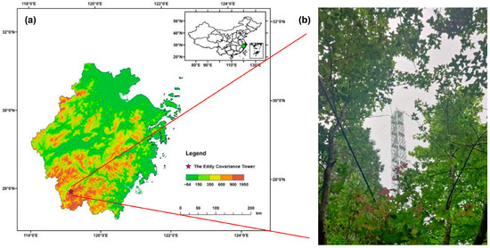
Figure 1.
(a) Geographical map of the study area and (b) the eddy covariance tower.
The flux tower is set up at an altitude of 1350 m in Fengyang Mountain (119°10′15″ E, 27°54′22″ N). The dominant vegetation type is coniferous and broad-leaved mixed forest, representing about 80% of the study area’s total land area. The average canopy height is around 15 m, and the average forest age is approximately 40 years. The constructive species include Schima superba, Cunninghamia lanceolata, Castanopsis eyrei, and Cyclobalanopsis multinervis, among others. The soil type is acidic yellow-brown soil, with a pH of approximately 4.245 ± 0.094 [22], and the soil density is approximately 0.940 ± 0.016 g cm−3 [23].
2.2. Data Collection and Processing
An open-circuit eddy flux observation system with a height of 40 m (27°54′22″ N, 119°10′15″ E) was built in the center of the study area. This system comprises three major components: a flux system, a gradient system, and a profiling system. The flux system is installed at a height of 40 m on the flux tower and equipped with primary sensors, including a three-dimensional ultrasound and CO2/H2O analyzer (IRGASON, Campbell Scientific Inc., Logan, UT, USA), a four-component radiation meter (CNR4, Kipp & Zonen, Delft, Netherlands), an air temperature and humidity sensor (HMP155A, Vaisala, Helsinki, Finland), and a soil heat flux plate (HFP01, Hukseflux, Delft, Netherlands). The six-layer gradient system is capable of measuring meteorological variables at different spatial heights (2, 8, 16, 24, 32, and 40 m) and soil depths (10, 20, 30, 40, 60, and 90 cm), utilizing sensors such as soil temperature sensors (TCAV, Campbell Scientific Inc., Logan, UT, USA), soil moisture sensors (CS616, Campbell Scientific Inc., Logan, UT, USA), wind direction sensors (020C, Met One Instruments Inc., OR, USA), wind speed sensors (010C, Met One Instruments Inc., OR, USA), a rain gauge (RG3-M, Oneset, MA, USA), and air temperature and humidity sensors (HMP155A, Campbell Scientific Inc., Logan, UT, USA). The profiling system, primarily composed of Atmospheric Profile 200 (AP200, Campbell Scientific Inc., Logan, UT, USA) and air intake components, measures the concentrations of CO2 and H2O in the air at six observation levels (spatial heights of 2, 8, 16, 24, 32, and 40 m).
Figure 2 shows a brief process of flux data processing. The raw data collected by the ultrasonic anemometer and the infrared gas analyzer at a frequency of 10 Hz within the eddy flux observation system were processed through an online program (EasyFlux™-PC, Campbell Scientific Instruments, USA, https://www.campbellsci.com/easyflux-pc [accessed on 10 May 2023]) to yield data with a time step of 30 min. The processing techniques employed include, but are not limited to, plane fitting, Webb, Pearman, and Leuning (WPL) correction, friction wind speed filtering, and outlier removal. To ensure the quality of the data, abnormal half-hour flux data were further discarded based on the following criteria: (1) data when the carbon flux exceeds the typical threshold for forest ecosystem carbon fluxes; (2) data indicating sensor malfunctions, such as signal anomalies; (3) data collected within an hour before or after a rainfall event; (4) data when the vertical wind speed falls below the seasonal threshold. For a detailed account of flux calculation and correction methods, refer to Wutzler et al. [24]. The concurrent gradient meteorological observation system recorded meteorological variables in 30 min intervals, including air temperature (Tair), air relative humidity (RH), soil temperature (Tsoil), soil moisture (SWC), precipitation (PRCP), saturated vapor pressure difference (VPD), and solar radiation (Rg).
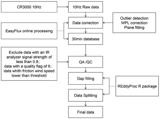
Figure 2.
Brief flowchart of data flow.
2.3. Data Calculation
2.3.1. Calculation of Evapotranspiration (ET)
The calculation formula of evapotranspiration ET is as follows [25,26]:
where LE is the latent heat flux (W m−2), (597 − 0.564T) is the vaporization heat of water (cal g−1), 0.43 is the unit conversion coefficient, T is the air temperature at the canopy height, the evapotranspiration (ET) is obtained by adding the data of each 0.5 h in a day, and the unit of the result is in mm.
2.3.2. Calculation of Gross Primary Productivity (GPP)
First, the net ecosystem exchange of CO2 (NEE) is calculated based on the method proposed by Zhang Mi et al. [27].
The vertical turbulent flux of CO2 at the measurement height zr can be expressed as:
where represents the fluctuation in vertical wind speed, represents the fluctuation in CO2 density, and the overline indicates the average over a certain time interval.
The CO2 storage flux below the observation height of the eddy covariance system is calculated using the CO2 concentration profile method:
where Fs represents the CO2 storage flux (mg CO2 m−2 s−1) below the observation flux height of 40 m; z represents the observation heights of the profile method (2, 8, 16, 24, 32, and 40 m); represents the average CO2 concentration between the observation platforms; and represents the measurement time interval.
NEE is defined as the sum of the vertical turbulent flux of CO2 (Fc) and the CO2 storage flux (Fs) below the observation height. Mathematically, this can be expressed as
The “REddyProc” package in RStudio provides functions and algorithms to partition NEE into ecosystem respiration (Re) and GPP based on various methods, such as nighttime flux partitioning, light response curves, and temperature response curves. Using the “REddyProc” package in RStudio (https://CRAN.R-project.org/package=REddyProc/, accessed on 10 May 2023), the calculated NEE data can be partitioned into Re and GPP [24]. The relationship between these three components is
2.3.3. Calculation of WUE
Here, we calculated ecosystem WUE as the ratio of gross primary productivity (GPP) to evapotranspiration (ET) using the following formula:
where WUE is ecosystem water use efficiency (gC kg−1 H2O), GPP is ecosystem total primary productivity (gC m−2), and ET is ecosystem evapotranspiration (mm).
2.4. Ridge Regression Analysis
To minimize the impact of multicollinearity on identifying the correct factors influencing the variability in WUE, we conducted ridge regression analysis to assess the effects of various meteorological factors on WUE across different time scales. Ridge regression is a type of linear regularized and biased estimation regression method, fundamentally an enhanced version of the least squares estimation method [28].
3. Results
3.1. Environmental Condition
Table 1 shows the maximum, minimum, and average values of various environmental variables during the monitoring period. The trend of the monthly mean or cumulative value of all climatic variables over time during the study period is shown in Figure 3. Temperature, solar radiation, and air relative humidity peaked in July and gradually declined thereafter. The precipitation in the study area is abundant and shows obvious seasonal changes. The average annual precipitation is 1875 mm, and the precipitation from March to August accounts for 73.59% of the total annual precipitation (Figure 3e). June is the wettest month of the year, with a monthly average of 401 mm. The soil moisture content was strongly correlated with rainfall and reached a maximum of 20.94% in June (Figure 3f).

Table 1.
The monthly maximum, minimum, and average values of environmental variables.
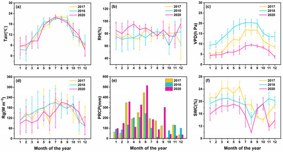
Figure 3.
Variation characteristics of monthly mean or cumulative values of environmental factors calculated using 2017, 2018, and 2020 data. (a) Tair, (b) RH, (c) VPD, (d) Rg, (e) PRCP, and (f) SWC. The values in the line chart represent the monthly mean values (means ±1 SE), and the values in the histogram represent the monthly cumulative values.
3.2. The Variation Characteristics of WUE at Multiple Time Scales
The WUE of coniferous and broad-leaved mixed forest ecosystems had obvious diurnal variation characteristics (Figure 4a). During the study period, the mean WUE of the ecosystem was 6.12 gC kg−1 H2O, and the WUE of the ecosystem varied greatly over time, ranging from 4.84 gC kg−1 H2O to 7.88 gC kg−1 H2O. Although it fluctuated within a certain range, the average daily variation in WUE in 2017, 2018, and 2020 basically showed a gradual increase from 7:00 to 14:30 and reached a peak (6.75 gC kg−1 H2O, 7.88 gC kg−1 H2O, 7.48 gC kg−1 H2O), then gradually decreased. During the study period, the WUE (2.92 gC kg−1 H2O) in the growing season (May–October) was slightly higher than that in the non-growing season (November–April) (2.64 gC kg−1 H2O). Minimum WUE occurred in July 2018 (1.15 gC kg−1 H2O), and the maximum occurred in September 2018 (4.31 gC kg−1 H2O). At the seasonal scale, the mean WUE in autumn and winter (2.97 gC kg−1 H2O) was higher than that in spring and summer (2.59 gC kg−1 H2O).
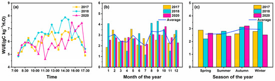
Figure 4.
Dynamic characteristics of WUE under multiple time scales. (a) Half-hour scale, (b) monthly scale, and (c) seasonal scale. The line in (b) represents the monthly average of three years, and the line in (c) represents the seasonal average of three years.
We found that there were differences in ecosystem WUE among different site years (Figure 4). WUE in 2018 was significantly higher than that in 2017 and 2020, which may be related to the low precipitation in 2018. According to the site precipitation observation, 2018 was a drier year in the study area compared with the average site precipitation in 2017 and 2020. The total precipitation in 2018 was 1379 mm, which was 31.47% and 38.27% lower than that in 2017 (201 mm) and 2020 (223 mm), respectively. The annual precipitation in 2018 was one standard deviation lower than the observed multi-year average precipitation (170 mm) from 1979 to 2016 in the study area (Figure 5).
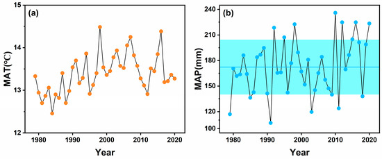
Figure 5.
(a) Temporal changes in mean annual temperature (MAT) and (b) mean annual precipitation (MAP) at Fengyang mountain meteorological station during 1979–2020. Shaded area in (b) indicates ± 1 standard deviation in MAP during 1979–2020.
The soil moisture data were collected from sensors positioned at a depth of 10 cm, representing the volumetric water content of the topsoil. Despite 2018 being characterized as a drought year, the soil moisture levels in 2018 did not significantly differ from those of 2017 and 2020. Prior research [29,30] has shown that the uneven spatial and temporal distribution of rainfall directly impacts the variability and dynamics of soil moisture. Specifically, evenly distributed rainfall favors the accumulation and retention of soil moisture, whereas concentrated or intermittent rainfall may result in water loss or surface runoff. Additionally, the intensity of rainfall determines the rate and depth of water infiltration into the soil [31]. High-intensity rainfall can cause rapid water loss, whereas low-intensity rainfall promotes gradual infiltration into deeper soil layers. Integrating the monthly rainfall data for each year (Figure 3e), it is evident that the more uniform rainfall pattern in 2018 mitigated the effects of drought on soil moisture, resulting in moderate soil moisture levels in 2018 compared to 2017 and 2020.
3.3. Driving Factors of WUE Change at Different Time Scales
To identify potential dominant factors contributing to the variability in WUE, we calculated Pearson’s correlations between WUE and each environmental factor (Figure 6). On the half-hour scale (Figure 6a1), we observed that WUE was significantly positively correlated with air temperature (Tair) (r = 0.77, p < 0.01), VPD (r = 0.78, p < 0.01), and solar radiation (Rg) (r = 0.45, p < 0.05) and negatively correlated with RH (r = −0.74, p < 0.01). No significant correlation was found between WUE and SWC (r = −0.34, p > 0.05). At the monthly scale, we did not observe a significant correlation between WUE and the meteorological factors (Figure 6b1). Ecosystem WUE at the seasonal scale was only significantly negatively correlated with precipitation (r = −0.99, p < 0.05). Additionally, we analyzed the Pearson correlation between meteorological factors at different time scales (Figure 6a2–c2). The results indicated a significant linear correlation between meteorological factors, especially between VPD and Rg. Although this correlation weakened with the extension of the time scale, the presence of correlation between explanatory variables often implies multicollinearity issues. In factor analysis, variables exhibiting multicollinearity may lead to instability in factor loading, affecting the outcomes of the factor analysis and rendering the parameter estimation of the regression model uninterpretable.
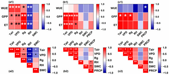
Figure 6.
Pearson correlation between WUE, GPP, ET, and environmental factors at different time scales and the correlation between environmental factors at different time scales. (a1–c1) Pearson correlation between WUE and meteorological factors at the half-hour scale, monthly scale, and seasonal scale, respectively. (a2–c2) Pearson correlation between meteorological factors at half-hour scale, monthly scale, and seasonal scale, respectively. Stars in the box indicate statistically significant differences, * represents p < 0.05, and ** represents p < 0.01.
Based on the ridge regression analysis of the average WUE of the ecosystem and meteorological factors (Figure 7), significant differences were observed in the driving factors that dominated WUE variation across different time scales. At the half-hour scale, WUE exhibited a significant positive correlation with Tair (R.C. = 0.30, p < 0.01) and VPD (R.C. = 0.19, p < 0.05) and a significant negative correlation with RH (R.C. = −0.08, p < 0.05). Rg and SWC did not significantly affect WUE. Together, Tair and VPD accounted for 48.39% of the variation in ecosystem WUE. At the monthly scale, WUE was significantly negatively correlated with Tair (R.C. = −0.26, p < 0.05), RH (R.C. = −0.24, p < 0.05), and PRCP (R.C. = −0.24, p < 0.05), whereas VPD, Rg, and SWC showed no significant effect on WUE. By the seasonal scale, none of the relationships between ecosystem WUE and the meteorological factors were significant.
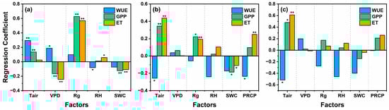
Figure 7.
The independent effects of environmental factors on WUE, ET, and GPP were obtained by ridge regression at (a) half-hour scale, (b) monthly scale, and (c) seasonal scale. Stars over the bar indicate statistically significant differences, * represents p < 0.05, and ** represents p < 0.01.
3.4. Response of WUE Components to Environmental Changes
Through Pearson correlation analysis, it was discovered that at the half-hour scale, several major meteorological factors influencing ecosystem WUE, such as Tair, VPD, Rg, and RH, also significantly impact GPP and ET in the same direction. Though the correlation between meteorological factors and WUE disappeared at the monthly scale (Figure 6c1), a significant positive correlation between Tair, VPD, and Rg with GPP and ET persisted. This positive correlation between GPP and Tair, VPD, and Rg remained significant even when extended to the seasonal scale, although the correlation between ET and various meteorological factors became less apparent.
Coupling these findings with the results from ridge regression analysis revealed that meteorological factors often influence GPP and ET in the same direction; that is, an increase in a meteorological factor such as Tair or VPD corresponds with an increase or decrease in both GPP and ET. Normally, when a meteorological factor affects GPP and ET oppositely, its effect on WUE is more straightforward to discern. However, when a meteorological factor has a similar effect on both GPP and ET, determining its independent impact on GPP and ET becomes crucial for understanding its influence on ecosystem WUE. Ridge regression analysis effectively addresses this issue.
We found VPD to be significantly negatively correlated with GPP (R.C. = −0.17, p < 0.01) and ET (R.C. = −0.24, p < 0.01) on a half-hourly scale (Figure 7a), yet it was significantly positively correlated with WUE (R.C. = 0.18, p < 0.05). This pattern emerges because elevated VPD leads to more variation in ET compared to GPP variation, resulting in a greater decrease in ET. Consequently, WUE increases with an increase in VPD (R.C. = 0.18, p < 0.05). Conversely, when Rg increased at the half-hour scale, GPP (R.C. = 0.63, p < 0.01) was significantly positively correlated with ET (R.C. = 0.56, p < 0.01). In this scenario, elevated Rg causes more GPP variation compared to ET variation, leading to a significant increase in GPP. Thus, the result is an increase in WUE due to the rise in Rg. The fluctuation in WUE reflects the process of the coupled changes of carbon and water in the ecosystem. These results demonstrate that VPD is more closely related to the water cycle process, whereas Rg is more intimately connected with the carbon cycle process on a short time scale.
4. Discussion
4.1. WUE Responds Differently to Changes in Environmental Factors at Different Time Scales
Our results suggest that WUE exhibits different temporal variation characteristics at various scales, and the dominant environmental factors influencing ecosystem WUE also shift over time. This finding is consistent with previous research [32,33,34,35,36]. At shorter time scales, ecosystem WUE is more likely to respond to changes in environmental factors because its components, namely, GPP and ET, are more sensitive to environmental changes within a half-hour or shorter time scale [16,37,38]. Conversely, the response of ecosystem WUE to changes in environmental factors is less apparent over longer time scales. This observation might be attributed to our study’s focus solely on the impact of environmental factors on WUE. We hypothesize that physiological and ecological factors of vegetation, such as leaf area index, atmospheric CO2 concentration, and intercellular CO2 concentration, may be key drivers of WUE over extended periods [39,40].
Previous results have indicated that an increase in VPD leads to higher GPP and ET over short time scales, while often resulting in decreased WUE [10,28,41]. However, our findings reveal a significant negative correlation between VPD and both GPP and ET in the mixed coniferous and broad-leaved forest ecosystem. Due to the asymmetrical response of GPP and ET to changes in VPD, WUE increased as VPD rose. It is widely acknowledged that VPD levels are directly associated with atmospheric water demand, influencing surface water conduction and evapotranspiration. VPD can significantly restrict evapotranspiration in biomes by modifying stomatal behavior in plants [42,43]. Some researchers have identified an optimal VPD range for plant growth between 8.0 and 9.5 h Pa [44]. Our observations show the mean VPD in the study area was 11.04 hPa, surpassing the ideal range for plant growth. Under such conditions, plants may actively close their stomata to mitigate water stress induced by high VPD, thereby reducing water loss and preventing critical water tension in the xylem [45]. This adaptation often comes at the cost of reduced photosynthesis. Although plant transpiration rates may initially increase with rising VPD, they tend to decrease after surpassing a certain threshold [46]. Thus, we speculate the observed decrease in GPP and ET with increasing VPD in this ecosystem could be attributed to the elevated VPD levels. The impact of VPD on WUE and its components was significant only at the half-hour scale, but not on monthly or seasonal scales. This discrepancy is likely because the response of stomatal conductance to VPD fluctuations and the corresponding adjustments in photosynthesis and transpiration can occur within minutes to hours, rendering the effects of VPD changes on ecosystem WUE negligible at broader time scales.
4.2. The Main Drivers of WUE Variation in Ecosystems
Unlike the least squares method, ridge regression forgoes unbiasedness. It incorporates a penalty term into the cost function, penalizing larger parameter values when the independent variables are highly correlated. This approach ensures that the estimated partial regression coefficients are more aligned with the actual scenario, thus enhancing the stability and reliability of the regression model. Consequently, ridge regression is particularly well suited for analyses involving significant multicollinearity among independent variables [28]. Furthermore, in the results of ridge regression, the regression coefficients of various environmental factors and WUE indicate their independent effects on the variation in WUE. By comparing the magnitudes of the ridge regression coefficients, we can identify the main drivers of WUE.
In the optimum interval, the plant photosynthetic rate increases with temperature [41,47]. Our results indicate that temperature, as a crucial factor in determining plant photosynthetic rate and transpiration, positively affects GPP and ET across all time scales. Compared to other environmental factors, temperature offers the most substantial explanation for the variation in ecosystem WUE at all observed scales (half-hour scale R.C. = 0.30; monthly scale R.C. = −0.26; seasonal scale R.C. = 0.51). These findings underscore temperature as the most significant environmental factor driving WUE variations in the coniferous and broad-leaved mixed forest ecosystem, aligning with prior research [48,49,50].
We also observed a significant negative impact of RH on ecosystem WUE at both the half-hour and monthly scales. Though the intensity of this negative correlation diminished at the seasonal scale, RH still plays a role in explaining WUE variation. Previous studies have indicated that relative humidity and vapor pressure deficit predominantly influence actual and potential evapotranspiration. The air’s relative humidity to some extent determines the sensitivity of transpiration to stomatal conductance [51], with an increase in relative humidity facilitating plant water transpiration [52,53,54,55]. Our study corroborates this perspective, demonstrating that WUE decreases with rising RH.
5. Conclusions
Here, we used eddy covariance tower observations to quantify the GPP, ET, and WUE of the coniferous and broad-leaved mixed forest ecosystem in East China in 2017, 2018, and 2020, and we analyzed the environmental factors driving WUE changes at multiple time scales. We found that WUE exhibited different characteristics of changes at various time scales and variations in response to environmental factors. Specifically, at the half-hour scale, the ecosystem WUE was sensitive to changes in all environmental factors. Temperature, relative humidity, and precipitation emerged as the three major factors that dominated WUE changes at the monthly scale. At the seasonal scale, temperature could explain 51% of the variation in WUE (R.C. = −0.51, p < 0.05), and other meteorological factors had no significant effect on WUE. Our findings underscore the varying effects of environmental factors on WUE variation across different time scales. Moreover, vegetation physiological and ecological factors should be considered to better understand the response of ecosystem WUE to climate change.
Author Contributions
Data acquisition, S.D. and D.X.; methodology, J.J.; software, S.D. and D.X.; investigation, S.D. and S.L.; resources, J.J.; data analysis, S.D. and L.L.; writing—original draft preparation, S.D.; writing—review and editing, J.J.; visualization, S.D. and D.X.; project administration, J.J.; funding acquisition, J.J. All authors have read and agreed to the published version of the manuscript.
Funding
This research was funded by the Scientific Research Project of Baishanzu National Park, grant numbers 2022JBGS03 and 2021ZDLY01, and the Postgraduate Research and Practice Innovation Program of Jiangsu Province grant number SJCX23_0342.
Data Availability Statement
The data presented in this study are available on request from the corresponding author.
Acknowledgments
We are grateful for the assistance of Xingchang Wang of Northeast Forestry University in data processing. We thank Bai Yang for help in data acquisition and processing.
Conflicts of Interest
The authors declare no conflicts of interest.
References
- Bertolino, L.T.; Caine, R.S.; Gray, J.E. Impact of Stomatal Density and Morphology on Water-Use Efficiency in a Changing World. Front. Plant Sci. 2019, 10, 225. [Google Scholar] [CrossRef]
- López-Calcagno, P.E.; Brown, K.L.; Simkin, A.J.; Fisk, S.J.; Vialet-Chabrand, S.; Lawson, T.; Raines, C.A. Stimulating Photosynthetic Processes Increases Productivity and Water-Use Efficiency in the Field. Nat. Plants 2020, 6, 1054–1063. [Google Scholar] [CrossRef]
- Li, F.; Xiao, J.; Chen, J.; Ballantyne, A.; Jin, K.; Li, B.; Abraha, M.; John, R. Global Water Use Efficiency Saturation Due to Increased Vapor Pressure Deficit. Science 2023, 381, 672–677. [Google Scholar] [CrossRef] [PubMed]
- Zhang, Z.; Zhang, L.; Xu, H.; Creed, I.F.; Blanco, J.A.; Wei, X.; Sun, G.; Asbjornsen, H.; Bishop, K. Forest Water-Use Efficiency: Effects of Climate Change and Management on the Coupling of Carbon and Water Processes. For. Ecol. Manag. 2023, 534, 120853. [Google Scholar] [CrossRef]
- Hu, Z.; Yu, G.; Wang, Q.; Zhao, F. Research Progress on Ecosystem Water Use Efficiency. Acta Ecol. Sin. 2009, 29, 1498–1507. [Google Scholar]
- Huang, M.; Piao, S.; Sun, Y.; Ciais, P.; Cheng, L.; Mao, J.; Poulter, B.; Shi, X.; Zeng, Z.; Wang, Y. Change in Terrestrial Ecosystem Water-Use Efficiency over the Last Three Decades. Glob. Change Biol. 2015, 21, 2366–2378. [Google Scholar] [CrossRef] [PubMed]
- Hatfield, J.L.; Dold, C. Water-Use Efficiency: Advances and Challenges in a Changing Climate. Front. Plant Sci. 2019, 10, 103. [Google Scholar] [CrossRef]
- Niu, S.; Xing, X.; Zhang, Z.; Xia, J.; Zhou, X.; Song, B.; Li, L.; Wan, S. Water-Use Efficiency in Response to Climate Change: From Leaf to Ecosystem in a Temperate Steppe. Glob. Chang. Biol. 2011, 17, 1073–1082. [Google Scholar] [CrossRef]
- Wu, X.; Li, X.; Chen, Y.; Bai, Y.; Tong, Y.; Wang, P.; Liu, H.; Wang, M.; Shi, F.; Zhang, C.; et al. Atmospheric Water Demand Dominates Daily Variations in Water Use Efficiency in Alpine Meadows, Northeastern Tibetan Plateau. JGR Biogeosci. 2019, 124, 2174–2185. [Google Scholar] [CrossRef]
- Peddinti, S.R.; Kambhammettu, B.V.N.P.; Rodda, S.R.; Thumaty, K.C.; Suradhaniwar, S. Dynamics of Ecosystem Water Use Efficiency in Citrus Orchards of Central India Using Eddy Covariance and Landsat Measurements. Ecosystems 2020, 23, 511–528. [Google Scholar] [CrossRef]
- Wang, T.; Tang, X.; Zheng, C.; Gu, Q.; Wei, J.; Ma, M. Differences in Ecosystem Water-Use Efficiency among the Typical Croplands. Agric. Water Manag. 2018, 209, 142–150. [Google Scholar] [CrossRef]
- Wei, S.; Chu, X.; Sun, B.; Yuan, W.; Song, W.; Zhao, M.; Wang, X.; Li, P.; Han, G. Climate Warming Negatively Affects Plant Water-Use Efficiency in a Seasonal Hydroperiod Wetland. Water Res. 2023, 242, 120246. [Google Scholar] [CrossRef]
- Xiao, J.; Sun, G.; Chen, J.; Chen, H.; Chen, S.; Dong, G.; Gao, S.; Guo, H.; Guo, J.; Han, S.; et al. Carbon Fluxes, Evapotranspiration, and Water Use Efficiency of Terrestrial Ecosystems in China. Agric. For. Meteorol. 2013, 182–183, 76–90. [Google Scholar] [CrossRef]
- Wang, M.; Chen, Y.; Wu, X.; Bai, Y. Forest-Type-Dependent Water Use Efficiency Trends Across the Northern Hemisphere. Geophys. Res. Lett. 2018, 45, 8283–8293. [Google Scholar] [CrossRef]
- Mathias, J.M. Tree Growth and Water Use Efficiency during the Twentieth Century: From Global Trends to Local Drivers. Ph.D. Thesis, West Virginia University Libraries, Morgantown, WV, USA, 2020. [Google Scholar]
- Liu, Z.; Ji, X.; Ye, L.; Jiang, J. Inherent Water-Use Efficiency of Different Forest Ecosystems and Its Relations to Climatic Variables. Forests 2022, 13, 775. [Google Scholar] [CrossRef]
- Wolf, A.; Anderegg, W.R.L.; Pacala, S.W. Optimal Stomatal Behavior with Competition for Water and Risk of Hydraulic Impairment. Proc. Natl. Acad. Sci. USA 2016, 113, E7222–E7230. [Google Scholar] [CrossRef]
- Chen, C.; Riley, W.J.; Prentice, I.C.; Keenan, T.F. CO2 Fertilization of Terrestrial Photosynthesis Inferred from Site to Global Scales. Proc. Natl. Acad. Sci. USA 2022, 119, e2115627119. [Google Scholar] [CrossRef]
- Liang, X.; Wang, D.; Ye, Q.; Zhang, J.; Liu, M.; Liu, H.; Yu, K.; Wang, Y.; Hou, E.; Zhong, B.; et al. Stomatal Responses of Terrestrial Plants to Global Change. Nat. Commun. 2023, 14, 2188. [Google Scholar] [CrossRef]
- Tan, Z.; Zhang, Y.; Deng, X.; Song, Q.; Liu, W.; Deng, Y.; Tang, J.; Liao, Z.; Zhao, J.; Song, L.; et al. Interannual and Seasonal Variability of Water Use Efficiency in a Tropical Rainforest: Results from a 9 Year Eddy Flux Time Series. JGR Atmos. 2015, 120, 464–479. [Google Scholar] [CrossRef]
- Adams, M.A.; Buckley, T.N.; Turnbull, T.L. Rainfall Drives Variation in Rates of Change in Intrinsic Water Use Efficiency of Tropical Forests. Nat. Commun. 2019, 10, 3661. [Google Scholar] [CrossRef]
- Zhao, Y.; Meng, M.; Zhang, J.; Ma, J.; Liu, S. A Study on Soil Aggregates and Their Stability in the Main Forest Types of Fengyang Mountain. J. Nanjing For. Univ. 2018, 42, 84–90. [Google Scholar]
- Chen, M.; Zhao, Y.; Zhang, J.; Wang, H.; Meng, M.; Liu, X.; Li, C.; Xie, D. Characteristics of Soil Organic Carbon in Typical Forest Types of Fengyang Mountain. J. Northeast For. Univ. 2022, 50, 69–75. [Google Scholar] [CrossRef]
- Wutzler, T.; Lucas-Moffat, A.; Migliavacca, M.; Knauer, J.; Sickel, K.; Šigut, L.; Menzer, O.; Reichstein, M. Basic and Extensible Post-Processing of Eddy Covariance Flux Data with REddyProc. Biogeosciences 2018, 15, 5015–5030. [Google Scholar] [CrossRef]
- Niu, X. Study on Carbon and Water Fluxes and Water Use Efficiency of Sharp-Toothed Oak Forest Ecosystem in the Warm Temperate Zone. Ph.D. Thesis, Chinese Academy of Forestry, Beijing, China, 2022. [Google Scholar]
- Liu, C.; Zhang, Z.; Sun, G.; Zha, T.; Zhu, J.; Shen, H.; Chen, J.; Fang, X.; Chen, J. Evaluation of Evapotranspiration and Its Environmental Response in Poplar Plantation Ecosystems Based on Eddy Covariance Technique and Stem Sap Flow Method. J. Plant Ecol. 2009, 33, 706–718. [Google Scholar]
- Zhang, M.; Wen, X.-F.; Yu, G.-R.; Zhang, L.-M.; Fu, Y.-L.; Sun, X.-M.; Han, S.-J. Effects of CO2 Storage Flux on Carbon Budget of Forest Ecosystem. Chin. J. Appl. Ecol. 2010, 21, 1201. [Google Scholar]
- Guerrieri, R.; Belmecheri, S.; Ollinger, S.V.; Asbjornsen, H.; Jennings, K.; Xiao, J.; Stocker, B.D.; Martin, M.; Hollinger, D.Y.; Bracho-Garrillo, R.; et al. Disentangling the Role of Photosynthesis and Stomatal Conductance on Rising Forest Water-Use Efficiency. Proc. Natl. Acad. Sci. USA 2019, 116, 16909–16914. [Google Scholar] [CrossRef] [PubMed]
- Singh, N.K.; Emanuel, R.E.; McGlynn, B.L.; Miniat, C.F. Soil Moisture Responses to Rainfall: Implications for Runoff Generation. Water Resour. Res. 2021, 57, e2020WR028827. [Google Scholar] [CrossRef]
- Liu, Y.; Yang, Y. Spatial-Temporal Variability Pattern of Multi-Depth Soil Moisture Jointly Driven by Climatic and Human Factors in China. J. Hydrol. 2023, 619, 129313. [Google Scholar] [CrossRef]
- Zhang, P.; Xiao, P.; Yao, W.; Liu, G.; Sun, W. Profile Distribution of Soil Moisture Response to Precipitation on the Pisha Sandstone Hillslopes of China. Sci. Rep. 2020, 10, 9136. [Google Scholar] [CrossRef]
- Tong, X.; Zhang, J.; Meng, P.; Li, J.; Zheng, N. Ecosystem Water Use Efficiency in a Warm-Temperate Mixed Plantation in the North China. J. Hydrol. 2014, 512, 221–228. [Google Scholar] [CrossRef]
- Song, Q.-H.; Fei, X.-H.; Zhang, Y.-P.; Sha, L.-Q.; Liu, Y.-T.; Zhou, W.-J.; Wu, C.-S.; Lu, Z.-Y.; Luo, K.; Gao, J.-B.; et al. Water Use Efficiency in a Primary Subtropical Evergreen Forest in Southwest China. Sci. Rep. 2017, 7, 43031. [Google Scholar] [CrossRef] [PubMed]
- Aguilos, M.; Stahl, C.; Burban, B.; Hérault, B.; Courtois, E.; Coste, S.; Wagner, F.; Ziegler, C.; Takagi, K.; Bonal, D. Interannual and Seasonal Variations in Ecosystem Transpiration and Water Use Efficiency in a Tropical Rainforest. Forests 2018, 10, 14. [Google Scholar] [CrossRef]
- Guo, F.; Jin, J.; Yong, B.; Wang, Y.; Jiang, H. Responses of Water Use Efficiency to Phenology in Typical Subtropical Forest Ecosystems—A Case Study in Zhejiang Province. Sci. China Earth Sci. 2020, 63, 145–156. [Google Scholar] [CrossRef]
- An, X. Responses of Water Use Efficiency to Climate Change in Evapotranspiration and Transpiration Ecosystems. Ecol. Indic. 2022, 141, 109157. [Google Scholar] [CrossRef]
- Gentine, P.; Green, J.K.; Guérin, M.; Humphrey, V.; Seneviratne, S.I.; Zhang, Y.; Zhou, S. Coupling between the Terrestrial Carbon and Water Cycles—A Review. Environ. Res. Lett. 2019, 14, 083003. [Google Scholar] [CrossRef]
- Zhang, L.; Xiao, J.; Zheng, Y.; Li, S.; Zhou, Y. Increased Carbon Uptake and Water Use Efficiency in Global Semi-Arid Ecosystems. Environ. Res. Lett. 2020, 15, 034022. [Google Scholar] [CrossRef]
- Desai, A.R.; Murphy, B.A.; Wiesner, S.; Thom, J.; Butterworth, B.J.; Koupaei-Abyazani, N.; Muttaqin, A.; Paleri, S.; Talib, A.; Turner, J.; et al. Drivers of Decadal Carbon Fluxes Across Temperate Ecosystems. JGR Biogeosci. 2022, 127, e2022JG007014. [Google Scholar] [CrossRef] [PubMed]
- Launiainen, S.; Katul, G.G.; Leppä, K.; Kolari, P.; Aslan, T.; Grönholm, T.; Korhonen, L.; Mammarella, I.; Vesala, T. Does Growing Atmospheric CO 2 Explain Increasing Carbon Sink in a Boreal Coniferous Forest? Glob. Chang. Biol. 2022, 28, 2910–2929. [Google Scholar] [CrossRef] [PubMed]
- Li, S.; Agathokleous, E.; Li, S.; Xu, Y.; Xia, J.; Feng, Z. Climate Gradient and Leaf Carbon Investment Influence the Effects of Climate Change on Water Use Efficiency of Forests: A Meta-analysis. Plant Cell Environ. 2024, 47, 1070–1083. [Google Scholar] [CrossRef]
- Fletcher, A.L.; Sinclair, T.R.; Allen, L.H. Transpiration Responses to Vapor Pressure Deficit in Well Watered ‘Slow-Wilting’ and Commercial Soybean. Environ. Exp. Bot. 2007, 61, 145–151. [Google Scholar] [CrossRef]
- Novick, K.A.; Ficklin, D.L.; Stoy, P.C.; Williams, C.A.; Bohrer, G.; Oishi, A.C.; Papuga, S.A.; Blanken, P.D.; Noormets, A.; Sulman, B.N.; et al. The Increasing Importance of Atmospheric Demand for Ecosystem Water and Carbon Fluxes. Nat. Clim. Chang. 2016, 6, 1023–1027. [Google Scholar] [CrossRef]
- Li, J. Response of Stomatal Conductance and Plant Hormones of Several Plant Leaves to Atmospheric Humidity. Ph.D. Thesis, Shandong University, Jinan, China, 2014. [Google Scholar]
- Running, S.W. Environmental Control of Leaf Water Conductance in Conifers. Can. J. For. Res. 1976, 6, 104–112. [Google Scholar] [CrossRef]
- Franks, P.J.; Cowan, I.R.; Farquhar, G.D. The Apparent Feedforward Response of Stomata to Air Vapour Pressure Deficit: Information Revealed by Different Experimental Procedures with Two Rainforest Trees. Plant Cell Environ. 1997, 20, 142–145. [Google Scholar] [CrossRef]
- Wang, D.; Wang, H.; Wang, P.; Ling, T.; Tao, W.; Yang, Z. Warming Treatment Methodology Affected the Response of Plant Ecophysiological Traits to Temperature Increases: A Quantitive Meta-Analysis. Front. Plant Sci. 2019, 10, 957. [Google Scholar] [CrossRef] [PubMed]
- Zhang, Z.; Jiang, H.; Liu, J.X.; Zhou, G.M.; Liu, S.R.; Zhang, X.Y. Assessment on Water Use Efficiency under Climate Change and Heterogeneous Carbon Dioxide in China Terrestrial Ecosystems. Procedia Environ. Sci. 2012, 13, 2031–2044. [Google Scholar] [CrossRef]
- Tang, X.; Li, H.; Desai, A.R.; Nagy, Z.; Luo, J.; Kolb, T.E.; Olioso, A.; Xu, X.; Yao, L.; Kutsch, W.; et al. How Is Water-Use Efficiency of Terrestrial Ecosystems Distributed and Changing on Earth? Sci. Rep. 2014, 4, 7483. [Google Scholar] [CrossRef] [PubMed]
- Sun, Y.; Piao, S.; Huang, M.; Ciais, P.; Zeng, Z.; Cheng, L.; Li, X.; Zhang, X.; Mao, J.; Peng, S.; et al. Global Patterns and Climate Drivers of Water-use Efficiency in Terrestrial Ecosystems Deduced from Satellite-based Datasets and Carbon Cycle Models. Glob. Ecol. Biogeogr. 2016, 25, 311–323. [Google Scholar] [CrossRef]
- Pan, S.; Chen, G.; Ren, W.; Dangal, S.R.S.; Banger, K.; Yang, J.; Tao, B.; Tian, H. Responses of Global Terrestrial Water Use Efficiency to Climate Change and Rising Atmospheric CO2 Concentration in the Twenty-First Century. Int. J. Digit. Earth 2018, 11, 558–582. [Google Scholar] [CrossRef]
- Shenbin, C.; Yunfeng, L.; Thomas, A. Climatic Change on the Tibetan Plateau: Potential Evapotranspiration Trends from 1961–2000. Clim. Chang. 2006, 76, 291–319. [Google Scholar] [CrossRef]
- Zhang, T.; Zhang, Y.; Xu, M.; Zhu, J.; Chen, N.; Jiang, Y.; Huang, K.; Zu, J.; Liu, Y.; Yu, G. Water Availability Is More Important than Temperature in Driving the Carbon Fluxes of an Alpine Meadow on the Tibetan Plateau. Agric. For. Meteorol. 2018, 256–257, 22–31. [Google Scholar] [CrossRef]
- Tang, Y.-Y.; Chen, J.-P.; Zhang, F.; Yuan, S.-S. Spatiotemporal Analysis of Evapotranspiration and Effects of Water and Heat on Water Use Efficiency. Water 2021, 13, 3019. [Google Scholar] [CrossRef]
- Li, Y.; Zhang, K.; Liu, L. Water Use Efficiency at Multi-Time Scales and Its Response to Episodic Drought and Wet Periods in a Typical Subtropical Evergreen Forest of Southeast China. Ecol. Indic. 2023, 151, 110254. [Google Scholar] [CrossRef]
Disclaimer/Publisher’s Note: The statements, opinions and data contained in all publications are solely those of the individual author(s) and contributor(s) and not of MDPI and/or the editor(s). MDPI and/or the editor(s) disclaim responsibility for any injury to people or property resulting from any ideas, methods, instructions or products referred to in the content. |
© 2024 by the authors. Licensee MDPI, Basel, Switzerland. This article is an open access article distributed under the terms and conditions of the Creative Commons Attribution (CC BY) license (https://creativecommons.org/licenses/by/4.0/).