Article

Unmanned Aerial Vehicle–Light Detection and Ranging-Based Individual Tree Segmentation in Eucalyptus spp. Forests: Performance and Sensitivity

1
Key Laboratory of Environment Change and Resources Use in Beibu Gulf, Nanning Normal University, Ministry of Education, Nanning 530001, China
2
Guangxi Key Laboratory of Earth Surface Process and Intelligent Simulation, Nanning 530001, China
*
Author to whom correspondence should be addressed.
Forests 2024, 15(1), 209; https://doi.org/10.3390/f15010209
Submission received: 30 November 2023 / Revised: 5 January 2024 / Accepted: 18 January 2024 / Published: 20 January 2024
(This article belongs to the Special Issue Application of Remote Sensing in Vegetation Dynamic and Ecology)

Abstract

:
As an emerging powerful tool for forest resource surveys, the unmanned aerial vehicle (UAV)-based light detection and ranging (LiDAR) sensors provide an efficient way to detect individual trees. Therefore, it is necessary to explore the most suitable individual tree segmentation algorithm and analyze the sensitivity of the parameter setting to determine the optimal parameters, especially for the Eucalyptus spp. forest, which is one of the most important hardwood plantations in the world. In the study, four methods were employed to segment individual Eucalyptus spp. plantations from normalized point cloud data and canopy height model generated from the original UAV-LiDAR data. And the parameter sensitivity of each segmentation method was analyzed to obtain the optimal parameter setting according to the extraction accuracy. The performance of the segmentation result was assessed by three indices including detection rate, precision, and overall correctness. The results indicated that the watershed algorithm performed better than other methods as the highest overall correctness (F = 0.761) was generated from this method. And the segmentation methods based on the canopy height model performed better than those based on normalized point cloud data. The detection rate and overall correctness of low-density plots were better than high-density plots, while the precision was reversed. Forest structures and individual wood characteristics are important factors influencing the parameter sensitivity. The performance of segmentation was improved by optimizing the key parameters of the different algorithms. With optimal parameters, different segmentation methods can be used for different types of Eucalyptus plots to achieve a satisfying performance. This study can be applied to accurate measurement and monitoring of Eucalyptus plantation.

1. Introduction

Eucalyptus is one of the most important hardwood plantation species, grown in more than 100 countries around the world due to its fast growth, short rotation, and good adaptability [1,2,3]. In recent years, China is set to become one of the largest areas of Eucalyptus plantation as a result of large-scale afforestation and reforestation. It not only provides enormous economic benefits such as desirable wood products but also improves the ecosystem services like carbon sequestration and reduces the pressure on natural forests [4,5]. In order to manage the growth and productivity of Eucalyptus plantations, it is necessary to investigate the accurate information about the forest stand or even the individual tree, including physical characteristics like height, canopy, and diameter at breast height, etc., which is indispensable to support the forest management strategies.
Traditionally, forest inventories mainly depend on field measurements that are designed with randomly selected sample plots [6,7,8]. Although this method is robust in terms of accuracy and precision of estimates, it is time-consuming, labor intensive and typically costly, which results in infrequent monitoring [9]. On the other hand, remote sensing technology has provided an alternative reliable way for a forest inventory with a low cost and high time efficiency, including forests at unsampled locations [10,11,12,13]. Generally, the optical remote sensing is the earliest technology that has been applied to support the forest inventory. Canopy structures of the forest, such as leaf area and coverage, can be detected for their unique spectral reflectance characteristics [14,15]. However, the limitation of the optical remote sensing is that it cannot penetrate the canopy and provide the vertical distribution of vegetation-related attributes. Currently, light detection and ranging (LiDAR) remote sensing is considered as one of the most promising technologies for forest monitoring and has considerable potential for detecting individual tree conditions [16,17]. LiDAR data have been applied to identify both horizontal and vertical forest structural attributes from the local to regional scale, as it can provide detailed three-dimensional information with a very-high spatial resolution [18,19,20].
Modeling and mapping forest parameters using LiDAR data can be divided into two main approaches. The first method is referred to as the area-based approach [21,22,23], as forest attributes are estimated over fixed sampling plots, and multiple trees are regarded as a single entity [24]. Næsset used small-footprint laser scanning data combined with regression analyses to estimate average stand parameters for more than 100 aligned sample plots [21]. Means et al. concluded that LiDAR data could predict the stand characteristics of height, basal area and volume well with regression fit coefficients of 0.93, 0.95 and 0.97, respectively [25]. The second method is the “single tree” approach, which refers to partitioning dense point clouds acquired by LiDAR sensors to identify individual trees and directly measure tree parameters (e.g., tree height and crown diameter) by applying certain segmentation algorithms [26,27,28,29]. The former approach is comparatively easier to integrate with traditional forest inventory measurements, and it is likely to be more appropriate for the homogeneous and averaged stands over large areas [30,31]. The disadvantage of this model is that it requires robust models in order to serve as predictive tools [22], and the predictive model requires multiple LiDAR data indicators, which increases the complexity of the model. Both Hall et al. [32] and Næsset et al. [21] argued that multiple metrics generated from LiDAR data affected the complexity of estimating stand parameters with area-based methods. And it has limited ability in providing detailed parameters of individual trees, which are essential for effective forests management. As a comparison, the individual tree-based approach is preferable on account of the specific information extracted and the little amount of field reference data required [33]. Yu et al. compared area-based and “single tree” methods for estimating stand average height, average diameter and volume, and there was little difference in the root-mean-square error between the two methods. However, the “single tree” method did not require a large amount of field measurements to establish regression relationships and was able to extract information on canopy shape and trunk [26].
Several segmentation algorithms have been tested and applied to identify individual trees and promising results have been reported. Some algorithms, such as the local maximum algorithm (LM) [27,34] and watershed algorithm (WA) [27,28,35], are performed based on the canopy height models (CHMs) derived from the original point clouds of LiDAR. The LM algorithm with a variable window size is used to detect the extreme value within a specified range to determine the locations of individual trees. Then, the WA is used to delineate the boundaries of tree crowns. Wang et al. applied WA to segment fir trees in northeastern Canada, and 75.6% of the pixels were classified correctly [36]. The WA was also employed to segment Norway spruce and European beech in southeastern Germany, with 76.9% of the topstory trees and 86.2% of the topstory conifers being identified [37]. According to the previous studies, this model appears to be more suitable for needle-leaved trees with distinct apexes above the trunk [38,39,40]. This is also supported by the results of Zaforemska et al., which found that the segmentation algorithm based on the grid canopy height model (CHM) is easier to identify the canopy of a coniferous forest [41]. In contrast, broad-leaved trees with unsymmetric canopy shapes are often over-segmented or neglected due to the overlapping branches or low canopy portions [42,43]. Another approach is the point cloud-based model, which has been designed for processing the normalized LiDAR point data, preventing the deviation induced by generating raster models from point cloud data. Major related algorithms include layer stacking (LS) [27,28,44], K-means clustering [45] and Euclidean distance segmentation [27,28,46]. In comparison to the watershed segmentation algorithm, a higher accuracy was observed in identifying deciduous forests rather than coniferous forests [44]. Shendryk et al. proposed a single tree segmentation algorithm based on conditional Euclidean distance clustering, and the research results showed that the algorithm could detect 67% of trees with larger diameters, and the detection rate and correct recognition rate of high cloud density were 11% and 13% higher than that of the low cloud density, respectively [47]. The performance of these algorithms varied case-by-case as the segmentation accuracy was no doubt affected by factors including the settings of algorithm parameters [27], study area (e.g., species, topography) [37,48,49] and sensor (e.g., point density) [50]. Ma et al. compared the segmentation results of several methods and indicated that the point cloud-based method was better than that of the CHM based method. However, the accuracy of each segmentation method was closely related to the sample site conditions [27]. The accuracy of segmentation was also compared in Ginkgo biloba plantations under different densities, but the sensitivity of each algorithm was not analyzed [28].
Since most individual tree segmentation studies only examine the performance of a specific segmentation approach within a specific region [40,47], there are few studies that explore the applicability of multiple algorithms and the sensitivity of parameter settings, as all approaches have pros and cons [28,41]. Especially in the fast-growing Eucalyptus plantations with irregular shapes, it is necessary to explore robust and repeatable frameworks for mapping and modeling at the individual tree level, which is essential for forest management. Therefore, the objectives of this study were (i) to compare the performance of four individual tree segmentation algorithms and investigate their applicability in Eucalyptus plantations based on UAV-LiDAR and (ii) to analyze the parameter sensitivity of each segmentation method to obtain the optimal segmentation algorithm and parameter setting scheme in Eucalyptus single-tree extraction. In this study, by applying UAV-based LiDAR data, four methods were employed to investigate the segmentation of individual Eucalyptus trees. And the performance and the parameter sensitivity of each segmentation method was discussed to find the optimal results, which was expected to provide efficient and accurate technical means for forest monitoring and forest ecological research.

2. Materials and Methods

2.1. Study Area and Field Data

The study area (108°59′59″ E, 23°46′36″ N) is located in the western part of Laibin City of the Guangxi Zhuang Autonomous Region, which is the largest in terms of Eucalyptus plantation area in China (Figure 1). The climate of the region is characterized by a subtropical monsoon climate, with sufficient sunshine and abundant rainfall. The average annual precipitation ranges from 1344 mm to 1460 mm, and most precipitation occurs in summer. The mean annual temperature is 20.7 °C, and the mean temperature of the hottest month (July) is 28.6 °C, and the mean temperature of the coolest month (January) is 10.9 °C. The geomorphology of the study area is dominated by karst landform, and the altitude ranges from 208 m to 301 m with a relatively flat slope [51]. Plantation forestry dominates the land use of the study area, with Eucalyptus as the primary plantation species.
A total of 10 sample plots were established for the purpose of validation, with nine square plots (20 m × 20 m) and one 20 m × 40 m plot (plot 4) (Table 1). The plots were selected randomly in order to represent the study area in a fair and unbiased manner, as well as to capture forest variability among diverse stands. In the sample plots, only trees with a diameter at breast height (DBH) greater than 2.5 cm were measured, and the structural parameters of each tree including height, DBH and crown size were recorded. DBH was calculated by measuring the circumference of the trunk with a tape measure at a height of 1.3 m above the ground. The height of the trees was measured twice with an SRC-1/30 height finder, and the average height was recorded. The crown was calculated by applying the projection method, after measuring the length of the canopy projection to the ground with a measuring tape. The tree positions were detected using a real-time kinematic global positioning system, and these data were used to evaluate the accuracy of the tree positions detected by the different tree segmentation methods examined in this study.

2.2. LiDAR Data Collection and Pre-Processing

During the same period that field data were collected, LiDAR data as well as the high spatial resolution orthophoto images were acquired in October 2019. The system utilizes discrete-return laser pulses and records the first and last returns per pulse. The flight was performed 60 m above the ground, and the flight speed was 3.2 m/s with the direction of north by east at 45°. The average point density is 288 points per square meter (points/m2). The LiDAR data were stored in LAS format using CGCS2000 coordinate system. The LiDAR360 7.0 software (GreenVlley Inc., Beijing, China) was used for data preprocessing. The noise points of the raw data were removed by using the LiDAR360. Then, the point cloud data were separated into ground and non-ground points by means of progressive morphological filtering algorithm.
The ground points were interpolated to create the Digital Terrain Models (DTMs). Then, the normalized point cloud data were generated by subtracting the DTM from the Z coordinates of the raw LiDAR data (Figure 2). And the Canopy Height Models (CHMs) with five spatial resolutions (0.1 m, 0.2 m, 0.3 m, 0.4 m and 0.5 m) were directly created from the normalized point cloud using LidR package in R 4.2.2 software. The purpose of different resolutions was to determine the optimal resolution and investigate the influence of the CHM resolution on the accuracy of individual tree segmentation.

2.3. Individual Tree Segmentation Algorithms

Four algorithms were employed in the study to segment the individual tree, including Watershed Algorithm (WA), Local Maximum Algorithm (LMA), Euclidean Distance Clustering Algorithm (EDCA) and Layer Stacking Algorithm (LSA) (Figure 3).
The first two algorithms are established based on the CHMs, while the latter two are based on the normalized point cloud data. The performance of the four segmentation methods was evaluated and compared. And then, we examined how the key parameters of the four different algorithms affected the accuracy of segmenting.

2.3.1. Watershed Algorithm

Like the classic watershed method [52], which identifies mountain ridges and watersheds based on the gradation values of the image, this algorithm considers each canopy as a ridge and the enclosed watershed around the ridge as a river. First, the canopy maxima model was produced based on the lower limit of the prediction intervals derived from the regression curve linking the crown size and tree height. And by searching the maximum value in a smoothed canopy maxima model with variable window sizes, the treetops were determined and marked. Subsequently, the canopy boundary is determined, as it is regarded that each marked treetop injects water into multiple “ponding basins”, and a “dam” surrounds each marked treetop as the initial boundary of the canopy. In order to prevent water from merging between two adjacent watersheds (tree models), the algorithm can automatically construct a barrier at their borders (canopy boundaries).
There are three important parameters for this algorithm, including minimum tree height (m), Gaussian smoothing factor, and Gaussian smoothing radius (m). The minimum height is the minimum height threshold value used for tree segmentation. If the value is fewer than the threshold, it will not be identified as a tree. Gaussian smoothing radius was determined according to the average crown of the plot. Gaussian smoothing factor was usually in the range between 0.5 m and 1.5 m. The greater the value of the smoothing factor, the greater the likelihood of under-segmentation and, conversely, the greater the likelihood of over-segmentation. Therefore, we set seven smoothing factor values (0.5, 0.6, 0.8, 1.0, 1.2, 1.4, 1.5) to analyze the sensitivity of this parameter for the performance of tree segmentation and determine the optimal factor that is appropriate for the Eucalyptus plantation of the study area. All the parameters have been set in terms of the specific conditions of each plot.

2.3.2. Local Maximum Algorithm

The pixel is defined as a local maximum if the pixel value in a certain window is greater than the values of the surrounding pixels. The process of local maxima filtering was performed on the CHM using a fixed or sliding window. The window is moved until all of the maximum values are detected. If the local maximum is higher than the minimum tree height, it is determined as the tops of trees, and this window area is identified as the tree crown. It is obvious that the number of extracted maxima is bound up with the window size. Smaller window size may detect smaller trees, but surface irregularities may remain. In contrast, it is difficult to detect small trees with a large-size window, but it can eliminate irregularities on the surface.
As one of the most important parameters, the window size is generally affected by the forest types, crown shapes and size. To address the above issue, we employ the sliding window to detect the position of the canopy according to the results predicted by the fitting relationship between the canopy size and tree height. It has been studied that there is a relationship between the tree height and crown size, and the fitting equation is as follows [34]:
CW = 3.09632 + 0.00895 H2
where CW is the canopy diameter and H is the tree height.

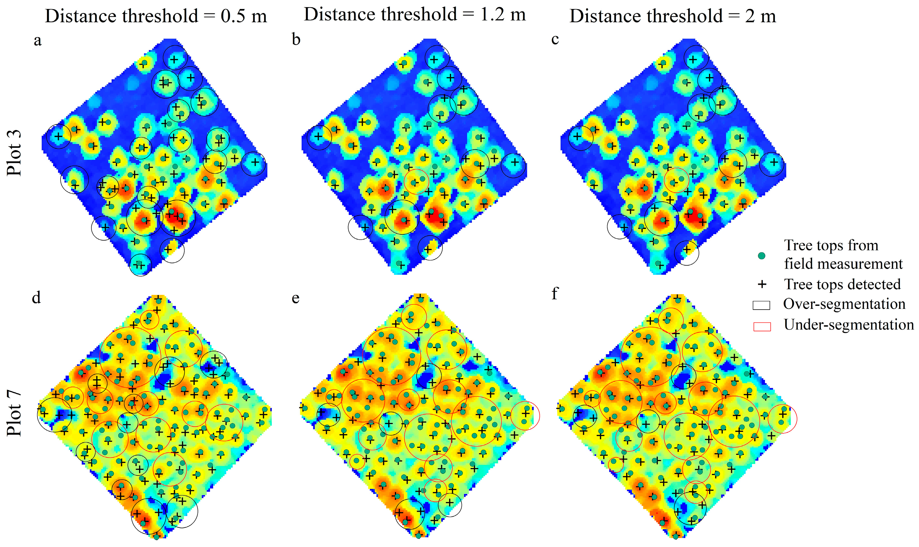
2.3.3. Euclidean Distance Clustering Algorithm

The EDCA is an algorithm that segments individual tree point clouds by a certain Euclidean distance between two trees, especially at the tops of trees. The principle of the algorithm is to find the highest point of the normalized point cloud as the crown vertex and determine the tree location and then compare and iteratively categorize the nearby points in turn. If the point is within the interval threshold, then the point will be grouped with the existing split tree. The points with a distance greater than a specified threshold distance from the target tree were excluded. First, the highest point (point A) within a tree point cloud was regarded as the tree vertex. Then, the distance was judged iteratively from tree vertex to bottom. If the horizontal distance between the target point (point B) and the point A was greater than the distance threshold, point B was categorized as another tree point cloud. Then, the next target point (point C) was determined by comparing the distance threshold. If the distance at a given point exceeded the threshold interval, the point was considered to be the vertex of another tree. Conversely, if the point was within the distance threshold, it was classified as part of the existing split tree. Finally, the steps were repeated until the bottom points were segmented. The distance is the most important parameter of this algorithm, so nine distance thresholds (0.5 m, 0.6 m, 0.8 m, 1.0 m, 1.2 m, 1.4 m, 1.6 m, 1.8 m, 2.0 m) were set according to the space of trees to investigate the optimal value for Eucalyptus plantation segmentation.

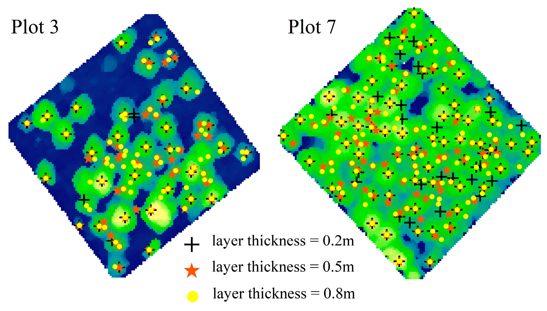
2.3.4. Layer Stacking Algorithm

The LSA method is based on the normalized point cloud data. To generate an accurate depiction of the tree boundary, the point cloud encompassing the entire stand is segmented at regular intervals. Each layer within the point cloud is analyzed to ascertain the locations of individual trees, and the results from all layers are merged to produce a representative tree boundary. First, the point cloud is layered with different layering intervals until the highest point (tree top) is reached. And the sliced point cloud is clustered to the nearest seed point and the process is repeated iteratively until the position of the seed point remained unchanged. Then, the Thiessen polygons are built in each layer according to seed points, and buffers are created to reduce clustering errors, and the polygons are stacked to produce overlapping polygons. Finally, the highest overlapping area is identified as the canopy area. It is important to note that the layer thickness used in this algorithm greatly affects the method’s ability to detect individual trees. As a result, five different layer thickness (0.2 m, 0.4 m, 0.5 m, 0.6 m, 0.8 m) were set to analyze the sensitivity of this parameter and decide the optimal value for Eucalyptus plantation segmentation.

2.4. Accuracy Assessment

The performance and sensitivity of the four segmentation algorithms were evaluated at the individual tree level by comparing with the field-observed tree heights and positions using three indices. If a segmented tree was within the boundary, it was considered correct. There are three types of segmentation results that can be produced by the evaluation. First, in the case that a tree exists and is successfully identified, it will be marked as true positive (TP), which means it has been segmented correctly. Second, in cases where a tree does exist but is not detected, it will be categorized as false negative (FN) or omission error, which is an indication of under-segmentation. Third, trees that have been detected by the algorithm but do not exist on the ground are considered false positive (FP) or commission error and represent over-segmentation. The equations are as follows [53]:
r = TP/(TP + FN)
p = TP/(TP + FP)
F = 2 × (r × p)/(r + p)
where r is the recall rate and represents detection rate; p is the precision and represents detection accuracy; and F is the score, which indicates overall correctness including commission error and omission error, with higher r and p leading to a higher F-score, indicating higher overall correctness.

3. Results

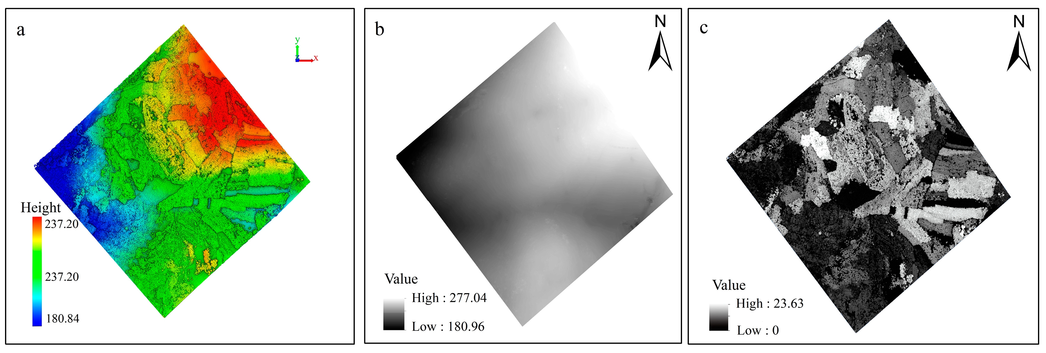
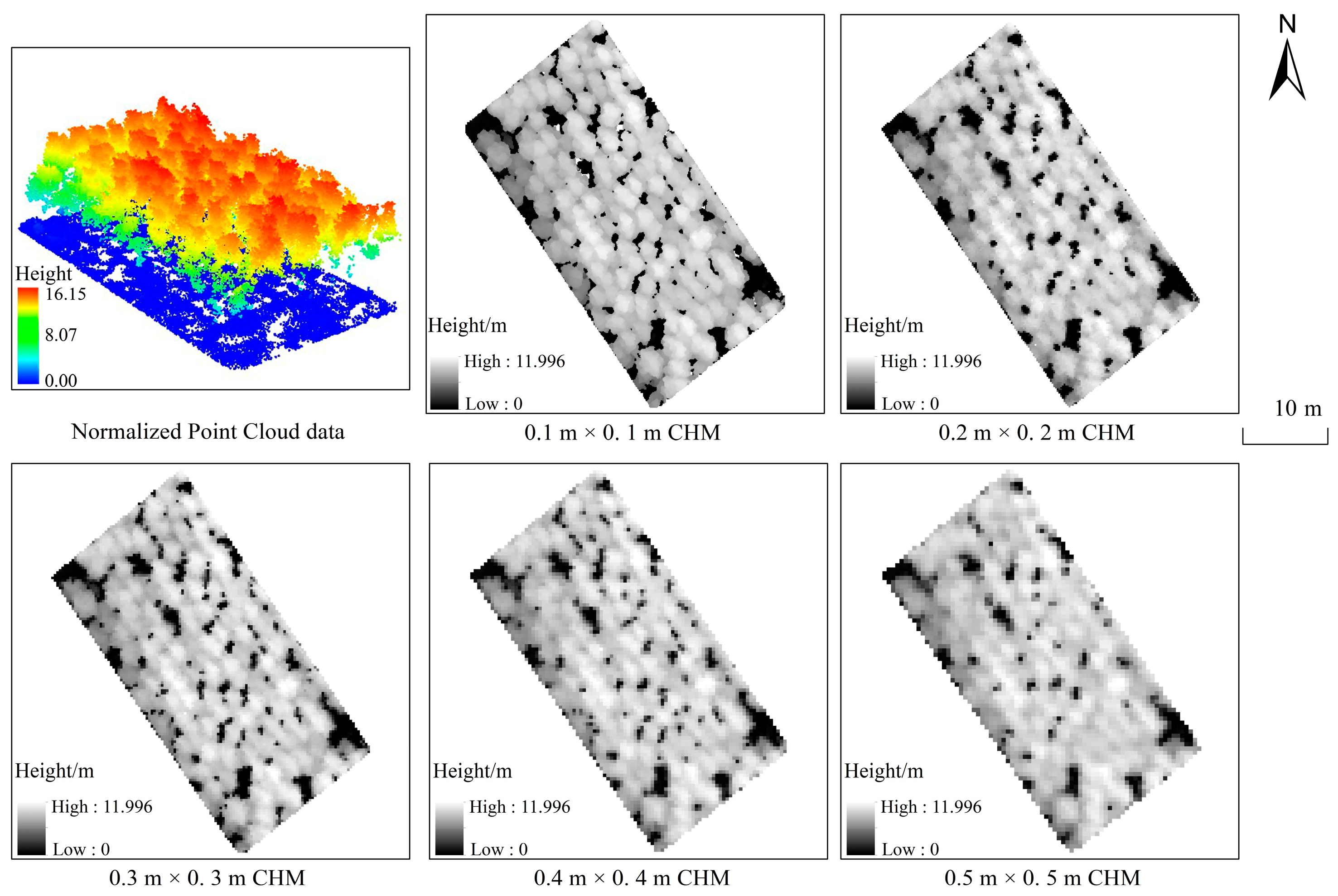
3.1. The Generation of Two Data Models

The normalized point cloud data and the CHMs with five spatial resolutions (0.1 m, 0.2 m, 0.3 m, 0.4 m and 0.5 m) were generated from the segmentation algorithms performed based on these two datasets (Figure 4). As the spatial resolution of CHM decreases, the surface details of CHM are gradually ignored. When the spatial resolution of CHM is 0.2 m × 0.2 m, it can not only fill the tiny holes on the surface of the canopy, but also display the contour among the canopy clearly. Furthermore, the brightness value among the canopy gap is obviously reduced, which enhances the canopy information and improves the precision of single-tree segmentation.

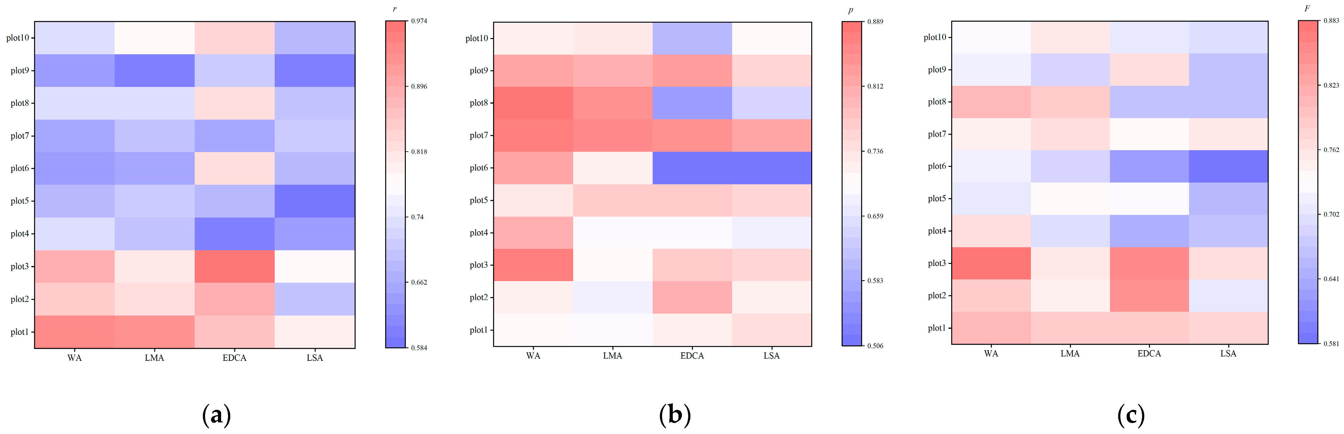
3.2. Individual Tree Segmentation

The four segmentation algorithms were applied in the ten plots separately, and the accuracy was assessed by comparing the individual tree segmentation results with the on-site position data for each tree in the sample plots (Figure 5).
The performances of four segmentation algorithms were different in the ten plots. The value of r varies from 0.585 to 0.974, and the overall value of the WA, LMA, EDCA and LSA methods was 0.729, 0.721, 0.740 and 0.672, respectively. As can be seen from Figure 5a, the r values of the first three plots were all higher than the other plots for the four segmentation algorithms. The best detection rate appeared in plot 1 for the WA, LMA and LSA methods, while for the EDCA method, the best detection rate appeared in plot 3 with the minimal density (950 n/hm2). The lowest values of the four algorithms appeared in plot 9, plot 4 and plot 5, which were high-density plots.
The value of p varies from 0.506 to 0.889. The overall value of the WA, LMA, EDCA and LSA methods was 0.797, 0.748, 0.702 and 0.704, respectively. The WA and LMA methods yielded the highest precision in plot 8. While the EDCA and LSA methods gave the highest precision in plot 7, which has the maximum density (2675 n/hm2) (Figure 5b). The lowest values of the four algorithms were obtained in plot 1, plot 2 and plot 6, which were low-density plots.
The F-score, which considers both the detection rate (r) and precision (p), varies from 0.581 to 0.883 (Figure 5c). The overall value was 0.761, 0.743, 0.720 and 0.688 for the WA, LMA, EDCA and LSA methods. The best result was obtained in plot 3 for WA, EDCA and LSA methods, while for the EDCA method, the best result appeared in plot 1.
In general, the WA method performed better than other methods as the highest p value and F were generated from this method, followed by the LMA and EDCA method with a medium detection rate and precision. The performance of the LSA method is inferior to the other methods in terms of the optimal r, p and F values. However, this method presented better results in some plots. Therefore, we further investigated how the key parameters of each algorithm affect the accuracy of individual tree segmentation.

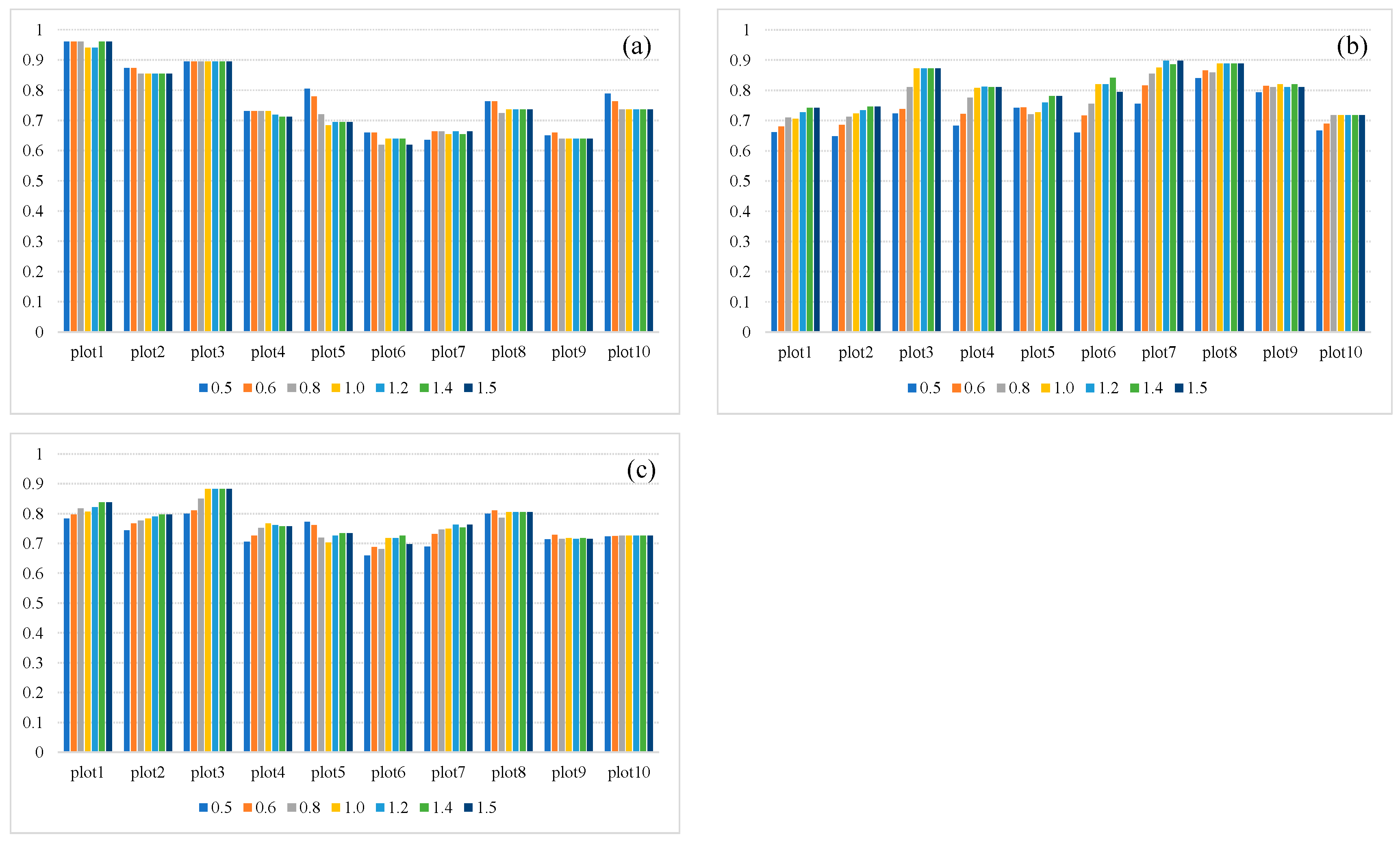
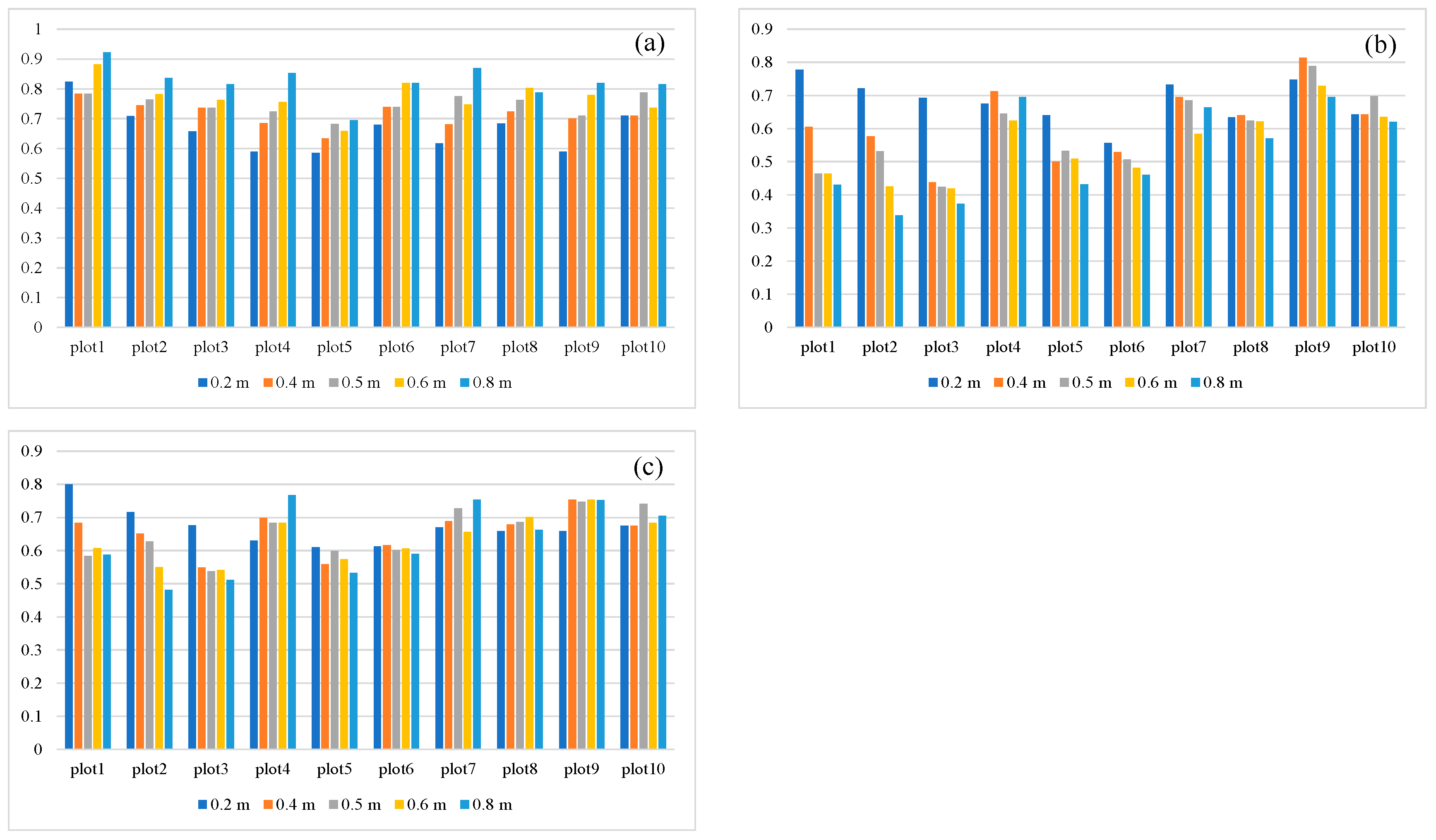
3.3. Sensitivity Analysis

3.3.1. Watershed Algorithm

To explore the influence of the key parameters on the segmentation accuracy, the Gaussian smoothing factor of the WA method was set as 0.5, 0.6, 0.8, 1.0, 1.2, 1.4 and 1.5, respectively, and the sensitivity was analyzed. The individual tree segmentation result and recall, precision and F-score were calculated for the results (Figure 6).
The detection rate of most plots presented a descending trend first and then remained stable as the Gaussian smoothing factor increased. When the Gaussian smoothing factor is set to 0.5, the r value of most plots reaches the maximum value. It is worth noting that the r value did not change in plot 3, regardless of the Gaussian smoothing factor that was applied. The variation of p and F presented a similar tendency, starting with an ascending trend, followed by stabilizing. In general, the segmentation of the canopy boundary would be finer when the value of the Gaussian smoothing factor is smaller, while larger factor values indicate coarser boundaries. The overall segmentation accuracy converges to a stable level when the Gaussian smoothing factor reaches a certain threshold.
The canopy boundary was delineated more precisely when the smoothing factor is 1 in both low-density plot and high-density plot (Figure 7a,d). Either a smaller or larger factor value would have the effect of a shrinkage or expansion of the canopy boundary.
The segmentation was more accurate in the low-density plot when the Gaussian smoothing factor is 1.5 as a smaller factor would result in over-segmentation (Figure 7c). However, when the Gaussian smoothing factor is 0.5 and 1.0, it would help to identify and segment the dwarf trees (Figure 7b).
In the high-density plot, the segmentation performance is superior when the Gaussian smoothing factor is 1.0 as can be seen from Figure 7f, the two tree canopies were identified correctly. The canopy was divided into three when the factor is 0.5, and this resulted in over-segmentation. And when the factor is 1.5, the two tree canopies were identified as one and resulted in under-segmentation. It is worth mentioning that the smaller factor value is helpful in the detection of dwarf trees.

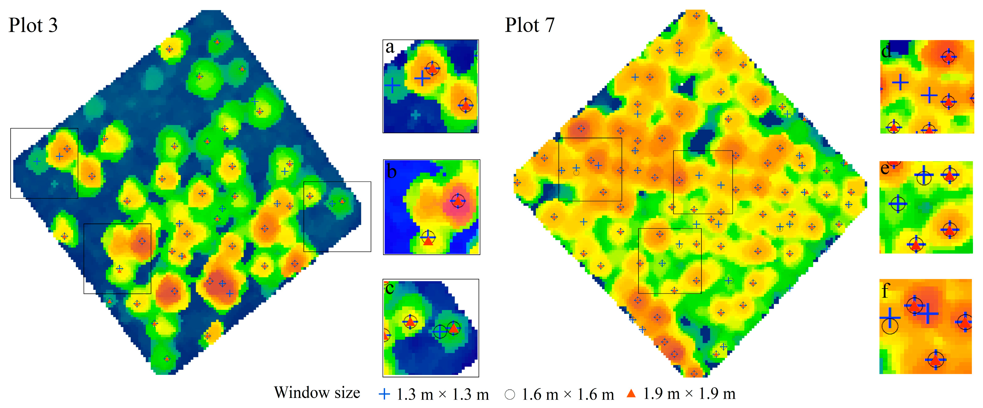
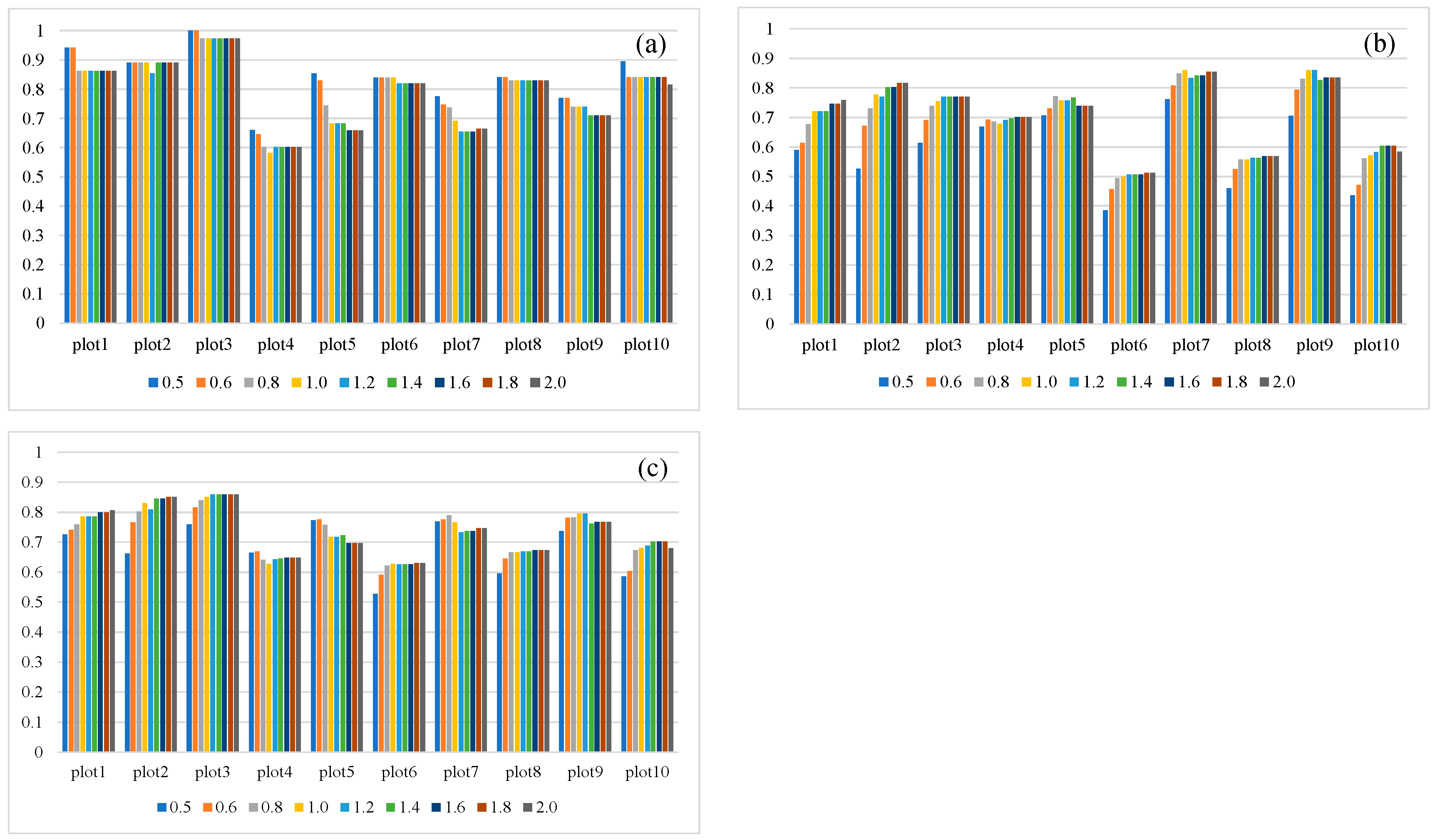
3.3.2. Local Maximum Algorithm

The window size of the LMA method was set as 1.3 m × 1.3 m, 1.6 m × 1.6 m and 1.9 m × 1.9 m, respectively, and the sensitivity was analyzed (Figure 8).
The detection rate (r) is greater for a window size of 1.3 m × 1.3 m than that for window sizes of 1.6 m × 1.6 m and 1.9 m × 1.9 m in all sample plots. The precision (p) achieved better results when the window size is 1.9 m × 1.9 m. The overall correctness of the 1.6 m × 1.6 m window size is higher compared to the other two window sizes in most of the plots.
There appears to be a relationship between the model’s ability to detect individual trees and the window size. When the window size is smaller, the individual tree detection results are better, and over-segmentation is more likely. On the contrary, the model is less capable of detecting individual trees when the window size is larger, and this increases the likelihood of under-segmentation.
When the window size is 1.3 m × 1.3 m, it is capable of identifying more tree canopies and segmenting the canopy of dwarf trees in both low-density and high-density plots (Figure 9a,d). However, it is prone to result in over-segmentation (Figure 9c,f). On the contrary, it is not able to recognize as many tree canopies when the window size is 1.9 m × 1.9 m. And it is more likely to generate under-segmentation (Figure 9e). On the other side, if the tree canopies were overlapped, it can only recognize the extreme values of the canopy, which is also under-segmentation (Figure 9b).
In general, the overall correctness is best when the window size is 1.6 m × 1.6 m in the low-density plot. While in the high-density plot, the overall correctness is best when the window size is 1.3 m × 1.3 m.

3.3.3. Euclidean Distance Clustering Algorithm

The distance between two canopy vertices is the most important factor for this method, so nine distance thresholds (0.5 m, 0.6 m, 0.8 m, 1.0 m, 1.2 m, 1.4 m, 1.6 m, 1.8 m, 2.0 m) were set to investigate the sensitivity of this factor for segmentation (Figure 10).
The detection rate r of all plots reaches the maximum value 1 when the spacing of the canopy vertex is set to 0.5 m and 0.6 m. As the distance thresholds increase, the detection rates (r) of individual trees decrease (Figure 10a), while when the spacing of canopy vertex increases to 1.2, the overall correctness (F) reaches the maximum value. And then, the overall correctness (F) stabilizes, although the spacing of canopy vertex increases (Figure 10c). The precision (p) increases as the distance thresholds increase in relatively lower density plots like plot 1, plot 2 and plot 3. But in higher density plots, like plot 5, plot 7 and plot 9, the p value increased first and then decreased as the distance thresholds increased.
As the distance between the canopy vertices was getting smaller, more trees were detected, and it was easier to be over-segmented in both low-density and high-density plots (Figure 11). As the distance threshold increased, the number of trees detected decreased, and under-segmentation became evident (Figure 11c,f).
The detection rates (r) performed best in plot 3 and reached 1 when the distance threshold was 0.5 m and 0.6 m. However, the precision (p) was most inferior correspondingly.
Compared to the low-density plot, the distance between the canopy vertices was shorter in the high-density plot. As a result, when the distance threshold was 0.5 m, the overall correctness (F) of plot 7 was better than plot 3. In general, the smaller distance threshold was more suitable for the high-density plot, and the larger distance threshold was more suitable for the low-density plot.

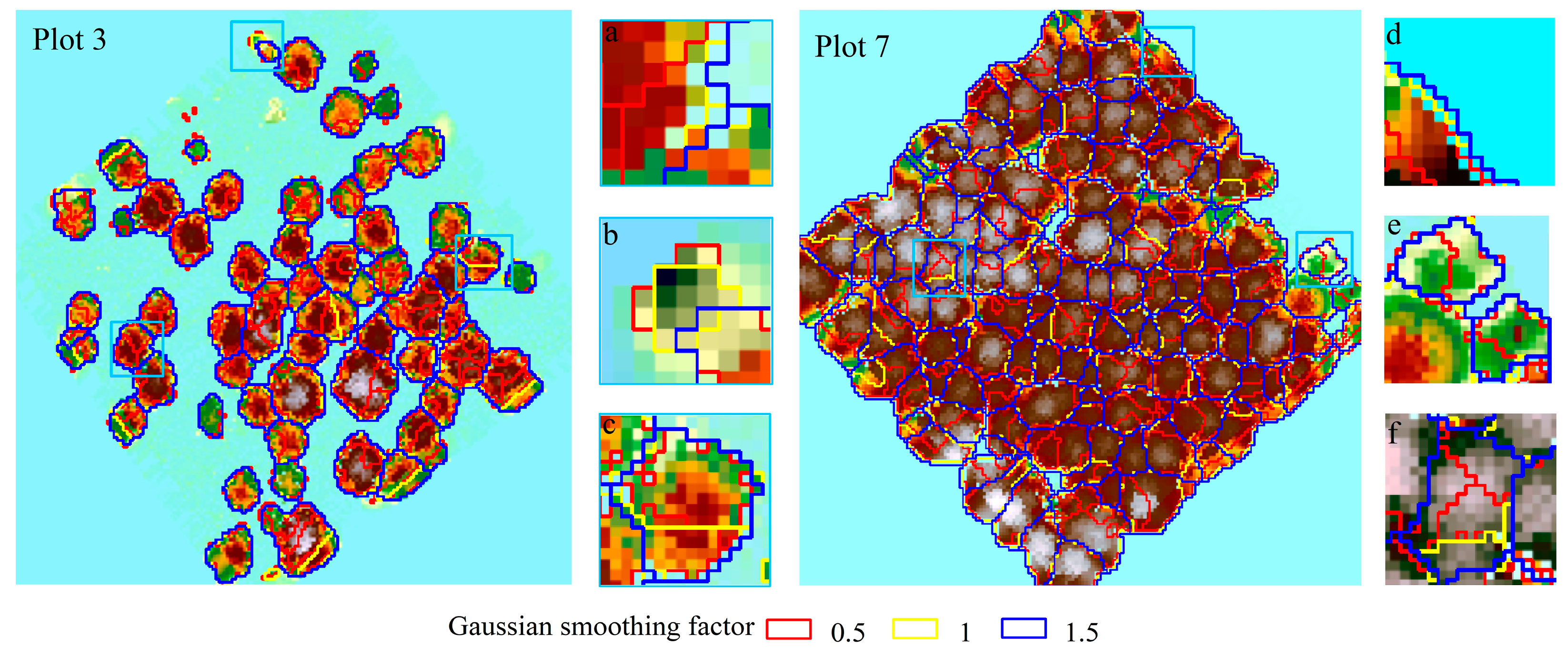
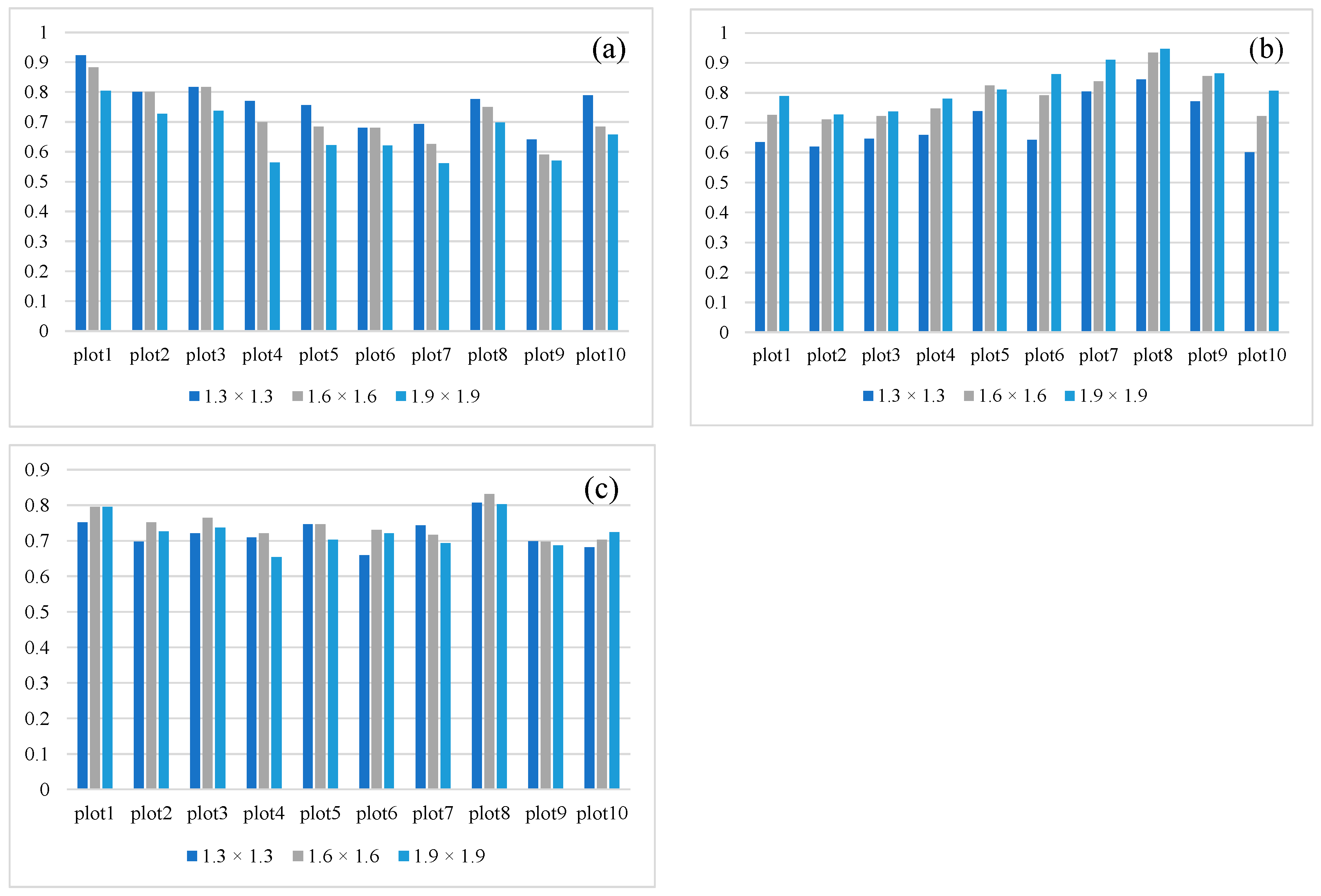
3.3.4. Layer Stacking Algorithm

Five layer thicknesses (0.2 m, 0.4 m, 0.5 m, 0.6 m, 0.8 m) were set to inquire into the sensitivity of this factor for segmentation of this method (Figure 12).
Compared to the above three segmentation algorithms, the accuracy of the LSA method is relatively low. The detection rate (r) increased as the layer thickness increased in most plots (Figure 12a), while the precision (p) presented a decreasing trend as the layer thickness increased (Figure 12b). The overall correctness (F) showed a descending trend in lower density plots and an ascending trend in most higher density plots (Figure 12c). The optimal F value is 0.8 which appeared in plot 1 with a layer thickness of 0.2 m.
Most trees were segmented correctly when the layer thickness is 0.2 m in both the low-density plot and high-density plot. When the layer thickness increased, more trees were identified which resulted in over-segmentation with a higher detection rate (r) (Figure 13). However, the precision (p) was lower.
In the low-density plot, when the layer thickness is 0.2 m, the precision (p) and overall correctness (F) were optimum with values all above 0.67. In the high-density plot, the F value reached the optimal value when the layer thickness is 0.8 m.

4. Discussion

4.1. Performance of the Methods

The overall value of the detection rate (r) of the WA, LMA, EDCA and LSA methods was 0.729, 0.721, 0.740 and 0.672, respectively, which indicated that there was no significant difference in the detection results of the four methods. However, the difference between the low-density plots and high-density plots was obvious. As the detection rates (r) for low-density plots of the four methods were 0.815, 0.802, 0.875 and 0.728. While for high-density plots, the detection rates were 0.691, 0.685, 0.680 and 0.647, respectively. The tree density and tree spacing were the key parameters influencing the identifying of individual trees. This is consistent with the findings of Yang et al. [54], who discovered that the uncertainty in tree spacing thresholds within dense stands makes them susceptible to over-segmentation. Koch et al., Vauhkonen et al. and Zawawi et al. also found that the stand density was correlated with identification of individual trees [42,55,56]. In dense deciduous forests, the continuous canopy affected individual tree detection rates, resulting in lower segmentation accuracy. Moreover, Li et al. also explored the effect of tree spacing on segmentation results [53]. The results indicated that compared to the dense plot, the detection rate was higher in the sparse plot, which is in accordance with our results.
Unlike the detection rates (r), the precision (p) of low-density plots was lower compared to the high-density plots. And the segmentation methods based on CHMs (p = 0.797 and 0.748) performed better than those based on normalized point cloud data (p = 0.702 and 0.704). In terms of overall correctness (F), the segmentation methods based on CHMs also performed better than those based on normalized point cloud data. Different from the previous studies, the CHMs in this study were generated from rasterized normalized point cloud data, which avoided the missing canopy information during the interpolation process. Moreover, the average density of point cloud data in this study was higher compared with other studies [27,57]. And higher density point cloud data generated CHMs with a higher resolution, which in turn improved the segmentation accuracy of the WA method.

4.2. Sensitivity of the Parameters

The performance of the four methods was different in the ten plots, as the stand age, crown shape, canopy radius, stand density, row spacing and stand structure are also important factors influencing the parameter sensitivity and accuracy of segmentation.
The WA method performed best among all of the four segmentation methods (F = 0.761). The misinterpretation was most linked to complex forest stand conditions, including the overlap of canopies in mature forests like plot 6, tall shrubs and dwarf trees, and two or more plants in one hole. In addition, the crown shape of Eucalyptus is in the form of a steeple, which has discrepancies with the WA method implemented in the ideal condition. This is also supported by Peuhkurinen et al. [58], who also proposed that individual tree identification was influenced by the canopy coverage and the size of trees.
The LMA method performed better in cases where the trees were regularly arranged in the plots, which is suitable for homogeneous forests. This is also supported by Ma et al., as the study found that this method could accurately explore the positions of treetops, and better results were presented in homogeneous forests with regular crown shapes [27].
Generally, the accuracy of individual tree segmentation algorithms based on normalized point cloud data depends on the arrangement of the trees. In high-density plots with small tree spacing, like plot 4 and plot 6, the EDCA method performed worse compared to the low-density plot with large spacing. The distance threshold was one of the most important factors that affected the accuracy of segmentation. Large or small canopy vertex distances can lead to under-segmentation or over-segmentation, respectively. The optimal distance threshold should correspond to the average crown radius. This is consistent with the findings of Li et al., where the distance threshold was the main uncertainty of the EDCA method [53]. Compared to the sparse plots, the optimal distance threshold is difficult to determine in dense stands as the tree spacing is small.
The LSA method can effectively determine the center of a tree using points from the trunk to the crown through point cloud layering, but the over-segmentation becomes evident as the segmentation layer thickness increases [19]. The reason is that the point cloud at the canopy boundary is denser than the tree center, which makes it easy to segment a tree into multiple canopies, thus reducing the segmentation accuracy, which is consistent with the findings of Ma et al., Ayrey et al. and Yang et al. [38,44,54]. In addition, the polygons formed by the clustered point clouds of the lower and upper levels have little overlap in dense and high-tree-height plots, which can lead to duplicate identification or omission of seed points and unsatisfactory segmentation results [27,44].

5. Conclusions

In this study, based on the normalized point cloud data and the CHMs generated from the original UAV-LiDAR data, four methods were applied to segment individual Eucalyptus spp. plantation. The accuracy of four segmentation algorithms was compared, and their performance in both low-density and high-density Eucalyptus plantation plots was investigated. Then, the parameter sensitivity of each segmentation method was analyzed, and the optimal segmentation algorithm and parameter settings were discussed according to the extraction accuracy.
In terms of overall correctness, the WA method performed best among all of the four segmentation methods (F = 0.761). And the segmentation methods based on CHMs (F = 0.761 and 0.734) also performed better than those based on normalized point cloud data (F = 0.720 and 0.688). Compared to the high-density plots, the detection rate (r) and overall correctness (F) was higher in low-density plots, while the precision (p) was lower in low-density plots.
The segmentation accuracy varied as the key parameter of the four methods changed. The sensitivity and performance of the methods were compared. Generally, the detection rate (r) presented a descending trend, as the gaussian smoothing factor of the WA method, the window size of LMA method and distance threshold of EDCA method increased. And only the detection rate (r) presented an ascending trend when the layer thickness of LSA method increased. Contrarily, opposite trends were observed for the precision (p). The overall correctness (F) exhibited an increasing trend in low-density plots and decreasing trend in high-density plots, as the window size and distance threshold increased. While as the layer thickness increased, the F value showed a decreasing trend in low-density plots and an increasing trend in high-density plots.
It is possible to find a satisfying performance for different types of forest plots using different individual tree segmentation methods with optimal parameters. The forest structures and individual wood characteristics are important factors influencing the parameter sensitivity. The Gaussian smoothing factor is affected by the crown shape and row spacing, and the window size is determined by the canopy size and tree height. The selection of distance thresholds depends mainly on the canopy radius and row spacing, and the layer thickness is influenced by the vertical structure of the forest stand and the tree shape. It is crucial to choose and set superior key parameters for different segmentation algorithms according to the forest stand structure to obtain robust and accurate segmentation results.
The study found satisfying performance for different types of Eucalyptus plots using different individual tree segmentation methods with optimal parameters. The segmentation methods based on CHM performed better than those based on point cloud data. And the overall segmentation results of low-density plots were better than those of high-density plots. The study was expected to provide an efficient way for Eucalyptus spp. plantation inventory. And it can be used for the construction of ecological models and three-dimensional modeling that are in need of individual tree information to better understand the forest ecosystem. In future research, with advances in recognition technology, more segmentation algorithms can be applied to explore more outcomes.

Author Contributions

Conceptualization, Y.H.; data curation, Y.H. and Y.Y.; formal analysis, J.J.; funding acquisition, Y.H. and Y.Y.; investigation, Y.Y. and J.J.; methodology, J.L.; resources, S.S.; supervision, S.S.; visualization, J.L. and J.J.; writing the original draft, Y.Y. and J.L.; writing—review and editing, S.S.; validation, J.L. All authors have read and agreed to the published version of the manuscript.

Funding

This research was funded by the National Natural Science Foundation of China (NO. 42061063); the Guangxi Key Research and Development Program (NO. 2023AB06010); and the Guangxi Science and Technology Plan Project (NO. AD20238059).

Data Availability Statement

The data presented in this study are available on request from the corresponding author.

Acknowledgments

The authors wish to thank the editors and anonymous referees for their very professional reviews and useful suggestions. The authors also thank the home-for-researchers website for improving their writing skills.

Conflicts of Interest

The authors declare no conflicts of interest.

References

  1. Hutapea, F.J.; Weston, C.J.; Mendham, D.; Volkova, L. Sustainable management of Eucalyptus pellita plantations: A review. For. Ecol. Manag. 2023, 537, 120941. [Google Scholar] [CrossRef]
  2. Turnbull, J.W. Eucalypt plantations. New For. 1999, 17, 37–52. [Google Scholar] [CrossRef]
  3. Rockwood, D.L.; Rudie, A.W.; Ralph, S.A.; Zhu, J.Y.; Winandy, J.E. Energy product options for eucalyptus species grown as short rotation woody crops. Int. J. Mol. Sci. 2008, 9, 1361–1378. [Google Scholar] [CrossRef] [PubMed]
  4. Zhang, C.; Xiao, X.; Zhao, L.; Qin, Y.; Doughty, R.; Wang, X.; Dong, J.; Yang, X. Mapping Eucalyptus plantation in Guangxi, China by using knowledge-based algorithms and PALSAR-2, Sentinel-2, and Landsat images in 2020. Int. J. Appl. Earth Obs. Geoinf. 2023, 120, 103348. [Google Scholar] [CrossRef]
  5. Zhang, H.; Guan, D.; Song, M. Biomass and carbon storage of eucalyptus and Acacia plantations in the Pearl River Delta, South China. For. Ecol. Manag. 2012, 277, 90–97. [Google Scholar] [CrossRef]
  6. McRoberts, R.E.; Tomppo, E.O.; Næsset, E. Advances and emerging issues in national forest. Scand. J. For. Res. 2010, 25, 368–381. [Google Scholar] [CrossRef]
  7. Hamraz, H.; Contreras, M.A.; Zhang, J. A robust approach for tree segmentation in deciduous forests using small-footprint airborne LiDAR data. Int. J. Appl. Earth Obs. Geoinf. 2016, 52, 532–541. [Google Scholar] [CrossRef]
  8. Corona, P.; Chirici, G.; McRoberts, R.E.; Winter, S.; Barbati, A. Contribution of large-scale forest inventories to biodiversity assessment and monitoring. For. Ecol. Manag. 2011, 262, 2061–2069. [Google Scholar] [CrossRef]
  9. Qin, H.; Zhou, W.; Yao, Y.; Wang, W. Individual tree segmentation and tree species classification in subtropical broadleaf forests using UAV-based LiDAR, hyperspectral, and ultrahigh-resolution RGB data. Remote Sens. Environ. 2022, 280, 113143. [Google Scholar] [CrossRef]
  10. Kellner, J.R.; Armston, J.; Birrer, M.; Cushman, K.C.; Duncanson, L.; Eck, C.; Falleger, C.; Imbach, B.; Kral, K.; Krucek, M.; et al. New opportunities for forest remote sensing through ultra-high-density drone lidar. Surv. Geophys. 2019, 40, 959–977. [Google Scholar] [CrossRef]
  11. Magnussen, S.; Nord-Larsen, T.; Riis-Nielsen, T. Lidar supported estimators of wood volume and aboveground biomass from the Danish national forest inventory (2012–2016). Remote Sens. Environ. 2018, 211, 146–153. [Google Scholar] [CrossRef]
  12. Wang, Y.; Hyyppä, J.; Liang, X.; Kaartinen, H.; Yu, X.; Lindberg, E.; Holmgren, J.; Qin, Y.; Mallet, C.; Ferraz, A.; et al. International Benchmarking of the Individual tree detection methods for modeling 3-D canopy structure for silviculture and forest ecology using airborne laser scanning. IEEE Trans. Geosci. Remote Sens. 2016, 54, 5011–5027. [Google Scholar] [CrossRef]
  13. Hu, T.; Sun, X.; Su, Y.; Guan, H.; Sun, Q.; Kelly, M.; Guo, Q. Development and performance evaluation of a very low-cost UAV-Lidar system for forestry applications. Remote Sens. 2020, 13, 77. [Google Scholar] [CrossRef]
  14. Zheng, G.; Moskal, L.M. Retrieving leaf area index (LAI) using remote sensing: Theories, methods and sensors. Sensors 2009, 9, 2719–2745. [Google Scholar] [CrossRef] [PubMed]
  15. Wagner, F.H.; Ferreira, M.P.; Sanchez, A.; Hirye, M.C.; Zortea, M.; Gloor, E.; Phillips, O.L.; Filho, C.R.S.; Shimabukuro, Y.E.; Aragão, L.E. Individual tree crown delineation in a highly diverse tropical forest using very high resolution satellite images. ISPRS J. Photogramm. Remote Sens. 2018, 145, 362–377. [Google Scholar] [CrossRef]
  16. You, H.; Liu, Y.; Lei, P.; Qin, Z.; You, Q. Segmentation of individual mangrove trees using UAV-based LiDAR data. Ecol. Inform. 2023, 77, 102200. [Google Scholar] [CrossRef]
  17. Hamraz, H.; Contreras, M.A.; Zhang, J. Vertical stratification of forest canopy for segmentation of understory trees within small-footprint airborne LiDAR point clouds. ISPRS J. Photogramm. Remote Sens. 2017, 130, 385–392. [Google Scholar] [CrossRef]
  18. Cao, L.; Coops, N.C.; Sun, Y.; Ruan, H.; Wang, G.; Dai, J.; She, G. Estimating canopy structure and biomass in bamboo forests using airborne LiDAR data. ISPRS J. Photogramm. Remote Sens. 2019, 148, 114–129. [Google Scholar] [CrossRef]
  19. Chen, Q.; Gao, T.; Zhu, J.; Wu, F.; Li, X.; Lu, D.; Yu, F. Individual tree segmentation and tree height estimation using leaf-off and leaf-on UAV-LiDAR data in dense deciduous forests. Remote Sens. 2022, 14, 2787. [Google Scholar] [CrossRef]
  20. Popescu, S.C. Estimating biomass of individual pine trees using airborne lidar. Biomass Bioenergy 2007, 31, 646–655. [Google Scholar] [CrossRef]
  21. Næsset, E. Predicting forest stand characteristics with airborne scanning laser using a practical two-stage procedure and field data. Remote Sens. Environ. 2002, 80, 88–99. [Google Scholar] [CrossRef]
  22. Bouvier, M.; Durrieu, S.; Fournier, R.A.; Renaud, J.P. Generalizing predictive models of forest inventory attributes using an area-based approach with airborne LiDAR data. Remote Sens. Environ. 2015, 156, 322–334. [Google Scholar] [CrossRef]
  23. Vastaranta, M.; Kankare, V.; Holopainen, M.; Yu, X.; Hyyppä, J.; Hyyppä, H. Combination of individual tree detection and area-based approach in imputation of forest variables using airborne laser data. ISPRS J. Photogramm. Remote Sens. 2012, 67, 73–79. [Google Scholar] [CrossRef]
  24. Næsset, E. Practical large-scale forest stand inventory using a small-footprint airborne scanning laser. Scand. J. For. Res. 2004, 19, 164–179. [Google Scholar] [CrossRef]
  25. Means, J.E.; Acker, S.A.; Fitt, B.J.; Renslow, M.; Emerson, L.; Hendrix, C.J. Predicting Forest Stand Characteristics with Airborne Scanning Lidar. Photogramm. Eng. Remote Sens. 2000, 66, 1367–1371. [Google Scholar]
  26. Yu, X.; Hyyppä, J.; Holopainen, M.; Vastaranta, M. Comparison of Area-Based and Individual Tree-Based Methods for Predicting Plot-Level Forest Attributes. Remote Sens. 2010, 2, 1481–1495. [Google Scholar] [CrossRef]
  27. Ma, K.; Chen, Z.; Fu, L.; Tian, W.; Jiang, F.; Yi, J.; Du, Z.; Sun, H. Performance and sensitivity of individual tree segmentation methods for UAV-LiDAR in multiple forest types. Remote Sens. 2022, 14, 298. [Google Scholar] [CrossRef]
  28. Wu, X.; Shen, X.; Cao, L.; Wang, G.; Cao, F. Assessment of individual tree detection and canopy cover estimation using unmanned aerial vehicle based light detection and ranging (UAV-LiDAR) data in planted forests. Remote Sens. 2019, 11, 908. [Google Scholar] [CrossRef]
  29. Yao, W.; Krzystek, P.; Heurich, M. Tree species classification and estimation of stem volume and DBH based on single tree extraction by exploiting airborne full-waveform LiDAR data. Remote Sens. Environ. 2012, 123, 368–380. [Google Scholar] [CrossRef]
  30. Shinzato, E.T.; Shimabukuro, Y.E.; Coops, N.C.; Tompalski, P.; Gasparoto, E.A. Integrating area-based and individual tree detection approaches for estimating tree volume in plantation inventory using aerial image and airborne laser scanning data. iForest 2016, 10, 296. [Google Scholar] [CrossRef]
  31. Hyyppä, J.; Hyyppä, H.; Leckie, D.; Gougeon, F.; Yu, X.; Maltamo, M. Review of methods of small-footprint airborne laser scanning for extracting forest inventory data in boreal forests. Int. J. Remote Sens. 2008, 29, 1339–1366. [Google Scholar] [CrossRef]
  32. Hall, S.A.; Burke, I.C.; Box, D.O.; Kaufmann, M.R.; Stoker, J.M. Estimating stand structure using discrete-return lidar: An example from low density, fire prone ponderosa pine forests. For. Ecol. Manag. 2005, 208, 189–209. [Google Scholar] [CrossRef]
  33. Qin, Y.; Ferraz, A.; Mallet, C.; Iovan, C. Individual tree segmentation over large areas using airborne LiDAR point cloud and very high resolution optical imagery. In Proceedings of the 2014 IEEE Geoscience and Remote Sensing Symposium, Quebec City, QC, Canada, 13–18 July 2014; pp. 800–803. [Google Scholar]
  34. Popescu, S.C.; Wynne, R.H. Seeing the trees in the forest. Photogramm. Eng. Remote Sens. 2004, 70, 589–604. [Google Scholar] [CrossRef]
  35. Chen, Q.; Baldocchi, D.; Gong, P.; Kelly, M. Isolating individual trees in a savanna woodland using small footprint lidar data. Photogramm. Eng. Remote Sens. 2006, 72, 923–932. [Google Scholar] [CrossRef]
  36. Wang, L.; Gong, P.; Biging, G.S. Individual tree-crown delineation and treetop detection in high-spatial-resolution aerial imagery. Photogramm. Eng. Remote Sens. 2004, 70, 351–357. [Google Scholar] [CrossRef]
  37. Heurich, M. Automatic recognition and measurement of single trees based on data from airborne laser scanning over the richly structured natural forests of the Bavarian Forest National Park. For. Ecol. Manag. 2008, 255, 2416–2433. [Google Scholar] [CrossRef]
  38. Ma, K.; Xiong, Y.; Jiang, F.; Chen, S.; Sun, H. A novel vegetation point cloud density tree-segmentation model for overlapping crowns using UAV LiDAR. Remote Sens. 2021, 13, 1422. [Google Scholar] [CrossRef]
  39. Jing, L.; Hu, B.; Noland, T.; Li, J. An individual tree crown delineation method based on multi-scale segmentation of imagery. ISPRS J. Photogramm. Remote Sens. 2012, 70, 88–98. [Google Scholar] [CrossRef]
  40. Balsi, M.; Esposito, S.; Fallavollita, P.; Nardinocchi, C. Single-tree detection in high-density LiDAR data from UAV-based survey. Eur. J. Remote Sens. 2018, 51, 679–692. [Google Scholar] [CrossRef]
  41. Zaforemska, A.; Xiao, W.; Gaulton, R. Individual tree detection from UAV LiDAR data in a mixed species woodland. Int. Arch. Photogramm. Remote Sens. Spat. Inf. Sci. 2019, XLII-2/W13, 657–663. [Google Scholar] [CrossRef]
  42. Koch, B.; Heyder, U.; Weinacker, H. Detection of individual tree crowns in airborne lidar data. Photogramm. Eng. Remote Sens. 2006, 72, 357–363. [Google Scholar] [CrossRef]
  43. Hu, X.; Chen, W.; Xu, W. Adaptive Mean Shift-Based Identification of Individual Trees Using Airborne LiDAR Data. Remote Sens. 2017, 9, 148. [Google Scholar] [CrossRef]
  44. Ayrey, E.; Fraver, S.; Kershaw, J.A.; Kenefic, L.S.; Hayes, D.; Weiskittel, A.R.; Roth, B.E. Layer Stacking: A novel algorithm for individual forest tree segmentation from LiDAR point clouds. Can. J. Remote Sens. 2016, 43, 16–27. [Google Scholar] [CrossRef]
  45. Morsdorf, F.; Meier, E.; Kötz, B.; Itten, K.I.; Dobbertin, M.; Allgöwer, B. LiDAR-based geometric reconstruction of boreal type forest stands at single tree level for forest and wildland fire management. Remote Sens. Environ. 2004, 92, 353–362. [Google Scholar] [CrossRef]
  46. Lu, X.; Guo, Q.; Li, W.; Flanagan, J. A bottom-up approach to segment individual deciduous trees using leaf-off lidar point cloud data. ISPRS J. Photogramm. Remote Sens. 2014, 94, 1–12. [Google Scholar] [CrossRef]
  47. Shendryk, I.; Broich, M.; Tulbure, M.G.; Alexandrov, S.V. Bottom-up delineation of individual trees from full-waveform airborne laser scans in a structurally complex eucalypt forest. Remote Sens. Environ. 2016, 173, 69–83. [Google Scholar] [CrossRef]
  48. Alexander, C. Delineating tree crowns from airborne laser scanning point cloud data using Delaunay triangulation. Int. J. Remote Sens. 2009, 30, 3843–3848. [Google Scholar] [CrossRef]
  49. Duan, Z.; Zhao, D.; Zeng, Y.; Zhao, Y.; Wu, B.; Zhu, J. Assessing and Correcting Topographic Effects on Forest Canopy Height Retrieval Using Airborne LiDAR Data. Sensors 2015, 15, 12133–12155. [Google Scholar] [CrossRef]
  50. Yin, D.; Wang, L. Individual mangrove tree measurement using UAV-based LiDAR data Possibilities and challenges. Remote Sens. Environ. 2019, 223, 34–49. [Google Scholar] [CrossRef]
  51. Xie, Y.; Chen, Y.; Zhang, Y.; Li, M.; Xie, M.; Mo, W. Response of vegetation normalized different vegetation index to different meteorological disaster indexes in karst region of Guangxi, China. Heliyon 2023, 9, e20518. [Google Scholar] [CrossRef]
  52. Vincent, L.; Soille, P. Watersheds in digital spaces: An efficient algorithm based on immersion simulations. IEEE Trans. Pattern Anal. Mach. Intell. 1991, 13, 583–598. [Google Scholar] [CrossRef]
  53. Li, W.; Guo, Q.; Jakubowski, M.K.; Kelly, M. A new method for segmenting individual trees from the lidar point cloud. Photogramm. Eng. Remote Sens. 2012, 78, 75–84. [Google Scholar] [CrossRef]
  54. Yang, Q.; Su, Y.; Jin, S.; Kelly, M.; Hu, T.; Ma, Q.; Li, Y.; Song, S.; Zhang, J.; Xu, G.; et al. The influence of vegetation characteristics on individual tree segmentation methods with airborne LiDAR data. Remote Sens. 2019, 11, 2880. [Google Scholar] [CrossRef]
  55. Vauhkonen, J.; Ene, L.; Gupta, S.; Heinzel, J.; Holmgren, J.; Pitkänen, J.; Solberg, S.; Wang, Y.; Weinacker, H.; Hauglin, K.M.; et al. Comparative testing of single-tree detection algorithms under different types of forest. Forestry 2012, 85, 27–40. [Google Scholar] [CrossRef]
  56. Zawawi, A.A.; Shiba, M.; Jemali, N.J.N. Accuracy of LiDAR-based tree height estimation and crown recognition in a subtropical evergreen broad-leaved forest in Okinawa, Japan. For. Syst. 2015, 24, e002. [Google Scholar]
  57. Guerra-Hernández, J.; Cosenza, D.N.; Rodriguez, L.C.E.; Silva, M.; Tomé, M.; Díaz-Varela, R.A.; González-Ferreiro, E. Comparison of ALS-and UAV (SfM)-derived high-density point clouds for individual tree detection in Eucalyptus plantations. Int. J. Remote Sens. 2018, 39, 5211–5235. [Google Scholar] [CrossRef]
  58. Peuhkurinen, J.; Mehtätalo, L.; Maltamo, M. Comparing individual tree detection and the area-based statistical approach for the retrieval of forest stand characteristics using airborne laser scanning in Scots pine stands. Can. J. For. Res. 2011, 41, 583–598. [Google Scholar] [CrossRef]
Figure 1. The study site location.
Forests 15 00209 g001
Figure 2. The original 3D point cloud (a), DTM (b) and CHM (c) of the study area.
Forests 15 00209 g002
Figure 3. The general workflow of the study.
Forests 15 00209 g003
Figure 4. The normalized point cloud data and CHM of plot 4.
Forests 15 00209 g004
Figure 5. The results of individual tree detection in ten plots; (a) r is the detection rate, (b) p is the precision and (c) F is the overall correctness.
Forests 15 00209 g005
Figure 6. The accuracy of individual tree detection with seven smoothing factors of the WA method; (a) is the detection rate (r), (b) is the precision (p), (c) is the overall correctness (F).
Forests 15 00209 g006
Figure 7. The individual tree segmentation results in low-density (plot 3) and high-density plot (plot 7); (a,d) are boundary details; (b,e) are the under-segmentation ; (c,f) are the over-segmentation.
Forests 15 00209 g007
Figure 8. The accuracy of individual tree detection with three window sizes of the LMA method; (a) is the detection rate (r), (b) is the precision (p), (c) is the overall correctness (F).
Forests 15 00209 g008
Figure 9. The individual tree segmentation results by LMA in low-density (plot 3) and high-density plot (plot 7); (a,d) identify more tree canopies and segment the canopy of dwarf trees when size is 1.3 m × 1.3 m ; (b,e) are the under-segmentation ; (c,f) are the over-segmentation.
Forests 15 00209 g009
Figure 10. The accuracy of individual tree detection with nine distance thresholds of the EDCA method; (a) is the detection rate (r), (b) is the precision (p), (c) is the overall correctness (F).
Forests 15 00209 g010
Figure 11. The individual tree segmentation results by EDCA in low-density (plot 3) and high-density plot (plot 7); (a,d) are the segmentation result when the distance threshold is 0.5 m; (b,e) are the segmentation result when the distance threshold is 1.2 m; (c,f) are the segmentation result when the distance threshold is 2 m.
Forests 15 00209 g011
Figure 12. The accuracy of individual tree detection with five layer thicknesses of the LSA method; (a) is the detection rate (r), (b) is the precision (p), (c) is the overall correctness (F).
Forests 15 00209 g012
Figure 13. The individual tree segmentation results by LSA in low-density (plot 3) and high-density plot (plot 7).
Forests 15 00209 g013
Table 1. Summary of sample plots in the study site.
VariablesMinimumMaximumMean ValueStandard Deviation
Number of treesn = 753
DBH/cm2.5015.807.762.81
Tree Height/m3.5718.0010.173.01
Crown/m1.203.802.100.46
Disclaimer/Publisher’s Note: The statements, opinions and data contained in all publications are solely those of the individual author(s) and contributor(s) and not of MDPI and/or the editor(s). MDPI and/or the editor(s) disclaim responsibility for any injury to people or property resulting from any ideas, methods, instructions or products referred to in the content.

