Three Censuses of a Mapped Plot in Coastal California Mixed-Evergreen and Redwood Forest

Abstract

Large, mapped forest research plots are important sources of data to understand spatial and temporal changes in forest communities in the context of global change. Here, we describe the data from the first three censuses of the 16-ha UC Santa Cruz Forest Ecology Research Plot, located in the Mediterranean-climate forest on the central coast of California, USA. The forest includes both mixed-evergreen forest and redwood-dominated forest and is recovering from significant logging disturbances in the early 20th century. Each woody stem with a diameter ≥ 1 cm at 1.3 m was mapped, tagged, identified, and measured, with censuses performed at ~5-year intervals. The first census included just 6 ha (previously described), and the area was then expanded to 16 ha in the second census. We describe the temporal dynamics of the forest in the original 6 ha, as well as the structure and temporal dynamics of the full 16 ha. The community includes 34 woody species, including 4 gymnosperm and 9 angiosperm tree species, 18 species of shrubs, and 3 species of lianas. The community includes eight non-native species, representing less than 0.5% of the stems. More than half the species show greater rates of mortality than recruitments, reflective of a dynamic forest community. Over a decade, the number of living woody stems has declined, but the basal area has increased, reflecting a self-thinning process.

1. Introduction

Forest ecosystems around the world are experiencing rapid changes associated with succession following harvest or other land-use changes [1,2,3], fragmentation [4,5,6], invasion by non-native plants [7,8,9], the emergence of novel pests and pathogens [10,11,12], changes in disturbance regimes [13,14,15], pollution [16,17,18], elevated levels of atmospheric CO₂ [13,19,20], and new patterns of temperature and precipitation associated with global climate change [21,22,23]. The long-term monitoring of forest plots is essential to document such changes and to understand the underlying ecological mechanisms and consequences. Forest-monitoring efforts take numerous, complementary forms, including networks of large distributed networks of plots of small size (<1 ha) (e.g., USDA Forest Inventory and Analysis plots [24], ForestPlots.net [25], EU-Forest [26]) and networks of large-scale (to 50 ha or more) mapped plots (e.g., ForestGEO network [27]). Here, we describe the forest structure and dynamics based on over a decade of censuses in a mapped 16 ha forest plot in coastal California, USA, that is part of the ForestGEO network.

The ForestGEO network includes mapped forest dynamics plots at 77 forest sites in 29 countries, incorporating more than 7.33 million trees (diameter ≥ 1 cm) and 12,000 species [27,28]. The plots cover the breadth of the forested biomes, from wet tropical forests to boreal forests [29]. Forests in the Mediterranean climate zone, which is characterized by mild, wet winters and warm, dry summers, are underrepresented in the network. Mediterranean climate regions border the Mediterranean Sea in southern Europe and northern Africa and are also found along central Chile in South America, the Cape Region of South Africa, western Australia, and the California coast in North America [30]. These regions are important biodiversity hotspots, with extensive grassland, shrubland, and forest communities. Currently, the only Mediterranean-climate plot in the ForestGEO network is the University of California Santa Cruz Forest Ecology Research Plot (FERP) [31].

The UC Santa Cruz FERP was established as a 6 ha plot in 2007 in a mixed-evergreen coastal California forest [31]. Following a second census in 2012, we expanded the FERP to 16 ha to include coastal redwood forest habitat. The complete 16 ha FERP was then censused again beginning in 2017. Located on the protected Campus Natural Reserve on the campus of UC Santa Cruz (UCSC) and only a short walk from academic classrooms and laboratories, the FERP serves two equally important roles: as a platform for research in forest ecology and as a resource for outdoor teaching and for student experiential learning.

The purpose of this paper is to provide a general overview of the UCSC FERP across the first three censuses, to make the data broadly available for comparative studies with other large plots, and to serve as the basis for site-based ecological research. We intentionally do not set out to test specific hypotheses, instead aiming to provide the necessary background for future papers that can be written using data from the plot. We describe the overall scope and characteristics of the site, as well as spatial and temporal patterns of the abundance, basal area, diversity, size distribution, mortality, recruitment, and growth for a decade of study on the University of California Forest Ecology Research Plot.

2. Materials and Methods

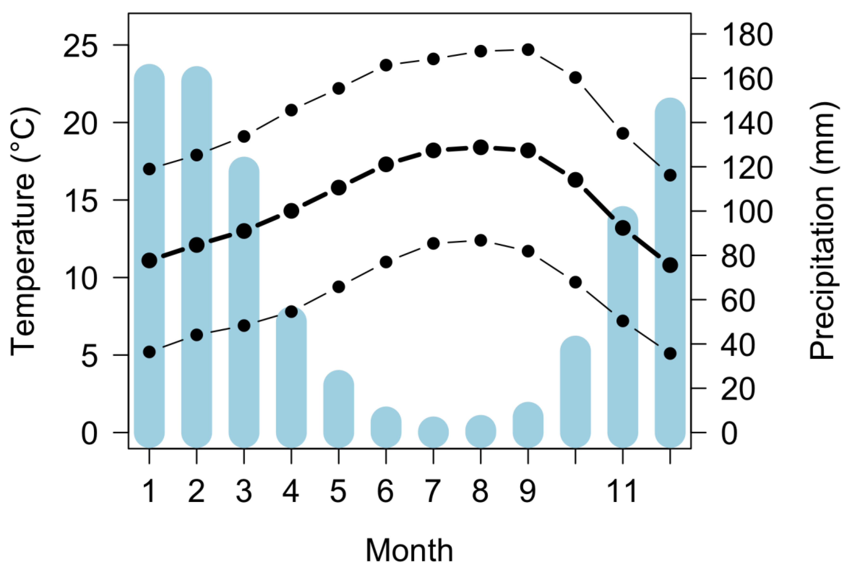
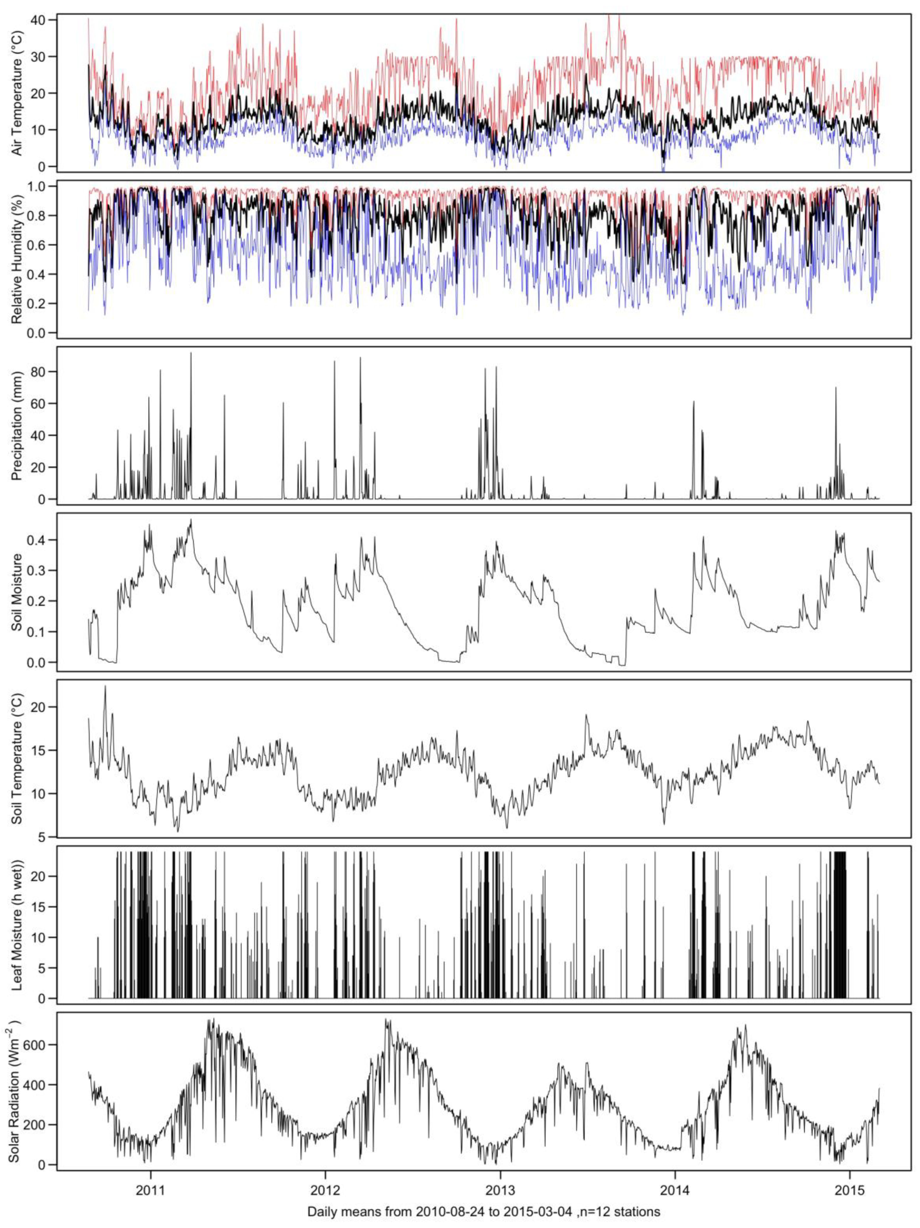
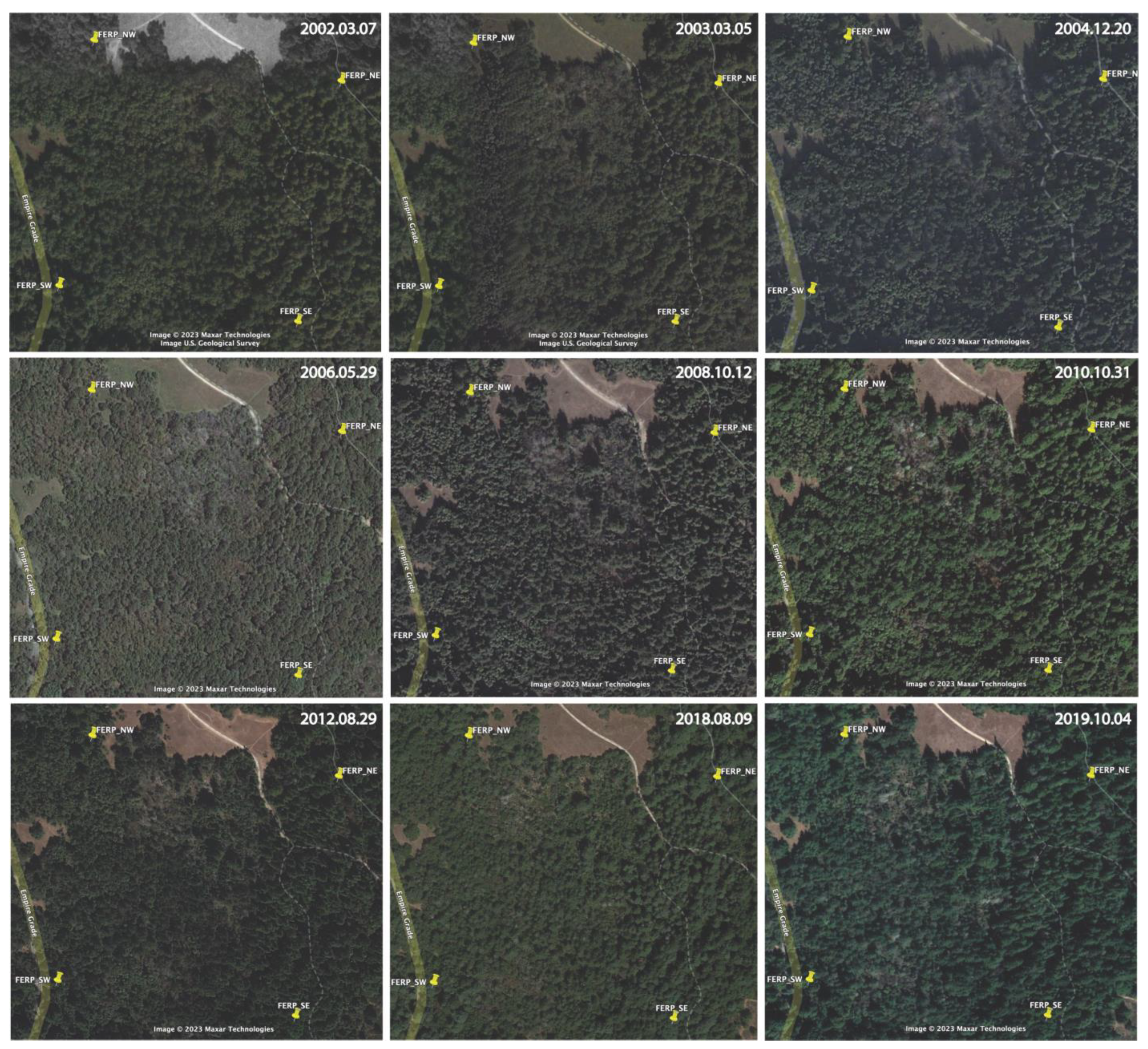
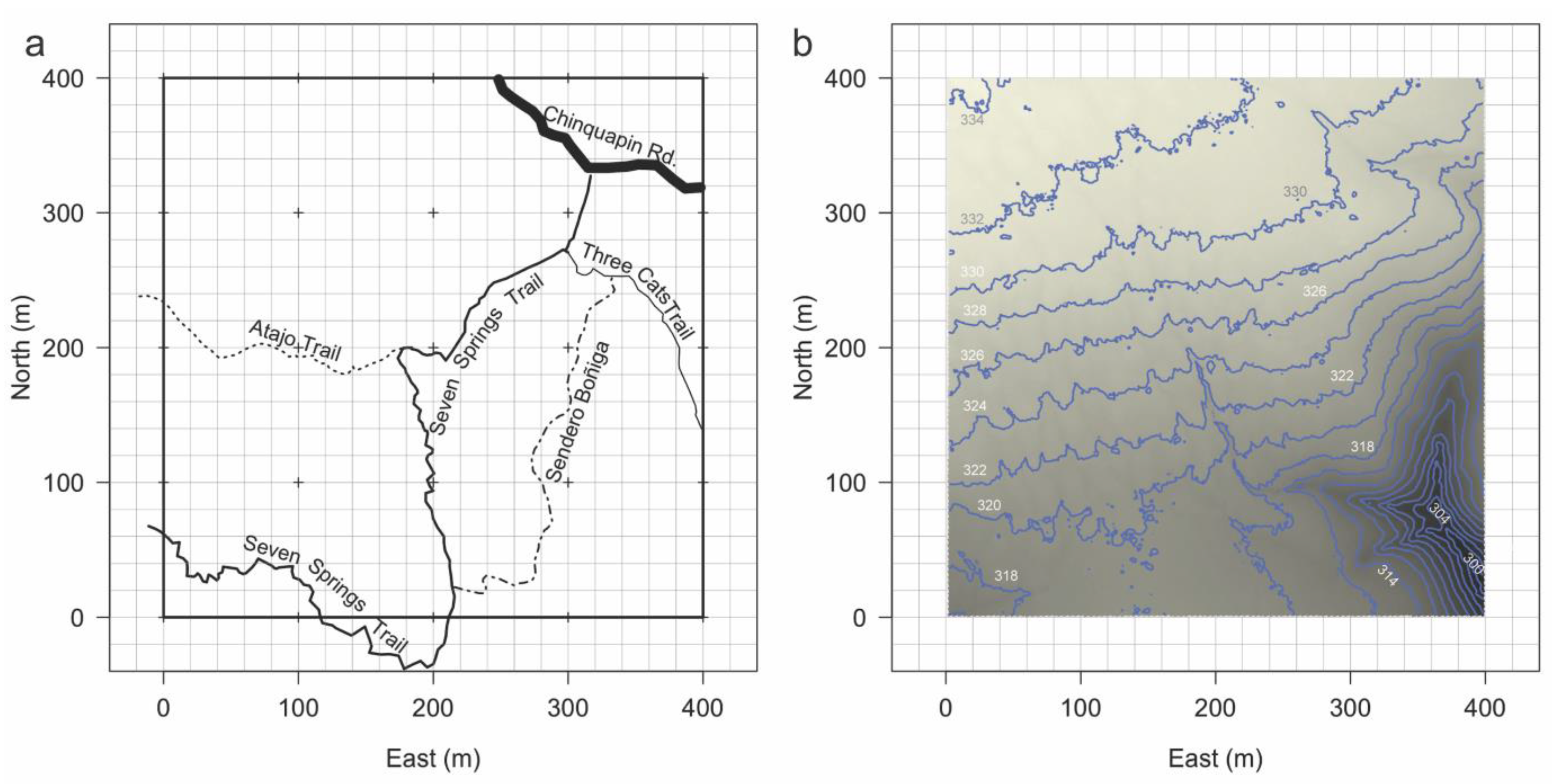
2.1. Site Description

The 16 ha UC Santa Cruz Forest Ecology Research Plot is part of the 319 ha Campus Natural Reserve on the campus of the University of California Santa Cruz. Located 7 km from the Pacific coast in the Santa Cruz Mountains, the site ranges in elevation between 296 and 335 m above sea level (masl). The topography is generally flat, with a gentle, uphill slope to the north, with a small, semi-permanent stream (significant flow only during rainy periods) draining through a deep ravine in the southeast corner (Figure 1). The southwest corner of the FERP is at 37.012416, −122.074833 (UTM 582305.3 east, 4096649.8 north, zone 10, WGS84). The plot extends 400 m east and north of that corner and is oriented to magnetic north.

The western half of the FERP is a mixed-evergreen forest dominated by conifers (mostly Pseudotsuga menziesii, Douglas-fir) and several species in the Fagaceae family. The eastern half is more conifer-dominated, with abundant Sequoia sempervirens (coast redwood) and Douglas-fir. The FERP, and the Campus Natural Reserve, is surrounded on three sides by extensive protected areas: Pogonip Open Space to the east, Henry Cowell State Park to the north, and Wilder Ranch State Park to the west. About 100 m south of the FERP is a low-density housing area (Cave Gulch), established in the mid-19th century. The academic buildings of the UCSC campus are 1.4 km to the southeast of the FERP, with protected forest and chaparral habitat between them. A two-lane road (Empire Grade) passes near the western border of the FERP, with similar forested vegetation on the other side of the road. Single-lane fire-access roads traverse the Campus Natural Reserve, including Chinquapin Road, which cuts through the northeast corner of the FERP.

The UCSC campus, including the FERP, is on the unceded territory of the Awaswas-speaking Uypi Tribe. The campus is located on the sacred homelands of the Uypi, who had a long history (10,000 years or more) of presence and active stewardship through cultural burns and other methods to support healthy ecosystems before their peoples were forcibly taken to the missions in the late 18th century [32]. The Amah Mutsun Tribal Band, comprising the descendants of indigenous people taken to Missions Santa Cruz and San Juan Bautista during the Spanish colonization of the Central Coast, is today working hard to restore traditional stewardship practices on these lands and heal from historical trauma.

The UCSC campus is on lands that had been part of the 1840s’ Mexican land grant to Pedro Sainsevain called Rancho Cañada del Rincón en el Río San Lorenzo [33]. The property was eventually purchased by Henry Cowell in 1865 and became part of the 2600 ha Cowell Ranch. Ranch activities included marble quarries and lime kilns, cattle ranching, and logging; most of the forest on the campus was clear-cut to fuel the kilns, which were in use until 1920. Active management of the ranch ceased in 1946, and in 1961, 810 ha of the ranch became the UCSC campus. As a result of clearcutting during the ranch period, cut redwood stumps with century-old resprouts are common on the eastern part of the FERP. Evidence of clearcutting is absent on the western part of the FERP, where there are few redwoods. Coring of the largest trees suggests that the forest has been largely undisturbed since the 1930s, with some trees dating back to the turn of the 20th century [31].

Wildfires and culturally set fires are normal parts of the coastal mixed-evergreen and redwood forests. A low-intensity wildfire burned through parts of the eastern extent of the FERP in 1964 [34], but there are no fire scars or clear evidence of burning in the western part of the FERP. The FERP was spared in the devastating 2020 CZU Lightning Complex fire, which burned to within about 2 km northwest of the FERP.

Santa Cruz experiences a mild, Mediterranean-type climate, with cool, moist winters and warm, dry summers. Some 98% of the annual average 796 mm of precipitation falls between October and May (Figure A1). Average daily high temperatures range from 16.6 °C in December to 24.7 °C in September; average daily low temperatures range from 5.1 °C in December to 12.4 °C in August. Most precipitation falls as rain, although marine-layer fog reaches the redwood forest regularly in the summer months. From 2010 to 2015, we maintained 12 Decagon EM50 micrometeorology stations at points across the FERP, collecting data on air temperature and relative humidity, soil temperature and moisture, precipitation, leaf moisture, and solar radiation; daily summaries of the averages of those 12 stations are presented in Figure A2.

Additional details of the site history, geology, soils, and climate are described in a volume on the natural history of the UCSC campus [35], the UCSC Long Range Development Plan [36], and in the presentation of the 2007 census of the original 6 ha section of the FERP [31].

2.2. Mapping, Measurement, and Data Protocols

Measurement protocols for the UC Santa Cruz FERP generally follow those described for the original 6 ha extent of the FERP [31], which are based on the protocols outlined for tropical plots presented by Condit [37]. We established a 20 m grid across 16 ha (400 m × 400 m), with each grid point marked with a length of pvc pipe slipped over rebar and pounded into the ground to serve as corner posts. An aluminum tag attached to each corner post indicates its location in the plot in meters from the western and southern borders (e.g., E080_N160 indicates 80 m east and 160 m north). The 20 m × 20 m quadrats are designated by coordinates of the post in the southwest corner of the quadrat. We then mapped all living stems of woody plants with a diameter of 10 mm or larger at a standard height of 1.3 m (diameter at standard height, DSH, traditionally called DBH for diameter at breast height) onto the plot with reference to those corner posts. Corner posts and woody plants were mapped using laser rangefinders and sighting compasses, and the distances (corrected to adjust for the radius of the stem) and bearings were then trigonometrically converted to meters east and north. The original mapping of the 6 ha FERP was oriented to magnetic north in 2006, at which time the declension was +14.667 east. By 2023, it had shifted to +12.84.

Each woody plant was individually tagged with an aluminum tree tag (National Band and Tag, Newport, KY, USA, Style 245, 2 ¾” x 1” Oblong, 0.025 aluminum), with sequential numbers from 00001 to 37985. For individuals with multiple stems, each stem after the largest then received a write-on aluminum tag (Forestry Suppliers, Jackson, MS, USA, double-faced aluminum tag #79500), sequentially numbered within each individual, beginning with 2. The stem with the individual tag is considered stem 1 for that individual, but it did not receive a physical stemtag. The practice of adding stemtags for multiple stems began with the FERP2 census; in FERP1, we measured the multiple stems but did not tag them. For smaller stems, we loosely attached tags to the base of the stem with an 8 mil plastic tie and grafting tape (Forestry Suppliers, ½ inch, #79313). For stems larger than 30 cm in diameter, tags were attached to the tree with aluminum nails at a height of about 2 m on the north side of the tree.

The diameter at standard height (DSH) of stems was measured at 1.3 m from the base of the stem, beginning on the side where the ground was highest. When stems were leaning or bent, the measured distance followed the growth pattern of the stem. Plastic calipers were used to measure stems smaller than 8 cm. For larger stems, the diameter was measured using diameter tapes (with scales indicating the circumference divided by pi). Measurements were recorded to the mm, rounding down. The heights of measurement points with irregularities at the standard height were adjusted following the recommendations in Condit [37].

We recorded each observed stem as living or dead but only measured the diameter of living stems. Additional observations of dead trees included whether they were found standing or fallen or were declared missing after a reasonable search. Condition notes identified four particular situations: stems that were alive but broken below standard height; stems for which a previously measured stem was now dead but with live resprouts too small to measure; and whether live stems were growing more than 30° from vertical (leaning) or lying on the ground (prostrate).

New recruits (stems that reached 10 mm at standard height) in previously censused areas (6 ha section in FERP2 and the entire 16 ha FERP in FERP3) were mapped in reference to either nearby corner posts or nearby trees that had been previously mapped.

We collected data for FERP1 and FERP2 on paper forms, with data then double-entered into Microsoft Excel. For FERP3, we collected data using Google Sheets on Apple iPads. All analyses were conducted using R version 4.3.1.

Metadata descriptions of all the measured attributes are presented in Appendix B.

2.3. Field Personnel and Data Management

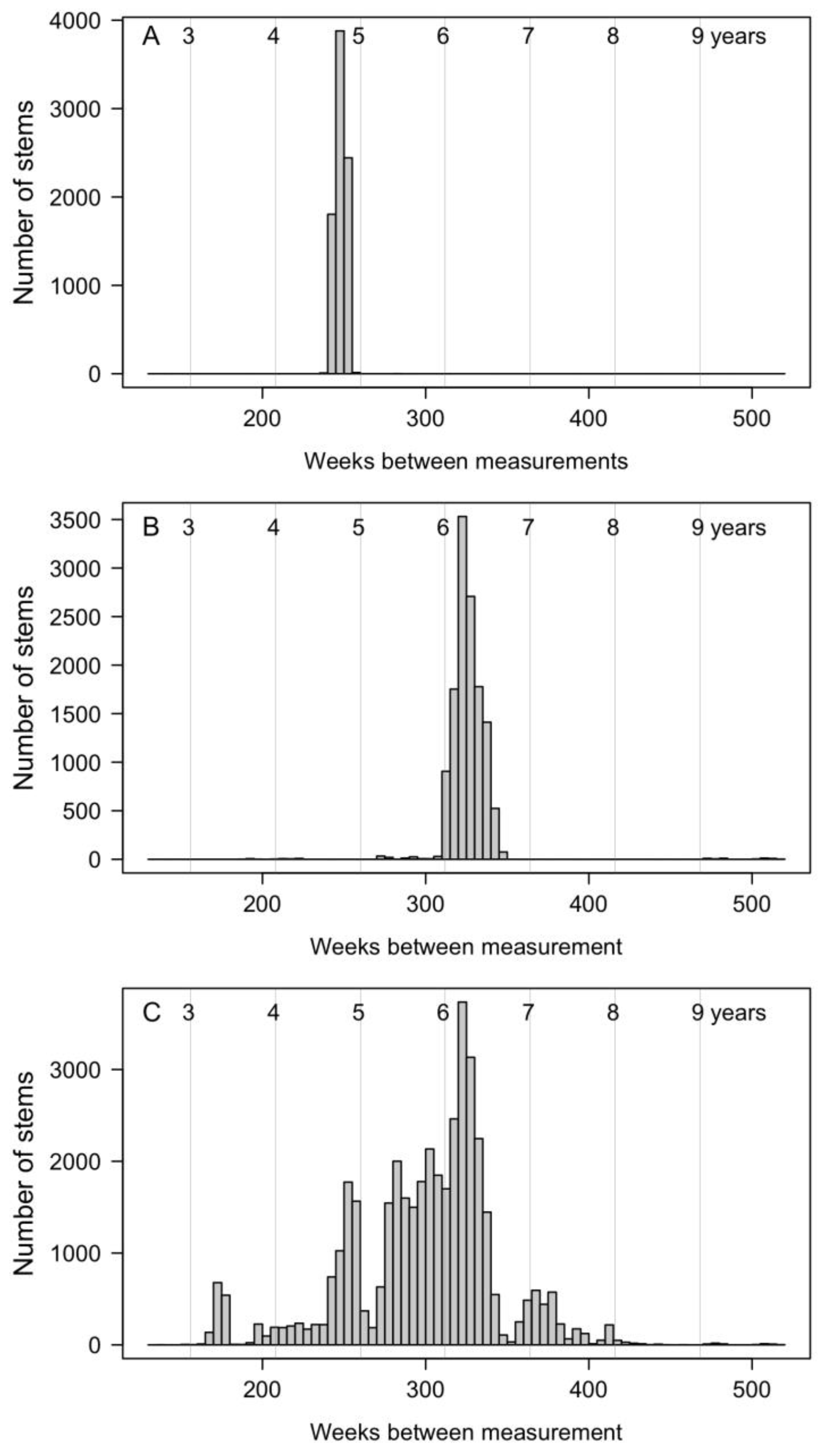
The UCSC FERP was established in 2007 as part of the CTFS/Forest Global Earth Observatory (ForestGEO; forestgeo.si.edu) network of sites for research on long-term forest dynamics and forest diseases, as well as to support experiential learning for UCSC students. The original 6 ha FERP was established with the help of graduate and undergraduate students and a technician, as acknowledged in the original publication on the FERP [31]. The expansion of the FERP to 16 ha and all subsequent data collection have been carried out almost entirely by undergraduate interns and student employees at UCSC, with organizational and field support by the authors and Campus Natural Reserve staff. Student interns receive academic credit for 6 h per week working on FERP censuses; the internship includes training in plant identification, measurement methods, field protocols, data entry, and the conceptual basis for the FERP. Students who excel during the internship are invited to become paid crew leaders in subsequent quarters. Crew leaders receive additional mentoring in field safety, leadership, and field research management and are responsible for training and leading groups of 4–10 interns in the forest. The first author (G.G.), who is the founding director of the UCSC FERP, has responsibility for data management and analysis, with support from author S.C. The last author (A.J.) has had primary responsibility for recruiting undergraduate interns and overseeing the crew leaders and trail maintenance, with A.K. providing additional support in those areas. We are grateful to all crew leaders and interns who participated in mapping and measuring woody plants on the expanded 16 ha FERP; their names are listed in Appendix C.

2.4. Census Periods

We report here data from three censuses, called FERP1, FERP2, and FERP3. The FERP1 census of the original 6 ha (previously reported in [31]) included the area from 0 to 200 m east and 0 to 300 m north. The FERP1 began on 8 December 2006 and ended on 13 September 2007. The FERP2 census began with the same 6 ha section, after which the extent of the UCSC FERP was expanded to its final 16 ha extent (0 to 400 m east and 0 to 400 m north). The FERP2 census began on 29 September 2011 and ended on 17 June 2015. The FERP3 census began on 5 August 2017 and ended on 29 November 2021. For both FERP2 and FERP3, the initial pass through the plot was followed by a period of revisiting stems throughout the plot for which original data were incomplete or questionable (e.g., an excessively dramatic change in DSH between censuses). That period of review is included in the census dates.

The intercensus intervals were then calculated as the number of days between measurements of the same stems, divided by 365 to put the interval value in units of years. The median intercensus interval from FERP1 to FERP2 (6 ha only) was 4.788 years (95% of all intervals were between 4.637 and 4.898 years). The median intercensus duration from FERP2 to FERP3 (all 16 ha) was 5.882 years (95% of all intervals were between 3.387 and 7.327 years). Including only stems in the original 6 ha area, the median intercensus duration from FERP2 to FERP3 (6 ha only) was 6.253 years (95% of all durations were between 6.022 and 6.574 years). Details of the distributions of intercensus intervals are shown in Appendix D (Figure A3).

2.5. Mortality Rates

Annual mortality rates were calculated for each intercensus interval based on the following equation:

$$\lambda =\frac{\ln \left(n_0\right)-\ln \left(n_{\mathrm{t}}\right)}{t},$$

(1)

where n₀ and n_t are the number of live stems in one census and that in the next census after t years. Because variation across the plot in the elapsed time (duration) between observations affects the accuracy of the annualized mortality rate [38], we provide an estimate of the error in annual mortality rates by using the median intercensus duration and the 0.025 and 0.975 quantile times (95% confidence interval).

2.6. Growth Rates

Absolute annual growth rates were calculated for each intercensus interval as the difference in diameter measurements from one census to the next, divided by the number of years between measurements of that stem, with units in mm yr⁻¹. The relative growth rate was calculated as RGR = (ln(DSH_t) − ln(DSH_t-1)/(time_t − time_t−1), with units in cm cm⁻¹ yr⁻¹ (or simply yr⁻¹) [39]. The growth rate was only calculated for stems alive at the beginning and end of the interval. The analysis included stems that grew as well as those that apparently decreased in size, either from seasonal shrinkage or from measurement error (e.g., not measured at exactly the same place). We did, however, exclude 40 stems from the analysis (stem 1 of tags 371, 577, 736, 1220, 1333, 1378, 1512, 1937, 2699, 3685, 3940, 4408, 4578, 4619, 4706, 5517, 6699, 6772, 7234, 7854, 12,231, 12,354, 12,872, 14,454, 16,482, 16,493, 17,631, 18,707, 20,864, 21,244, 21,605, 22,194, 22,433, 22,629, 24,216, 25,532, 26,605, 26,609, 26,750, 26,772) because they had biologically implausible changes in size from one census to another, likely due to recording errors. An additional 195 stems that had broken below 1.3 m but remained alive were removed from growth analyses.

2.7. Availability of Data

The full set of data from the three censuses is available on Dryad as a .csv flat file (https://doi.org/10.5061/dryad.6q573n64s). Additionally, the data are available on the ForestGEO web site at https://forestgeo.si.edu/explore-data/uc-santa-cruz-termsconditionsrequest-forms. Analytical code and associated files for species taxonomy and plot coordinates are available as Supplementary Materials, below.

3. Results

Here, we report the descriptive statistics of forest composition and structure for the first three censuses of the University of California Santa Cruz Forest Ecology Research Plot (FERP). The first census included 6 ha (FERP1, 2007). Beginning with the second census of those 6 ha (starting in 2011), the FERP was expanded to 16 ha (FERP2, 2011–2015). The full 16 ha was censused again for FERP3 (2017–2021). We report statistics for the original 6 ha area for each of the three censuses, as well as for the full 16 ha for FERP2 and FERP3. Across the three censuses, we report identity, size, mortality, and growth data from 48,556 stems of 31,206 mapped woody individuals of trees, shrubs, and lianas.

3.1. Species Composition

The woody vegetation on the UCSC FERP includes 34 species from 20 families (

Table 1. Woody species present on the UC Santa Cruz Forest Ecology Research Plot.

Scientific Name	Family	Common Name	Origin	Habit	Code 1
Acer macrophyllum Pursh	Sapindaceae	Bigleaf maple	Native	Tree	ACERMA
Adenostoma fasciculatum Hook. & Arn.	Rosaceae	Chamise	Native	Shrub	ADENFA
Arbutus menziesii Pursh	Ericaceae	Pacific madrone	Native	Tree	ARBUME
Arctostaphylos andersonii A. Gray	Ericaceae	Santa Cruz manzanita	Native	Shrub	ARCTAN
Arctostaphylos crustacea subsp. crinita (J.E.Adams) V.T.Parker, M.C.Vasey & J.E.Keeley	Ericaceae	Brittle leaf manzanita	Native	Shrub	ARCTCR
Baccharis pilularis DC.	Asteraceae	Coyote brush	Native	Shrub	BACCPI
Ceanothus thyrsiflorus Eschsch.	Rhamnaceae	Blueblossom	Native	Shrub	CEANTH
Corylus cornuta subsp. californica Marshall (A.DC.) A.E.Murray	Betulaceae	Beaked hazelnut	Native	Shrub	CORYCO
Cotoneaster franchetii Bois	Rosaceae	Franchet cotoneaster	Intro	Shrub	COTOFR
Cotoneaster pannosus Franch.	Rosaceae	Woolly cotoneaster	Intro	Shrub	COTOPA
Crataegus monogyna Jacq.	Rosaceae	One-seed hawthorn	Intro	Shrub	CRATMO
Eriobotrya japonica (Thunb.) Lindl.	Rosaceae	Loquat	Intro	Tree	ERIOJA
Eucalyptus globulus Labill.	Myrtaceae	Blue gum	Intro	Tree	EUCAGL
Frangula californica (Eschsch.) A.Gray	Rhamnaceae	California coffeeberry	Native	Shrub	RHAMCA
Hedera helix L.	Araliaceae	English ivy	Intro	Liana	HEDEHE
Heteromeles arbutifolia (Lindl.) M.Roem	Rosaceae	Toyon	Native	Shrub	HETEAR
Ilex aquifolium L.	Aquifoliaceae	English holly	Intro	Tree	ILEXAQ
Lonicera hispidula (Lindl.) Douglas ex Torr. & A.Gray	Caprifoliaceae	Pink honeysuckle	Native	Liana	LONIHI
Morella californica (Cham.) Wilbur	Myricaceae	California wax myrtle	Native	Shrub	MORECA
Notholithocarpus densiflorus (Hook. & Arn.) Manos, C.H. Cannon & S.H.Oh	Fagaceae	Tanoak	Native	Tree	LITHDE
Pinus attenuata Lemmon	Pinaceae	Knobcone pine	Native	Tree	PINUAT
Pinus ponderosa var. pacifica J.R.Haller & Vivrette	Pinaceae	Pacific ponderosa pine	Native	Tree	PINUPO
Pseudotsuga menziesii (Mirb.) Franco	Pinaceae	Douglas fir	Native	Tree	PSEUME
Pyracantha angustifolia C.K.Schneid	Rosaceae	Firethorn	Intro	Shrub	PYRAAN
Quercus agrifolia Née	Fagaceae	Coast live oak	Native	Tree	QUERAG
Quercus parvula var. shrevei (C.H.Mull.) Nixon	Fagaceae	Shreve’s oak	Native	Tree	QUERPA
Rhododendron occidentale (Torr. & A.Gray) A.Gray	Ericaceae	Western azalea	Native	Shrub	RHODOC
Ribes divaricatum Douglas	Grossulariaceae	Spreading gooseberry	Native	Shrub	RIBEDI
Salix lasiandra Benth.	Salicaceae	Pacific willow	Native	Shrub	SALILA
Sambucus caerulea Raf.	Vibernaceae	Blue elderberry	Native	Shrub	SAMBNI
Sequoia sempervirens (D.Don) Endl.	Cupressaceae	Coast redwood	Native	Tree	SEQUSE
Toxicodendron diversilobum Greene	Anacardiaceae	Poison oak	Native	Liana	TOXIDI
Umbellularia californica (Hook. & Arn.) Nutt.	Lauraceae	California bay	Native	Tree	UMBECA
Vaccinium ovatum Pursh	Ericaceae	Evergreen huckleberry	Native	Shrub	VACCOV

¹ Name changes since Gilbert et al. (2010) [31] include ARCTCR (from A. tomentosa subsp. crustaceae), LITHDE (from Lithocarpus densiflorus), RHAMCA (from Rhamnus californica), and SAMBNI (from S. nigra subsp. caerulea). Original codes are retained for continuity. The family of SAMBNI changed from Caprifoliaceae to Vibernaceae.

). This includes 4 species of gymnosperm trees, 9 species of angiosperm trees, 18 species of shrubs, and 3 species of lianas (woody vines). The overall composition of the forest remained stable across the three censuses.

3.2. Abundance and Basal Area

The average densities of individuals, stems, and basal area for three censuses of the FERP are summarized in

Table 2. Average densities of individuals, stems, and basal area across the UC Santa Cruz FERP in three censuses. Values for 6 ha include the area of the original FERP1 census only; values for 16 ha represent the entire area of the 16 ha FERP. Adjusted densities (adj) are calculated for an area of 15.939 ha, adjusting for the 614 m² occupied by the fire road (Chinquapin Road), where vegetation is not permitted to grow.

	6 ha				16 ha
Density Measure	FERP1	FERP2	FERP3		FERP2	FERP3
Individuals ha−1	1363.3	1378.7	1158.2		1630.2	1558.7
Stems ha−1	1941.0	1992.3	1724.0		2488.8	2303.1
Basal area m2 ha−1	47.2	49.1	48.6		66.9	68.3
Individuals ha−1 (adj)	-	-	-		1636.4	1564.7
Stems ha−1 (adj)	-	-	-		2498.3	2311.9
Basal area m2 ha−1 (adj)	-	-	-		67.2	68.6

both for the entire 16 ha (FERP2 and FERP3) and for just the 6 ha extent of the original FERP1 census. From FERP2 to FERP3, there was a 4.4% reduction in the number of individuals and a 7.5% reduction in the number of stems but a 2.0% increase in basal area, reflecting a process of self-thinning in the forest and the continued growth of survivors.

The forest vegetation is dominated by native species but includes eight non-native (introduced) invasive species, including five in the Rosaceae family, Eucalyptus globulus (Blue gum, Myrtaceae), Hedera helix (English Ivy, Araliaceae), and Ilex aquifolium (English holly, Aquifoliaceae) (Table 1). Invasive species together make up 0.39% of the individuals, 0.49% of the stems, and 0.04% of the basal area on the FERP (Table 1 and

Table 3. Number of individuals of each woody species on the UC Santa Cruz Forest Ecology Research Plot in each of the three censuses. Species codes are given in Table 1. Values for 6 ha show the number of individuals within the 6 ha region of the original FERP1 census.

	6 ha				16 ha
Code	FERP1	FERP2	FERP3		FERP2	FERP3
ACERMA	2	2	2		10	9
ADENFA	0	0	0		1	0
ARBUME	687	597	305		845	415
ARCTAN	11	7	1		9	11
ARCTCR	39	23	11		28	13
BACCPI	11	1	1		6	14
CEANTH	1	1	0		2	2
CORYCO	146	146	155		478	477
COTOFR	18	21	17		22	19
COTOPA	36	32	33		35	38
CRATMO	1	1	1		1	1
ERIOJA	0	0	0		1	1
EUCAGL	5	5	5		6	6
HEDEHE	8	7	12		11	16
HETEAR	11	8	11		52	50
ILEXAQ	10	9	11		13	16
LITHDE	1260	1630	1504		6164	6314
LONIHI	217	197	126		490	318
MORECA	8	8	3		52	39
PINUAT	1	0	0		3	3
PINUPO	17	10	7		15	13
PSEUME	2158	2121	1864		8005	7308
PYRAAN	1	1	1		1	1
QUERAG	908	856	749		1242	1159
QUERPA	1196	1202	1192		3860	4747
RHAMCA	293	268	148		388	236
RHODOC	0	0	0		215	150
RIBEDI	1	1	0		3	3
SALILA	2	2	2		4	4
SAMBNI	2	2	1		3	3
SEQUSE	190	194	196		2001	2015
TOXIDI	675	638	341		1229	732
UMBECA	11	11	10		16	14
VACCOV	254	271	240		872	792
Total	8180	8272	6949		26,083	24,939

,

Table 4. Number of stems of each woody species on the UC Santa Cruz Forest Ecology Research Plot in each of the three censuses. Species codes are given in Table 1. Values for 6 ha show the number of individuals within the 6 ha region of the original FERP1 census.

	6 ha				16 ha
Code	FERP1	FERP2	FERP3		FERP2	FERP3
ACERMA	3	2	2		12	9
ADENFA	0	0	0		1	0
ARBUME	907	742	409		1060	556
ARCTAN	24	9	1		14	32
ARCTCR	74	46	15		54	19
BACCPI	24	1	1		27	40
CEANTH	1	1	0		2	3
CORYCO	874	920	1092		3231	3016
COTOFR	57	59	42		60	44
COTOPA	71	65	76		71	81
CRATMO	1	1	1		1	1
ERIOJA	0	0	0		1	1
EUCAGL	5	6	6		8	8
HEDEHE	8	7	13		11	17
HETEAR	36	23	27		160	135
ILEXAQ	21	14	20		25	27
LITHDE	1566	2313	2099		9675	9297
LONIHI	228	217	136		534	344
MORECA	12	9	5		108	70
PINUAT	1	0	0		3	3
PINUPO	17	10	7		15	13
PSEUME	2207	2176	1929		8339	7592
PYRAAN	1	2	2		2	2
QUERAG	1061	1007	874		1500	1385
QUERPA	1678	1694	1680		5728	6776
RHAMCA	464	470	258		744	449
RHODOC	0	0	0		629	452
RIBEDI	3	1	0		3	3
SALILA	3	3	4		8	9
SAMBNI	2	2	1		4	9
SEQUSE	238	263	258		3046	2924
TOXIDI	726	709	380		1362	802
UMBECA	13	13	13		18	17
VACCOV	1320	1169	993		3365	2713
Total	11,646	11,954	10,344		39,821	36,849

and

Table 5. Basal area (m²) of each woody species on the UC Santa Cruz Forest Ecology Research Plot in each of the three censuses. Species codes are given in Table 1. Values for 6 ha show the number of individuals within the 6 ha region of the original FERP1 census.

	6 ha				16 ha
Code	FERP1	FERP2	FERP3		FERP2	FERP3
ACERMA	0.38097	0.46521	0.53047		1.46086	1.5160
ADENFA	0	0	0		0.00010	0
ARBUME	67.04084	59.66385	39.75019		94.86421	57.87346
ARCTAN	0.11528	0.04846	0.00018		0.05267	0.01887
ARCTCR	0.20206	0.14434	0.05949		0.15199	0.06171
BACCPI	0.00814	0.00023	0.00038		0.00549	0.01935
CEANTH	0.02324	0.03048	0		0.03079	0.00106
CORYCO	0.29372	0.30811	0.41493		1.04925	1.22132
COTOFR	0.02203	0.02321	0.026		0.02336	0.02706
COTOPA	0.09969	0.13451	0.16585		0.13604	0.16802
CRATMO	0.00166	0.00173	0.00166		0.00173	0.00166
ERIOJA	0	0	0		0.00013	0.00008
EUCAGL	0.0244	0.08458	0.16591		0.08512	0.16724
HEDEHE	0.00616	0.01061	0.02279		0.01144	0.02424
HETEAR	0.09899	0.08072	0.08109		0.21873	0.20313
ILEXAQ	0.03951	0.04201	0.06493		0.05557	0.06836
LITHDE	9.39694	10.53444	10.39026		41.39863	36.90206
LONIHI	0.05187	0.06133	0.05087		0.13584	0.10142
MORECA	0.03905	0.02948	0.01946		0.10048	0.06096
PINUAT	0.03079	0	0		0.29882	0.31127
PINUPO	1.00556	1.49778	1.366		3.04374	3.15685
PSEUME	132.73041	150.37244	166.0646		332.96542	357.46774
PYRAAN	0.00057	0.00073	0.00076		0.00073	0.00076
QUERAG	32.69696	30.07165	26.66856		36.19849	32.61653
QUERPA	17.3345	14.04387	14.49981		34.71857	35.77295
RHAMCA	0.29838	0.41742	0.33405		0.68199	0.52023
RHODOC	0	0	0		0.14524	0.12705
RIBEDI	0.00072	0.00008	0		0.00024	0.00032
SALILA	0.01681	0.05385	0.10789		0.15586	0.18607
SAMBNI	0.00244	0.00343	0.00126		0.00714	0.00652
SEQUSE	20.55343	26.16681	30.32737		521.86279	563.20891
TOXIDI	0.12645	0.13451	0.11196		0.23866	0.19235
UMBECA	0.01869	0.01921	0.03316		0.08226	0.07376
VACCOV	0.32824	0.29923	0.36747		0.84534	0.87761
Total	282.9885	294.7443	291.6273		1071.0280	1092.9550

, FERP3 census).

There are obvious patterns of spatial variation in the woody plant density across the FERP. First, a visual inspection of the map of all individuals shows a clear gap in vegetation caused by Chinquapin Road (a dirt fire road) that crosses the northeastern corner of the FERP (Figure 2a). The road includes a total surface area of 614 m² where woody vegetation is not permitted to grow (0.38% of the FERP area). Average density calculations adjusted for this anthropogenically unavailable area are included in Table 2. The FERP2 and FERP3 maps (Figure 2a) also show a small (450 m²) extension of a natural meadow with a very low woody stem density at the northwestern corner of the FERP. At the northern end of the plot, just to the west of Chinquapin Road, is an area of noticeably high stem density (Figure 2a–c), primarily consisting of small-diameter Douglas-fir saplings. This stand appears to be from a major recruitment event of Douglas-fir seedlings following a massive multi-species canopy dieback event of unknown cause in 2004 that covered approximately 0.6 ha; this event is visible in historical imagery on Google Earth (Figure A4). Based on those images, the spatial extent of the mortality was visibly stable through at least 2006; from 2008 to 2010, the canopy mortality then extended westward to include an additional ~0.6 ha (Figure A4). At the time of the FERP2 census, that second mortality region had very little live woody vegetation amidst a graveyard of dead standing and fallen trees, as is apparent in a low-density area of the FERP2 map (Figure 2). Woody plants had begun to grow back into this area by FERP3.

The local densities of individuals (Figure 3a), stems (Figure 3b), and basal area (Figure 3c) are all right-skewed. The median densities of individuals for FERP1, FERP2, and FERP3 were 1250, 1400, and 1325 individuals ha⁻¹ (50, 56, and 53 individuals per quadrat). For stem density, the median values for the three censuses were 1775, 2200, and 2087 stems ha⁻¹ (71, 88, and 83 stems per 20 m × 20 m quadrat). The median basal area was 42.99, 51.60, and 52.75 m² ha⁻¹ for the three censuses. FERP1 values are based on just the 150 quadrats in the southwest part of the FERP, whereas FERP2 and FERP3 are for the entire 400 quadrats.

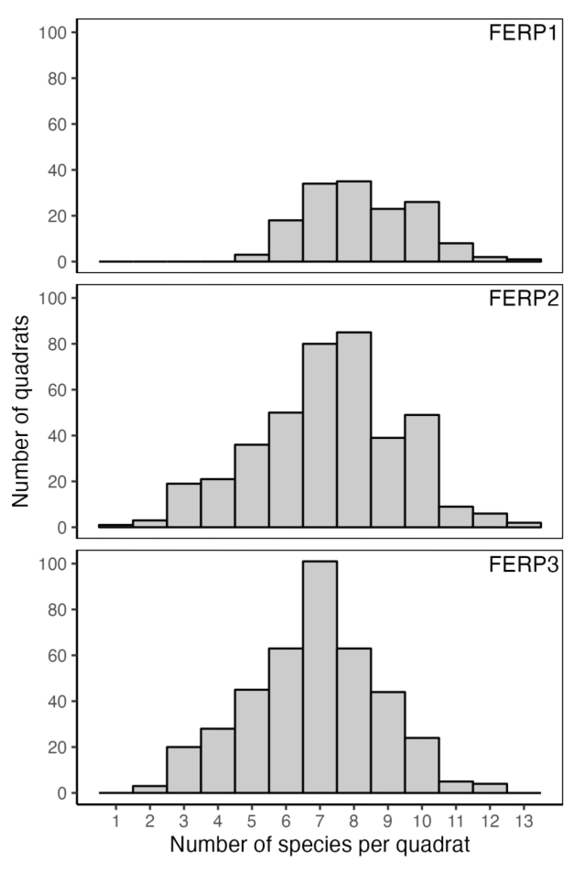
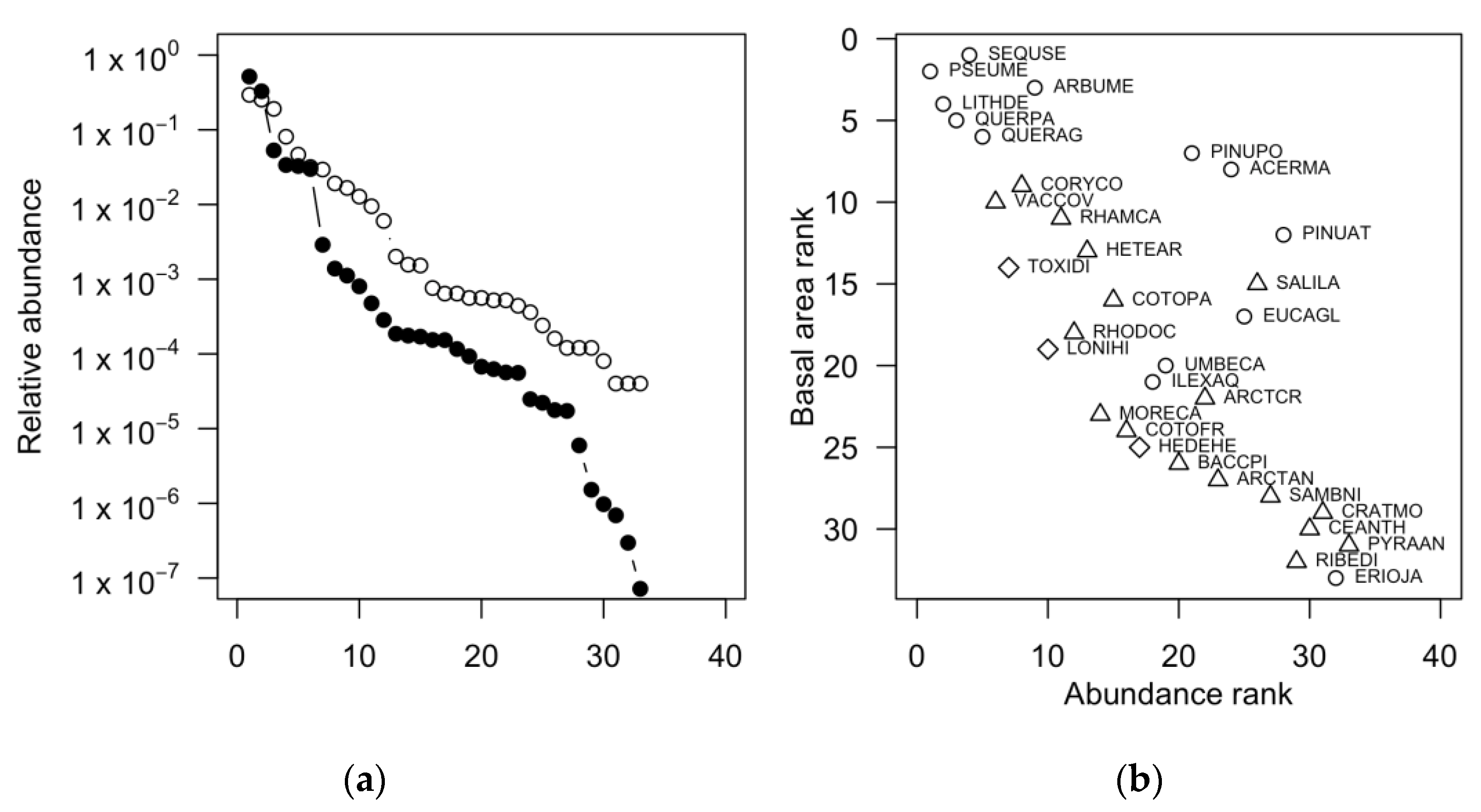
3.3. Community Structure and Species Relative Abundance

There was no statistically significant relationship between the number of individuals and the total basal area within quadrats across all species (Figure 4a). A high basal area density is associated with a few large-diameter trees, rather than a large number of stems; in contrast, species richness increased significantly with the increasing number of individuals in a quadrat (Figure 4b) and decreased with increasing basal area (Figure 4c), although both with poor fits. The effect of abundance on species richness was better described with an additive combination of number of individuals and basal area (Number of species = 3.8959 + 2.1498 × log₁₀(number of individuals) − 0.0115 × basal area, R² = 0.20, F_2,397 = 49.7, p ≤ 2.2 × 10⁻¹⁶; the interaction term was not significant).

As with most biological communities, the FERP woody vegetation has a few species that are very common and a larger number of species that are much less abundant (Table 3, Table 4 and Table 5). Rank–abundance plots (Figure 5a) show that the distinction between common and less common species is more abrupt when measured as a function of the basal area than as the number of individuals. The rank order of species differs depending on which measure of abundance is used (Figure 5b). However, six tree species—Pseudotsuga menziesii (Douglas-fir), Sequoia sempervirens (coast redwood), Notholithocarpus densiflorus (tanoak), Quercus agrifolia (coast live oak), Quercus parvula var. shrevei (Shreve’s oak), and Arbutus menziesii (Pacific madrone)—stand out as the top-ranked species for both the number and basal area (Figure 5b). Together, they make up 88.0% of all individuals (99.7% of all tree individuals), 77.4% of all stems (99.7% of all tree stems), and 99.2% of all basal area (99.5% of tree basal area) on the FERP (Table 3, Table 4 and Table 5, FERP3).

The 18 species of shrub constitute 19.2% of all the stems on the FERP but only 7.4% of the individuals and 0.3% of the basal area (Table 1 and Table 3, Table 4 adnd Table 5, FERP3). The three species of liana represent 3.2% of the stems, 4.3% of the individuals, and just 0.03% of the basal area (Table 1, Table 2, Table 3 and Table 4, FERP3).

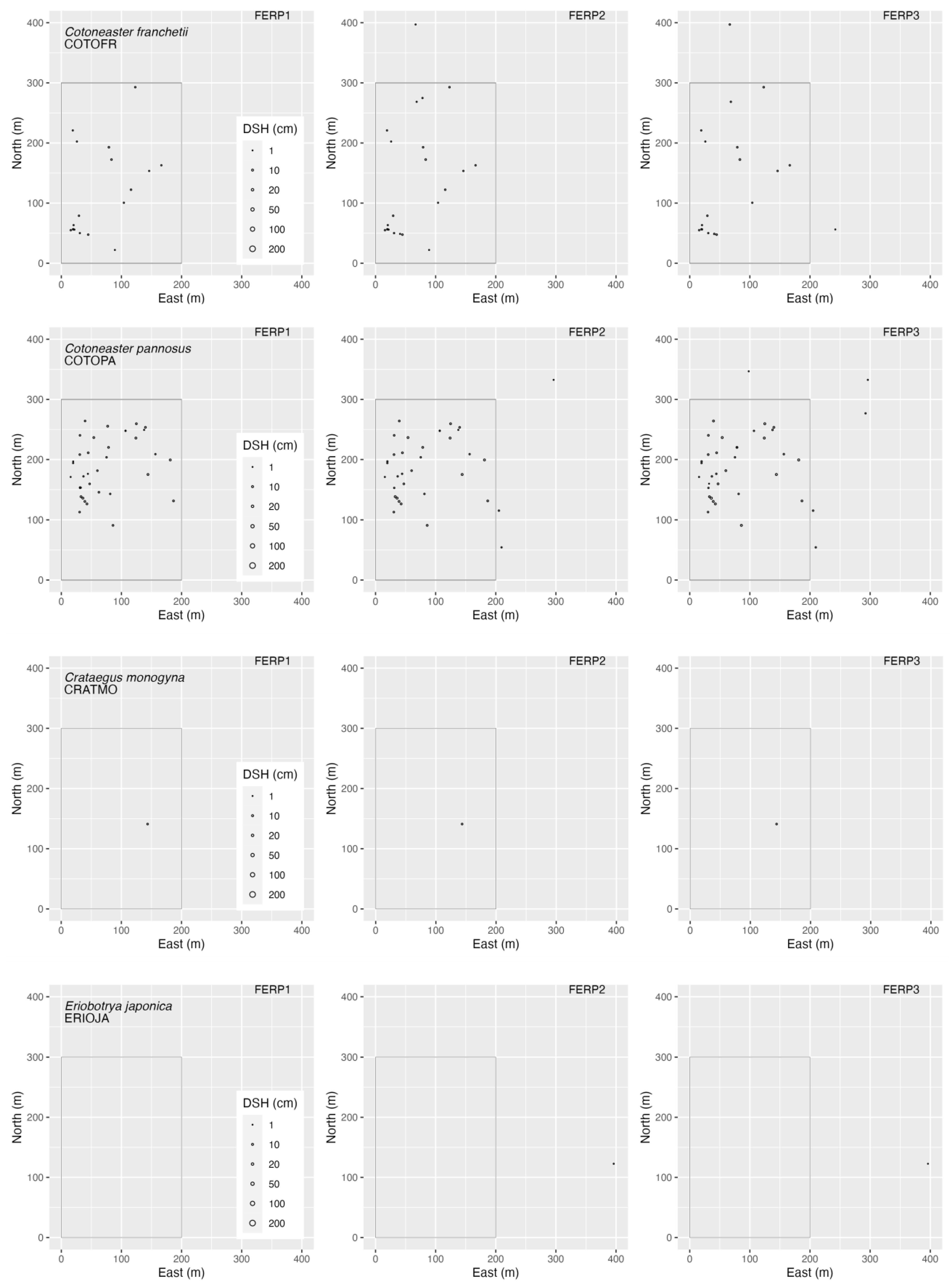
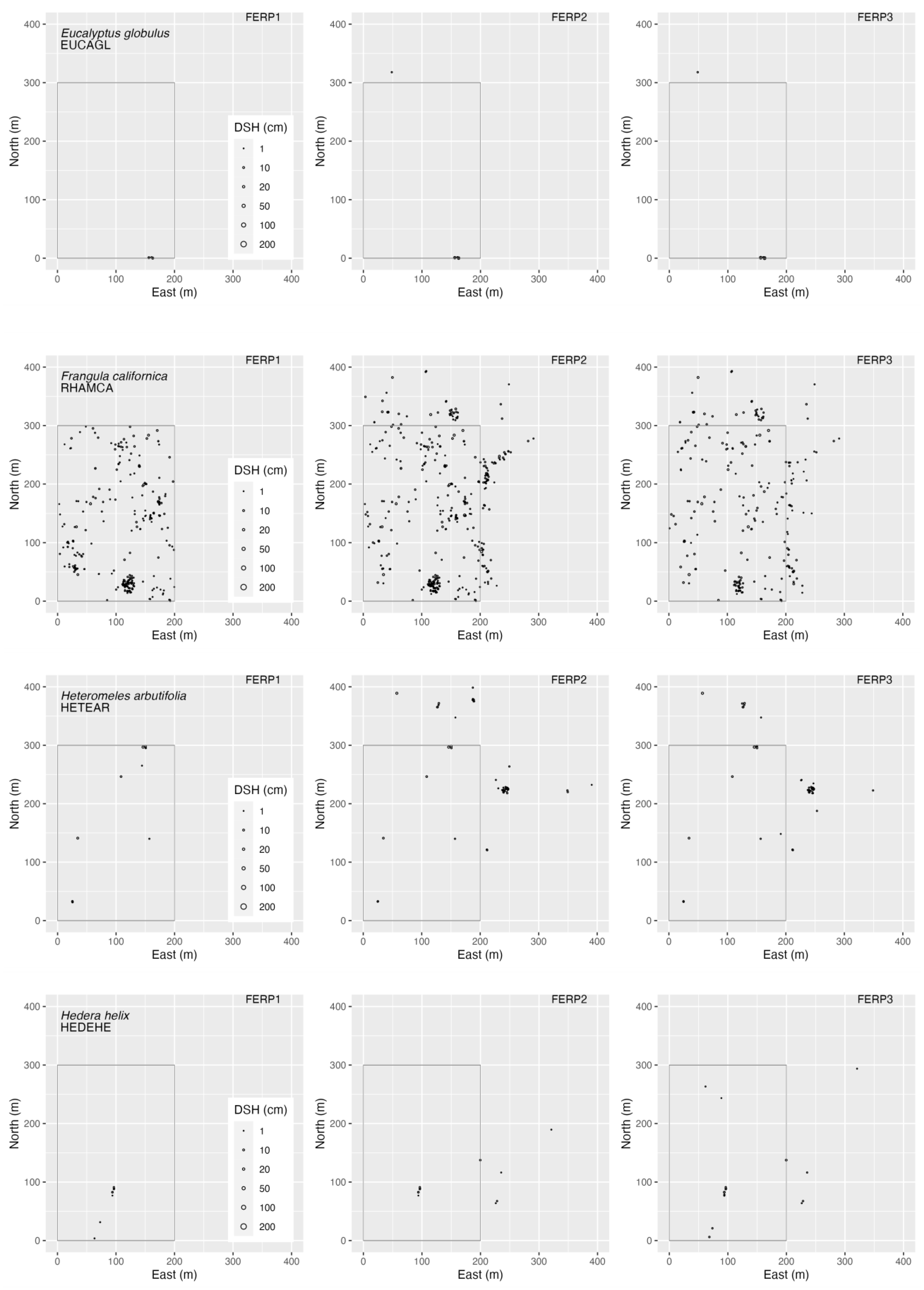
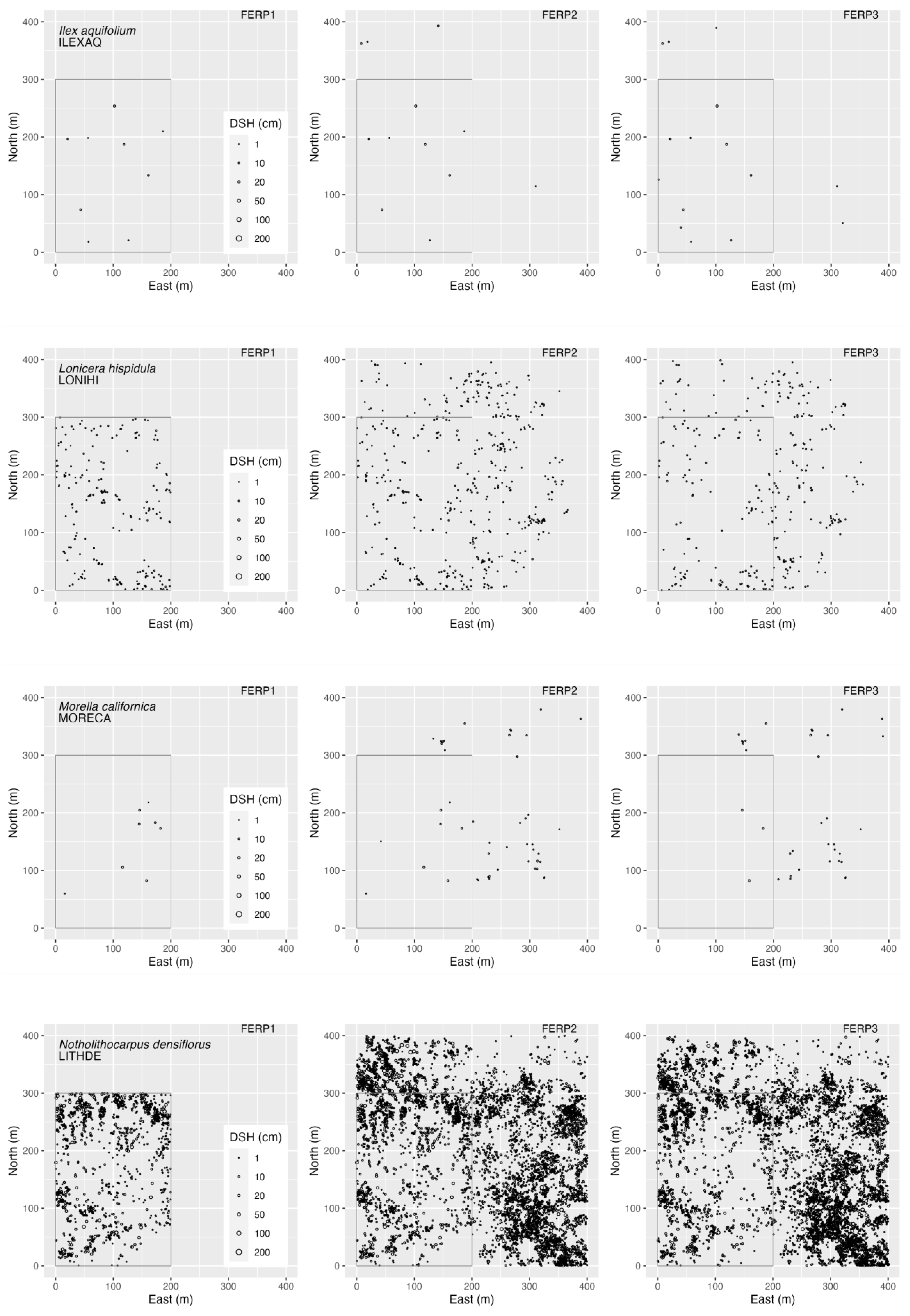
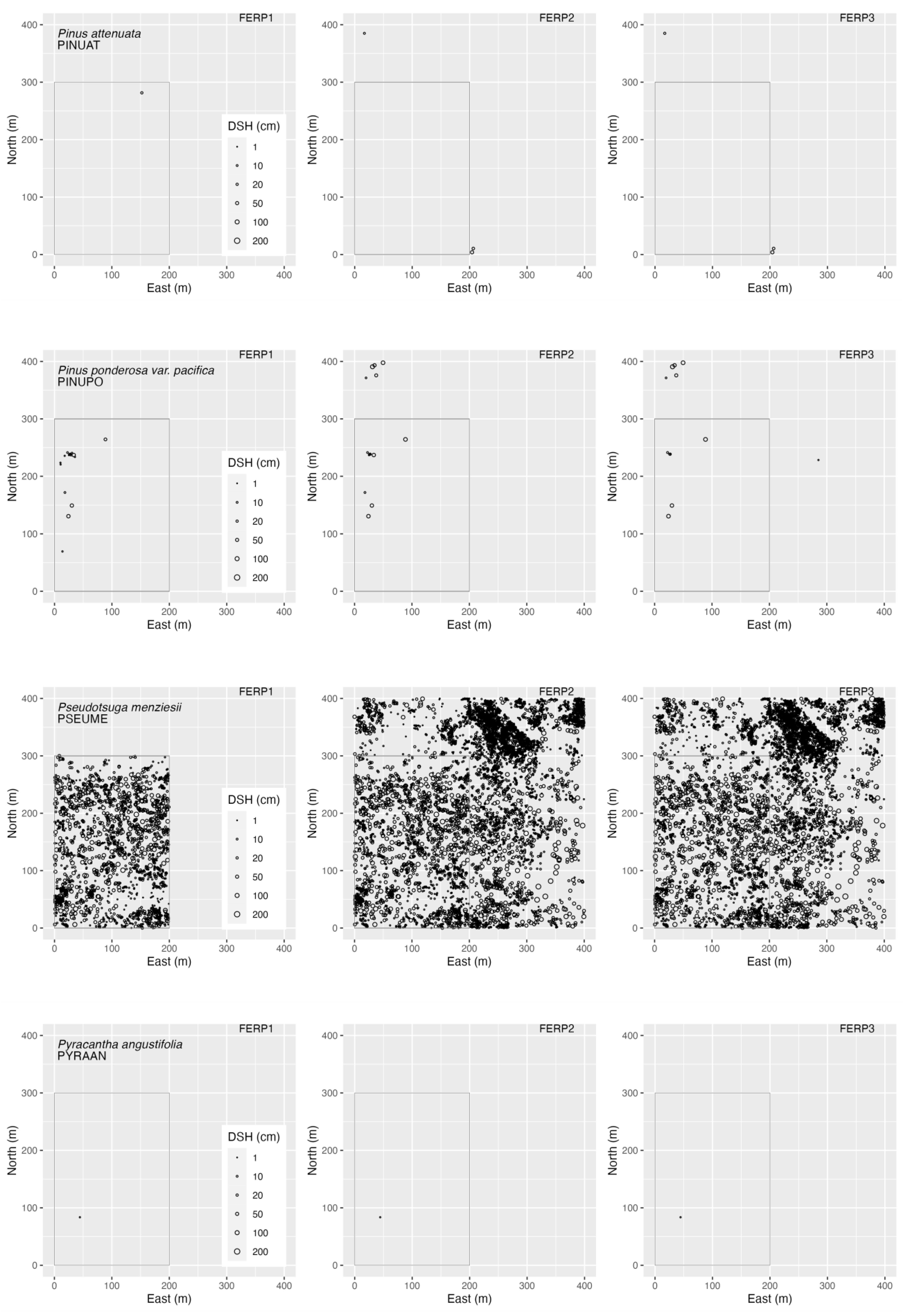
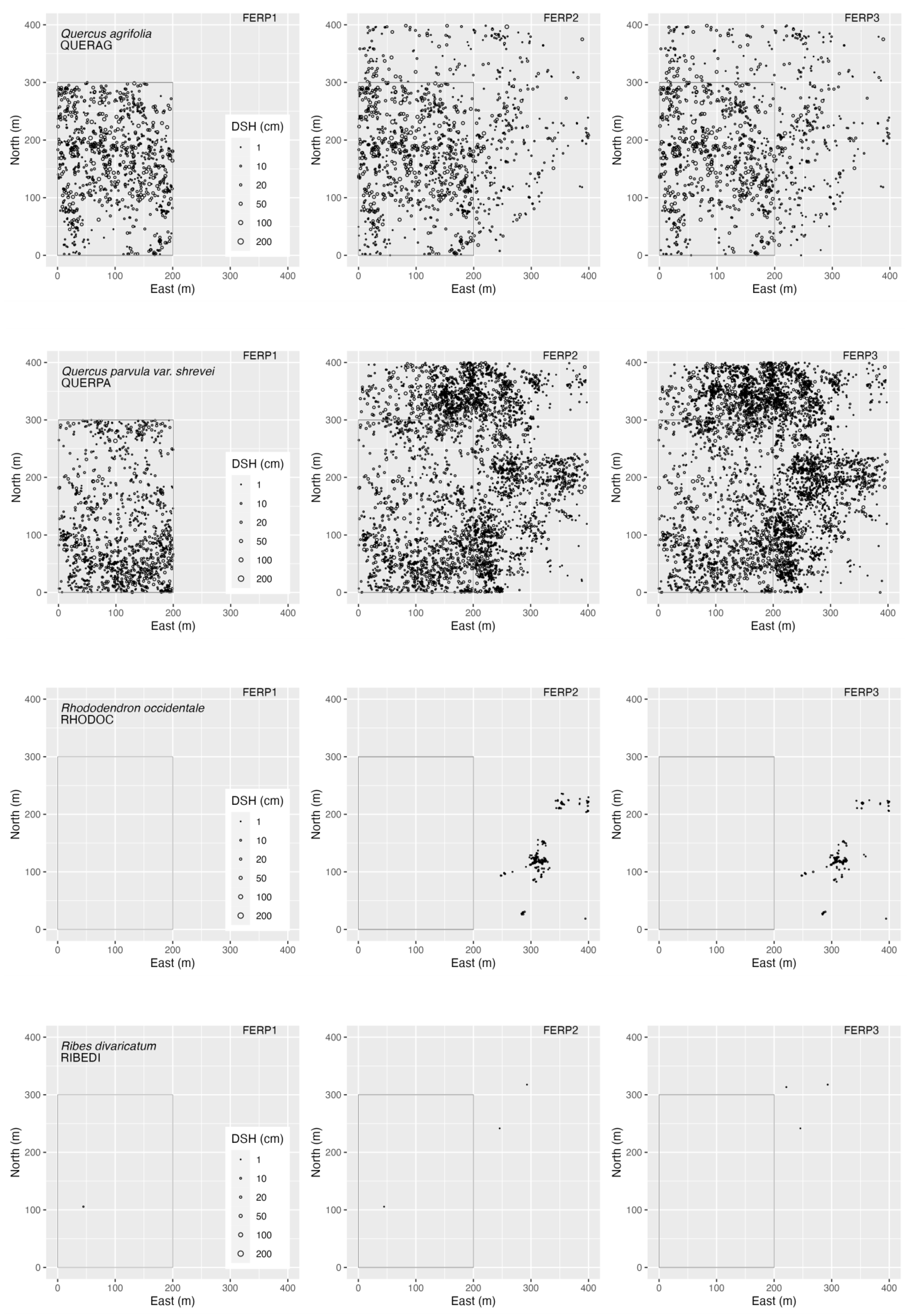
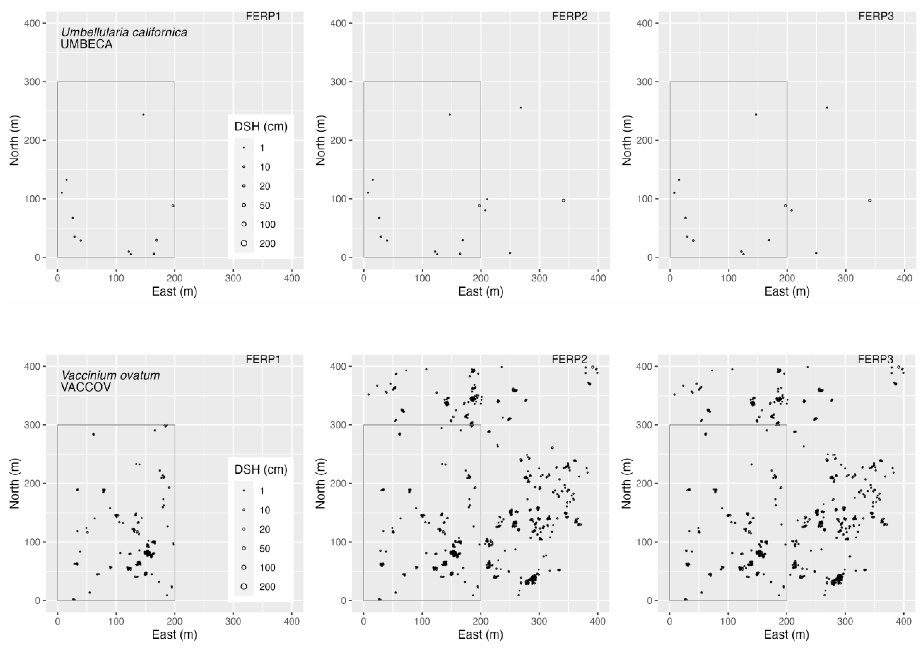
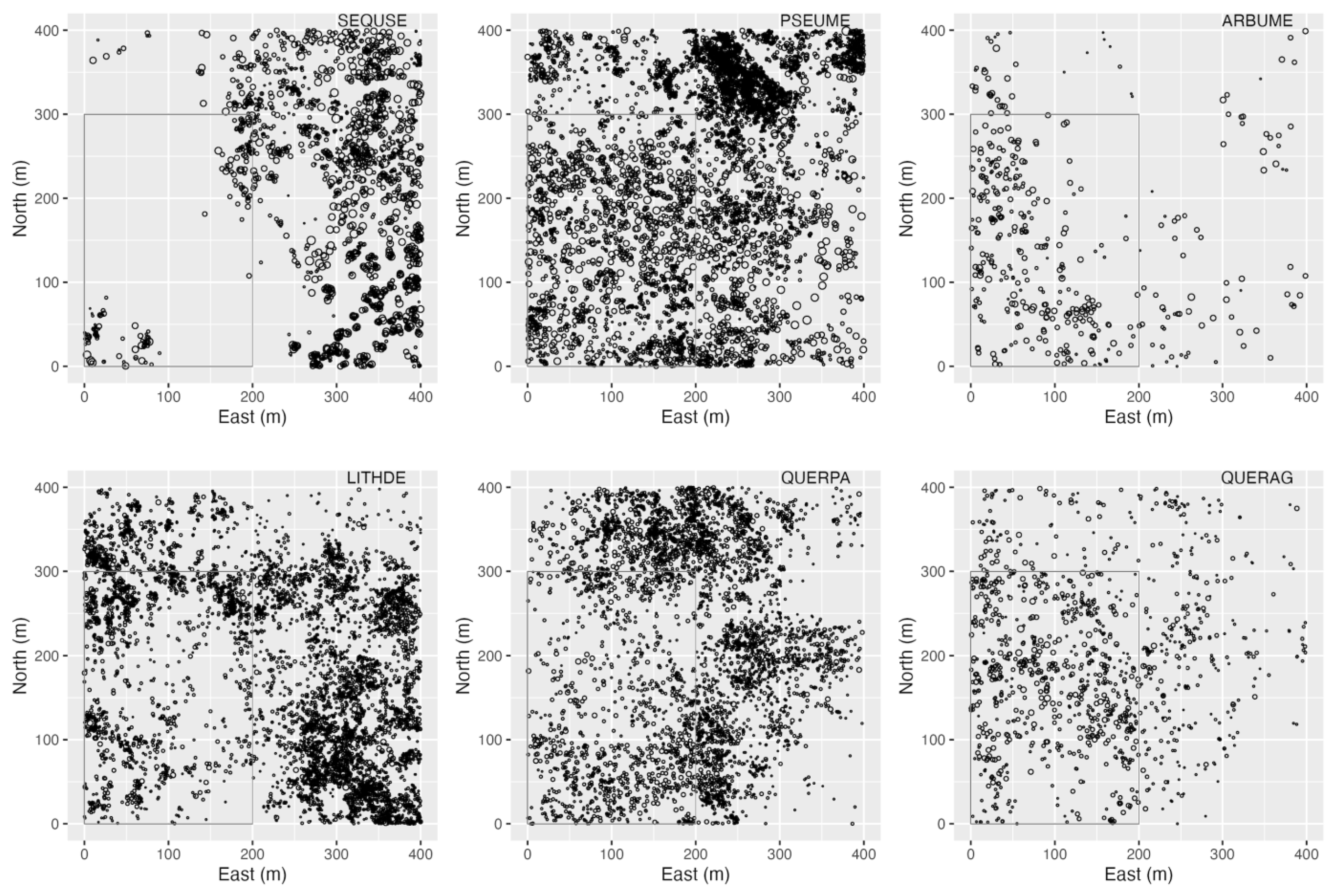
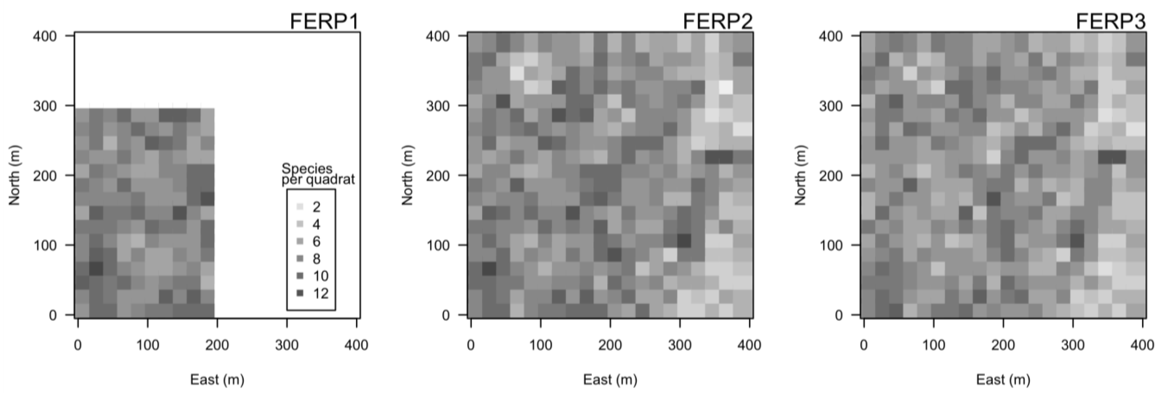
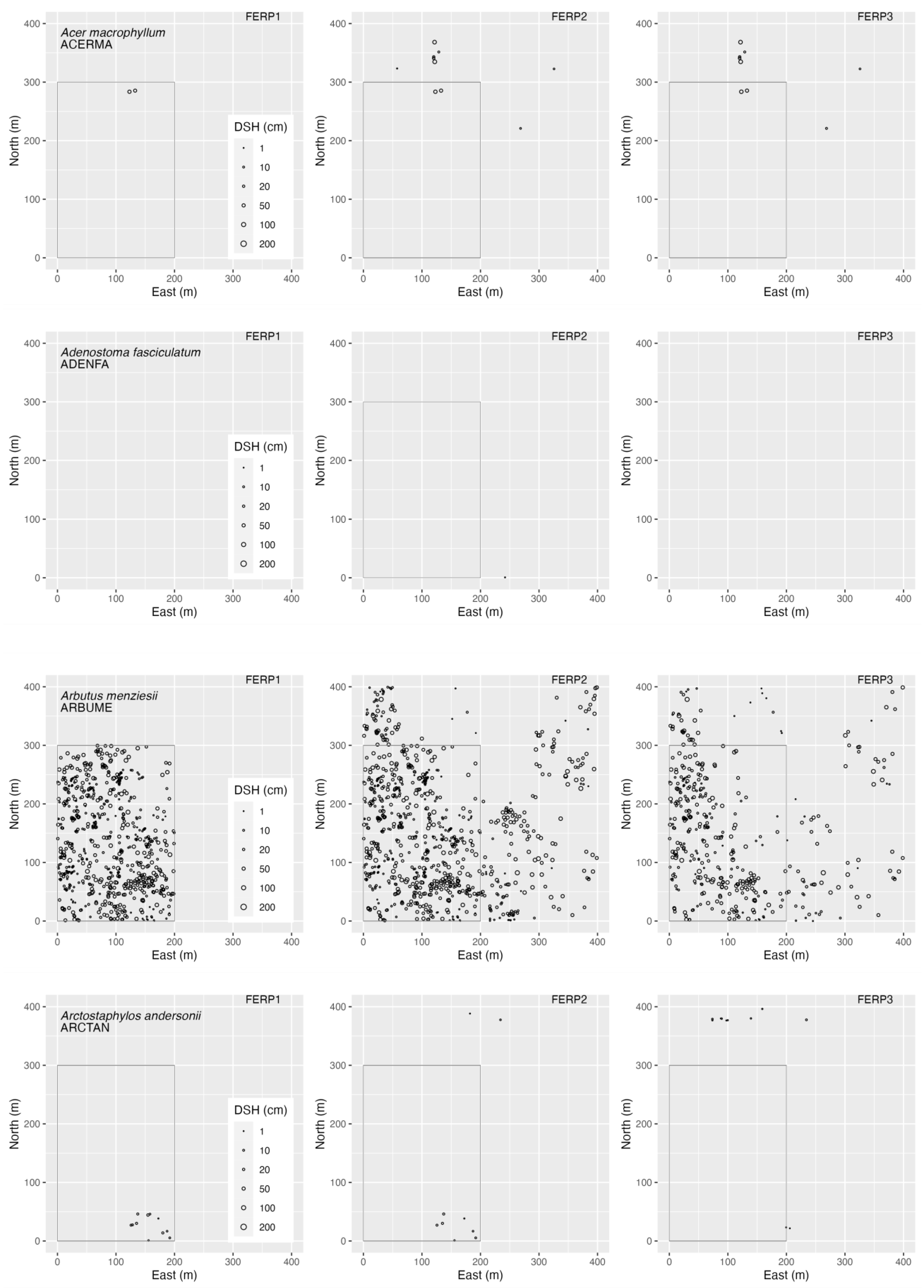
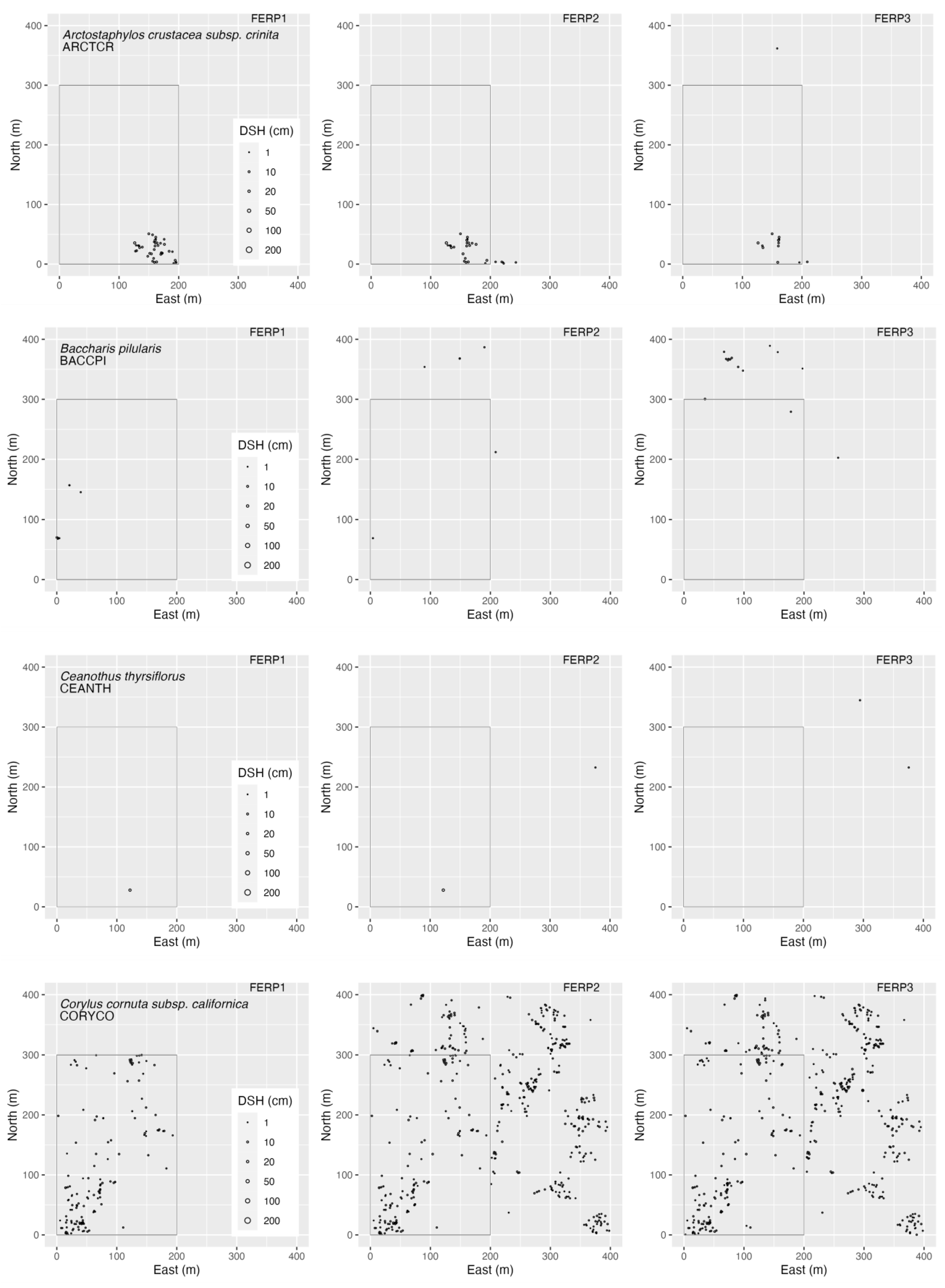
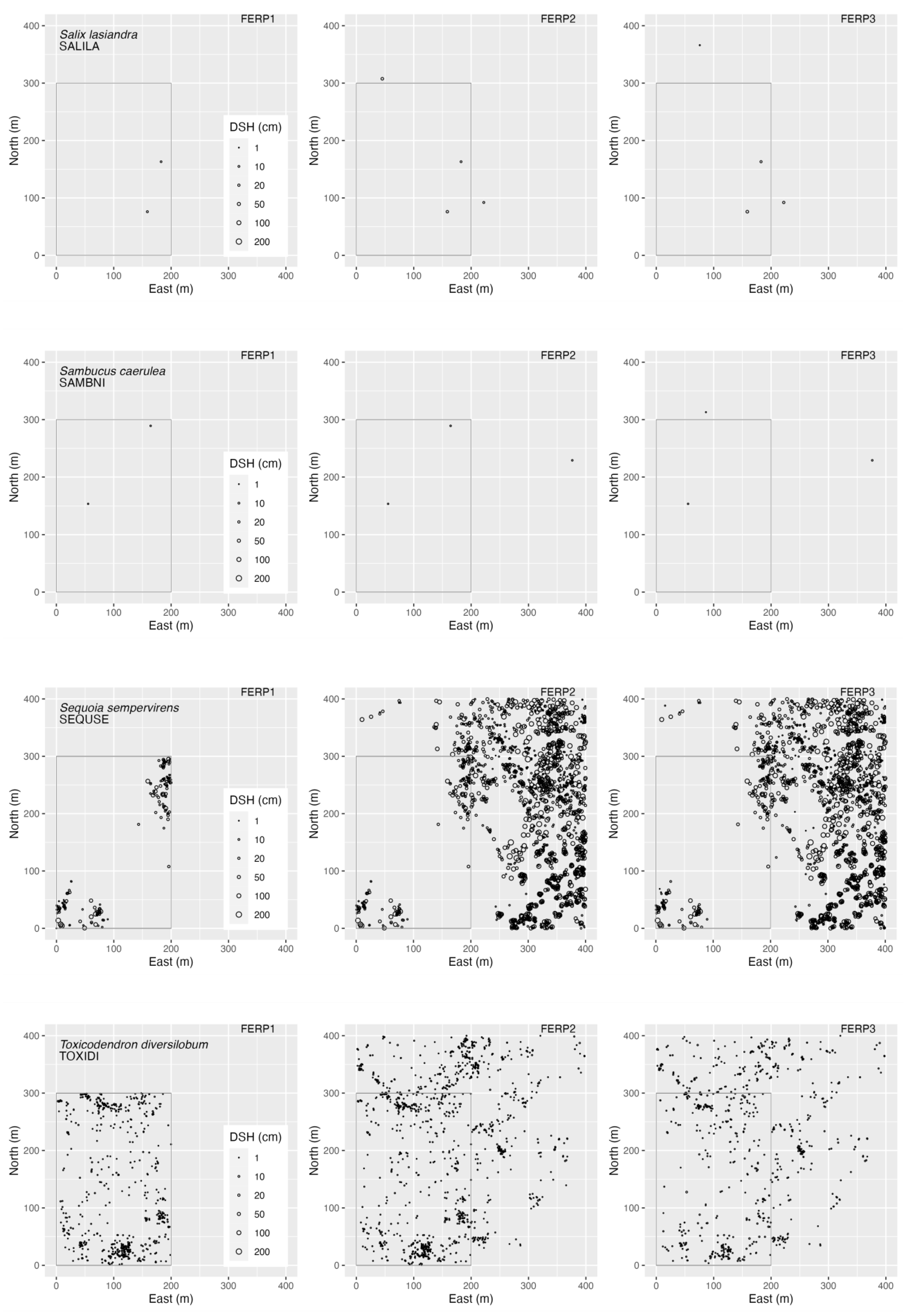
3.4. Spatial Patterns

The six most abundant species of trees (99% of basal area, Figure 5b) represent the dominant structure of the forest, and they have distinctive spatial patterns (Figure 6). The western half is a mixed-evergreen forest comprising a mix of the three oak species (Fagaceae: Quercus parvula, Q. agrifolia, and Notholithocarpus densiflorus), Douglas-fir (Pseudotsuga menziesii, Pinaceae), and Pacific madrone (Arbutus menziesii, Ericaceae). The eastern half is dominated by coastal redwood (Sequoia sempervirens, Cupressaceae), together with Douglas-fir and tanoak (Notholithocarpus). The three species of Fagaceae have notably complementary spatial patterns in the forest (Figure 6). Maps of each individual species, provided separately for FERP1, FERP2, and FERP 3 censuses, are presented in Appendix F (Figure A5).

A few less common species show noteworthy spatial patterns reflective of obvious history or habitat characteristics (Figure A5). The two manzanita species (Arctostaphylos andersonii and A. crustacea subsp. crinita) and most individuals of Pinus attenuata are limited to a small area in the south-central part of the FERP as remnants of the northern extent of the high-light-requiring chaparral community that has been taken over (shaded out) by the growth of tall Douglas-fir. Just to the west are Eucalyptus globulus, presumed offspring of large individuals that had been planted along an entrance road to the Cave Gulch community, south of the FERP. Rhododendron occidentale, the western azalea, is found only in areas with very wet soils and seeps associated with the stream drainage in the southeast corner.

Species richness varies across the FERP (Figure 7), with an average of seven woody species per 20 m × 20 m quadrat (range 2 to 12; FERP1: median = 8 (mean ± st.dev. 8.22 ± 1.60); FERP2: 7 (7.27 ± 2.13); FERP3 7 (6.83 ± 1.95)) (Figure A6). Diversity is lowest in the easternmost 100 m of the plot in areas that are dominated by large-diameter Sequoia sempervirens and Pseudotsuga menziesii, with a dense subcanopy of smaller Notholithocarpus densiflorus (Figure 6).

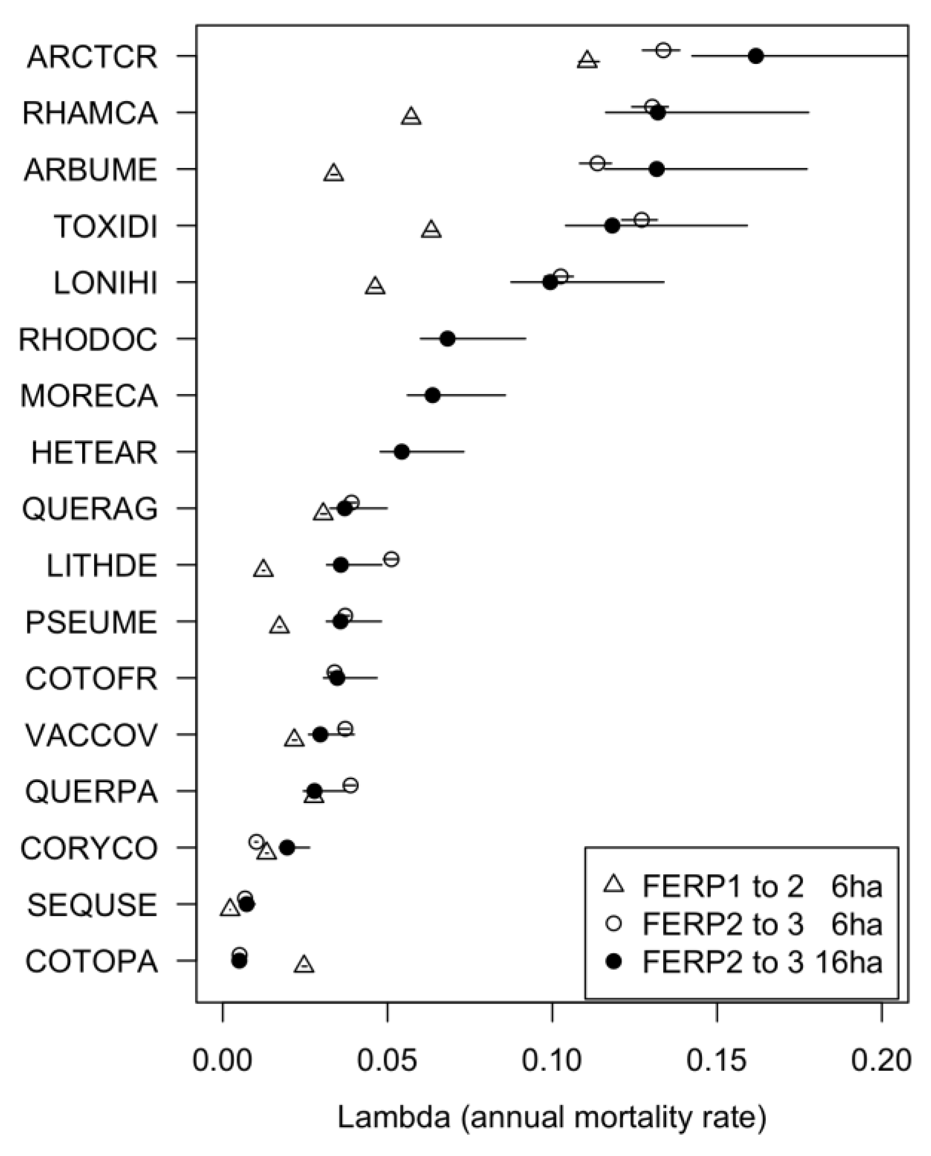
3.5. Patterns of Mortality

For all individuals of all species combined, mortality rates were greater in the second intercensus interval (FERP2 to FERP3) than in the first interval (FERP1 to FERP2). Including only individuals within the 6 ha area of the original FERP1 census, annualized mortality was 0.0270 (95% CI 0.0264–0.0279) in the first interval and 0.0532 (0.0506–0.0551). For the entire 16 ha FERP, the overall annualized mortality between FERP2 and FERP3 was 0.0398 (0.0350–0.0536).

Rates of mortality were highly variable across species and differed within species across intercensus intervals. We calculated the annualized mortality rates for all species with 20 or more live individuals in the starting census; for the 6 ha area bounded by the original FERP1 census, we calculated mortality rates for both the first and second intercensus intervals (

Table 6. Annual mortality rates for individuals on original 6 ha FERP. Lambda was calculated using the median intercensus interval; lower and upper were calculated with upper and lower 95% CI of intercensus time intervals. Lambda was not calculated for species with fewer than 20 live individuals in the starting census.

	FERP1 to FERP2					FERP2 to FERP3
			Annual Mortality					Annual Mortality
Code	Live	Surv	Lambda	Lower	Upper	Live	Surv	Lambda	Lower	Upper
ARBUME	687	585	0.0337	0.0329	0.0348	597	294	0.1137	0.1083	0.1179
ARCTCR	39	23	0.1106	0.1081	0.1142	23	10	0.1337	0.1274	0.1386
CORYCO	146	137	0.0133	0.013	0.0138	146	137	0.0102	0.0097	0.0106
COTOFR	-	-	-	-	-	21	17	0.0339	0.0323	0.0352
COTOPA	36	32	0.0247	0.0241	0.0255	32	31	0.0051	0.0049	0.0053
LITHDE	1260	1188	0.0123	0.012	0.0127	1630	1185	0.0512	0.0488	0.0531
LONIHI	217	174	0.0462	0.0452	0.0478	197	104	0.1025	0.0977	0.1063
PSEUME	2158	1988	0.0172	0.0168	0.0177	2121	1683	0.0371	0.0354	0.0385
QUERAG	908	785	0.0305	0.0298	0.0315	856	671	0.0391	0.0372	0.0405
QUERPA	1196	1048	0.0277	0.027	0.0286	1202	944	0.0388	0.0369	0.0402
RHAMCA	293	223	0.0572	0.0559	0.0590	268	119	0.1303	0.1241	0.1351
SEQUSE	190	188	0.0022	0.0022	0.0023	194	186	0.0068	0.0064	0.007
TOXIDI	675	499	0.0633	0.0618	0.0653	638	289	0.1271	0.1211	0.1318
VACCOV	254	229	0.0217	0.0212	0.0224	271	215	0.0372	0.0354	0.0385

). For the full 16 ha FERP, mortality rates could only be calculated between the FERP2 and FERP3 censuses (

Table 7. Annual mortality rates for individuals on 16 ha FERP from FERP2 to FERP3 census. Lambda was calculated using the median intercensus interval; lower and upper were calculated with upper and lower 95% CI of intercensus time intervals. Lambda was not calculated for species with fewer than 20 live individuals in FERP2.

			Annual Mortality
Code	Live	Surv	Lambda	Lower	Upper
ARBUME	845	395	0.1317	0.1159	0.1773
ARCTCR	28	11	0.1618	0.1424	0.2178
CORYCO	478	427	0.0195	0.0172	0.0263
COTOFR	22	18	0.0347	0.0306	0.0468
COTOPA	35	34	0.0050	0.0044	0.0068
HETEAR	52	38	0.0543	0.0478	0.0731
LITHDE	6164	5012	0.0358	0.0315	0.0482
LONIHI	490	276	0.0994	0.0875	0.1338
MORECA	52	36	0.0637	0.0561	0.0857
PSEUME	8005	6513	0.0357	0.0314	0.0481
QUERAG	1242	1003	0.0370	0.0326	0.0498
QUERPA	3860	3287	0.0278	0.0245	0.0375
RHAMCA	388	181	0.1320	0.1162	0.1777
RHODOC	215	145	0.0682	0.0600	0.0918
SEQUSE	2001	1919	0.0072	0.0064	0.0098
TOXIDI	1229	621	0.1182	0.104	0.1591
VACCOV	872	735	0.0296	0.0261	0.0398

). Annual mortality rates ranged from 0.2% (0.002) for Sequoia sempervirens to 16% (0.16) for Arbutus menziesii. Most species showed greater rates of mortality in the second interval than in the first (Figure 8). Differences in estimated mortality rates based on 6 ha and 16 ha areas for the second intercensus interval were similar (Table 6 and Table 7, Figure 8); they were much more similar to each other than the different rates between the two intervals for the 6 ha area.

We witnessed the extensive and dramatic standing death of Arbutus menziesii (Pacific madrone) during the second intercensus interval, reflected in a nearly 4-fold increase in annual mortality (Figure 9).

Pseudotsuga menziesii (Douglas-fir) experienced more than a doubling of the mortality rate from the first to second intercensus interval. Mortality was greater among small-diameter individuals, as would be expected from a self-thinning process (Figure 9).

The two species of Quercus (oaks), as well as Sequoia sempervirens (redwood), did not show significant increases in mortality during the second intercensus interval. Mortality for oaks was relatively flat across diameter categories (Figure 9). Redwood had very low levels of mortality, but they were greater among small-diameter individuals (Figure 9).

3.6. Patterns of Recruitment

New individuals are recruited into the FERP data set when they reach 1 cm in diameter at standard height. In the first intercensus interval (FERP1 to FERP2), new recruits slightly exceeded the number of deaths, for a net 1.08% increase in living individuals (

Table 8. Number of individuals of each species that died or were recruited (dsh ≥ 1 cm) in each intercensus interval. Data limited to the 6 ha region of the FERP1 census are shown for both intervals, and for the second interval, data for the entire 16 ha FERP are also shown. Data are presented for each species, the number of live individuals at the start of the interval, the number of those individuals that died, the number of newly recruited individuals, and the change in live individuals (recruits–deaths).

	FERP1 to FERP2 6 ha				FERP2 to FERP3 6 ha				FERP2 to FERP3 16 ha
Code	Live	Died	Recruit	R-D	Live	Died	Recruit	R-D	Live	Died	Recruit	R-D
ACERMA	2	0	0	0	2	0	0	0	10	1	0	−1
ADENFA	- 1	-	-	-	-	-	-	-	1	1	0	−1
ARBUME	687	102	12	−90	597	303	7	−296	845	450	16	−434
ARCTAN	11	4	0	−4	7	7	1	−6	9	8	10	2
ARCTCR	39	16	0	−16	23	13	0	−13	28	17	1	−16
BACCPI	11	10	0	−10	1	1	1	0	6	5	13	8
CEANTH	1	0	0	0	1	1	0	−1	2	1	1	0
CORYCO	146	9	9	0	146	9	17	8	478	51	49	−2
COTOFR	18	0	3	3	21	4	0	−4	22	4	1	−3
COTOPA	36	4	0	−4	32	1	2	1	35	1	4	3
CRATMO	1	0	0	0	1	0	0	0	1	0	0	0
ERIOJA	-	-	-	-	-	-	-	-	1	0	0	0
EUCAGL	5	0	0	0	5	0	0	0	6	0	0	0
HEDEHE	8	2	1	−1	7	0	5	5	11	1	6	5
HETEAR	11	5	2	−3	8	0	3	3	52	14	12	−2
ILEXAQ	10	1	0	−1	9	1	2	1	13	2	4	2
LITHDE	1260	72	442	370	1630	445	305	−140	6164	1152	1288	136
LONIHI	217	43	23	−20	197	93	19	−74	490	214	39	−175
MORECA	8	1	1	0	8	5	0	−5	52	16	3	−13
PINUAT	1	1	0	−1	0	0	0	0	3	0	0	0
PINUPO	17	7	0	−7	10	3	0	−3	15	3	1	−2
PSEUME	2158	170	133	−37	2121	438	164	−274	8005	1492	778	−714
PYRAAN	1	0	0	0	1	0	0	0	1	0	0	0
QUERAG	908	123	71	−52	856	185	68	−117	1242	239	146	−93
QUERPA	1196	148	151	3	1202	258	236	−22	3860	573	1448	875
RHAMCA	293	70	45	−25	268	149	27	−122	388	207	53	−154
RHODOC	-	-	-	-	-	-	-	-	215	70	5	−65
RIBEDI	1	0	0	0	1	1	0	−1	3	1	1	0
SALILA	2	0	0	0	2	0	0	0	4	1	1	0
SAMBNI	2	0	0	0	2	1	0	−1	3	1	1	0
SEQUSE	190	2	6	4	194	8	9	1	2001	82	95	13
TOXIDI	675	176	139	−37	638	349	42	−307	1229	608	101	−507
UMBECA	11	0	0	0	11	1	0	−1	16	2	0	−2
VACCOV	254	25	42	17	271	56	17	−39	872	137	49	−88
Total	8180	991	1080	89	8272	2332	925	−1407	26,083	5354	4126	−1228

¹ Species not found in the 6 ha region.

). In the same 6 ha region, the number of recruits (in total and across species) was similar in the second interval (FERP2 to FERP3), but recruitment was far eclipsed by the number of deaths, leading to a 17.0% decrease in the number of living stems, driven primarily by strong recruit–death differentials in Arbutus menziesii, Notholithocarpus densiflorus, Pseudotsuga menziesii, Frangula californica, and Toxicodendron diversilobum (Table 8). This pattern was consistent but more muted across the entire 16 ha in the second interval, with an overall 4.71% decline in live stems. In the eastern part of the FERP, N. densiflorus is abundant and had low mortality, so recruitment outpaced death on the 16 ha FERP.

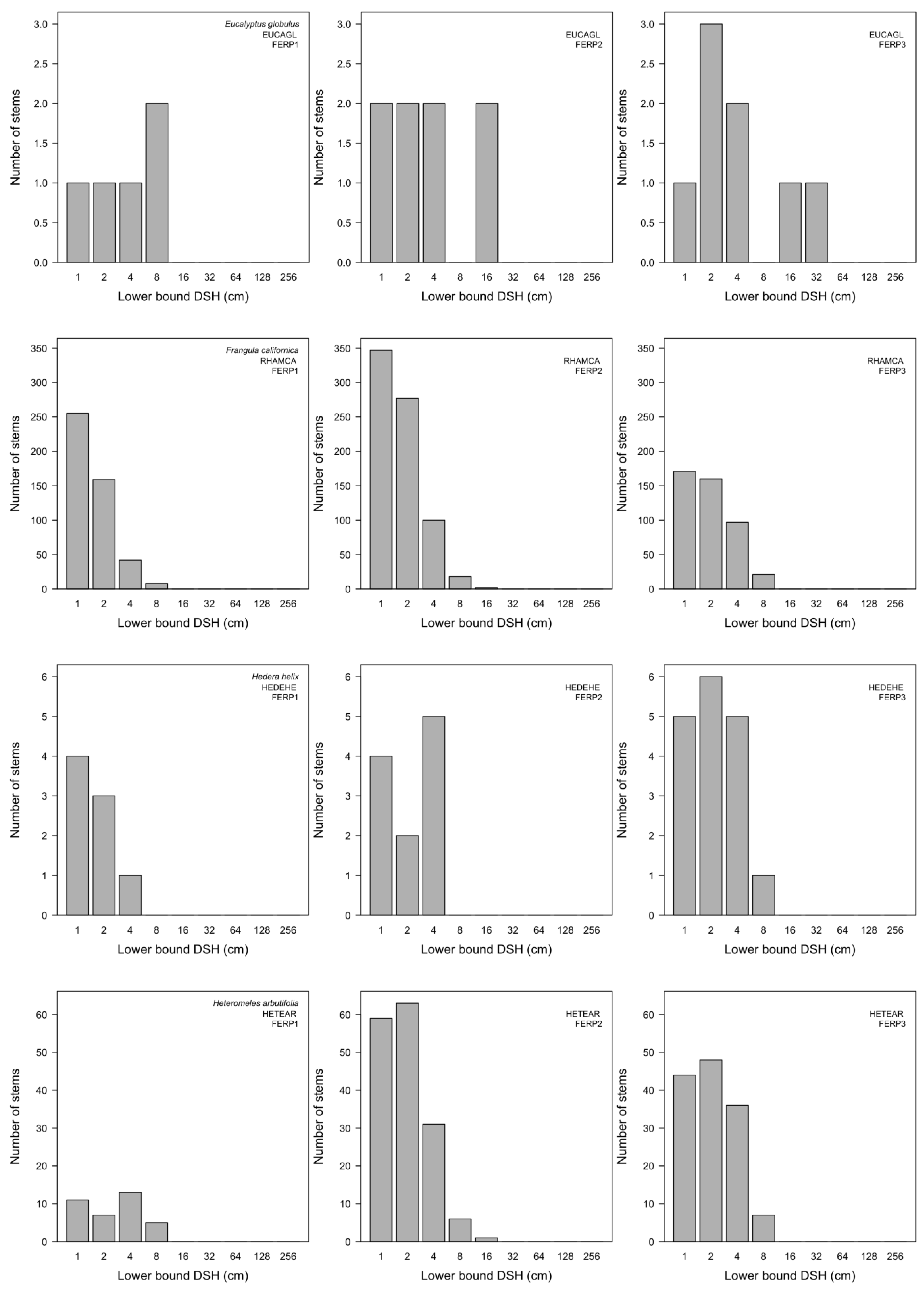
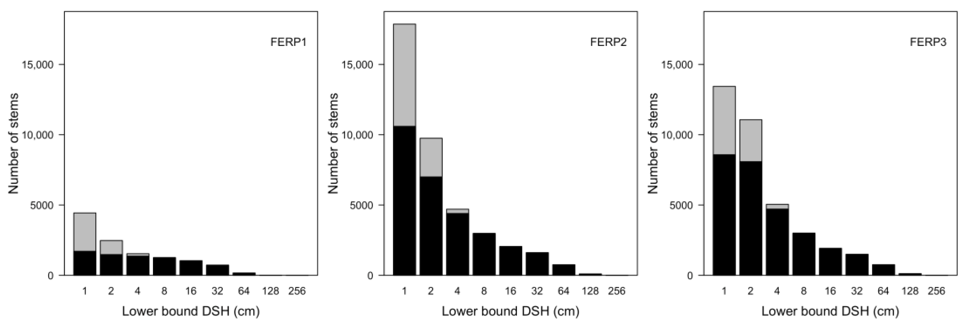
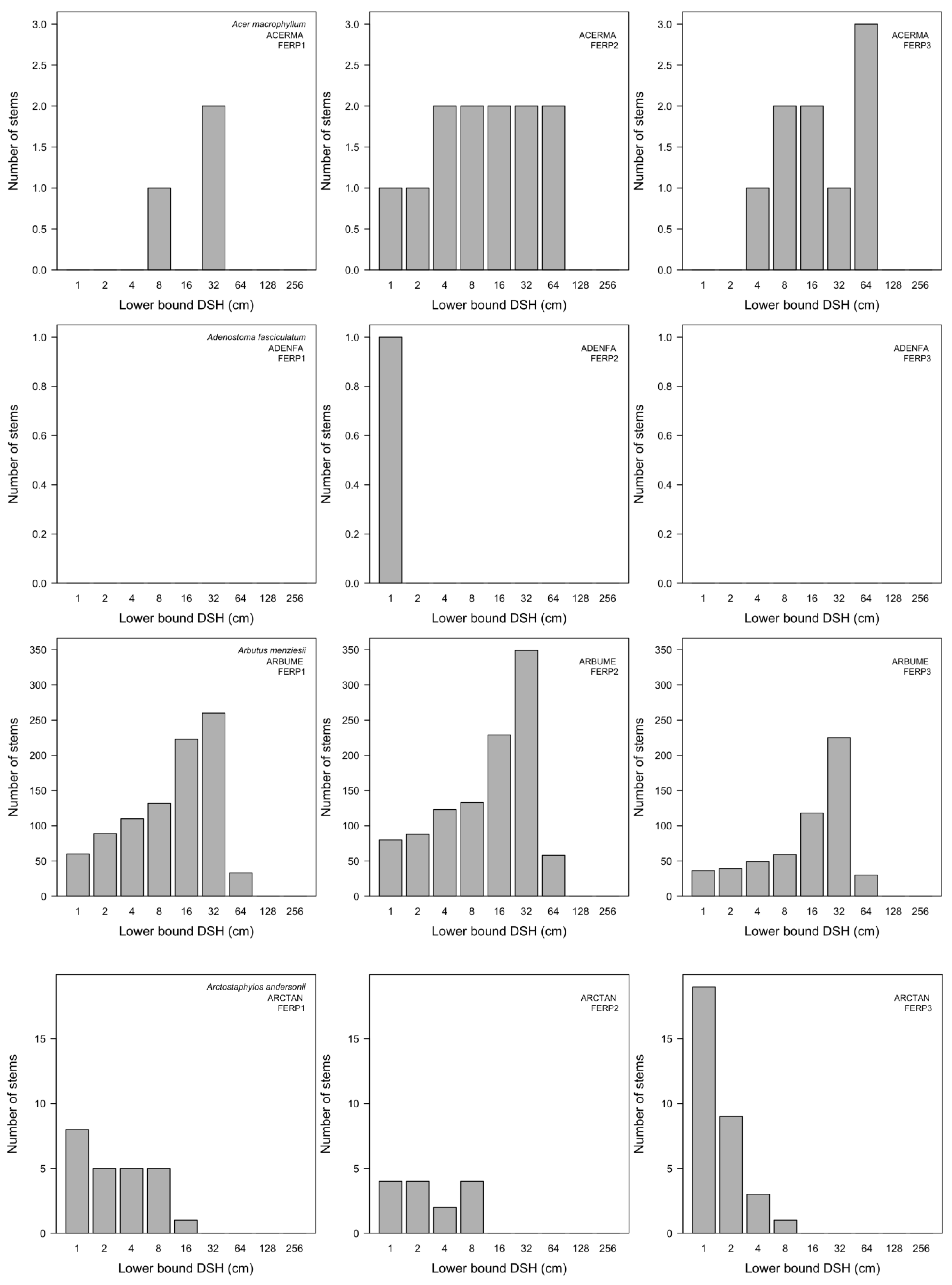
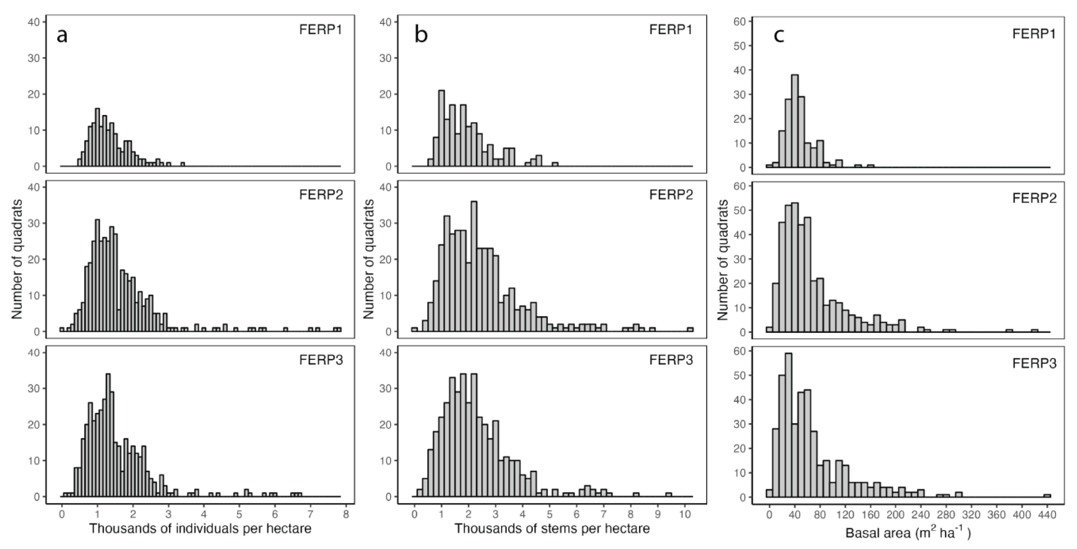
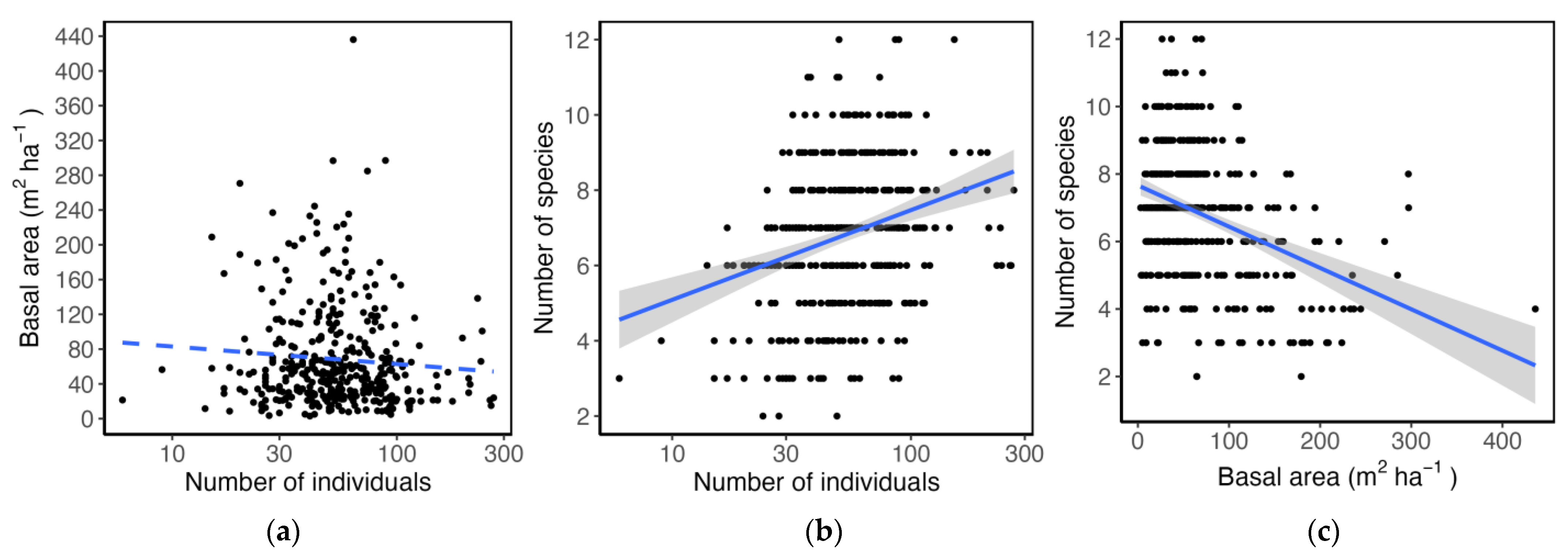
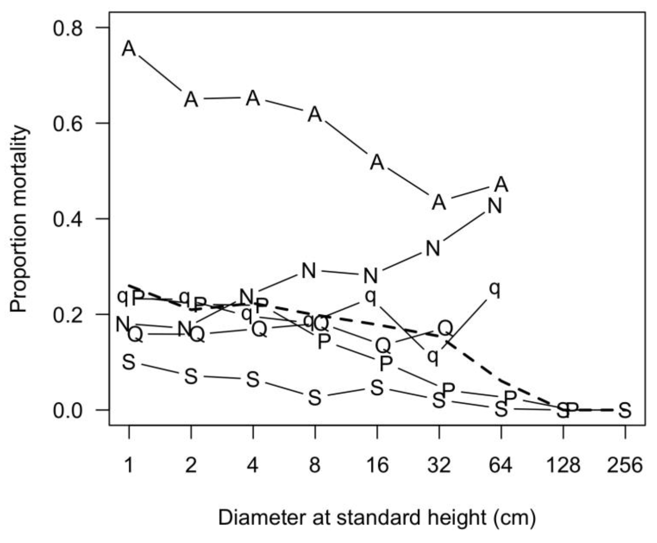
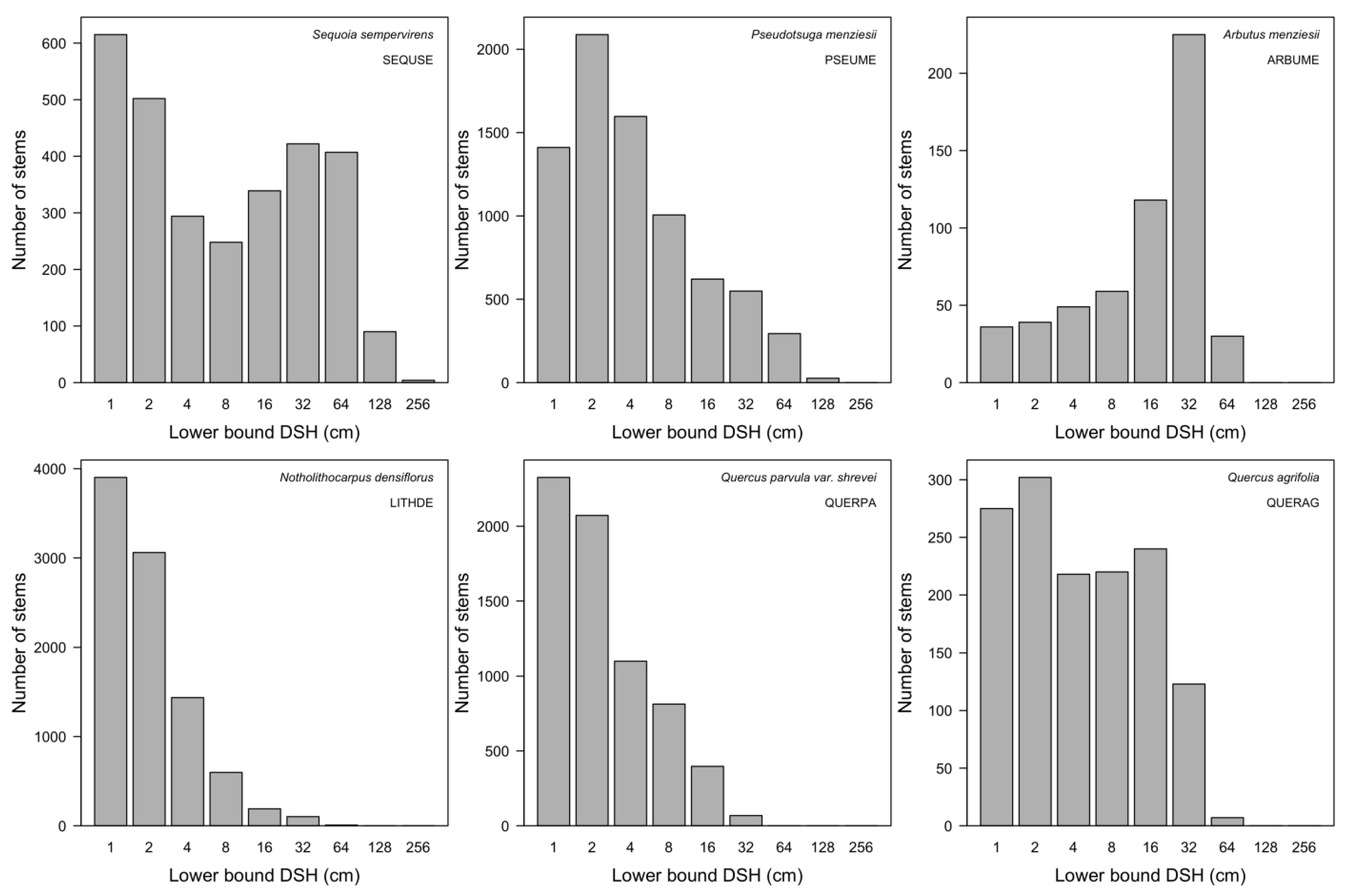
3.7. Patterns of Size Distribution

The overall stem-diameter distribution of woody plants of all species on the FERP follows the typical right-skewed (positive-skewed) distribution pattern of forest communities (Figure 10). Shrubs and lianas form a significant proportion of the smallest size classes, together representing 33.7%, 26.1%, and 22.4% of all stems in FERP1, FERP2, and FERP3 censuses, respectively. The combination of the disproportionate mortality of smaller stems (Figure 9), limited recruitment (Table 8), and the transition of some surviving stems into larger size classes created a shift to a somewhat more even class-size distribution from FERP2 to FERP3 (Figure 10).

The six most abundant species on the FERP (Figure 5b and Figure 6) include the range of possible stem-diameter distribution patterns (Figure 11), from strongly right-skewed (Pseudotsuga, Notholithocarpus, and Quercus parvula) to left-skewed (Arbutus), as well as bimodal (Sequoia) and flat (Quercus agrifolia). The stem-size distribution figures for each species in each of the three censuses are provided in Appendix H (Figure A7).

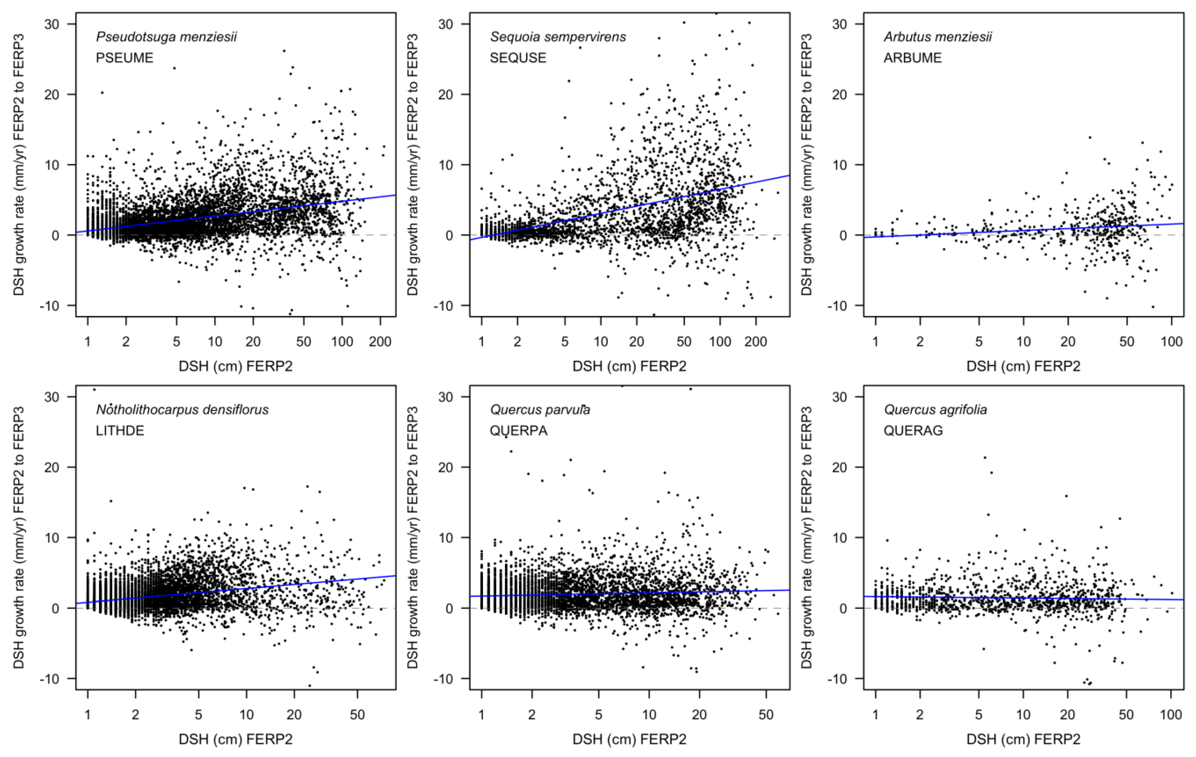
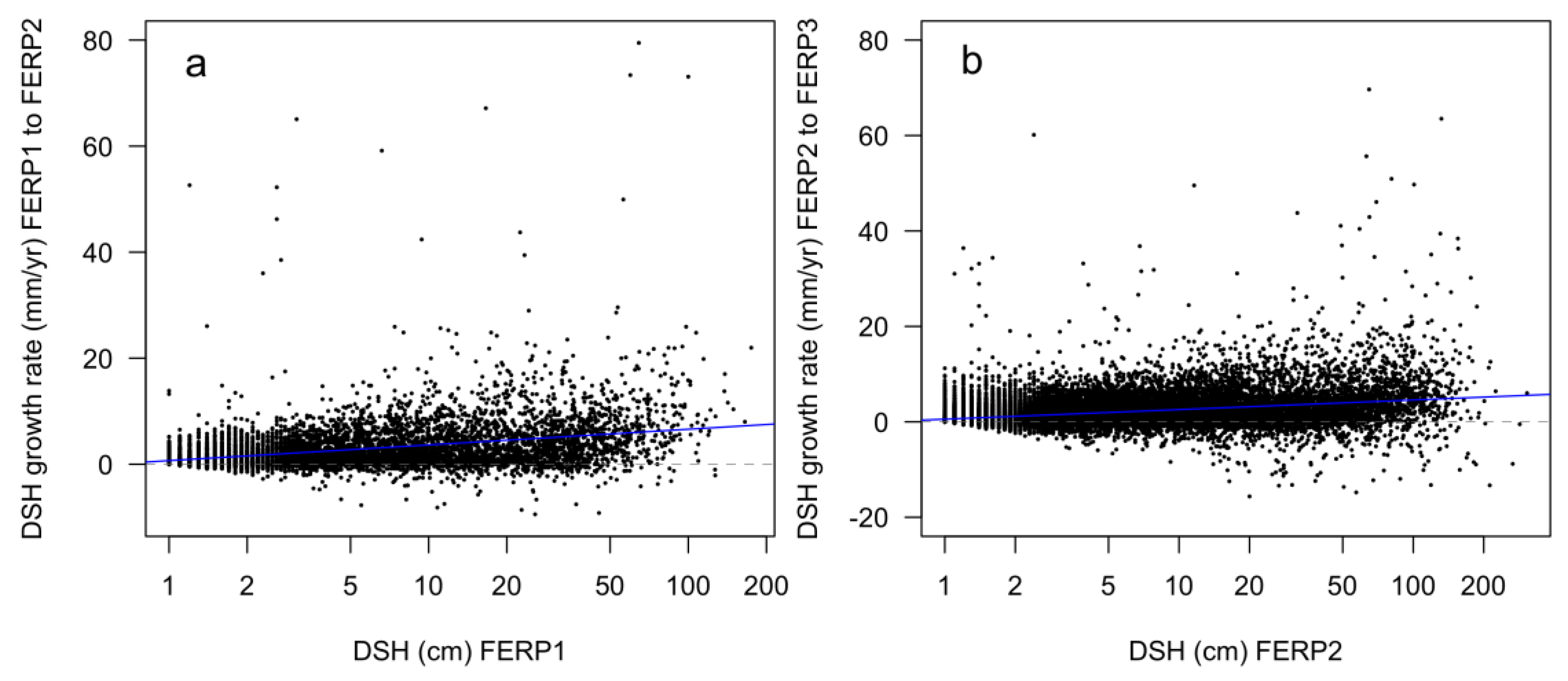
3.8. Patterns of Growth

The absolute annual diameter growth rate increased with increasing initial stem diameter (Figure 12). Each of the six most abundant species showed a significant positive growth rate, and for all species except Quercus agrifolia, larger individuals grew significantly more rapidly (Figure 13). Regression coefficients and statistics for all species (n ≥ 10 stems) in the 6 ha area for FERP1 to FERP2 and for FERP2 to FERP3, as well as in the full 16 ha for FERP2 to FERP3, are presented in Appendix I (

Table A1. Linear regression coefficients and statistics for annual growth (diameter in mm yr⁻¹) as a function of log₁₀(diameter) (in cm). Only species with 10 or more individuals at the start of the interval are included. Data limited to the 6 ha region of the FERP1 census are shown for both intervals, and for the second interval, data for the entire 16 ha FERP are also shown.

Interval and Area	Code6	Intercept	Slope	F	dfresid	R2adj	p
FERP1 to 2 6 ha	ARBUME	0.0510	0.8264	2.266	284	0.004	0.13339
FERP1 to 2 6 ha	CORYCO	0.5430	−0.4565	1.818	108	0.007	0.18042
FERP1 to 2 6 ha	COTOFR	−0.1549	1.3384	1.628	11	0.050	0.22828
FERP1 to 2 6 ha	COTOPA	0.6771	0.8726	0.365	23	−0.027	0.55159
FERP1 to 2 6 ha	LITHDE	0.7194	3.4134	145.686	834	0.148	<0.00001
FERP1 to 2 6 ha	LONIHI	0.5059	0.0256	0.002	91	−0.011	0.96401
FERP1 to 2 6 ha	PSEUME	0.0367	2.6748	241.779	1571	0.133	<0.00001
FERP1 to 2 6 ha	QUERAG	1.6715	−0.4876	4.648	597	0.006	0.03148
FERP1 to 2 6 ha	QUERPA	1.7115	0.3153	1.820	796	0.001	0.17771
FERP1 to 2 6 ha	RHAMCA	0.6775	2.7735	10.480	78	0.107	0.00177
FERP1 to 2 6 ha	SEQUSE	−2.5797	8.1291	164.955	176	0.481	<0.00001
FERP1 to 2 6 ha	TOXIDI	0.4083	0.0621	0.013	210	−0.005	0.91000
FERP1 to 2 6 ha	VACCOV	0.7504	0.0311	0.003	166	−0.006	0.95896
FERP2 to 3 6 ha	ARBUME	0.0668	0.7163	2.944	356	0.005	0.08707
FERP2 to 3 6 ha	ARCTCR	2.9091	−3.8892	2.516	11	0.112	0.14102
FERP2 to 3 6 ha	CORYCO	0.6603	−0.8901	31.354	685	0.042	<0.00001
FERP2 to 3 6 ha	COTOFR	1.0233	−1.1838	3.119	30	0.064	0.08754
FERP2 to 3 6 ha	COTOPA	1.7131	−0.2399	0.088	48	−0.019	0.76757
FERP2 to 3 6 ha	HETEAR	2.6800	−2.0952	0.791	13	−0.015	0.39005
FERP2 to 3 6 ha	ILEXAQ	0.3698	2.4993	6.654	10	0.340	0.02744
FERP2 to 3 6 ha	LITHDE	0.8468	3.1792	352.477	1528	0.187	<0.00001
FERP2 to 3 6 ha	LONIHI	0.6395	−0.2672	0.249	112	−0.007	0.61906
FERP2 to 3 6 ha	PSEUME	0.5714	2.2955	225.324	1709	0.116	<0.00001
FERP2 to 3 6 ha	QUERAG	1.6917	−0.5010	8.601	738	0.010	0.00346
FERP2 to 3 6 ha	QUERPA	1.7007	0.2501	2.355	1264	0.001	0.12510
FERP2 to 3 6 ha	RHAMCA	1.6583	1.4043	5.420	171	0.025	0.02108
FERP2 to 3 6 ha	SEQUSE	−1.6736	7.1713	231.511	234	0.495	<0.00001
FERP2 to 3 6 ha	TOXIDI	0.5572	−0.2852	0.293	307	−0.002	0.58889
FERP2 to 3 6 ha	VACCOV	0.7292	−0.7583	12.114	775	0.014	0.00053
FERP2 to 3 16 ha	ARBUME	−0.2682	0.9131	7.357	486	0.013	0.00692
FERP2 to 3 16 ha	ARCTCR	3.0971	−4.0288	2.944	12	0.130	0.11186
FERP2 to 3 16 ha	CORYCO	0.6802	−1.0401	45.541	2450	0.018	<0.00001
FERP2 to 3 16 ha	COTOFR	1.2554	−1.6360	3.984	31	0.085	0.05478
FERP2 to 3 16 ha	COTOPA	1.5556	−0.0346	0.002	51	−0.020	0.96319
FERP2 to 3 16 ha	HETEAR	1.3254	−0.3766	0.204	92	−0.009	0.65222
FERP2 to 3 16 ha	ILEXAQ	0.3865	2.2146	4.476	14	0.188	0.05278
FERP2 to 3 16 ha	LITHDE	0.8149	1.9323	721.803	7337	0.089	<0.00001
FERP2 to 3 16 ha	LONIHI	0.5321	−0.5910	3.507	297	0.008	0.06208
FERP2 to 3 16 ha	MORECA	0.2690	1.7740	8.310	62	0.104	0.00541
FERP2 to 3 16 ha	PINUPO	−5.6189	8.2716	43.530	10	0.795	0.00006
FERP2 to 3 16 ha	PSEUME	0.5880	2.1073	1016.673	6670	0.132	<0.00001
FERP2 to 3 16 ha	QUERAG	1.6028	−0.2101	1.495	1139	0.000	0.22174
FERP2 to 3 16 ha	QUERPA	1.6734	0.4623	27.311	4604	0.006	0.00001
FERP2 to 3 16 ha	RHAMCA	1.5007	1.1883	6.606	325	0.017	0.01061
FERP2 to 3 16 ha	RHODOC	0.2906	−0.6306	6.276	435	0.012	0.01260
FERP2 to 3 16 ha	SEQUSE	−0.3350	3.4143	578.488	2737	0.174	<0.00001
FERP2 to 3 16 ha	TOXIDI	0.5124	−0.7535	6.951	663	0.009	0.00857
FERP2 to 3 16 ha	UMBECA	2.7814	−3.7592	2.553	13	0.100	0.13410
FERP2 to 3 16 ha	VACCOV	0.5880	−0.8690	57.947	2417	0.023	<0.00001

). Of the 49 species/intervals that could be tested, 17 showed statistically significant positive slopes, and 8 showed negative slopes, with the majority showing no effect of diameter on the growth rate. In contrast, 33 showed significantly negative slopes for size-dependent relative growth rates, and just 4 showed positive slopes, including negative slopes for each of the 6 most abundant species in all but two comparisons (

Table A2. Linear regression statistics for annual relative growth rate (cm cm⁻¹ yr⁻¹) as a function of log₁₀(diameter) (in cm). Only species with ≥10 individuals at the start of the interval are included. Results presented for the 6 ha region of the FERP1 census for both intervals and the entire 16 ha FERP for the second interval.

Interval and Area	Code6	Intercept	Slope	F	dfresid	R2adj	p
FERP1 to 2 6 ha	ARBUME	0.0304	−0.0104	10.5504	574	0.016	0.00123
FERP1 to 2 6 ha	ARCTCR	−0.0140	0.0229	0.6400	20	−0.017	0.43310
FERP1 to 2 6 ha	CORYCO	0.0031	0.0157	0.9613	128	0.000	0.32870
FERP1 to 2 6 ha	COTOFR	−0.0035	0.0506	1.4018	15	0.024	0.25485
FERP1 to 2 6 ha	COTOPA	0.0334	−0.0071	0.1076	26	−0.034	0.74552
FERP1 to 2 6 ha	LITHDE	0.0876	0.0030	0.2948	1179	−0.001	0.58725
FERP1 to 2 6 ha	LONIHI	−0.0090	0.1456	43.2717	172	0.196	<0.00001
FERP1 to 2 6 ha	PSEUME	0.0605	−0.0214	118.0180	1979	0.056	<0.00001
FERP1 to 2 6 ha	QUERAG	0.0458	−0.0249	66.5674	777	0.078	<0.00001
FERP1 to 2 6 ha	QUERPA	0.0600	−0.0310	53.4449	1031	0.048	<0.00001
FERP1 to 2 6 ha	RHAMCA	0.0154	0.1214	43.3036	215	0.164	<0.00001
FERP1 to 2 6 ha	SEQUSE	0.0440	0.0028	0.2814	184	−0.004	0.59642
FERP1 to 2 6 ha	TOXIDI	−0.0015	0.1356	109.9723	494	0.180	<0.00001
FERP1 to 2 6 ha	UMBECA	0.0012	0.0269	1.3054	8	0.033	0.28627
FERP1 to 2 6 ha	VACCOV	−0.0050	0.0622	11.5952	222	0.045	0.00078
FERP2 to 3 6 ha	ARBUME	0.0207	−0.0117	31.3512	356	0.078	<0.00001
FERP2 to 3 6 ha	ARCTCR	0.0578	−0.0629	9.6636	11	0.419	0.00995
FERP2 to 3 6 ha	CORYCO	0.0428	−0.0813	106.1102	685	0.133	<0.00001
FERP2 to 3 6 ha	COTOFR	0.0667	−0.1142	13.9856	30	0.295	0.00078
FERP2 to 3 6 ha	COTOPA	0.0908	−0.0890	22.9697	48	0.310	0.00002
FERP2 to 3 6 ha	HETEAR	0.0656	−0.0617	1.3157	13	0.022	0.27204
FERP2 to 3 6 ha	ILEXAQ	0.0489	−0.0230	0.5328	10	−0.044	0.48217
FERP2 to 3 6 ha	LITHDE	0.0631	−0.0242	46.5612	1528	0.029	<0.00001
FERP2 to 3 6 ha	LONIHI	0.0461	−0.0759	10.4039	112	0.077	0.00165
FERP2 to 3 6 ha	PSEUME	0.0593	−0.0319	516.2390	1709	0.232	<0.00001
FERP2 to 3 6 ha	QUERAG	0.0640	−0.0445	366.4589	738	0.331	<0.00001
FERP2 to 3 6 ha	QUERPA	0.0775	−0.0565	435.9180	1264	0.256	<0.00001
FERP2 to 3 6 ha	RHAMCA	0.0942	−0.0750	17.9495	171	0.090	0.00004
FERP2 to 3 6 ha	SEQUSE	0.0283	−0.0016	0.2948	234	−0.003	0.58768
FERP2 to 3 6 ha	TOXIDI	0.0414	−0.0895	20.1884	307	0.059	0.00001
FERP2 to 3 6 ha	UMBECA	0.0371	0.0010	0.0005	9	−0.111	0.98227
FERP2 to 3 6 ha	VACCOV	0.0507	−0.0998	114.2036	775	0.127	<0.00001
FERP2 to 3 16 ha	ARBUME	0.0150	−0.0082	20.9983	486	0.039	0.00001
FERP2 to 3 16 ha	ARCTCR	0.0614	−0.0656	10.6471	12	0.426	0.00679
FERP2 to 3 16 ha	CORYCO	0.0409	−0.0808	260.2206	2450	0.096	<0.00001
FERP2 to 3 16 ha	COTOFR	0.0758	−0.1320	13.7912	31	0.286	0.00080
FERP2 to 3 16 ha	COTOPA	0.0848	−0.0811	21.6265	51	0.284	0.00002
FERP2 to 3 16 ha	HEDEHE	0.0842	−0.0627	2.6679	8	0.156	0.14103
FERP2 to 3 16 ha	HETEAR	0.0594	−0.0587	6.9670	92	0.060	0.00975
FERP2 to 3 16 ha	ILEXAQ	0.0524	−0.0325	1.1025	14	0.007	0.31150
FERP2 to 3 16 ha	LITHDE	0.0562	−0.0288	266.7038	7337	0.035	<0.00001
FERP2 to 3 16 ha	LONIHI	0.0387	−0.0808	26.9351	297	0.080	<0.00001
FERP2 to 3 16 ha	MORECA	0.0304	−0.0069	0.0687	62	−0.015	0.79404
FERP2 to 3 16 ha	PINUPO	0.0222	−0.0043	0.2605	10	−0.072	0.62086
FERP2 to 3 16 ha	PSEUME	0.0556	−0.0308	957.6681	6670	0.125	<0.00001
FERP2 to 3 16 ha	QUERAG	0.0643	−0.0445	328.8228	1139	0.223	<0.00001
FERP2 to 3 16 ha	QUERPA	0.0881	−0.0674	1114.4110	4604	0.195	<0.00001
FERP2 to 3 16 ha	RHAMCA	0.0878	−0.0725	26.4437	325	0.072	<0.00001
FERP2 to 3 16 ha	RHODOC	0.0196	−0.0568	24.3796	435	0.051	<0.00001
FERP2 to 3 16 ha	SEQUSE	0.0266	−0.0090	98.8974	2737	0.035	<0.00001
FERP2 to 3 16 ha	TOXIDI	0.0384	−0.1002	60.2448	663	0.082	<0.00001
FERP2 to 3 16 ha	UMBECA	0.0775	−0.0727	5.8115	13	0.256	0.03145
FERP2 to 3 16 ha	VACCOV	0.0418	−0.0940	276.5557	2417	0.102	<0.00001

). Overall, larger individuals had greater absolute radial growth, but relative to their size, larger individuals usually grew less than smaller ones.

4. Discussion

4.1. Species Composition

The UC Santa Cruz FERP includes areas representative of the two most common forest types on and near the UC Santa Cruz campus [35]. The western half of the FERP is most closely aligned with the “Douglas fir—tanoak forest—madrone forest and woodland alliance”, while the eastern part allies with the “Redwood forest and woodland alliance” of the California Native Plant Society [40]. While the FERP vegetation represents most of the woody species on the campus, there are a few notable exceptions. Although the southeast corner of the FERP includes a small perennial stream, it lacks a well-developed riparian forest and associated riparian species such as Populus trichocarpa, Aesculus californica, and several species of Salix. Those riparian species are present in a much wetter, nearly swamp forest found at the southernmost extent of the campus, about 3 km distant. The FERP is also missing a few less common tree species found elsewhere on the Campus Natural Reserve, including Quercus × morehus, Acer negundo, Chrysolepsis chrysophylla, and the invasive species Acacia dealbata, A. melanoxylon, and Genista monspessulana. Each of these species is patchy and locally uncommon in the landscape; unlike for the riparian species, there are no obvious environmental limitations, and they are most likely missing from the FERP by chance distribution. The FERP is also missing a number of woody shrubs that are limited to high-light chaparral habitat elsewhere on the campus; they are unlikely to be able to thrive in the dark habitat of the forest.

All of the invasive species are frequently found in the Santa Cruz area as horticultural plantings and as forest invaders. Both Eucalyptus globulus and Ilex aquifolium are abundant in the planted landscape of the nearby Cave Gulch community. Both species of Cotoneaster are found as planted hedges throughout the Santa Cruz area and are commonly found as forest understory volunteers. The single individual of loquat (Eriobotrya japonica) may be a natural dispersal from garden trees planted throughout Santa Cruz or the product of a discarded seed from someone’s lunch. The overall abundance of non-native woody species in the FERP is quite low (<0.5% of the stems and 0.04% of the basal area) compared to nearby grasslands, which are dominated by non-native European species [35]. We are conscious of the potential ecological impacts of expanding populations of non-native woody species (e.g., [41,42,43,44]). Nevertheless, we have taken the approach of not attempting to control populations of non-native species on the FERP based on the judgment that the potential value of what we can learn about their spread and their impacts on the forest outweighs environmental threats from species that are already common in the surrounding landscape.

4.2. Abundance and Basal Area

The FERP forest appears to be in a self-thinning phase following disturbances over the last 140 years or so; the total number of individuals and stems is decreasing, while the overall basal area is increasing. Disturbances vary in type and timing, including clear-cut logging of the redwood forest in the late 1800s and early 1900s [31,35], a low-intensity, 4 ha fire in the eastern part of the FERP in 1964 [34], and multi-species, canopy-level dieback of unknown cause in the northern part of the FERP in the first decade of the current century (Figure A4). Such disturbances allow the establishment of seedlings and saplings at greater densities than can establish in the closed-canopy forest. Some 20 m × 20 m quadrats in the dieback areas have extraordinary stem densities of small-diameter Pseudotsuga menziesii that approach 1 stem per m²; we expect such areas, apparent in the long right-hand tails of Figure 3a,b, to undergo rapid self-thinning through density-dependent processes in the coming years. For light-demanding species such as Arbutus menziesii and resprouting species like Sequoia sempervirens, large disturbances can create the opportunity for pulsed recruitment.

There was no significant relationship between the number of individuals and total basal area within quadrats across all species. Instead, a high basal area density was associated with areas with few large-diameter trees (often Sequoia sempervirens or Pseudotsuga menziesii), rather than a large number of stems. This is consistent with global patterns, where large-diameter trees make up about half the woody biomass but less than 1% of the individuals in mature forests worldwide [45].

Species richness increased with the increasing number of individuals in a quadrat. This is a common pattern in forest communities, where local diversity increases with individual density because sampling a greater number of individuals increases the chances of encountering additional species that are present in the community [46]. However, species richness also decreased with increasing basal area. Areas of the forest with the greatest basal area were dominated by large Sequoia or Pseudotsuga trees, which were also tall trees that created a deeply shaded understory, limiting the opportunity for the recruitment of many shade-intolerant species [47]. On the FERP, an additive model that included both the abundance and basal area better described the patterns of species richness.

4.3. Structure and Species Relative Abundance

Large-diameter and abundant tree species have dominant impacts on forest structure [48], and the largest species on the FERP are also the most abundant. The six most numerically abundant tree species (Figure 5, Table 3; 77.4% of all stems and 99.7% of all tree stems alive in FERP3) also include 99.1% of all stems larger than 64 cm diameter (n = 874) and represent 99.5% of all stems larger than 32 cm (n = 2368). Just Sequoia and Pseudotsuga alone represent 93.9% of those largest stems. The remaining large-diameter species on the FERP (Acer macrophyllum, Eucalyptus globulus, Pinus attenuata, and P. ponderosa) are all rare, collectively representing only 0.06% of the stems on the FERP.

The understory shrub community represents 19.2% of all the stems and over half the woody species on the FERP. Several of the shrub species are light-demanding species most commonly found in nearby grassland or chaparral habitats (Adenostoma fasciculatum, Arctostaphylos andersonii, Arctostaphylos crustacea subsp. crinita, Baccharis pilularis, Ceanothus thyrsiflorus); these species are rare in the FERP, mostly associated with higher-light, disturbed areas. Four of the eighteen species of shrubs are introduced, invasive species from the Rosaceae family (Cotoneaster franchetii, C. pannosus, Crataegus monogyna, Pyracantha angustifolia); there are no native shrubs from this family on the FERP.

The most abundant liana on the FERP is poison oak (Toxicodendron diversilobum). In high-light conditions, T. diversilobum can grow as a shrub, but its dominant growth form in the forest is as a liana. Poison oak makes up more than two-thirds of the liana stems and 2.1% of all stems in FERP3. This is, however, a great underestimate of the abundance of this species in the plot, because the vast majority of stems of this nearly omnipresent species do not reach the standard height for measurement. There is no such obvious abundance underestimation for any other measured species on the FERP.

4.4. Spatial Patterns

The dominant spatial pattern is the transition from the western mixed-evergreen forest (a mixed canopy of Quercus spp., Pseudotsuga, and Arbutus) to the eastern forest with a canopy of Sequoia, some Pseudotsuga, and a subcanopy of Notholithocarpus (Figure 6). The redwood-rich eastern forest was clear-cut more than a century ago and experienced an understory wildfire in 1964; the combination of redwood resprouting and subsequent seedling recruitment has maintained redwood dominance, with large trees that create a deeply shaded understory. In contrast, the western forest experienced neither of these stand-level disturbances; we suspect this part of the forest may represent succession from meadow and chaparral habitats still found nearby. The different shapes of Quercus and Pseudotsuga trees (short and broad vs. tall and narrow) in this western region create a visibly more uneven canopy structure and understory light environment. Associated with this pattern is a decline in species richness from west to east (Figure 7).

Notably, the three species of Fagaceae have complementary spatial patterns in the forest (Figure 6 and Figure A5). Quercus parvula var. shrevei and Q. agrifolia have known differences in environmental preferences, with Q. parvula preferring wetter environments [49] and Notholithocarpus preferring moister conditions than Quercus spp. [50]. These three close relatives provide an opportunity for future work on how environmental filters shape spatial patterns in the coastal California forest. In addition, the two species of Quercus are known to hybridize [49]. We identify the two species morphologically based on the preponderance of diagnostic leaf traits in an individual; there would be value in future work to evaluate genetic introgression and differential responses to environmental gradients at the genotype level.

There are three areas of apparent successional change on the FERP. The first is the apparent decline of a remnant chaparral community in the south-central FERP. Arctostaphylos crustacea has the highest rate of mortality of any species on the FERP (Figure 8), and the rare individuals of other chaparral species in this patch (A. andersonii, Pinus attenuata, and Ceanothus thyrsiflorus) mostly died as well (Table 8, Figure A5). These same species are thriving outside the FERP, a few hundred meters south in open, high-light chaparral habitat, but are apparently unable to survive in the shaded understory of tall, mature Douglas-fir.

The other two areas of successional change are in the northern part of the FERP. These ~0.6 ha areas are associated first with a rapid, multi-species canopy decline event in 2004–2006, which then extended westward from 2008 to 2010 (Figure A4). The cause of this mortality is not known, as we were not working in that area of the forest during those years. At the time of FERP2 establishment, the eastern area was filled with a very high density of Pseudotsuga saplings—an average distance of 0.64 m between Douglas-fir individuals in quadrat E280_N320 (Figure 2b and Figure 6). In contrast, the western area had little canopy cover and the remains of many large, dead standing and fallen trees. There were few living woody plants, with an average distance of 2.774 m between individuals of any species in quadrat E160_N380, and only one individual larger than 15 cm. The coming years should show strong dynamics in these patches, with self-thinning among the dense Douglas-fir and the rapid recruitment of individuals into the western patch.

4.5. Patterns of Mortality

Mortality rates varied greatly among species (Figure 8) and were greater for nearly all species in the second intercensus interval (~2012–2018) than in the first (~2007–2012) (6 ha region only, Table 6). Santa Cruz experienced two drought periods during that time, first in 2007–2009 and then in 2012–2015, along with two periods of much greater than average rainfall (2010 and 2016–2017). The 5 yr temporal resolution of FERP censuses does not permit the attribution of mortality patterns to such variation in precipitation, but high levels of precipitation are associated with a greater spread of pathogens [51], and drought is commonly associated with tree mortality [52,53,54], particularly of trees suffering from root and vascular pathogens [55].

Three tree species showed large increases in mortality rates during the second intercensus interval; all were strikingly apparent in the forest because of the unusual number of standing dead trees. Notholithocarpus densiflorus (tanoak) showed a pattern of death consistent with sudden oak death (SOD), caused by the invasive oomycete pathogen Phytophthora ramorum [56]. Infected trees progressed from apparently healthy to dead in a few months but retained a full crown of dead, brown leaves for a year or more. Diagnostic cankers of SOD were common on the dead trees. The first symptoms of SOD appeared shortly after the FERP1 census and increased dramatically in the following years. Tanoak mortality increased 5-fold between the first and second intervals. The disease progressed more rapidly among larger individuals (Figure 9), a known pattern for SOD [57].

Arbutus menziesii suffered a 4-fold increase in mortality rate from the first to the second intercensus interval, with large trees showing signs of branch dieback and then dying while standing. The cause of the mortality is not yet known, but large trees suffer high rates of apparent root and butt rot, together with necrotic foliar diseases on individuals of all sizes; regionally, madrones have been in decline for several decades [58].

4.6. Patterns of Recruitment

Half of the 34 species on the FERP showed more mortality than recruitment, and an additional 9 showed no net change in numbers (Table 8); across the FERP, there was a 4.7% decrease in the number of living stems. The largest net increases were for Quercus parvula and Notholithocarpus densiflorus; both had significant amounts of mortality but had even more robust recruitment. The decline in the light-demanding Arbutus menziesii was driven by very high mortality rates with very little recruitment in the forest understory. Pseudotsuga menziesii and Quercus agrifolia each had modest mortality rates but lacked the levels of recruitment to compensate for those deaths. These changes are indicative of a highly dynamic forest undergoing self-thinning and successional changes following recovery from major disturbances and where recruitment may be limited by low-light conditions beneath a tall, closed canopy.

A better understanding of recruitment dynamics would be served by adding long-term seedling censuses to the FERP protocols, as has been implemented in some other plots [59]. This would complement ongoing phenology studies on the FERP using seed traps [60]. In addition, the forest floor of many parts of the FERP is occupied by a dense growth of ferns and canes (especially Pteridium aquilinum and Rubus ursinus), which may have an additional impact on the recruitment of woody seedlings.

4.7. Patterns of Size Distribution

Right-skewed distribution patterns are typical of size-class distributions in forest communities [61]. The particular shape of the distribution can be indicative of disturbance histories [62,63,64,65]. For stems of all species (and of all tree species), there was a shift to a somewhat more even class-size distribution from FERP2 to FERP3 (Figure 10). This shift is caused by the greater rates of mortality of smaller stems (Figure 9) coupled with limited recruitment that does not exceed mortality in most species (Table 8).

The six most common species on the FERP (Figure 5b and Figure 6) represent the range of stem-diameter distribution patterns (Figure 11). The right-skewed (inverse-J, strong positive skew) distributions of Pseudotsuga menziesii, Notholithocarpus densiflorus, and Quercus parvula are characteristic of shade-tolerant species with large numbers of juveniles undergoing self-thinning. The left-skewed (strong negative skew) distribution of Arbutus menziesii is characteristic of light-demanding species that are dependent on disturbance events for recruitment. Sequoia sempervirens has a bimodal distribution that likely reflects the even-aged resprout recruitment following logging a century ago, followed by the recruitment of new stems from both seedlings and sprouts. Quercus agrifolia differs from its congener in having a flat size distribution (skew near zero) typical of an all-age distribution. The difference between the two Quercus species may reflect differences in their spatial patterns, with Q. agrifolia mostly in the southwestern part of the FERP, where there is little recent history of disturbance, whereas Q. parvula, with a rapidly growing population (Table 8), is abundant in eastern and northern areas with a history of logging, fire, and canopy dieback (Figure 6).

4.8. Patterns of Growth

Across all species, the absolute annual diameter growth rate was greater among larger individuals (Figure 12). The smallest measured stems increased in diameter by a little over 0.5 cm yr⁻¹ (0.68 cm yr⁻¹ for FERP1-2, 6 ha, and 0.55 for FERP2-3, 16 ha). For larger stems (e.g., at DSH 64 cm), the average annual increments were 6.03 and 4.18 cm yr⁻¹ (FERP1-2 and FERP2-3).

This pattern of size-dependent growth rates was apparent for five of the six most abundant species (slope was not different from zero for Quercus agrifolia) (Figure 13). Interestingly, of the nine tree species with at least 10 individuals, seven had positive slopes (six statistically significant), and two had negative slopes (but not statistically different from zero) (Table A1). In contrast, of the 11 shrub and liana species, 9 had negative slopes (3 statistically significant), and just 2 had significant positive slopes. As is expected for woody plants [66,67], relative growth rates declined with diameter for all species, but with shrubs and lianas showing generally steeper slopes than trees (Table A2). Such variation in growth rates across species suggests future work examining how different species traits affect absolute and relative growth rates [67,68].

5. Conclusions

The University of California Santa Cruz Forest Ecology Research Plot is a diverse and dynamic forest. Just six tree species account for 77% of all stems, 88% of all individuals, and 99% of all woody basal area on the FERP. The western half of the FERP is a mixed-evergreen forest dominated by Pseudotsuga menziesii, Quercus parvula vs. shrevei, Q. agrifolia, and Arbutus menziesii, while the eastern part is redwood–tanoak forest dominated by Sequoia sempervirens, P. menziesii, and Notholithocarpus densiflorus. While trees dominate the structure of the forest, 21 of the 34 woody species are shrubs or lianas. The community includes eight non-native woody species, but unlike many highly invaded ecosystems in California, non-natives make up less than 0.4% of the individuals. While most species have annual mortality rates between 1% and 6%, two abundant tree species (A. menziesii and large individuals of N. densiflorus in the western part of the FERP), two shrubs (Arctostaphylos crustacea subsp. crinita and Frangula californica), and two lianas (Lonicera hispidula and Toxicodendron diversilobum) had levels of annual mortality often greater than 10%. Greater mortality than recruitment in more than half the species on the FERP indicates a dynamic forest with ongoing changes in species composition. Overall, the forest is in a self-thinning phase with a declining number of stems but increasing biomass.

The data presented here for the first three censuses of the FERP provide a basis for comparative studies with other plots, as well as foundational data for site-specific studies in the coastal mixed-evergreen and redwood forests. UC Santa Cruz data have already been used in a number of comparative analyses (e.g., [27,45,60,69,70,71,72,73,74,75,76,77]), and the availability of the complete data sets should allow for more widespread use. Equally importantly, we demonstrate that the development of the FERP, as an integral part of experiential learning in forest ecology for hundreds of novice student scientists and as an accessible platform for undergraduate and graduate research (e.g., [78,79,80,81]), is supportive of generating high-quality ecological data of value to the broad research community.

References

1. Bartels, S.F.; Chen, H.Y.; Wulder, M.A.; White, J.C. Trends in post-disturbance recovery rates of Canada’s forests following wildfire and harvest. For. Ecol. Manag. 2016, 361, 194–207. [Google Scholar] [CrossRef]
2. Cole, L.E.; Bhagwat, S.A.; Willis, K.J. Recovery and resilience of tropical forests after disturbance. Nat. Commun. 2014, 5, 3906. [Google Scholar] [CrossRef]
3. Hall, B.; Motzkin, G.; Foster, D.R.; Syfert, M.; Burk, J. Three hundred years of forest and land-use change in Massachusetts, USA. J. Biogeogr. 2002, 29, 1319–1335. [Google Scholar] [CrossRef]
4. Almeida, D.R.; Stark, S.C.; Schietti, J.; Camargo, J.L.; Amazonas, N.T.; Gorgens, E.B.; Rosa, D.M.; Smith, M.N.; Valbuena, R.; Saleska, S. Persistent effects of fragmentation on tropical rainforest canopy structure after 20 yr of isolation. Ecol. Appl. 2019, 29, e01952. [Google Scholar] [CrossRef]
5. Liu, J.; Coomes, D.A.; Gibson, L.; Hu, G.; Liu, J.; Luo, Y.; Wu, C.; Yu, M. Forest fragmentation in China and its effect on biodiversity. Biol. Rev. 2019, 94, 1636–1657. [Google Scholar] [CrossRef] [PubMed]
6. Ma, J.; Li, J.; Wu, W.; Liu, J. Global forest fragmentation change from 2000 to 2020. Nat. Commun. 2023, 14, 3752. [Google Scholar] [CrossRef]
7. Langmaier, M.; Lapin, K. A systematic review of the impact of invasive alien plants on forest regeneration in European temperate forests. Front. Plant Sci. 2020, 11, 524969. [Google Scholar] [CrossRef] [PubMed]
8. Oswalt, C.M.; Fei, S.; Guo, Q.; Iannone, B.V., III; Oswalt, S.N.; Pijanowski, B.C.; Potter, K.M. A subcontinental view of forest plant invasions. NeoBiota 2015, 24, 49–54. [Google Scholar] [CrossRef]
9. Profetto, G.; Howard, J.J. Plant community responses to kudzu (Pueraria montana) invasion in a southern upland forest. J. Torrey Bot. Soc. 2021, 149, 30–39. [Google Scholar] [CrossRef]
10. Canelles, Q.; Aquilué, N.; James, P.M.; Lawler, J.; Brotons, L. Global review on interactions between insect pests and other forest disturbances. Landsc. Ecol. 2021, 36, 945–972. [Google Scholar] [CrossRef]
11. Ghelardini, L.; Pepori, A.L.; Luchi, N.; Capretti, P.; Santini, A. Drivers of emerging fungal diseases of forest trees. For. Ecol. Manag. 2016, 381, 235–246. [Google Scholar] [CrossRef]
12. Haavik, L.J.; Billings, S.A.; Guldin, J.M.; Stephen, F.M. Emergent insects, pathogens and drought shape changing patterns in oak decline in North America and Europe. For. Ecol. Manag. 2015, 354, 190–205. [Google Scholar] [CrossRef]
13. McDowell, N.G.; Allen, C.D.; Anderson-Teixeira, K.; Aukema, B.H.; Bond-Lamberty, B.; Chini, L.; Clark, J.S.; Dietze, M.; Grossiord, C.; Hanbury-Brown, A. Pervasive shifts in forest dynamics in a changing world. Science 2020, 368, eaaz9463. [Google Scholar] [CrossRef]
14. Johnstone, J.F.; Allen, C.D.; Franklin, J.F.; Frelich, L.E.; Harvey, B.J.; Higuera, P.E.; Mack, M.C.; Meentemeyer, R.K.; Metz, M.R.; Perry, G.L. Changing disturbance regimes, ecological memory, and forest resilience. Front. Ecol. Environ. 2016, 14, 369–378. [Google Scholar] [CrossRef]
15. Hart, S.J.; Henkelman, J.; McLoughlin, P.D.; Nielsen, S.E.; Truchon-Savard, A.; Johnstone, J.F. Examining forest resilience to changing fire frequency in a fire-prone region of boreal forest. Glob. Change Biol. 2019, 25, 869–884. [Google Scholar] [CrossRef]
16. Takahashi, M.; Feng, Z.; Mikhailova, T.A.; Kalugina, O.V.; Shergina, O.V.; Afanasieva, L.V.; Heng, R.K.J.; Abd Majid, N.M.; Sase, H. Air pollution monitoring and tree and forest decline in East Asia: A review. Sci. Total Environ. 2020, 742, 140288. [Google Scholar] [CrossRef]
17. Emberson, L. Effects of ozone on agriculture, forests and grasslands. Philos. Trans. R. Soc. A 2020, 378, 20190327. [Google Scholar] [CrossRef]
18. Etzold, S.; Ferretti, M.; Reinds, G.J.; Solberg, S.; Gessler, A.; Waldner, P.; Schaub, M.; Simpson, D.; Benham, S.; Hansen, K. Nitrogen deposition is the most important environmental driver of growth of pure, even-aged and managed European forests. For. Ecol. Manag. 2020, 458, 117762. [Google Scholar] [CrossRef]
19. Brienen, R.J.; Caldwell, L.; Duchesne, L.; Voelker, S.; Barichivich, J.; Baliva, M.; Ceccantini, G.; Di Filippo, A.; Helama, S.; Locosselli, G.M. Forest carbon sink neutralized by pervasive growth-lifespan trade-offs. Nat. Commun. 2020, 11, 4241. [Google Scholar] [CrossRef]
20. Schnitzer, S.A.; Bongers, F. Increasing liana abundance and biomass in tropical forests: Emerging patterns and putative mechanisms. Ecol. Lett. 2011, 14, 397–406. [Google Scholar] [CrossRef]
21. Clark, J.S.; Iverson, L.; Woodall, C.W.; Allen, C.D.; Bell, D.M.; Bragg, D.C.; D’Amato, A.W.; Davis, F.W.; Hersh, M.H.; Ibanez, I. The impacts of increasing drought on forest dynamics, structure, and biodiversity in the United States. Glob. Change Biol. 2016, 22, 2329–2352. [Google Scholar] [CrossRef] [PubMed]
22. Zellweger, F.; De Frenne, P.; Lenoir, J.; Vangansbeke, P.; Verheyen, K.; Bernhardt-Römermann, M.; Baeten, L.; Hédl, R.; Berki, I.; Brunet, J. Forest microclimate dynamics drive plant responses to warming. Science 2020, 368, 772–775. [Google Scholar] [CrossRef]
23. Hiura, T.; Go, S.; Iijima, H. Long-term forest dynamics in response to climate change in northern mixed forests in Japan: A 38-year individual-based approach. For. Ecol. Manag. 2019, 449, 117469. [Google Scholar] [CrossRef]
24. McRoberts, R.E.; Bechtold, W.A.; Patterson, P.L.; Scott, C.T.; Reams, G.A. The enhanced Forest Inventory and Analysis program of the USDA Forest Service: Historical perspective and announcement of statistical documentation. J. For. 2005, 103, 304–308. [Google Scholar]
25. Blundo, C.; Carilla, J.; Grau, R.; Malizia, A.; Malizia, L.; Osinaga-Acosta, O.; Bird, M.; Bradford, M.; Catchpole, D.; Ford, A. Taking the pulse of Earth’s tropical forests using networks of highly distributed plots. Biol. Conserv. 2021, 260, 108849. [Google Scholar]
26. Mauri, A.; Strona, G.; San-Miguel-Ayanz, J. EU-Forest, a high-resolution tree occurrence dataset for Europe. Sci. Data 2017, 4, 160123. [Google Scholar] [CrossRef]
27. Davies, S.J.; Abiem, I.; Salim, K.A.; Aguilar, S.; Allen, D.; Alonso, A.; Anderson-Teixeira, K.; Andrade, A.; Arellano, G.; Ashton, P.S. ForestGEO: Understanding forest diversity and dynamics through a global observatory network. Biol. Conserv. 2021, 253, 108907. [Google Scholar] [CrossRef]
28. ForestGEO. ForestGEO Global Eath Observatory Network. Available online: https://forestgeo.si.edu/ (accessed on 1 December 2023).
29. Anderson-Teixeira, K.J.; Davies, S.J.; Bennett, A.C.; Gonzalez-Akre, E.B.; Muller-Landau, H.C.; Wright, S.J.; Abu Salim, K.; Zambrano, A.M.A.; Alonso, A.; Baltzer, J.L.; et al. CTFS-ForestGEO: A worldwide network monitoring forests in an era of global change. Glob. Change Biol. 2015, 21, 528–549. [Google Scholar] [CrossRef]
30. Rundel, P.W.; Arroyo, M.T.; Cowling, R.M.; Keeley, J.E.; Lamont, B.B.; Vargas, P. Mediterranean biomes: Evolution of their vegetation, floras, and climate. Annu. Rev. Ecol. Evol. Syst. 2016, 47, 383–407. [Google Scholar] [CrossRef]
31. Gilbert, G.S.; Howard, E.; Ayala-Orozco, B.; Bonilla-Moheno, M.; Cummings, J.; Langridge, S.; Parker, I.M.; Pasari, J.; Schweizer, D.; Swope, S. Beyond the tropics: Forest structure in a temperate forest mapped plot. J. Veg. Sci. 2010, 21, 388–405. [Google Scholar] [CrossRef]
32. Rizzo, M.A. We Are Not Animals. Indigenous Politics of Survival, Rebellion, and Reconstitution in Nineteenth-Century California; University of Nebraska Press: Lincoln, NE, USA, 2022; p. 536. [Google Scholar]
33. Lewis, W.J. Rancho De la Cañada Del Rincón En el Río San Lorenzo De Sta. Cruz: Finally Confirmed to Don Pedro Sansevaine. The Upper Quarry Amphitheater Collection. 1855. Available online: https://quarryamphitheater.library.ucsc.edu/items/show/3 (accessed on 8 December 2023).
34. Anonymous. Forest Fire Burns 10 Acres of UCSC Site. Santa Cruz Sentinel, 13 April 1964, p. 1.
35. Haff, T.M.; Brown, M.T.; Tyler, W.B. The Natural History of the UC Santa Cruz Campus, 2nd ed.; Environmental Studies, UC Santa Cruz: Santa Cruz, CA, USA, 2008. [Google Scholar]
36. UCSC. University of California Santa Cruz 2021 Long Range Development Plan. Available online: https://lrdp.ucsc.edu/2021/lrdp.html (accessed on 8 November 2023).
37. Condit, R. Tropical Forest Census Plots; Springer: Berlin/Heidelberg, Germany, 1998; p. 211. [Google Scholar]
38. Lewis, S.L.; Phillips, O.L.; Sheil, D.; Vinceti, B.; Baker, T.R.; Brown, S.; Graham, A.W.; Higuchi, N.; Hilbert, D.W.; Laurance, W.F. Tropical forest tree mortality, recruitment and turnover rates: Calculation, interpretation and comparison when census intervals vary. J. Ecol. 2004, 92, 929–944. [Google Scholar] [CrossRef]
39. Lin, Z.; Fan, D.; Ma, S.; Miao, W.; Wang, X. Relative growth rate for trees at the growth stage is coordinated with leaf bulk modulus of elasticity and osmotic potential in a subtropical forest of China. Ecol. Indic. 2022, 141, 109135. [Google Scholar] [CrossRef]
40. California Native Plants Society. A Manual of California Vegetation, Online Edition. Available online: http://www.cnps.org/cnps/vegetation/ (accessed on 10 November 2023).
41. Dyderski, M.K.; Jagodziński, A.M. Impact of invasive tree species on natural regeneration species composition, diversity, and density. Forests 2020, 11, 456. [Google Scholar] [CrossRef]
42. Jiménez-Hernández, H.A.; Bonilla-Valencia, L.; Martínez-Orea, Y.; Zamora-Almazan, M.J.; Espinosa-García, F.J.; Castillo-Argüero, S. Effects of Hedera helix L. removal on the understory early regeneration in an oak temperate forest in Mexico City. Ecol. Process. 2023, 12, 31. [Google Scholar] [CrossRef]
43. Farmer, S.; Ward, J.R.; Horton, J.L.; Clarke, H.D. Southern Appalachian urban forest response to three invasive plant removal treatments. Manag. Biol. Invasions 2016, 7, 329–342. [Google Scholar] [CrossRef]
44. Stokes, D.L.; Church, E.D.; Cronkright, D.M.; Lopez, S. Pictures of an invasion: English holly (Ilex aquifolium) in a semi-natural Pacific Northwest forest. Northwest Sci. 2014, 88, 75–93. [Google Scholar] [CrossRef]
45. Lutz, J.A.; Furniss, T.J.; Johnson, D.J.; Davies, S.J.; Allen, D.; Alonso, A.; Anderson-Teixeira, K.J.; Andrade, A.; Baltzer, J.; Becker, K.M.L.; et al. Global importance of large-diameter trees. Glob. Ecol. Biogeogr. 2018, 27, 849–864. [Google Scholar] [CrossRef]
46. Hubbell, S.P.; Foster, R.B.; O’Brien, S.T.; Harms, K.E.; Condit, R.; Wechsler, B.; Wright, S.J.; de Lao, S.L. Light-gap disturbances, recruitment limitation, and tree diversity in a neotropical forest. Science 1999, 283, 554–557. [Google Scholar] [CrossRef]
47. Hunter, J.; Parker, V.; Barbour, M. Understory light and gap dynamics in an old-growth forested watershed in coastal California. Madroño 1999, 46, 1–6. [Google Scholar]
48. Lutz, J.A.; Larson, A.J.; Freund, J.A.; Swanson, M.E.; Bible, K.J. The importance of large-diameter trees to forest structural heterogeneity. PLoS ONE 2013, 8, e82784. [Google Scholar] [CrossRef]
49. Dodd, R.S.; Afzal-Rafii, Z. Selection and dispersal in a multispecies oak hybrid zone. Evolution 2004, 58, 261–269. [Google Scholar] [PubMed]
50. Waring, R.; Major, J. Some vegetation of the California coastal redwood region in relation to gradients of moisture, nutrients, light, and temperature. Ecol. Monogr. 1964, 34, 167–215. [Google Scholar] [CrossRef]
51. Davidson, J.M.; Wickland, A.C.; Patterson, H.A.; Falk, K.R.; Rizzo, D.M. Transmission of Phytophthora ramorum in mixed-evergreen forest in California. Phytopathology 2005, 95, 587–596. [Google Scholar] [CrossRef]
52. Baguskas, S.A.; Peterson, S.H.; Bookhagen, B.; Still, C.J. Evaluating spatial patterns of drought-induced tree mortality in a coastal California pine forest. For. Ecol. Manag. 2014, 315, 43–53. [Google Scholar] [CrossRef]
53. Madakumbura, G.D.; Goulden, M.L.; Hall, A.; Fu, R.; Moritz, M.A.; Koven, C.D.; Kueppers, L.M.; Norlen, C.A.; Randerson, J.T. Recent California tree mortality portends future increase in drought-driven forest die-off. Environ. Res. Lett. 2020, 15, 124040. [Google Scholar] [CrossRef]
54. Choat, B.; Brodribb, T.J.; Brodersen, C.R.; Duursma, R.A.; López, R.; Medlyn, B.E. Triggers of tree mortality under drought. Nature 2018, 558, 531–539. [Google Scholar] [CrossRef]
55. Sturrock, R.; Frankel, S.; Brown, A.; Hennon, P.; Kliejunas, J.; Lewis, K.; Worrall, J.; Woods, A. Climate change and forest diseases. Plant Pathol. 2011, 60, 133–149. [Google Scholar] [CrossRef]
56. Cobb, R.C.; Haas, S.E.; Kruskamp, N.; Dillon, W.W.; Swiecki, T.J.; Rizzo, D.M.; Frankel, S.J.; Meentemeyer, R.K. The magnitude of regional-scale tree mortality caused by the invasive pathogen Phytophthora ramorum. Earth’s Future 2020, 8, e2020EF001500. [Google Scholar] [CrossRef]
57. McPherson, B.A.; Mori, S.R.; Wood, D.L.; Storer, A.J.; Svihra, P.; Kelly, N.M.; Standiford, R.B. Sudden oak death in California: Disease progression in oaks and tanoaks. For. Ecol. Manag. 2005, 213, 71–89. [Google Scholar] [CrossRef]
58. Elliott, M.; Edmonds, R.L.; Mayer, S. Role of fungal diseases in decline of Pacific madrone. Northwest Sci. 2002, 76, 293–303. [Google Scholar]
59. Comita, L.S.; Aguilar, S.; Hubbell, S.P.; Pérez, R. Long-term seedling and small sapling census data from the Barro Colorado Island 50 ha Forest Dynamics Plot, Panama. Ecology 2023, 104, e4140. [Google Scholar] [CrossRef]
60. Qiu, T.; Andrus, R.; Aravena, M.-C.; Ascoli, D.; Bergeron, Y.; Berretti, R.; Berveiller, D.; Bogdziewicz, M.; Boivin, T.; Bonal, R. Limits to reproduction and seed size-number trade-offs that shape forest dominance and future recovery. Nat. Commun. 2022, 13, 238. [Google Scholar] [CrossRef]
61. de Lima, R.A.F.; Batista, J.L.F.; Prado, P.I. Modeling tree diameter distributions in natural forests: An evaluation of 10 statistical models. For. Sci. 2015, 61, 320–327. [Google Scholar] [CrossRef]
62. Zenner, E.K. Development of tree size distributions in Douglas-fir forests under differing disturbance regimes. Ecol. Appl. 2005, 15, 701–714. [Google Scholar] [CrossRef]
63. Coomes, D.A.; Allen, R.B. Mortality and tree-size distributions in natural mixed-age forests. J. Ecol. 2007, 95, 27–40. [Google Scholar] [CrossRef]
64. Lorimer, C.G.; Krug, A.G. Diameter distributions in even-aged stands of shade-tolerant and midtolerant tree species. Am. Midl. Nat. 1983, 109, 331–345. [Google Scholar] [CrossRef]
65. Wright, S.J.; Muller-Landau, H.C.; Condit, R.; Hubbell, S.P. Gap-dependent recruitment, realized vital rates, and size distributions of tropical trees. Ecology 2003, 84, 3174–3185. [Google Scholar] [CrossRef]
66. Pommerening, A.; Muszta, A. Methods of modelling relative growth rate. For. Ecosyst. 2015, 2, 5. [Google Scholar] [CrossRef]
67. Prado-Junior, J.A.; Schiavini, I.; Vale, V.S.; Raymundo, D.; Lopes, S.F.; Poorter, L. Functional traits shape size-dependent growth and mortality rates of dry forest tree species. J. Plant Ecol. 2017, 10, 895–906. [Google Scholar] [CrossRef]
68. Yan, Y.-M.; Fan, Z.-X.; Fu, P.-L.; Chen, H.; Lin, L.-X. Size dependent associations between tree diameter growth rates and functional traits in an Asian tropical seasonal rainforest. Funct. Plant Biol. 2020, 48, 231–240. [Google Scholar] [CrossRef]
69. Qiu, T.; Aravena, M.-C.; Andrus, R.; Ascoli, D.; Bergeron, Y.; Berretti, R.; Bogdziewicz, M.; Boivin, T.; Bonal, R.; Caignard, T.; et al. Is there tree senescence? The fecundity evidence. Proc. Natl. Acad. Sci. USA 2021, 118, e2106130118. [Google Scholar] [CrossRef] [PubMed]
70. Jiang, F.; Lutz, J.A.; Guo, Q.; Hao, Z.; Wang, X.; Gilbert, G.S.; Mao, Z.; Orwig, D.A.; Parker, G.G.; Sang, W. Mycorrhizal type influences plant density dependence and species richness across 15 temperate forests. Ecology 2021, 102, e03259. [Google Scholar] [CrossRef] [PubMed]
71. Clark, J.S.; Andrus, R.; Aubry-Kientz, M.; Bergeron, Y.; Bogdziewicz, M.; Bragg, D.C.; Brockway, D.; Cleavitt, N.L.; Cohen, S.; Courbaud, B.; et al. Continent-wide tree fecundity driven by indirect climate effects. Nat. Commun. 2021, 12, 1242. [Google Scholar] [CrossRef] [PubMed]
72. Sharma, S.; Andrus, R.; Bergeron, Y.; Bogdziewicz, M.; Bragg, D.C.; Brockway, D.; Cleavitt, N.L.; Courbaud, B.; Das, A.J.; Dietze, M.; et al. North American tree migration paced by climate in the West, lagging in the East. Proc. Natl. Acad. Sci. USA 2022, 119, e2116691118. [Google Scholar] [CrossRef] [PubMed]
73. Sousa, D.; Fisher, J.B.; Galvan, F.R.; Pavlick, R.P.; Cordell, S.; Giambelluca, T.W.; Giardina, C.P.; Gilbert, G.S.; Imran-Narahari, F.; Litton, C.M. Tree canopies reflect mycorrhizal composition. Geophys. Res. Lett. 2021, 48, e2021GL092764. [Google Scholar] [CrossRef]
74. Zhong, Y.; Chu, C.; Myers, J.A.; Gilbert, G.S.; Lutz, J.A.; Stillhard, J.; Zhu, K.; Thompson, J.; Baltzer, J.L.; He, F. Arbuscular mycorrhizal trees influence the latitudinal beta-diversity gradient of tree communities in forests worldwide. Nat. Commun. 2021, 12, 3137. [Google Scholar] [CrossRef]
75. Chen, C.; Brodie, J.F.; Kays, R.; Davies, T.J.; Liu, R.; Fisher, J.T.; Ahumada, J.; McShea, W.; Sheil, D.; Agwanda, B. Global camera trap synthesis highlights the importance of protected areas in maintaining mammal diversity. Conserv. Lett. 2022, 15, e12865. [Google Scholar] [CrossRef]
76. Menge, D.N.; Chisholm, R.A.; Davies, S.J.; Abu Salim, K.; Allen, D.; Alvarez, M.; Bourg, N.; Brockelman, W.Y.; Bunyavejchewin, S.; Butt, N. Patterns of nitrogen-fixing tree abundance in forests across Asia and America. J. Ecol. 2019, 107, 2598–2610. [Google Scholar] [CrossRef]
77. Xiao, X.; McGlinn, D.J.; White, E.P. A strong test of the maximum entropy theory of ecology. Am. Nat. 2015, 185, E70–E80. [Google Scholar] [CrossRef]
78. Chacon, A.I.; Baer, A.; Wheeler, J.K.; Pittermann, J. Two coastal Pacific evergreens, Arbutus menziesii Pursh. and Quercus agrifolia Née show little water stress during California’s exceptional drought. PLoS ONE 2020, 15, e0230868. [Google Scholar] [CrossRef]
79. Crandall, S.G.; Gilbert, G.S. Meteorological factors associated with abundance of airborne fungal spores over natural vegetation. Atmos. Environ. 2017, 162, 87–99. [Google Scholar] [CrossRef]
80. Crandall, S.G.; Saarman, N.; Gilbert, G.S. Fungal spore diversity, community structure, and traits across a vegetation mosaic. Fungal Ecol. 2020, 45, 100920. [Google Scholar] [CrossRef]
81. Reid, R.E.; Greenwald, E.N.; Wang, Y.; Wilmers, C.C. Dietary niche partitioning by sympatric Peromyscus boylii and P. californicus in a mixed evergreen forest. J. Mammal. 2013, 94, 1248–1257. [Google Scholar] [CrossRef]
82. Beck, H.E.; Zimmermann, N.E.; McVicar, T.R.; Vergopolan, N.; Berg, A.; Wood, E.F. Present and future Köppen-Geiger climate classification maps at 1-km resolution. Sci. Data 2018, 5, 180214. [Google Scholar] [CrossRef]
Figure 1. Maps of the UC Santa Cruz Forest Ecology Research Plot. (a) Map of existing trails and dirt fire-access road (Chinquapin Rd.). (b) Topography in meters above sea level. Maps are oriented to magnetic north in 2006.
Forests 15 00164 g001
Figure 2. Density of woody plants on the UC Santa Cruz Forest Ecology Research Plot for each of the three censuses (FERP1, FERP2, FERP3). (a) Map of each individual. (b) Density of individuals in each 20 m × 20 m quadrat. (c) Density of all woody stems. (d) Basal area of all woody stems.
Forests 15 00164 g002
Figure 3. Distributions of measures of density of woody plants in 20 m × 20 m quadrats on the UC Santa Cruz Forest Ecology Research Plot for each of the three censuses (FERP1, FERP2, FERP3); (a) density of individuals, (b) density of stems per quadrat, and (c) basal area of all woody stems within a quadrat. FERP1 includes 150 quadrats, and FERP2 and FERP3 include 400 quadrats each.
Forests 15 00164 g003
Figure 4. Relationships between the number of individuals in a quadrat (20 m × 20 m) and (a) the total basal area in the quadrat (Basal area = 103.11 − 20.11 × log10(number of individuals), R2 = 0.006, F1,398 = 2.635, p ≤ 0.1053) and (b) the number of species in the quadrat (Number of species = 2.7064 + 2.3818 × log10(number of individuals), R2 = 0.08, F1,398 = 35.67, p < 0.000001). (c) The relationship between the number of species and basal area per quadrat. Each point represents one quadrat from the FERP3 census (Number of species = 7.6636 − 0.0122 × basal area), R2 = 0.13, F1,398 = 61.4, p < 0.000001). Dashed line indicates the statistically non-significant linear regression; solid blue lines are statistically significant linear regressions, with grey 95% confidence intervals.
Forests 15 00164 g004
Figure 5. Relative abundances of woody species in the FERP3 census of the UC Santa Cruz Forest Ecology Plot. (a) Rank–abundance plots based on number of individuals (open circles) and basal area (closed circles). (b) Correspondence between ranks based on abundance of individuals and basal area. Species names that correspond to code labels are given in Table 1. Habit is indicated by circles (trees), triangles (shrubs), and diamonds (lianas).
Forests 15 00164 g005
Figure 6. Distribution of the six dominant tree species on the UC Santa Cruz Forest Ecology Research Plot during the FERP3 census. Collectively, these species represent 88% of all individuals and 99% of the basal area on the plot. SEQUSE, Sequoia sempervirens; PSEUME, Pseudotsuga menziesii; ARBUME, Arbutus menziesii; LITHDE, Notholithocarpus densiflorus; QUERPA, Quercus parvula var. shrevei; and QUERAG, Quercus agrifolia. Symbol sizes are proportional to trunk diameter but are not at the same scale as the map. The rectangle demarks the extent of the original 6-ha FERP1 census.
Forests 15 00164 g006
Figure 7. Number of species of live individuals in each 20 m × 20 m quadrat in each of the three censuses of the UC Santa Cruz Forest Ecology Research Plot.
Forests 15 00164 g007
Figure 8. Annualized mortality rates for species with more than 20 individuals in an intercensus interval. Points indicated the estimate based on the median intercensus duration for individuals of those species, and bars show ranges of estimates using 95% CI of durations.
Forests 15 00164 g008
Figure 9. Proportion of individuals alive in FERP2 that had died by FERP3, as a function of largest stem diameter in FERP2. Dashed line represents all woody species combined; A = Arbutus menziesii; N = Notholithocarpus densiflorus; Q = Quercus parvula var. shrevei; q = Quercus agrifolia; P = Pseudotsuga menziesii; and S = Sequoia sempervirens. Symbol positions are slightly jittered along the horizontal axis for greater legibility.
Forests 15 00164 g009
Figure 10. Stem-size distribution for all stems of all species on the UC Santa Cruz Forest Ecology Research Plot for each of the three censuses (FERP1, FERP2, FERP3). Total bar height includes all woody growth forms. Black overlay bars include tree species only. Size-class intervals are denoted by the smallest diameter in that class. FERP1 was limited to 6 ha, while FERP2 and FERP3 encompassed 16 ha. Skewness values are as follows: FERP1: 0.7832 and 0.2957 for all stems and trees alone, respectively; FERP2: 1.2835 and 0.9476; FERP3: 1.2573 and 0.9848.
Forests 15 00164 g010
Figure 11. Stem-size distribution of the six most abundant species in the UC Santa Cruz Forest Ecology Research Plot (FERP3 census). Skewness values are SEQUSE 0.135, PSEUME 0.7261, ARBUME −0.9915, LITHDE 1.1855, QUERPA 0.7649, QUERAG 0.1463.
Forests 15 00164 g011
Figure 12. Annual growth rate of all stems on the UC Santa Cruz Forest Ecology Research Plot for (a) the intervals from FERP1 to FERP2 and (b) from FERP2 to FERP3 as a function of stem diameter at the beginning of the interval. Blue line indicates linear regression: (a) DSH growth rate = 0.67846 + 2.9657 × log10(DSH), F1,7111 = 1036, R2adj = 0.127, p < 0.000001; (b) DSH growth rate = 0.5506 + 2.0103 × log10(DSH), F1,29935 = 4026, R2adj = 0.119, p < 0.000001. Dashed gray line indicates line of no growth.
Forests 15 00164 g012
Figure 13. Annual growth rate of all stems on the UC Santa Cruz Forest Ecology Research Plot for the six most abundant species in the interval from FERP2 to FERP3 as a function of stem diameter in FERP2. The blue line indicates linear regression, with associated statistics available in Table A1. Dashed gray line indicates line of no growth. A small number of points (n = 27) with growth rates above 30 mm yr−1 are not shown in the figures for clarity but were included in the regression analyses.
Forests 15 00164 g013