Heartwood Relationship with Stem Diameter in Pinus canariensis Plantations of Gran Canaria, Spain

Abstract

The development of stem heartwood and the factors that control it play an important role in tree physiology, thereby impacting demographic and ecological processes of woody species. We investigated the relationships of stem heartwood with site- and tree-level variables in Pinus canariensis plantations. A total of 30 plots were sampled in the island of Gran Canaria, Spain, over a large elevation range (995–1875 m) and on terrain with different slopes (4%–70%) and exposures. The 15 pines closest to each plot center were measured and cored to quantify growth rates and the size of heartwood, also known as “tea”. We used generalized linear mixed models (GLMMs) to account for both fixed and random effects while evaluating the best predictors of heartwood presence. Stem diameter was the variable most correlated with heartwood radius, and allowing for a random slope and intercept of this relationship accounted for spatially related variability. Furthermore, the GLMM model became more effective when the relationship between stem diameter and heartwood was modeled using the presence/absence of the “tea” rather than its measured size. Other site- and tree-level variables either were not statistically significant or improved the model relatively little. Because stem heartwood affects both wood quality and the amount of carbon that trees can store, our findings have implications for forest management and carbon-conscious policies.

1. Introduction

Xylogenesis, i.e., wood formation, is a complex process that involves cambium division, growth, elongation and thickening of cell walls, and in the case of tracheids and vessels, programmed cell death. The part of the xylem that contains living parenchyma cells with storage substances is called sapwood [1]. As the tree grows, the xylem cells die, giving rise to the formation of duramen or heartwood [2]. The sapwood performs important functions in various processes, such as storage of carbohydrates in the parenchyma cells, transport of water from the roots to the crown, and response to wounds, while the heartwood does not play a visible physiological role [3,4,5]. Detection of the proportion of sapwood in total stem biomass is necessary for large-scale assessments of respiration and transpiration of woody plants [6].

The heartwood determines tree resistance to physical and biological stressors, ranging from wind to insects, as well as multiple features of the wood (color, density, chemistry, etc.) [7,8]. Trees regulate xylem formation and sapwood to heartwood conversion to maintain efficient water transport as the tree height increases [9,10]. While heartwood formation is an actively regulated stage in tree growth [11], the role of environmental factors is still being debated, especially in connection with internal mechanisms, such as age and loss of vitality of the parenchyma cells [12], toxic effects of polyphenols [13], high levels of carbon dioxide [14], ethylene production [2], centripetal diffusion of growth-regulating substances [15], secretion of hormones [16], and genetic factors [17].

Given that sapwood and heartwood are mutually complementary, one can also infer heartwood formation processes from sapwood studies. For instance, it has been well established that the sapwood basal area is directly related to leaf biomass and, consequently, to crown size [18,19,20]. The pipe model theory [21] has been used to estimate leaf biomass and sapwood production in tree species from both temperate [22,23,24] and tropical [25] climates under the hypothesis that sapwood area is maintained to optimize tree development. If, for example, leaf mass decreases because of high stand density, stem diameter growth will be reduced and heartwood will form more slowly to compensate for the formation of less sapwood.

For prediction purposes, stem diameter was among the first variables used to estimate heartwood in pine species [26]. However, cambial age was soon added as a predictor for heartwood in both conifers and angiosperms [16,27,28], together with diameter growth rates [29]. While cambial age is not always a reliable predictor of heartwood size in pine species [30], the beginning of heartwood formation (or duraminization) appears genetically controlled in terms of cambial age, with several pine species clustered around 30 years [2,31,32]. In other pine species, heartwood formation begins earlier, from ~6 [28] to ~18 [6,33] years. A few angiosperms appear to form their heartwood at an even younger cambial age, from ~5 years in Populus tremuloides Michx. [27] to 2–4 years in Tectona grandis Linn F. [34].

Among pines whose duraminization begins around 30 years [35], Pinus canariensis C. Sm. has been known since ancient times for its resinous, reddish-brown heartwood (called “tea” in Spanish [36]), which allows for great durability and stability (Figures S1 and S2). The economic significance of this pine for timber production was higher in the past, and currently, the species is mostly important in an ecological (restoration/conservation) sense, especially because Canary Island pine has a very limited endemic distribution, which was greatly modified by human impacts [37]. In its natural range, the pine forest is usually located between 800 and 2000 m elevation, although locally, the species can reach down to 125 m and up to 2300 m in the Canary Islands [38]. Outside its natural distribution area, Pinus canariensis has been used as an ornamental tree in regions with a Mediterranean climate, where it has also occasionally been employed for reforestation projects, both for its adaptation to wildfire and for its resistance to drought, but its low yields in comparison with other pine species, such as Pinus radiata D. Don, makes its future uncertain [39].

The amount of “tea” (radius or volume) over the natural distribution of the species in the Canary Islands was found to be directly related to stem age and rate of stem growth; i.e., for a certain stem age, pines that grow more rapidly have greater heartwood diameter, especially in their youth [35]. In stands located in the islands of Tenerife, La Palma, El Hierro, and Gran Canaria, heartwood radius at breast height of Pinus canariensis was best predicted by stem age, total size of the first 25 and 50 growth rings, and average climatic conditions [40]. In Pinus radiata plantations, however, the amount of heartwood was found to depend mostly on the earliest diameter growth, as summarized by the total size of the first five growth rings [41].

In this study, we investigated the factors most related to heartwood radius at breast height in plantations of Pinus canariensis that were established throughout the island of Gran Canaria. Our objective was to build on previous research, which was conducted in naturally seeded stands, and to test both tree- and stand-related variables in terms of their “tea” relationships by employing state-of-the-art statistical models.

2. Materials and Methods

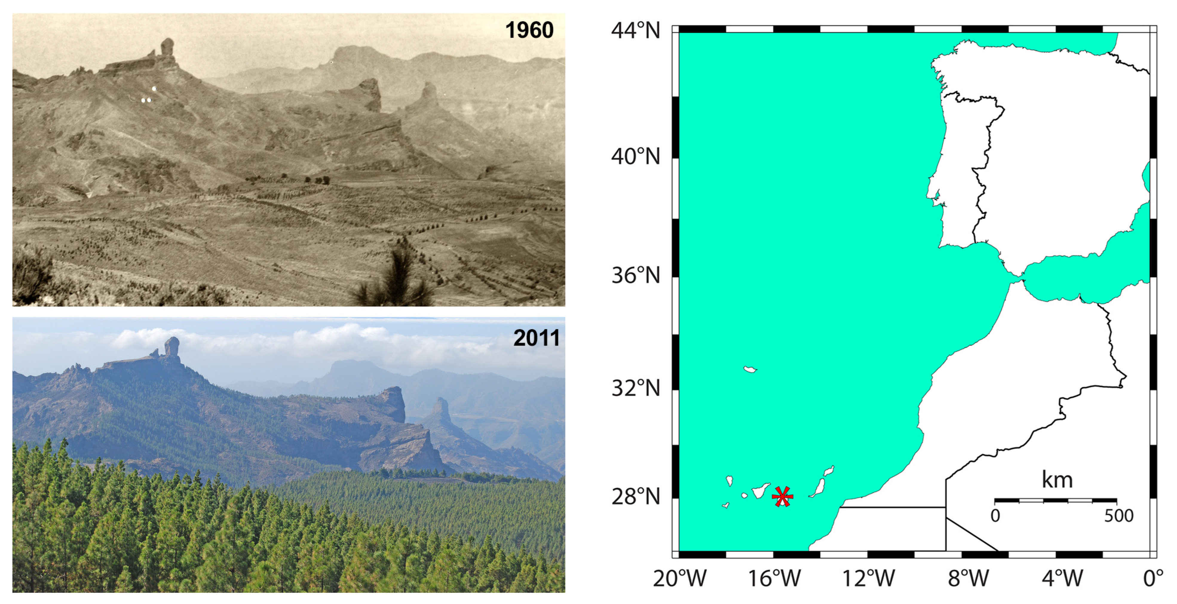
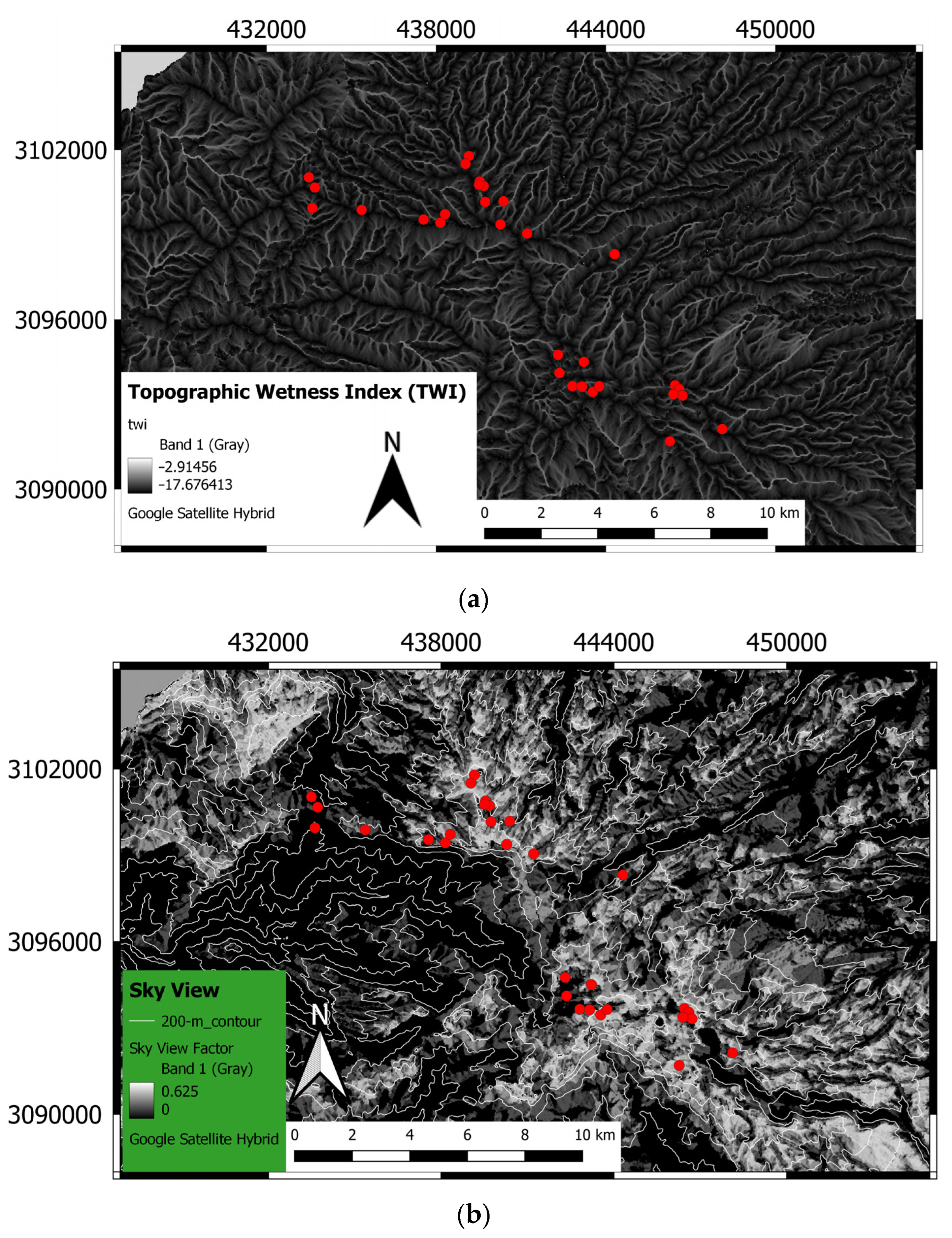
2.1. Study Area

Plantations of Pinus canariensis have been established since the 1950s throughout the species range in Gran Canaria (Canary Islands, Spain; Figure 1), and some stands were thinned in the late 1990s. Our 30 sample plots were located to capture the variability of terrain topography in plantations that had been thinned in 1995–1998 (13 plots) or not (17 plots), and all plots were in areas without tree pests or diseases. Plots were chosen so that they were always more than 200 m from tracks or roads and more than 500 m from each other. By selecting 15 trees per plot, a total of 450 trees were measured and cored using standard tools to determine the extent of the heartwood.

The climate of the Canary Islands is characterized by cool trade winds and cold surface waters [42], which create moderately temperate conditions during the warm season on land, despite the low latitude of the islands (~28° N). In winter, the Azores anticyclone changes location, and the frequency of trade wind days decreases to about half of the total [43]. Large-scale climatic processes are translated into precipitation and temperature regimes on land that are heavily influenced by topography, especially elevation and exposure [43]. Overall, precipitation increases and air temperature decreases at higher elevations and on slopes directly exposed to north-easterly trade winds [44]. Monthly average total precipitation and mean air temperature for a representative station (Figure S3) demonstrate limited seasonal differences in temperature, with August being the warmest month (mean of 21.1 °C) and January–February the coolest ones (mean of 12.4 °C).

Wet conditions are confined to the winter season (December–February), with monthly total precipitation being highest in December (38 mm) and lowest in June–August (6 mm per month). Annual averages are 16.5 °C for mean air temperature and 245 mm for total precipitation. According to recently interpolated graphics produced by the Consejo Insular de Aguas de Gran Canaria, maximum average annual rainfall in the island of Gran Canaria reaches 950 mm in areas where trade winds interact with topography to generate an almost continuous presence of clouds (“mar de nubes”; http://www.aguasgrancanaria.com/cartografia/tematica/precipitaciones.php, accessed on 2 August 2023).

2.2. Field and Laboratory Measurements

Field measurements and samples were collected in 2001 (Figure S4). Once a tree was chosen as the center of a plot, the 14 trees closest to it were identified. The height of these 15 trees was measured with a double-needle hypsometer (precision of 0.25 m), their stem was measured with a diameter tape (precision of 0.5 cm), and bark thickness was measured with an appropriate caliper (precision of 1 mm). A wood increment core was extracted at breast height (~1.3 m from the ground) on the north-facing side of each tree using a 40 cm Pressler borer. Existing information indicates that heartwood formation in Pinus canariensis is fairly uniform around the stem (Figures S1 and S2); hence, coring maximized the number of sampled trees without having to consider the core azimuth. Terrain slope and exposure were measured at the plot center, whose geographical coordinates were obtained using a GPS device. After measuring and coring the first 15 trees, the next 15 trees closest to the plot center were identified. The linear distance (m) from the plot center to tree 15 (D₁₅) and tree 30 (D₃₀), i.e., the furthest of the first 15 and the furthest of the last 15 trees, were measured and used to calculate a stand density index as follows [45]:

$$\frac{\mathrm{10,000}}{2\pi }\left(\frac{15}{D_{15}^2}+\frac{30}{D_{30}^2}\right)$$

(1)

where 10,000 is a conversion factor to express density as number of trees per hectare.

In the laboratory, the wood increment cores were analyzed to obtain the number of rings and the extent of the heartwood. When the core did not include the stem pith, its location was approximated using predetermined concentric circles [46], and the number of rings between the pith and the beginning of the core was then estimated using the average size of the innermost rings (Figure S5). Visible (and estimated) rings were used to calculate cambial stem age. Cumulated ring widths were used to reconstruct stem radii at five-year intervals (R5, R10, R15, R20, ...) with a precision of 0.5 cm. The heartwood radius and the stem radius inside the bark were also measured on each core. We followed [40]’s statement that “The sapwood–heartwood boundary is sharply defined by heartwood colour in Pinus canariensis. Noncoloured heartwood is absent in this species, and thus, all heartwood traits refer to coloured heartwood.”

2.3. Data Processing and Statistical Model

Because climate data were not available for the actual plot locations, we used topographical features to estimate indices of site moisture and insolation. A 30 m digital elevation model (DEM) was obtained using the OpenTopography DEM downloader plugin of QGIS [47] and used to produce a map of topographic wetness index (TWI) and a map of the Sky View factor. TWI is an index of where water will accumulate as a function of terrain slope and of the upstream contributing area [48]. Topographic variables (elevation, slope, and exposure, also in relation to the surrounding terrain) were further integrated into a Sky View factor, which varies from 1 for completely unobstructed land surfaces (such as horizontal surfaces or peaks and ridges) to 0 for completely obstructed land surfaces [49].

Frequency histograms, box plots, dot charts, and pairwise sample correlations (both Pearson’s and Spearman’s) were used for exploratory data analysis and to investigate relationships among plot and tree variables [50]. Whenever possible, relationships were examined by plot as well as for the entire dataset. As geographical coordinates were only available for the plot center, spatial autocorrelation of tree variables was geostatistically estimated [51,52] for the whole dataset by assigning the same location to all trees within a plot. The maximum pairwise Euclidean distance between the 30 plots was 17.1 km; 700 m distance intervals were used for variogram estimation and modeling because those intervals included more than 10 paired distances up to ~13 km.

The statistical relationship between the “tea” radius and other measured variables was estimated using a generalized linear mixed model (GLMM; [53,54,55]). To account for the presence of nested data, i.e., the tree measurements that were taken within each plot, we used a random effect for the sampled plot and a fixed effect for the tree stem diameter, with an interaction with the plot that allowed both a random intercept and a random slope so that the “tea”–diameter relationship could change from place to place. The potential influence of additional tree variables was tested by adding them as fixed terms, one at a time, to this initial GLMM and then comparing the model formulations using the Akaike information criterion (AIC; [56]). Spatial autocorrelation was modeled by an exponential covariance structure, and each GLMM was fit using restricted maximum likelihood estimation (REML; [57]).

Pine heartwood was often absent; hence, the “tea” radius (Rtea) was characterized by a large frequency of zero values. Because no data transformation can ameliorate this issue, we also used a binary response (1 for Rtea >0, and 0 otherwise) in order to apply mixed-effects logistic regression [58]. Introducing a random effect for plot location into the standard logistic regression model [59] generates a mixed-effects logistic regression. The advantage of a random intercept model is that the probability of a tree having “tea” is correlated to other trees on the same plot. It is worth noting that there is no random slope in this model, and that the predictor (diameter) is a continuous, but truncated, variable because it cannot be <0. Because of this, prior to model fitting, the diameter was “centered”, i.e., transformed into deviations from the mean [57]; otherwise, the intercept would represent the probability that a tree stem of zero diameter had “tea”, even though there cannot be a stem of zero diameter. By centering the stem diameter, the intercept acquired the more meaningful interpretation of the probability that a tree of average diameter had “tea”. All numerical analyses were performed in the R computing environment [60]. The mixed-effects models were fit using packages nlme [61], glmmML [62], and MASS [63].

3. Results

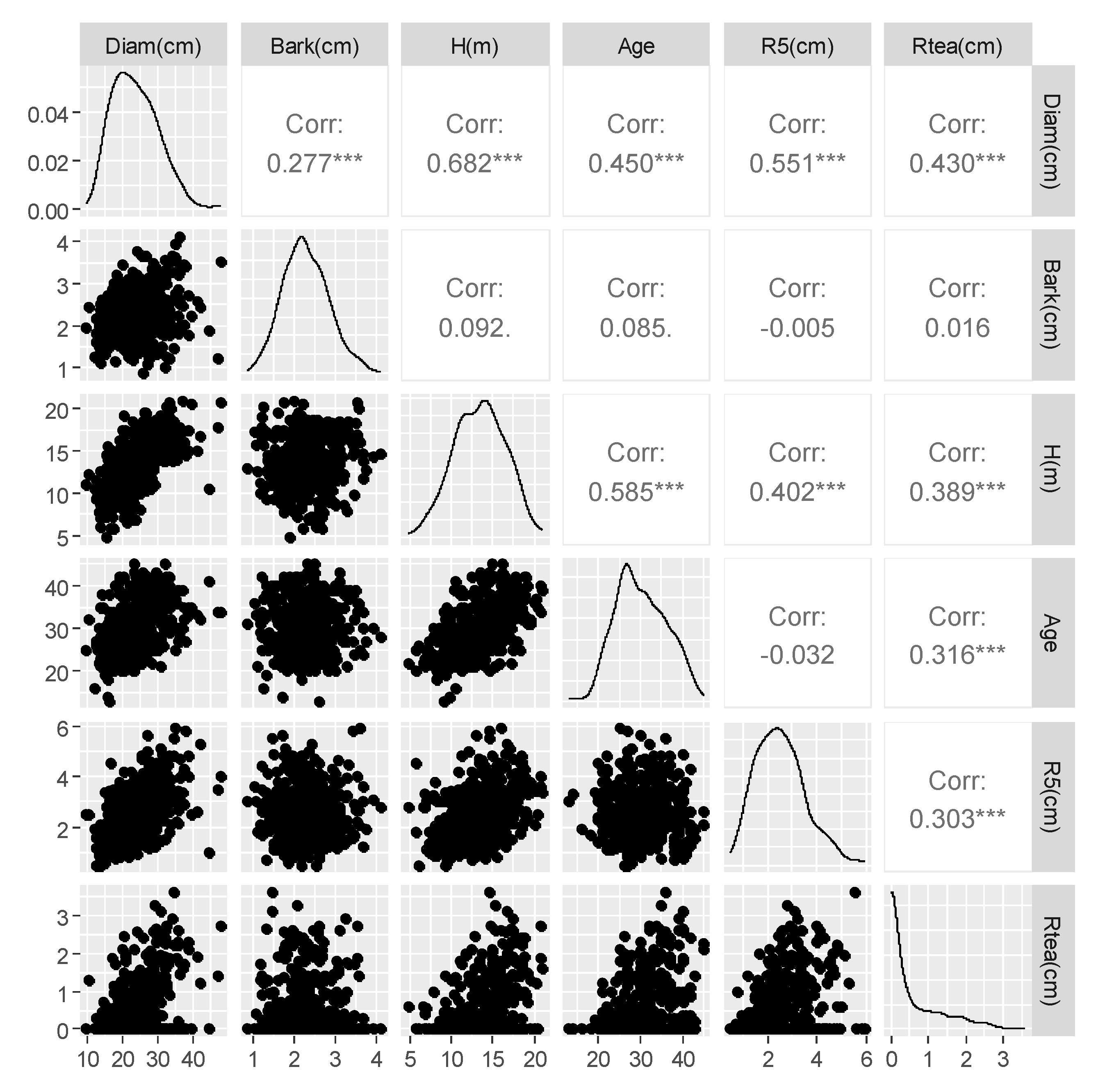
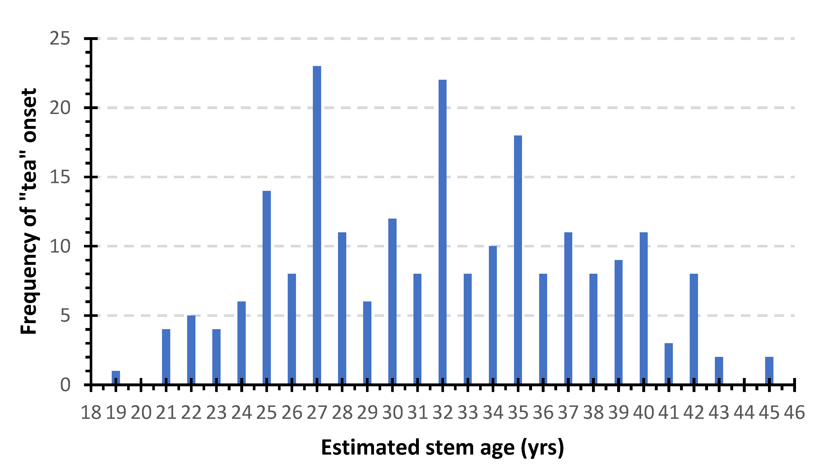
3.1. Sampled Trees and Exploratory Data Analysis

Sampled plots (Table S1, Figure 2) were distributed over an 880 m elevation interval, from 995 to 1875 m above mean sea level. Both thinned (13) and unthinned (17) plots were characterized by terrain that varied from almost flat (4%–9% slope) to steep (60%–70% slope), with different exposures. The map of TWI (Figure 2a) was plotted using a pseudo-color scheme, but it should be noted that because of the limited rainfall, there are no rivers in the island of Gran Canaria, only continuous streams in three of the island’s ravines.

Stand density showed a very large outlier for one of the plots (Table S1), which was considered to be correct, but its influence on correlations was reduced by log-transforming (natural logs) these indices. Because the original plot numbers were found to be inversely correlated with elevation and with the “easting” coordinate (X_UTM, Table S1) but directly correlated with the “northing” coordinate (Y_UTM, Table S1), such geographical dependencies were eliminated by reassigning plot numbers at random in subsequent analyses.

Tree-level variables showed reasonably bell-shaped frequency distributions with the exception of heartwood radius (Rtea; Figure 3 and Figure S6), which was highly skewed because of a large number of zeros, i.e., stems where heartwood could not be identified. Stem age for “tea” onset varied, with the earliest presence estimated at cambial ages of 19 years (Figure 4).

Among tree-level variables, stem diameter was the best predictor of heartwood radius (Figure 3 and Figure S6). Additional significant correlations between Rtea and other tree-level variables were most likely influenced by their collinearity with stem diameter (Figure 3 and Figure S6). Some spatial autocorrelation in heartwood radius was suggested by the variogram model (Figure S7).

3.2. Mixed-Effect Models

The generalized linear mixed model (GLMM), which was estimated with the nlme R package using restricted maximum likelihood estimation (REML), included both a random intercept and a random slope to account for plot-related differences in the relationship between tree stem diameter and “tea”. It also included an exponential covariance structure to account for spatial autocorrelation in the “tea”. Based on the model output (Table S2a, Figure 5), the fixed effects, i.e., the intercept and slope for the relationship between the stem diameter and the “tea” radius, were highly significant (p-value « 0). A high negative correlation (−0.969) existed between the random intercepts and slopes. The Akaike information criterion (AIC) of this model (884; Table S2a) was slightly higher than the AIC for the GLMM without spatially autocorrelated errors (880; detailed results for that model are not included).

After centering the stem diameter, a mixed-effects logistic regression model was fit to the data without any error covariance structure. The R package glmmML, which estimated the model parameters by maximum likelihood (Table S2b), showed that this model had a much lower AIC (571), thereby suggesting that the relationship between stem diameter and hardwood radius was more effectively modeled using the presence/absence of the “tea” rather than its measured size. Based on the model output (Table S2b), the probability (p) that the stem of pine j on plot i had “tea” is given by

logit(p_ij) = −0.038 + 0.089 diam_ij + a_i

with a_i ∼ N(0, 0.976²).

Because the random intercept a_i was assumed to be normally distributed with mean 0 and variance 0.976², 95% of a_i values would be between −1.96 × 0.976 and 1.96 × 0.976, which resulted in the 95% confidence interval of (−1.913, 1.913). GLMM-predicted probabilities of “tea” presence with respect to (centered) stem diameter for pines at all plots are shown graphically in Figure 6 using the logistic curves for a “typical” plot and for the upper and lower limits of this 95% confidence interval.

Based on the model results, going to a typical plot and sampling a pine of average stem diameter (the 0 value on the x-axis of Figure 6), the probability of finding “tea” would be ~0.49, which is the y-axis value obtained from the population curve (thick red line in Figure 6). Therefore, there is essentially a 50–50 chance of finding “tea” on an average pine sampled on a typical plot. In addition, for 95% of plots, this probability can be anything between 0.12 and 0.87 (i.e., the y-axis values obtained from the thin red lines in Figure 6), pointing to a large degree of inter-site variation.

Further Testing of Fixed Effects

Further statistical testing focused on other potential predictors of stem heartwood radius. Briefly, no other fixed effect appeared to contribute significantly to the predictive power of the mixed-effects logistic regression model shown earlier, and we report here two examples of those additional analyses. First, we investigated the impact of thinning by adding a categorical dummy variable (either 0 or 1) as a second fixed effect, together with its interaction with the stem diameter. Based on the p-values, the treatment and its interaction with stem diameter were not significant (p-value > 0.4), either in the GLMM with spatial autocorrelation (Table S2c) or in the logistic GLMM (not shown).

The second example reported here deals with the tree initial radial growth rate, represented by the cumulated size of the first five annual rings (R5 in Figure 3 and Figure S6). As shown by smoothed scatterplots (red lines in Figure S6), this variable was positively correlated with stem diameter (linearly), height (nonlinearly), and the size of the heartwood (slightly). The (centered) R5 had a negative and barely significant (p-value = 0.0397) coefficient in the logistic GLMM (not shown), but its interaction with the stem diameter was not significant (p-value = 0.665). The mixed-effects logistic regression model was, however, slightly improved by adding this second fixed term, as shown by a minimally lower AIC (569.8). Because the interaction term was not significant, the model was refitted without it, and the AIC decreased a bit more (568; Table S2d). Because the output from the glmmML package did not include the estimated correlations between fixed effects, we used the glmmPQL function from the MASS package to obtain that information (Table S2e). The interaction term between the two fixed effects was confirmed to be nonsignificant (results not shown); hence, the model was refit without the interaction, and a high negative correlation (−0.607) was found between the two fixed effects, i.e. stem diameter and five-year cumulative growth.

Based on the model output (Table S2e), the probability (p) that the stem of pine j on plot i had “tea” is given by

logit(p_ij) = −0.033 + 0.122 diam_ij − 0.344 R5_ij + a_i

(2)

with a_i ∼ N(0, 1.034²).

A graphical representation of GLMM-predicted probabilities that pine j on plot i had “tea” would require a 3D plot to include the “stem diameter anomaly” axis (Figure 6) as well as the new “R5 anomaly” axis. In addition, one can derive from the logit equation that there is still essentially a 50–50 chance of finding “tea” on an average pine sampled on a typical plot, with 95% of plots having probability between 0.11 and 0.88. Overall, introducing the R5 variable as a fixed effect improved the model relatively little, even though measuring R5 requires considerable extra effort both in the field (to collect increment cores) and in the laboratory (to analyze growth rings).

4. Discussion

In our study, the presence of heartwood or “tea” in Pinus canariensis stands that were planted in the island of Gran Canaria was most efficiently predicted by stem diameter measured at breast height. Based on the GLMM with exponential error covariance structure, some spatial autocorrelation occurred up to a linear distance of about 500 m, but there was no statistical advantage for including this model component. In other words, a random slope and intercept of the DBH–“tea” relationship already accounted for most of the spatially related variability in heartwood radius. Furthermore, the GLMM model became more effective when the relationship between stem diameter and heartwood was modeled using the presence/absence of the “tea” rather than its measured size.

Stem diameter was also the best estimator of heartwood radius for seven Chinese species in temperate climates [64]. The connection between heartwood formation and tree diameter was found to be stronger than the one with age in other species too, including Tectona grandis [65], Acacia melanoxylon R. Br. [66], and Eucalyptus globulus Labill. [67]. However, stem age was found by other authors to predict the amount of heartwood in Pinus canariensis [40,68] and in other species [16,27,28]. As the maximum estimated tree age at our study plots was 46 years (Figure 4), which is quite low due to the artificial regeneration of these stands, it is possible that the relationship between stem age and “tea” was masked by the connection between stem age and size, which is usually stronger at younger ages.

It should be noted that the onset of “tea” formation was found to be at about 30 years of age in naturally regenerated stands of Canary Island pine [40,68], whereas in the sampled plantations, it was about 2/3 of that at ~19 years (Figure 4). The earlier appearance of “tea” in these artificial stands could be linked to lower competition for resources because of understory removal at the time of planting and fairly regular spacing among pines. Pinus canariensis is a shade-intolerant species; hence, its natural regeneration occurs mostly after disturbances, such as wildfires or tree falls, which open forest gaps where regeneration is abundant, and growth is then slowed down by competitive interactions.

Initial stem growth, when cambial age is low, has been found to have a positive influence on the development of heartwood in natural stands of Pinus canariensis [35] and Pinus radiata [41,69]. In our study, cumulated wood increments during the first five years of cambial age (the “R5” variable), while statistically significant, added comparatively little to the performance of the GLMM. Furthermore, the sign of the fixed-effect coefficient for R5 was negative, which is the opposite of what was observed in previous studies. While we cannot exclude a numerical artifact caused by computational instabilities that are inevitable under collinearity of predictors [57,70], it is conceivable that larger tree rings would imply larger cell lumens, which in turn could favor sap flow, prevent lumen occlusion, and thereby delay the formation of heartwood. Future research should be aimed at investigating chemical and anatomical characteristics of Pinus canariensis heartwood to test such an intriguing hypothesis.

The lack of a significant difference in the relationship between stem diameter and heartwood formation between plots that were thinned and those that were not may be linked to several factors. It is interesting to note that a similar lack of reaction to pruning was reported for Pinus sylvestris [71], which experienced a negative defoliation impact in terms of stem growth rates but no significant connection to heartwood size. Because heartwood formation was not favored by thinning and firewood obtained from intermediate silvicultural treatments of Canary Island pine has no economic value, our study suggests that reforestation should be carried out at final densities or close to them so that thinning is not necessary.

While we estimated climatic conditions at the sampled plots using topographically derived variables, and found no significant correlations, other studies have indicated that climate can influence heartwood formation in both conifers [72,73] and angiosperms [74]. For teak (Tectona grandis) grown in India, wet sites yielded larger heartwood than dry sites [75], whereas the opposite case was found for teak planted in Ghana [76]. In the boreal forest, black spruce (Picea mariana (Mill.) BSP) heartwood was greater under wet conditions than under dry ones [77], whereas in natural stands of Pinus canariensis, humid climates corresponded to lower amounts of heartwood than dry climates [40]. Future research should further test the impact of climatic variability on heartwood formation because there is a possibility that our sampled plots were located in areas with higher moisture compared to the entire range of climatic conditions that are naturally experienced by Pinus canariensis in its native habitat.

The heartwood (“tea”) of Pinus canariensis has been used for economic and cultural activities as a highly prized material because of its color, density, and durability. There is archeological evidence that even pre-Hispanic societies used “tea” for constructing barns and for funeral practices [78]. Intensive exploitation of the pine forest in the Canary Islands started in the 15^th century with Spanish colonization as quality wood was required to build furniture and ships and very large pines were present in the islands, most likely exceeding the height and diameter of any currently remaining pine [35].

The percentage of heartwood in mature trees is an essential characteristic for both wood quality and carbon sequestration [79]. Carbon absorbed from the atmosphere is deposited for a long time in the living tissue of woody plants, but there are differences in carbon amounts between heartwood and sapwood, which are usually inconsistent between species and within taxonomic groups [80]. As carbon stocks in forest ecosystems play a fundamental role in global management of natural resources in a changing world [81,82], future research should then be aimed at clarifying the factors that control heartwood formation in this species as well as others with the goal of designing the most carbon-conscious forest policies.

References

1. International Association of Wood Anatomists (IAWA). Multilingual Glossary of Terms used in Wood Anatomy; Verlagsanstalt Buchdruckere: Winterthur, Switzerland, 1964; Volume 40, p. 26. [Google Scholar]
2. Hillis, W.E. Heartwood and Tree Exudates; Springer: Berlin, Germany, 1987; p. 268. [Google Scholar]
3. Beekwilder, J.; van Houwelingen, A.; Cankar, K.; van Dijk, A.D.J.; de Jong, R.M.; Stoopen, G.; Bouwmeester, H.; Achkar, J.; Sonke, T.; Bosch, D. Valencene synthase from the heartwood of Nootka cypress (Callitropsis nootkatensis) for biotechnological production of valencene. Plant Biotechnol. J. 2014, 12, 174–182. [Google Scholar] [CrossRef] [PubMed]
4. Celedon, J.M.; Chiang, A.; Yuen, M.M.S.; Diaz-Chavez, M.L.; Madilao, L.L.; Finnegan, P.M.; Barbour, E.L.; Bohlmann, J. Heartwood-specific transcriptome and metabolite signatures of tropical sandalwood (Santalum album) reveal the final step of (Z)-santalol fragrance biosynthesis. Plant J. 2016, 86, 289–299. [Google Scholar] [CrossRef] [PubMed]
5. Taylor, A.M.; Gartner, B.L.; Morrell, J.J. Heartwood formation and natural durability—A review. Wood Fiber. Sci. 2002, 34, 587–611. [Google Scholar]
6. Galibina, N.A.; Moshnikov, S.A.; Nikerova, K.M.; Afoshin, N.V.; Ershova, M.A.; Ivanova, D.S.; Kharitonov, V.A.; Romashkin, I.V.; Semenova, L.I.; Serkova, A.A.; et al. Changes in the intensity of heartwood formation in Scots pine (Pinus sylvestris L.) ontogenesis. IAWA J. 2022, 43, 299–321. [Google Scholar] [CrossRef]
7. Bamber, R.K. Sapwood and Heartwood; Forestry Commission of New South Wales: Beecroft, Australia, 1987; p. 7. [Google Scholar]
8. Ekeberg, D.; Flæte, P.-O.; Eikenes, M.; Fongen, M.; Naess-Andresen, C.F. Qualitative and quantitative determination of extractives in heartwood of Scots pine (Pinus sylvestris L.) by gas chromatography. J. Chromatogr. A 2006, 1109, 267–272. [Google Scholar] [CrossRef]
9. Petit, G.; Mencuccini, M.; Carrer, M.; Prendin, A.L.; Hölttä, T. Axial conduit widening, tree height and height growth rate set the hydraulic transition of sapwood into heartwood. J. Exp. Bot. 2023, erad227. [Google Scholar] [CrossRef]
10. Beauchamp, K.; Mencuccini, M.; Perks, M.; Gardiner, B. The regulation of sapwood area, water transport and heartwood formation in Sitka spruce. Plant Ecol. Divers. 2013, 6, 45–56. [Google Scholar] [CrossRef]
11. Spicer, R. Senescence in secondary xylem: Heartwood formation as an active developmental program. In Vascular Transport in Plants; Holbrook, N.M., Zwieniecki, M.A., Eds.; Elsevier Academic Press: San Diego, CA, USA, 2005; pp. 457–475. [Google Scholar]
12. Frey-Wyssling, A.; Bosshard, H.H. Cytology of the ray cells in sapwood and heartwood. Holzforschung 1959, 13, 129–137. [Google Scholar] [CrossRef]
13. Stewart, C.M. Excretion and heartwood formation in living trees. Science 1966, 153, 1068–1074. [Google Scholar] [CrossRef]
14. Carrodus, B.B. Carbon dioxide and the formation of heartwood. New Phytol. 1971, 70, 939–943. [Google Scholar] [CrossRef]
15. Shain, L.; Mackay, J. Seasonal fluctuation in respiration of aging xylem in relation to heartwood formation in Pinus radiata. Can. J. Bot. 1973, 51, 737–741. [Google Scholar] [CrossRef]
16. Bamber, R.K. Heartwood, its function and formation. Wood Sci.Technol. 1976, 10, 1–8. [Google Scholar] [CrossRef]
17. Fries, A.; Ericsson, T. Genetic parameters in diallel-crossed Scots pine favor heartwood formation breeding objectives. Can. J. For. Res. 1998, 28, 937–941. [Google Scholar] [CrossRef]
18. Long, J.N.; Smith, F.W. Leaf area-sapwood area relations of lodgepole pine as influenced by stand density and site index. Can. J. For. Res. 1988, 18, 247–250. [Google Scholar] [CrossRef]
19. Rogers, R.; Hinckley, T. Foliar weight and area related to current sapwood area in oak. For. Sci. 1979, 25, 298–303. [Google Scholar]
20. Waring, R.; Gholz, H.; Grier, C.; Plummer, M. Evaluating stem conducting tissue as an estimator of leaf area in four woody angiosperms. Can. J. Bot. 2011, 55, 1474–1477. [Google Scholar] [CrossRef]
21. Shinozaki, K.; Yoda, K.; Hozumi, K.; Kira, T. A quantitative analysis of plant form-the pipe model theory: I. Basic analyses. Jpn. J. Ecol. 1964, 14, 97–105. [Google Scholar] [CrossRef]
22. Marchand, P.J. Sapwood area as an estimator of foliage biomass and projected leaf area for Abies balsamea and Picea rubens. Can. J. For. Res. 1984, 14, 85–87. [Google Scholar] [CrossRef]
23. Whitehead, D.; Edwards, W.R.N.; Jarvis, P.G. Conducting sapwood area, foliage area, and permeability in mature trees of Picea sitchensis and Pinus contorta. Can. J. For. Res. 1984, 14, 940–947. [Google Scholar] [CrossRef]
24. Waring, R.H.; Schroeder, P.E.; Oren, R. Application of the pipe model theory to predict canopy leaf area. Can. J. For. Res. 1982, 12, 556–560. [Google Scholar] [CrossRef]
25. Morataya, R.; Galloway, G.; Berninger, F.; Kanninen, M. Foliage biomass-sapwood (area and volume) relationships of Tectona grandis L.F. and Gmelina arborea Roxb.: Silvicultural implications. For. Ecol. Manag. 1999, 113, 231–239. [Google Scholar] [CrossRef]
26. Todorovski, S. Effect of certain factors on the proportion of sapwood and heartwood in the stem of Pinus sylvestris and Pinus nigra. For. Abstr. 1968, 2908. [Google Scholar]
27. Yang, K.C.; Hazenberg, G. Relationship between tree age and sapwood/heartwood width in Populus tremuloides Michx. Wood Fiber Sci. 1991, 23, 247–252. [Google Scholar]
28. Yang, K.C.; Hazenberg, G. Sapwood and heartwood width relationship to tree age in Pinus banksiana. Can. J. For. Res. 1991, 21, 521–525. [Google Scholar] [CrossRef]
29. Sellin, A. Sapwood amount in Picea abies (L.) Karst. determined by tree age and radial growth rate. Holzforschung 1996, 50, 291–296. [Google Scholar] [CrossRef]
30. Björklund, L. Identifying heartwood-rich stands or stems of Pinus sylvestris by using inventory data. Silva Fenn. 1999, 33, 611. [Google Scholar] [CrossRef]
31. Boanza, M.V.; Gutiérrez, A.; Grau, J.M. Variación de la densidad, la humedad, el duramen y la corteza con la altura en el tronco de pino laricio. In Proceedings of the III Congreso Forestal Español, Granada, Spain, 25–28 September 2001; p. 5. [Google Scholar]
32. Koch, P. Utilization of the Southern Pines—Volume 2; USDA-Forest Service, Southern Forest Experiment Station: Asheville, NC, USA, 1972; pp. 735–1663. [Google Scholar]
33. Knapic, S.; Pereira, H. Within-tree variation of heartwood and ring width in maritime pine (Pinus pinaster Ait.). For. Ecol. Manag. 2005, 210, 81–89. [Google Scholar] [CrossRef]
34. Moya, R.; Calvo-Alvarado, J. Variation of wood color parameters of Tectona grandis and its relationship with physical environmental factors. Ann. For. Sci. 2012, 69, 947–959. [Google Scholar] [CrossRef]
35. Climent, J.; Gil, L.; Pardos, J. Heartwood and sapwood development and its relationship to growth and environment in Pinus canariensis Chr.Sm ex DC. For. Ecol. Manag. 1993, 59, 165–174. [Google Scholar] [CrossRef]
36. Córdoba, L.C.; de Medina, F.O.F. Estudio Sobre la Vegetación y Flora Forestal de las Canarias Occidentales; Ministerio de Agricultura, Dirección General de Montes, Caza y Pesca Fluvial, Instituto Forestal de Investigaciones y Experiencias: Madrid, Spain, 1951; p. 465. [Google Scholar]
37. Parsons, J.J. Human influences on the pine and laurel forests of the Canary Islands. Geogr. Rev. 1981, 71, 253–271. [Google Scholar] [CrossRef]
38. Arévalo, J.R.; Fernández-Palacios, J.M. 9550-Pinares endémicos canarios. In Bases Ecológicas Preliminares Para la Conservación de los Tipos de Hábitat de Interés Comunitario en España; Dirección General de Medio Natural y Política Forestal, Ministerio de Medio Ambiente y Medio Rural y Marino: Madrid, Spain, 2009; p. 74. [Google Scholar]
39. Rodríguez, R.A.L. Diferenciación Adaptativa Entre Poblaciones de Pinus Canariensis Chr. Sm. ex DC. Ph.D. Thesis, Universidad Politécnica de Madrid, Madrid, Spain, 2009. [Google Scholar]
40. Climent, J.; Chambel, M.R.; Pérez, E.; Gil, L.; Pardos, J. Relationship between heartwood radius and early radial growth, tree age, and climate in Pinus canariensis. Can. J. For. Res. 2002, 32, 103–111. [Google Scholar] [CrossRef]
41. Wilkes, J. Heartwood development and its relationship to growth in Pinus radiata. Wood Sci.Technol. 1991, 25, 85–90. [Google Scholar] [CrossRef]
42. Arístegui, J.; Barton, E.D.; Álvarez-Salgado, X.A.; Santos, A.M.P.; Figueiras, F.G.; Kifani, S.; Hernández-León, S.; Mason, E.; Machú, E.; Demarcq, H. Sub-regional ecosystem variability in the Canary Current upwelling. Prog. Oceanog. 2009, 83, 33–48. [Google Scholar] [CrossRef]
43. del Arco Aguilar, M.J.; Delgado, O.R. Vegetation of the Canary Islands; Springer International Publishing: Cham, Switzerland, 2018; p. 429. [Google Scholar]
44. Puyol, D.G.; Herrera, R.G.; Martín, E.H.; Presa, L.G.; Rodríguez, P.R. Major influences on precipitation in the Canary Islands. In Climatic Change: Implications for the Hydrological Cycle and for Water Management; Beniston, M., Ed.; Springer: Dordrecht, The Netherlands, 2002; pp. 57–73. [Google Scholar]
45. García, M.B. Manual de Dasometría; Organismo Autónomo Parques Nacionales: Madrid, Spain, 2011; p. 135. [Google Scholar]
46. Applequist, M.B. A simple pith locator for use with off center increment cores. J. For. Res. 1958, 56, 141. [Google Scholar]
47. QGIS.org. QGIS Geographic Information System; 3.28.4-Firenze; QGIS Association: Florence, Italy, 2022. [Google Scholar]
48. Kopecký, M.; Macek, M.; Wild, J. Topographic Wetness Index calculation guidelines based on measured soil moisture and plant species composition. Sci. Total Environ. 2021, 757, 143785. [Google Scholar] [CrossRef]
49. Böhner, J.; Antonić, O. Land-surface parameters specific to topo-climatology. In Developments in Soil Science; Hengl, T., Reuter, H.I., Eds.; Elsevier: Amsterdam, The Netherlands, 2009; Volume 33, pp. 195–226. [Google Scholar]
50. Sokal, R.R.; Rohlf, F.J. Biometry, 4th ed.; W.H. Freeman and Co.: New York, NY, USA, 2012; p. 937. [Google Scholar]
51. Isaaks, E.H.; Srivastava, R.M. An Introduction to Applied Geostatistics; Oxford University Press: New York, NY, USA, 1989. [Google Scholar]
52. Biondi, F.; Myers, D.E.; Avery, C.C. Geostatistically modeling stem size and increment in an old-growth forest. Can. J. For. Res. 1994, 24, 1354–1368. [Google Scholar] [CrossRef]
53. Venables, W.N.; Dichmont, C.M. GLMs, GAMs and GLMMs: An overview of theory for applications in fisheries research. Fish. Res. 2004, 70, 319–337. [Google Scholar] [CrossRef]
54. Bolker, B.M.; Brooks, M.E.; Clark, C.J.; Geange, S.W.; Poulsen, J.R.; Stevens, M.H.H.; White, J.-S.S. Generalized linear mixed models: A practical guide for ecology and evolution. Trends Ecol. Evol. 2009, 24, 127–135. [Google Scholar] [CrossRef]
55. Venables, W.N.; Ripley, B.D. Modern Applied Statistics with S, 4th ed.; Springer Science+Business Media: New York, NY, USA, 2002; p. 495. [Google Scholar]
56. Akaike, H. A new look at the statistical model identification. IEEE Trans. Automat. Contr. 1974, 19, 716–723. [Google Scholar] [CrossRef]
57. Zuur, A.F.; Ieno, E.N.; Walker, N.J.; Saveliev, A.A.; Smith, G.M. Mixed Effects Models and Extensions in Ecology with R; Springer Science+Business Media: New York, NY, USA, 2009; p. 574. [Google Scholar]
58. Gelman, A.; Hill, J. Data Analysis Using Regression and Multilevel/Hierarchical Models; Cambridge University Press: Cambridge, UK, 2006. [Google Scholar]
59. Hosmer, D.W., Jr.; Lemeshow, S.; Sturdivant, R.X. Applied Logistic Regression; John Wiley & Sons, Inc.: Hoboken, NJ, USA, 2013. [Google Scholar]
60. R Core Team. R: A Language and Environment for Statistical Computing, 4.1.2; R Foundation for Statistical Computing: Vienna, Austria, 2021. [Google Scholar]
61. Pinheiro, J.; Bates, D.; DebRoy, S.; Sarkar, D.; Eispack, A.; Heisterkamp, S.; Van Willigen, B.; Ranke, J.; R Core Team. Package ‘nlme’: Linear and Nonlinear Mixed Effects Models; R Package Version 3.1-162; R Foundation for Statistical Computing: Vienna, Austria, 2023. [Google Scholar]
62. Broström, G.; Jin, J.; Holmberg, H. Package ‘glmmML’: Generalized Linear Models with Clustering; R Package Version 1.1.4; R Foundation for Statistical Computing: Vienna, Austria, 2022. [Google Scholar]
63. Ripley, B.D.; Venables, W.N.; Bates, D.M.; Hornik, K.; Gebhardt, A.; Firth, D. Package ‘MASS’: Support Functions and Datasets for Venables and Ripley’s MASS; R Package Version 7.3-60; R Foundation for Statistical Computing: Vienna, Austria, 2023. [Google Scholar]
64. Wang, X.; Wang, C.; Zhang, Q.; Quan, X. Heartwood and sapwood allometry of seven Chinese temperate tree species. Ann. For. Sci. 2010, 67, 410. [Google Scholar] [CrossRef]
65. Kokutse, A.D.; Baillères, H.; Stokes, A.; Kokou, K. Proportion and quality of heartwood in Togolese teak (Tectona grandis L.f.). For. Ecol. Manag. 2004, 189, 37–48. [Google Scholar] [CrossRef]
66. Knapic, S.; Tavares, F.; Pereira, H. Heartwood and sapwood variation in Acacia melanoxylon R. Br. trees in Portugal. Forestry 2006, 79, 371–380. [Google Scholar] [CrossRef]
67. Gominho, J.; Pereira, H. The influence of tree spacing in heartwood content in Eucalyptus globulus Labill. Wood Fiber Sci. 2005, 582–590. [Google Scholar]
68. Climent, J.; Chambel, M.R.; Gil, L.; Pardos, J.A. Vertical heartwood variation patterns and prediction of heartwood volume in Pinus canariensis Sm. For. Ecol. Manag. 2003, 174, 203–211. [Google Scholar] [CrossRef]
69. Hillis, W.E.; Ditchburne, N. The prediction of heartwood diameter in radiata pine trees. Can. J. For. Res. 1974, 4, 524–529. [Google Scholar] [CrossRef]
70. Graham, M.H. Confronting multicollinearity in ecological multiple regression. Ecology 2003, 84, 2809–2815. [Google Scholar] [CrossRef]
71. Bergström, B.; Gref, R.; Ericsson, A. Effects of pruning on heartwood formation in Scots pine trees. J. For. Sci. 2004, 50, 11–16. [Google Scholar] [CrossRef]
72. Jakubowski, M.; Kałuziński, D.; Tomczak, A.; Jelonek, T. Proportion of heartwood and sapwood in Scots pine (Pinus sylvestris L.) stems grown in different site conditions. Ann. WULS-SGGW For. Wood Technol. 2015, 92, 122–126. [Google Scholar]
73. Tarelkina, T.V.; Galibina, N.A.; Moshnikov, S.A.; Nikerova, K.M.; Moshkina, E.V.; Genikova, N.V. Anatomical and morphological features of Scots pine heartwood formation in two forest types in the middle taiga subzone. Forests 2022, 13, 17. [Google Scholar] [CrossRef]
74. Almeida, M.N.F.d.; Vidaurre, G.B.; Pezzopane, J.E.M.; Lousada, J.L.P.C.; Silva, M.E.C.M.; Câmara, A.P.; Rocha, S.M.G.; Oliveira, J.C.L.d.; Campoe, O.C.; Carneiro, R.L.; et al. Heartwood variation of Eucalyptus urophylla is influenced by climatic conditions. For. Ecol. Manag. 2020, 458, 117743. [Google Scholar] [CrossRef]
75. Pk, T.; Km, B. Log characteristics and sawn timber recovery of home-garden teak from wet and dry localities of Kerala, India. Small-Scale For. 2009, 8, 15–24. [Google Scholar] [CrossRef]
76. Amoah, M.; Inyong, S. Comparison of some physical, mechanical and anatomical properties of smallholder plantation teak (Tectona grandis Linn. f.) from dry and wet localities of Ghana. J. Indian Acad. Wood Sci. 2019, 16, 125–138. [Google Scholar] [CrossRef]
77. Krause, C.; Gagnon, R. The relationship between site and tree characteristics and the presence of wet heartwood in black spruce in the boreal forest of Quebec, Canada. Can. J. For. Res. 2011, 36, 1519–1526. [Google Scholar] [CrossRef]
78. Vidal-Matutano, P.; Delgado-Darias, T.; López-Dos Santos, N.; Henríquez-Valido, P.; Velasco-Vázquez, J.; Alberto-Barroso, V. Use of decayed wood for funerary practices: Archaeobotanical analysis of funerary wooden artefacts from Prehispanic (ca. 400–1500 CE) Gran Canaria (Canary Islands, Spain). Quatern. Int. 2021, 593, 384–398. [Google Scholar] [CrossRef]
79. Thurner, M.; Beer, C.; Crowther, T.; Falster, D.; Manzoni, S.; Prokushkin, A.; Schulze, E.-D. Sapwood biomass carbon in northern boreal and temperate forests. Glob. Ecol. Biogeogr. 2019, 28, 640–660. [Google Scholar] [CrossRef]
80. Lamlom, S.; Savidge, R. A reassessment of carbon content in wood: Variation within and between 41 North American species. Biomass Bioenerg. 2003, 25, 381–388. [Google Scholar] [CrossRef]
81. Roebroek, C.T.J.; Duveiller, G.; Seneviratne, S.I.; Davin, E.L.; Cescatti, A. Releasing global forests from human management: How much more carbon could be stored? Science 2023, 380, 749–753. [Google Scholar] [CrossRef]
82. Terrer, C.; Phillips, R.P.; Hungate, B.A.; Rosende, J.; Pett-Ridge, J.; Craig, M.E.; van Groenigen, K.J.; Keenan, T.F.; Sulman, B.N.; Stocker, B.D.; et al. A trade-off between plant and soil carbon storage under elevated CO2. Nature 2021, 591, 599–603. [Google Scholar] [CrossRef]
83. Climate-Data.org. TEJEDA CLIMATE (SPAIN): Data and Graphs for Weather & Climate. Available online: https://en.climate-data.org/europe/spain/canary-islands/tejeda-199883/ (accessed on 5 March 2023).
Figure 1. Repeated photographs of the “Monumento natural del Roque Nublo”, Gran Canaria, Spain (the island location is shown by a red asterisk in the map on the right), showing the effective reforestation between 1960 and 2011 obtained by planting the endemic Pinus canariensis (photo credit: Fondo para la Etnografía y el Desarrollo de la Artesanía Canaria—FEDAC).
Forests 14 01719 g001
Figure 2. Map of the study area showing plot locations (solid red dots). Universal Transverse Mercator (UTM, zone 28N) coordinates at 6 km intervals are displayed on the left y-axis (“northing”) and on the top x-axis (“easting”). A 30 m digital elevation model (DEM) was used to calculate (a) the topographic wetness index (TWI) and (b) the Sky View factor with elevation contour lines at 200 m intervals.
Forests 14 01719 g002
Figure 3. Paired sample linear correlations (Pearson’s) between selected tree variables (see Figure S6 for variable names). Smoothed frequency histograms are plotted on the diagonal, with paired scatterplots (black dots) below the diagonal and correlation values (*** = p-value < 0.001) above it.
Forests 14 01719 g003
Figure 4. Estimated stem age when heartwood could first be identified on 222 out of the 450 sampled pines.
Forests 14 01719 g004
Figure 5. Relationship between stem size and heartwood radius in Pinus canariensis plantations. The thick black line is the stem diameter–“tea” relationship on a typical plot as linear regression parameters in the GLMM were estimated with respect to an individual plot (thin black lines) due to the random intercept and slope (see text for details).
Forests 14 01719 g005
Figure 6. Logistic curves showing the estimated probabilities of “tea” presence for a range of stem diameter anomalies (= centered values). The thick red line in the middle corresponds to a typical plot, i.e., the predicted probability for the “population of locations”, or ai = 0. The other two red lines are obtained by adding and subtracting 1.913 from the random intercept to the predictor function. Hence, 95% of the plots have logistic curves between these two extremes, and the space between these two curves represents the variation of predicted values per plot.
Forests 14 01719 g006
Disclaimer/Publisher’s Note: The statements, opinions and data contained in all publications are solely those of the individual author(s) and contributor(s) and not of MDPI and/or the editor(s). MDPI and/or the editor(s) disclaim responsibility for any injury to people or property resulting from any ideas, methods, instructions or products referred to in the content.