Abstract
Mangroves have important roles in regulating climate change, and in reducing the impact of wind and waves. Analysis of the chlorophyll content of mangroves is important for monitoring their health, and their conservation and management. Thus, this study aimed to apply four regression models, eXtreme Gradient Boosting (XGBoost), Random Forest (RF), Partial Least Squares (PLS) and Adaptive Boosting (AdaBoost), to study the inversion of Soil Plant Analysis Development (SPAD) values obtained from near-ground hyperspectral data of three dominant species, Bruguiera sexangula (Lour.) Poir. (B. sexangula), Ceriops tagal (Perr.) C. B. Rob. (C. tagal) and Rhizophora apiculata Blume (R. apiculata) in Qinglan Port Mangrove Nature Reserve. The accuracy of the model was evaluated using R2, RMSE, and MAE. The mean SPAD values of R. apiculata (SPADavg = 66.57), with a smaller dispersion (coefficient of variation of 6.59%), were higher than those of C. tagal (SPADavg = 61.56) and B. sexangula (SPADavg = 58.60). The first-order differential transformation of the spectral data improved the accuracy of the prediction model; R2 was mostly distributed in the interval of 0.4 to 0.8. The accuracy of the XGBoost model was less affected by species differences with the best stability, with RMSE at approximately 3.5 and MAE at approximately 2.85. This study provides a technical reference for large-scale detection and management of mangroves.
1. Introduction
Mangrove forests are a special type of coastal ecosystem in the transition zone between terrestrial and marine ecosystems [1,2]. They are a complex-structured salt-tolerant wetland ecological community composed of woody plants, such as evergreen shrubs and trees, with mangrove plants as the mainstay. These plants can tolerate extreme environments such as high salinity, high temperature, flooding, and poor soils, and are important for shoreline protection. They play a role in slowing coastal erosion, provide resiliency to natural disasters such as storms and help protect agricultural land [3,4]. Mangrove plants provide habitats and breeding sites for many marine animals and are an important component in maintaining ecological balance. Mangroves have high socioeconomic value [5], but over-exploitation and human activities have threatened growth in mangrove forests and there has been a significant reduction in mangrove area [6,7,8]. In recent years, there has been an increasing awareness of the need to protect mangrove ecosystems, and many mangrove conservation and restoration efforts have been made [9,10] to ensure the sustainable development of mangrove ecosystems.
Chlorophyll is an important chemical in plants that is involved in both photosynthesis and growth and development [11]. Chlorophyll content is a key indicator that enables effective monitoring of plant health and overall growth. The traditional method for measuring chlorophyll content is chemical analysis in the laboratory, which is time consuming and costly, although the accuracy of the measurement is high [12,13]. Many studies have shown a strong correlation between chlorophyll content and Soil and Plant Analysis Development (SPAD) values, which are typically measured with a convenient handheld meter that does not destroy plant tissue [14]. Brown et al., (2022) demonstrated that SPAD measurements can be used to represent leaf chlorophyll content in forests under calibrated conditions [15]. In mangrove studies conducted as early as 1997, Connelly reported a large correlation (R2 > 0.6) between the chlorophyll content of mangroves and SPAD-502 readings [16]. Neres et al., (2020) also demonstrated that chlorophyll concentration indices of SPAD-502 and those of mangroves can be inter-converted [17]. Therefore, SPAD can be used to represent the leaf chlorophyll content of mangrove plants. The determination of the SPAD values of mangrove plant leaves might be expected to be effective in indicating the health status of mangrove plants and provide a basis for decision making in the monitoring and management of mangroves.
Accurate leaf SPAD values can be obtained through field measurements; however, the complex growth environment of mangroves makes field experiments less accessible, and only the SPAD measurements of plant leaves can be obtained, making it difficult to reflect the changes in the SPAD measurements of the whole plant or even the plant community. Remote sensing technology has attracted the attention of many ecologists because of its ability to quickly acquire target feature information without contact, enabling monitoring over a large area. While multispectral data have few bands and low resolution and can only monitor certain indicators under specific conditions, hyperspectral data have the advantages of more bands and higher spectral resolution and in many aspects contain more information to achieve more accurate monitoring [18,19]. Most studies on mangrove forests that have used remote sensing have been carried out to classify mangroves and invert aboveground biomass [20,21]. For example, Yang et al., (2022) proposed an Enhanced Mangrove Vegetation Index (EMVI) based on hyperspectral images and achieved a classification of mangroves [22]. Pandey et al., (2019) classified ten species of mangrove plants and mapped their biomass distributions based on field collection and hyperspectral data [23]. These studies are important for the analysis of mangrove landscape patterns and growth conditions, but only a few studies have focused on the SPAD measurements of mangroves.
In recent years, studies on the prediction of mangrove chlorophyll content using hyperspectral data have progressed considerably, with some studies focusing on canopy chlorophyll content and others on leaf SPAD measurements. For example, Dou et al., (2018) estimated the SPAD measurements of mangroves at different stages of restoration in coastal wetlands in Quanzhou using a full-band spectral model and a red-edge position regression model with real-world hyperspectral data and SPAD values, and found that the full-band model had better inversion accuracy [24]. Wang et al., (2020) conducted a prediction study of the SPAD of mangrove plant leaves from near-ground hyperspectral data using continuous wavelet transform and Random Forest (RF) regression models and explored the effect of soil factors on the accuracy of the inversion [25]. Zhen et al., (2021) used Sentinel-2 imagery and measured SPAD data to develop linear regression and Kernel Ridge regression models for SPAD inversion with five newly developed vegetation indices and implemented SPAD mapping for the entire region [26]. Jiang et al., (2022) newly developed several new three-band vegetation indices based on hyperspectral remote sensing data to assess the chlorophyll content of mangroves under stress from pests and found that these vegetation indices responded to changes in the chlorophyll content of mangrove leaves and could contribute to pest and disease monitoring in mangroves [27]. Fu et al., (2022) used Zhuhai-1 hyperspectral satellite (OHS) imagery and Sentinel-2A multispectral data to calculate traditional vegetation indices and combined vegetation indices and constructed a remote sensing inversion model of mangrove Canopy Chlorophyll Content (CCC) based on a single linear regression algorithm, a machine learning regression algorithm, and a stack integrated learning regression algorithm to explore the best remote sensing inversion model for CCC of mangroves in the Beibu Gulf [28]. However, there have been relatively few studies on the application of hyperspectral data and integrated learning algorithms to the inversion of the SPAD measurements of the leaves of different species of mangrove plants using first-order differential processing.
Thus, to this end, we measured leaf hyperspectral data and SPAD values and tested four regression models: eXtreme Gradient Boosting (XGBoost), Random Forest (RF), Partial Least Squares (PLS), and Adaptive Boosting (AdaBoost). We predicted the SPAD values of leaves from three mangrove species in the Hainan Qinglan Port Mangrove Nature Reserve and explored the applicability of the four regression models to predict SPAD values at the leaf scale.
2. Materials and Methods
2.1. Study Area
Qinglan Port Mangrove Nature Reserve (19°22′ N–19°35′ N, 110°40′ E–110°48′ E) is located in the northeast of Hainan Island within the boundary of Wenchang City, and has a total area of 2931.20 ha. It is one of the largest mangrove areas in China, and has the largest distribution of natural mangrove vegetation. According to a survey, 24 mangrove species exist in the Qinglan Port Mangrove Nature Reserve, accounting for 85.71% of those present within the whole of China [1], and the dominant mangrove species in the typical vegetation of the reserve are Bruguiera sexangula (Lour.) Poir. (B. sexangula), Ceriops tagal (Perr.) C. B. Rob. (C. tagal) and Rhizophora apiculata Blume (R. apiculata). The reserve is located at the northern edge of the tropics and belongs to the tropical monsoon maritime climate zone, with a warm climate, little seasonal variation, an average annual temperature of 23.9 °C, sufficient sunshine, abundant rainfall, and an average annual precipitation of 1799.4 mm [29]. Qinglan Port is a lagoon harbor and has many rivers such as the Wenchang River and the Wenjiao River flowing into it. It forms a typical lagoon-estuarine wetland habitat with deep coastal silt and weak winds and waves, which provides good survival conditions for the growth of mangroves [30].
2.2. Data Acquisition
In April 2019, we sampled the leaves of three dominant mangrove species, B. sexangula, C. tagal and R. apiculata, along the coastline in the Bamen Bay area of the reserve, setting 60 sample points for each species for a total of 180 sample points. Each sample point was set on a single area of species within a 10 m square, ensuring as far as possible that the distance between sample points was greater than 50 m, and random sampling was conducted in the survey area. We selected the third leaf from the top of different branches of the same mangrove tree for collection at each sampling site as a way of ensuring that the harvested leaves were mature. Ten leaves from each mangrove tree were collected as duplicate samples, and the collected leaves were placed in sealed bags and quickly transported to a nearby laboratory where their spectra and SPAD values were measured.
2.2.1. Hyperspectral Data Acquisition
We used an ASD FieldSpec 4 (Analytical Spectral Devices, Inc., Longmont, CO, USA) portable ground object spectrometer to measure the collected leaf spectra of mangrove plants in the band range of 350–2500 nm with a resolution of 1.4 nm in the range of 350–1000 nm and 1.1 nm in the range of 1001–2500 nm. For indoor hyperspectral measurements of leaves, we used an embedded light source (a built-in halogen lamp) to directly measure the leaves. Measurements were performed using the ASD FieldSpec 4 with a leaf clip and a spectrometer for leaf spectral data acquisition, placing the leaf clip in the middle of the leaf and avoiding the main leaf veins. Ten spectral data points were measured for each leaf, and the average of 100 measurements per 10 leaves was used as the final result. The spectrometer was recalibrated every 15 min during the acquisition period using a white calibration plate with a known reflectance of 99% [31].
2.2.2. SPAD Value Measurement
The SPAD values were measured immediately after measuring the leaf spectra, taking care to avoid measuring the main leaf veins, at equal intervals from the tip to the end of the leaf. We used a chlorophyll meter SPAD-502 Plus (Konica Minolta, Inc., Tokyo, Japan) to measure five parts of each leaf: tip, upper middle, middle, lower middle, and end of the leaf [32], and the results of the five measurements were averaged as the SPAD readings for that leaf. SPAD values range from 0 to 100 and are dimensionless. We measured and recorded the SPAD values for 180 samples from leaves of three mangrove species.
2.3. Data Pre-Processing
First, the leaf hyperspectral data were preprocessed using ViewSpec Pro 6.0. The 100 spectral data points collected from 10 leaves of each sample were averaged, and the results were exported as the leaf reflectance spectral data of this mangrove sample. Because the leaf spectra have systematic noise at 350–399 nm and 2451–2500 nm, we first removed the noise from the leaf reflection spectra of 180 samples and retained only the band from 400–2450 nm for analysis [33]. We then smoothed the 400–2450 nm band with a second-order polynomial fit and a Savitzky-Golay (SG) smoothing filter with a 7-data-point window size [34], which ensured that the shape and width of the signal were unchanged while filtering out noise.
This differential transform can eliminate systematic errors between spectral data, weakens the effects of background noise, such as atmospheric radiation, scattering, and absorption, and enhances subtle changes in the slope of the spectral profile [35]. For vegetation, this variation is related to the biochemical absorption characteristics of the vegetation, which facilitates the extraction of the spectral features of the detected features and is one of the most common spectral transformation methods. In this study, a first-order differential transform was used to process the original spectral data. The transform equation is as follows:
where is the wavelength of each band, is the first-order differential spectral value at wavelength , and is the wavelength value between band i and band i + 1.
The successive projection algorithm (SPA) is a forward iterative search method that starts with one wavelength and then adds a new variable in each iteration until the number of selected variables reaches a set value N. The aim of the SPA is to select the wavelength with the least redundant spectral information to solve the covariance problem [36,37]. We used the original spectral reflectance (OR) and first-order derivative reflectance (FD) as independent variables and the SPAD values of the three mangrove plants as dependent variables. We implemented the SPA using MATLAB 2016a to use the calculated bands as the characteristic bands for predicting SPAD.
2.4. Model Building and Validation
The 60 samples from each mangrove plant were divided into 42 training sets and 18 validation sets at a ratio of 7:3. The training sets were used for model building, and the validation sets were used to validate the model prediction accuracy. The training and validation of the four regression models were implemented using the Sklearn library in Python 3.9.
The accuracy of the model prediction results was evaluated using the R2, Root Mean Square Error (RMSE), and Mean Absolute Error (MAE). The larger the R2, the smaller the RMSE and MAE, indicating a higher accuracy and stability of the model and better prediction [38,39]. The calculation formulae are as follows:
where and are the measured and predicted values of sample i, and are the means of the measured and predicted values, respectively; and n is the number of samples.
3. Results
3.1. SPAD Statistical Analysis
We statistically analyzed the SPAD measurements of the leaves of the three mangrove species and performed a one-way ANOVA based on SPSS for the SPAD measurements of the leaves of the three mangrove plants, and the results are shown in Table 1. The standard deviations and coefficients of variation of the SPAD measurements of the leaves of the three mangrove plants showed the following trends: R. apiculata < C. tagal < B. sexangula, and their coefficients of variation were all approximately 10%, with the smallest being 6.59% for R. apiculata. In addition, by performing one-way ANOVA, we found that the leaf SPAD measurements of the three mangrove plants were significantly different at the level of p < 0.05; therefore, we independently analyzed the hyperspectral inversions of the leaf SPAD values of the three mangrove plants.

Table 1.
Statistical table of SPAD values.
3.2. Comparison of Spectral Curves
We averaged the spectral data at 400–2450 nm for each mangrove plant leaf after smoothing the reflectance data with an SG filter and removing the noise band to obtain the average reflectance spectral curves of the leaves from the three mangrove species, as shown in Figure 1. Overall, all three spectral curves were consistent with the spectral trend characteristics of green vegetation. Two absorption valleys appeared in the blue light band around 490 nm and the red band around 670 nm, which were formed by the strong absorption by chlorophyll in plants in the visible light band, whereas a small reflection peak was observed in the green light band around 550 nm. In addition, high reflectance is observed in the 800–1300 nm band because of the strong reflectance of near-infrared light by the cellular structure and pigments of the vegetation, resulting in a sharp increase in the reflectance curve between 670 nm and 750 nm. Absorption valleys are also formed at 1450 nm and 1900 nm of the spectral curve due to the strong absorption by water in the plants.
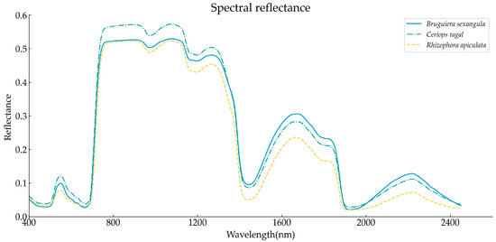
Figure 1.
Average spectral curves of three mangrove species.
In addition, the reflectance of C. tagal was significantly higher than that of B. sexangula and R. apiculata in the visible band and in the 800–1300 nm interval, whereas in the 1500–1800 nm and 2100–2300 nm intervals, the reflectance of B. sexangula was higher and the reflectance of R. apiculata in each band was relatively smaller than that of the other two mangrove species.
3.3. Successive Projection Algorithm for Filtering Feature Bands
The continuous projection method can maximize the screening of the characteristic wavelengths that contain the key information of the spectral reflection curve, and the covariance between variables is small. Application of the method achieves dimensionality reduction of the hyperspectral data, effectively reduces the input variables in the model operation, and improves the efficiency of the model operation. The results of the feature bands screened using the continuous projection algorithm are shown in Figure 2 and Table 2. For both the OR and FD data, the feature bands screened by the SPA were more distributed in the parts with evident changes in characteristics, such as wave peaks or troughs, which reduced the model input variables while retaining the feature information of the spectrum as much as possible.
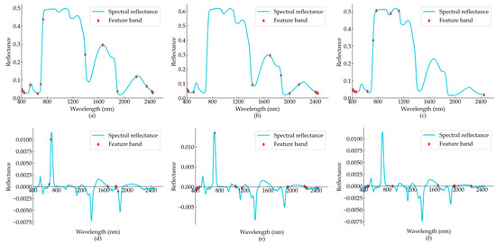
Figure 2.
Results of SPA feature band screening. (a–c) Screening results of the origin spectral data of B. sexangula, C. tagal, and R. apiculata, respectively; (d–f) screening results of the first-order differential spectral data of B. sexangula, C. tagal, and R. apiculata, respectively.
Table 2.
Feature band statistics.
We extracted more than ten feature bands from the different spectral treatments of each mangrove species using SPA. Except for the first-order differential transformation spectra of B. sexangula, six feature bands were extracted. Finally, we combined the original spectra and first-order differentially transformed spectra as the feature set for this species, with 22 feature bands extracted for B. sexangula, 30 for C. tagal, and 25 for R. apiculata.
3.4. Model Building
Based on the feature bands screened by SPA and the measured SPAD values, XGBoost, RF, PLS, and AdaBoost regression models were developed for the 42 training samples from the three mangrove species.
3.4.1. SPAD Regression Model of B. sexangula
The eight regression models built using the original spectral data and the first-order differential spectral data of B. sexangula are shown in Figure 3. For the OR data, the AdaBoost model had the highest modeling accuracy, with an R2 of 0.98 and the smallest RMSE of 0.79. For the FD data, both the XGBoost and AdaBoost models had high accuracy, with an R2 of 0.99; however, the RMSE of the XGBoost model was smaller at 0.61. For both the OR and FD data, the accuracy of the PLS regression model was significantly lower than that of the other three models.
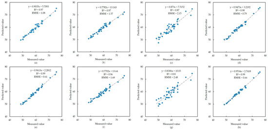
Figure 3.
Modeling results of B. sexangula. (a–d) Scatter plots of XGBoost, RF, PLS and AdaBoost models built using the original spectral data, respectively; (e–h) scatter plots of XGBoost, RF, PLS and AdaBoost models built using the first-order differential spectral data, respectively.
3.4.2. SPAD Regression Model of C. tagal
The modeling results based on the spectral data and SPAD values of C. tagal are shown in Figure 4. As with the modeling results of B. sexangula, the modeling accuracy of the PLS model for both spectral data was also the lowest, and the distribution of its data points was more discrete, especially for the modeling of the original spectral data; the R2 was only 0.71 and the RMSE was 2.60, which was significantly higher than that of the other models. In addition, the four regression models based on FD data have slightly improved accuracy compared with the regression models based on FD data, as shown by the different degrees of improvement in R2 and reduction in RMSE; the best accuracy is the AdaBoost model based on FD data, with an R2 of 0.99 and an RMSE of 0.49.
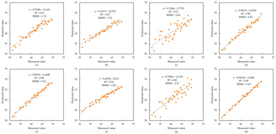
Figure 4.
Modeling results of C. tagal. (a–d) Scatter plots of XGBoost, RF, PLS and AdaBoost models built using the original spectral data, respectively; (e–h) scatter plots of XGBoost, RF, PLS and AdaBoost models built using the first-order differential spectral data, respectively.
3.4.3. SPAD Regression Model of R. apiculata
The modeling results of R. apiculata are presented in Figure 5, showing that the PLS model, based on OR data, had the worst accuracy of all regression models built for the three mangrove plants, with an R2 of only 0.64 and an RMSE of 2.68. However, the accuracy of the AdaBoost model based on the FD data is very high, with R2 reaching 0.99 and only 0.11 for the RMSE value. The data points are densely distributed on a 1:1 diagonal, with only a few sample points deviating from the 1:1 diagonal. In terms of the overall modeling accuracy, AdaBoost > XGBoost > RF > PLS, and it is evident that a first-order differential transformation of the OR data can improve the modeling accuracy.
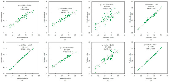
Figure 5.
Modeling results of R. apiculata. (a–d) Scatter plots of XGBoost, RF, PLS and AdaBoost models built using the original spectral data, respectively; (e–h) scatter plots of XGBoost, RF, PLS and AdaBoost models built using the first-order differential spectral data, respectively.
3.5. Evaluation of Model Validation Accuracy
We validated the accuracy of several regression models using the remaining 18 validation samples for each mangrove plant using three metrics, R2, RMSE and MAE, to evaluate the stability and accuracy of different spectral treatments and different regression models for predicting the SPAD values of mangrove plant leaves. The results are presented in Table 3 and Figure 6.
Table 3.
Validation of regression model accuracy.
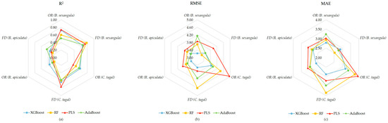
Figure 6.
Radar plot for model validation. (a) Radar plot of R2, (b) radar plot of RMSE, (c) radar plot of MAE.
Among the SPAD prediction models for B. sexangula, the validation accuracy of the RF model based on the FD data was the highest (R2 = 0.78, RMSE = 3.27, MAE = 2.52), whereas the AdaBoost model exhibited extremely high modeling accuracy, and its validation accuracy was the worst among the four models. For C. tagal, the best validation accuracy was for the PLS model based on the FD data (R2 = 0.77, RMSE = 3.70, MAE = 3.21), which was a significant improvement compared with the PLS model based on the OR data (R2 = 0.37, RMSE = 4.96, MAE = 3.95). The validation accuracy of the prediction models of R. apiculata is poor, and the accuracy decreases significantly compared with that of the modeling, and its R2 is mostly distributed in the interval of 0.2–0.4. Only the validation accuracy of the AdaBoost model based on the FD data is a little better, but its R2 is only 0.44, and the RMSE and MAE are 3.38 and 2.81, respectively.
4. Discussion
The chlorophyll content of leaves is an important indicator of plant growth and development, and many researchers have conducted related studies on remote sensing estimation of chlorophyll content in leaves [40,41,42]. However, relatively few studies have been conducted on the rapid prediction of chlorophyll content in the leaves of multiple mangrove species. The rapid prediction of leaf chlorophyll content in a variety of mangrove plants based on hyperspectral techniques is beneficial for the accurate monitoring of the management and growth status of mangrove plants on a large scale and can also provide a basis for species classification studies based on differences in chlorophyll content. This study compared the accuracy and stability of four regression models (XGBoost, RF, PLS, and AdaBoost) in SPAD inversion based on hyperspectral data measured by an ASD geospectrometer, which can provide a methodological reference for leaf-scale SPAD prediction.
The volume of the hyperspectral data was large, and the correlation between the bands was strong. Before using hyperspectral data for data analysis, extraction of feature bands using feature selection methods and the elimination of bands that are not correlated with chlorophyll markedly reduces the complexity of the model and is an important part of realizing a reduced and simplified model for hyperspectral data [43,44]. Using SPA, we reduced the number of bands from 2051 to approximately 10–20 for both the OR and FD spectral data, which greatly reduced the dimensionality of the data. However, when the feature bands were extracted, sometimes the number of bands given by SPA was not the number of bands corresponding to the smallest RMSE; therefore, we assumed that the optimal number of feature bands should be shuffled by combining the effects of the number of bands and the RMSE value on the model. In addition, the feature bands of both the OR and FD data were mainly concentrated in the parts of the wave peaks and troughs with more evident changes in reflectance (Figure 2), indicating that the feature bands extracted by the SPA retained well the characteristic information of the spectra. The feature bands of the leaf spectra of the three mangrove species were extracted using the SPA.
We used four regression models to explore the inversion of SPAD. The RF and PLS models have been widely used for the prediction of the elemental content of vegetation, confirming the universality of these two models, whereas the XGBoost and AdaBoost models are still relatively rarely used for the prediction of plant physiological and biochemical indicators. The RF model employs a modified CART decision tree as a learner, which significantly enhances its ability to handle nonlinear multiple-compound regression problems. As a decision tree is split and combined based on a tree structure, it can adapt to variable nonlinear data distributions, facilitating the handling of various complex data structures and improving the efficiency and accuracy of the algorithm [45,46]. PLS models have the advantage of removing multicollinearity and handling high-dimensional data, which can simplify the model and improve regression accuracy by compressing the dimensionality of independent variables [47]. AdaBoost is an integrated learning method that can be used to improve the accuracy of a classifier gradually by continuously iterating to adjust the weights of the samples. It uses multiple weak classifiers combined with a single strong classifier to achieve higher accuracy than a single weak classifier [48]. XGBoost is an integrated learning algorithm based on a tree model that is optimized and improved using a Gradient Boosting Machine algorithm. It is widely used in practical machine learning applications owing to its advantages of high accuracy and robustness, its capacity for handling missing values and high-dimensional features, it prevents overfitting, and is highly interpretable [49,50].
In this study, the PLS model was worse than the other four models, which may be related to the small number of samples in the training dataset, whereas an excessively small amount of data may lead to the inability of PLS to find effective patterns to complete the modeling, thus leading to poor modeling accuracy. In the validation of the models, the validation accuracy of all models decreased significantly compared to the modeling accuracy, which may be due to the use of the default parameters of the models and the relatively small number of validation samples, resulting in underfitting or overfitting of the models. Further in-depth research is needed to optimize the parameters of each regression model for the SPAD inversion of mangrove leaves. In addition, as shown in Table 3, regardless of the regression model, the validation accuracy showed a trend of B. sexangula > C. tagal > R. apiculate, with large differences between the species. The factors that lead to the large variation in the accuracy of the model between species are not yet known, which again requires in depth studies to explore the intrinsic reasons.
Previous studies have laid the foundation for studying chlorophyll inversion in mangrove plants. Table 4 shows some of the results of researchers who have achieved good inversion results by focusing more on narrow-band vegetation indices to improve the accuracy of inversion. We used several regression models to invert chlorophyll content and found that XGBoost was relatively stable. It was also interesting to observe the effects of combining the vegetation index with the XGBoost regression model. Additionally, many researchers are studying the use of stacking models for the inversion of metrics, which can combine the advantages of multiple algorithms and be more generalizable [51]. For example, Liu et al., (2023) constructed a high-precision stacked inversion model for apple leaf chlorophyll content based on boosting and stacking strategies; the R2 value of its validation set reached 0.9644, which was better than that of the traditional integrated learning model [52]. Lin et al., (2022) constructed a stacked AdaBoost model to invert the heavy metal content in soil; the stacked model was more stable and had better prediction accuracy than the traditional single machine learning model [53]. The performance of the stacking model during the inversion of leaf SPAD in mangrove plants will be the focus of future research.
Table 4.
Comparison of other research results with this paper.
The aim of this study was to investigate the accuracy and stability of SPAD inversion of mangrove plant leaves using hyperspectral data to provide theoretical support for the monitoring of mangrove growth. In addition, the research in this study was mainly based on inversion studies conducted using machine learning models. Deep learning models can effectively deal with nonlinear relationships, do not require manual extraction of features, and can learn the best feature representation adaptively, thus improving the generalization ability of the model and having higher prediction advantages [57]. They are now also gradually being applied to the inversion studies of some plant physiological and biochemical indicators [58,59]. Furthermore, the UAV technology is becoming more mature and is a better choice for remote sensing data acquisition. Compared to other remote sensing platforms, UAVs have high temporal and spatial resolution imaging capabilities, which are cost-effective and highly adaptable [60]. Many researchers have confirmed that combining UAV hyperspectral data with LiDAR data can effectively improve inversion accuracy [61,62], which will also be a new trend in studying SPAD inversion.
5. Conclusions
In this study, we used SPA to screen hyperspectral data for feature bands, built and validated four regression models based on the feature bands, and determined the SPAD values. The following conclusions were drawn.
- The leaves of B. sexangula had lower SPAD measurements than those of C. tagal and R. apiculata, and plants with higher leaf SPAD measurements had less variation in SPAD measurements.
- The accuracy and stability of the model established using first-order differentially transformed spectral data were slightly higher than those established using the original spectral data. First-order differential transformation of the original spectral data can improve the model accuracy.
- The PLS model was found to be the most suitable model for the SPAD inversion of B. sexangula leaves, whereas the most suitable model for SPAD inversion of C. tagal and R. apiculata leaves was found to be the XGBoost model.
- The XGBoost model had better adaptability to the leaf SPAD inversion of different species, and its stability is the best.
Author Contributions
Conceptualization, H.L. and W.L.; methodology, L.C. and J.W. (Junjie Wang); data curation, Z.D. and W.L.; funding acquisition, W.L.; project administration, Y.L. and J.W. (Jinzhi Wang); resources, W.L.; software, X.Z. (Xiajie Zhai) and X.Z. (Xinsheng Zhao); investigation, W.L., Z.D. and L.C.; visualization, J.L. and W.L.; writing—original draft, H.L.; writing—review and editing, L.C., Y.L., J.W. (Jinzhi Wang), J.W. (Junjie Wang) and W.L. All authors have read and agreed to the published version of the manuscript.
Funding
This research was funded by The Special Fund of Chinese Central Government for Basic Scientific Research Operations in Commonweal Research Institutes (CAFYBB2021MC006).
Data Availability Statement
All data included in this study are available upon request by contact with the corresponding author.
Conflicts of Interest
The authors declare no conflict of interest.
References
- Jia, P.H.; Huang, W.D.; Zhang, Z.Y.; Cheng, J.X.; Xiao, Y.L. The carbon sink of mangrove ecological restoration between 1988–2020 in Qinglan Bay, Hainan Island, China. Forests 2022, 13, 1547. [Google Scholar] [CrossRef]
- Dali, G.L.A.; Aheto, D.W.; Blay, J. Mangrove resource utilization and impacts in the Pra and Kakum estuaries of Ghana. Reg. Stud. Mar. Sci. 2023, 63, 103035. [Google Scholar] [CrossRef]
- Murdiyarso, D.; Purbopuspito, J.; Kauffman, J.B.; Warren, M.W.; Sasmito, S.D.; Donato, D.C.; Manuri, S.; Krisnawati, H.; Taberima, S.; Kurnianto, S. The potential of indonesian mangrove forests for global climate change mitigation. Nat. Clim. Chang. 2015, 5, 1089–1092. [Google Scholar] [CrossRef]
- Pennings, S.C.; Glazner, R.M.; Hughes, Z.J.; Kominoski, J.S.; Armitage, A.R. Effects of mangrove cover on coastal erosion during a hurricane in Texas, USA. Ecology 2021, 102, e03309. [Google Scholar] [CrossRef]
- Cinco-Castro, S.; Herrera-Silveira, J. Vulnerability of mangrove ecosystems to climate change effects: The case of the Yucatan Peninsula. Ocean. Coast. Manag. 2020, 192, 105196. [Google Scholar] [CrossRef]
- Thomas, N.; Lucas, R.; Bunting, P.; Hardy, A.; Rosenqvist, A.; Simard, M. Distribution and drivers of global mangrove forest change, 1996–2010. PLoS ONE 2017, 12, e0179302. [Google Scholar] [CrossRef]
- Feng, Z.Y.; Tan, G.M.; Xia, J.Q.; Shu, C.W.; Chen, P.; Wu, M.W.; Wu, X.M. Dynamics of mangrove forests in Shenzhen Bay in response to natural and anthropogenic factors from 1988 to 2017. J. Hydrol. 2020, 591, 125271. [Google Scholar] [CrossRef]
- Baloloy, A.B.; Blanco, A.C.; Ana, R.R.C.S.; Nadaoka, K. Development and application of a new mangrove vegetation index (MVI) for rapid and accurate mangrove mapping. ISPRS J. Photogramm. Remote Sens. 2020, 166, 95–117. [Google Scholar] [CrossRef]
- Li, W.; Cui, L.J.; Zhang, M.Y.; Wang, Y.F.; Zhang, Y.Q.; Lei, Y.R.; Zhao, X.S. Effect of mangrove restoration on crab burrow density in Luoyangjiang Estuary, China. For. Ecosyst. 2015, 2, 21. [Google Scholar] [CrossRef]
- Rodríguez-Rodríguez, J.A.; Mancera-Pineda, J.E.; Tavera, H. Mangrove restoration in Colombia: Trends and lessons learned. For. Ecol. Manag. 2021, 496, 119414. [Google Scholar] [CrossRef]
- Croft, H.; Chen, J.M.; Luo, X.; Bartlett, P.; Chen, B.; Staebler, R.M. Leaf chlorophyll content as a proxy for leaf photosynthetic capacity. Glob. Chang. Biol. 2017, 23, 3513–3524. [Google Scholar] [CrossRef] [PubMed]
- Amirruddin, A.D.; Muharam, F.M.; Ismail, M.H.; Ismail, M.F.; Tan, N.P.; Karam, D.S. Hyperspectral remote sensing for assessment of chlorophyll sufficiency levels in mature oil palm (Elaeis guineensis) based on frond numbers: Analysis of decision tree and random forest. Comput. Electron. Agric. 2020, 169, 105221. [Google Scholar]
- Wu, Q.; Zhang, Y.P.; Zhao, Z.W.; Xie, M.; Hou, D.Y. Estimation of relative chlorophyll content in spring wheat based on multi-temporal UAV remote sensing. Agronomy 2023, 13, 211. [Google Scholar] [CrossRef]
- Wang, Y.W.; Tan, S.Y.; Jia, X.N.; Qi, L.; Liu, S.S.; Lu, H.H.; Wang, C.G.; Liu, W.W.; Zhao, X.; He, L.X.; et al. Estimating relative chlorophyll content in rice leaves using unmanned aerial vehicle multi-spectral images and spectral–textural analysis. Agronomy 2023, 13, 1541. [Google Scholar] [CrossRef]
- Brown, L.A.; Williams, O.; Dash, J. Calibration and characterisation of four chlorophyll meters and transmittance spectroscopy for non-destructive estimation of forest leaf chlorophyll concentration. Agric. For. Meteorol. 2022, 323, 109059. [Google Scholar] [CrossRef]
- Connelly, X.M. The Use of a chlorophyll meter (SPAD-502) for field determinations of red mangrove (Rhizophora mangle L.) leaf chlorophyll amount. NASA Univ. Res. Cent. Technol. Adv. Educ. Aeronaut. Space Auton. Earth Environ. 1997, 1, 187–190. [Google Scholar]
- Neres, J.; Dodonov, P.; Mielke, M.S.; Strenzel, G.M.R. Relationships between portable chlorophyll meter estimates for the red mangrove tree (Rhizophora mangle L.). Ocean. Coast. Res. 2020, 68, e20308. [Google Scholar] [CrossRef]
- Liu, W.W.; Li, M.J.; Zhang, M.Y.; Wang, D.A.; Guo, Z.L.; Long, S.Y.; Yang, S.; Wang, H.N.; Li, W.; Hu, Y.K.; et al. Estimating leaf mercury content in Phragmites australis based on leaf hyperspectral reflectance. Ecosyst. Health Sustain. 2020, 6, 1726211. [Google Scholar] [CrossRef]
- Tang, X.Y.; Dou, Z.G.; Cui, L.J.; Liu, Z.J.; Gao, C.J.; Wang, J.J.; Li, J.; Lei, Y.R.; Zhao, X.S.; Zhai, X.J.; et al. Hyperspectral prediction of mangrove leaf stoichiometries in different restoration areas based on machine learning models. J. Appl. Remote Sens. 2022, 16, 034525. [Google Scholar] [CrossRef]
- Jiang, Y.F.; Zhang, L.; Yan, M.; Qi, J.G.; Fu, T.M.; Fan, S.X.; Chen, B.W. High-resolution mangrove forests classification with machine learning using worldview and UAV hyperspectral data. Remote Sens. 2021, 13, 1529. [Google Scholar] [CrossRef]
- Zhao, C.P.; Qin, C.Z. Identifying large-area mangrove distribution based on remote sensing: A binary classification approach considering subclasses of non-mangroves. Int. J. Appl. Earth Obs. Geoinf. 2022, 108, 102750. [Google Scholar]
- Yang, G.; Huang, K.; Sun, W.W.; Meng, X.C.; Mao, D.H.; Ge, Y. Enhanced mangrove vegetation index based on hyperspectral images for mapping mangrove. ISPRS J. Photogramm. Remote Sens. 2022, 189, 236–254. [Google Scholar] [CrossRef]
- Pandey, P.C.; Anand, A.; Srivastava, P.K. Spatial distribution of mangrove forest species and biomass assessment using field inventory and earth observation hyperspectral data. Biodivers. Conserv. 2019, 28, 2143–2162. [Google Scholar] [CrossRef]
- Dou, Z.G.; Cui, L.J.; Li, J.; Zhu, Y.N.; Gao, C.J.; Pan, X.; Lei, Y.R.; Zhang, M.Y.; Zhao, X.S.; Li, W. Hyperspectral estimation of the chlorophyll content in short-term and long-term restorations of mangrove in Quanzhou Bay estuary, China. Sustainability 2018, 10, 1127. [Google Scholar] [CrossRef]
- Wang, J.J.; Xu, Y.; Wu, G.F. The integration of species information and soil properties for hyperspectral estimation of leaf biochemical parameters in mangrove forest. Ecol. Indic. 2020, 115, 106467. [Google Scholar] [CrossRef]
- Zhen, J.N.; Jiang, X.P.; Xu, Y.; Miao, J.; Zhao, D.M.; Wang, J.J.; Wang, J.Z.; Wu, G.F. Mapping leaf chlorophyll content of mangrove forests with sentinel-2 images of four periods. Int. J. Appl. Earth Obs. Geoinf. 2021, 102, 102387. [Google Scholar] [CrossRef]
- Jiang, X.P.; Zhen, J.N.; Miao, J.; Zhao, D.M.; Shen, Z.; Jiang, J.C.; Gao, C.J.; Wu, G.F.; Wang, J.J. Newly-developed three-band hyperspectral vegetation index for estimating leaf relative chlorophyll content of mangrove under different severities of pest and disease. Ecol. Indic. 2022, 140, 108978. [Google Scholar] [CrossRef]
- Fu, B.L.; Deng, L.C.; Zhang, L.; Qin, J.L.; Liu, M.; Jia, M.M.; He, H.C.; Deng, T.F.; Gao, E.T.; Fan, D.L. Estimation of mangrove canopy chlorophyll content using hyperspectral image and stacking ensemble regression algorithm. Natl. Remote Sens. Bull. 2022, 26, 1182–1205. [Google Scholar] [CrossRef]
- Chen, X.H.; Chen, Z.Z.; Lei, J.R.; Wu, T.T.; Li, Y.L. Distribution characteristics of active organic carbon components in sediments of typical community types of mangrove wetland in Qinglan Port. Acta Ecol. Sin. 2022, 42, 4572–4581. [Google Scholar]
- Zhen, J.N.; Liao, J.J.; Shen, G.Z. Remote sensing monitoring and analysis on the dynamics of mangrove forests in Qinglan Habor of Hainan province since 1987. Wetl. Sci. 2019, 17, 44–51. [Google Scholar]
- Croft, H.; Chen, J.M.; Zhang, Y. The applicability of empirical vegetation indices for determining leaf chlorophyll content over different leaf and canopy structures. Ecol. Complex. 2014, 17, 119–130. [Google Scholar] [CrossRef]
- Wu, J.D.; Wang, D.; Rosen, C.J.; Bauer, M.E. Comparison of petiole nitrate concentrations, SPAD chlorophyll readings, and QuickBird satellite imagery in detecting nitrogen status of potato canopies. Field Crops Res. 2007, 101, 96–103. [Google Scholar] [CrossRef]
- Xu, Y.; Wang, J.J.; Xia, A.Q.; Zhang, K.Y.; Dong, X.Y.; Wu, K.P.; Wu, G.F. Continuous wavelet analysis of leaf reflectance improves classification accuracy of mangrove species. Remote Sens. 2019, 11, 254. [Google Scholar] [CrossRef]
- Wang, J.J.; Cui, L.J.; Gao, W.X.; Shi, T.Z.; Chen, Y.Y.; Gao, Y. Prediction of low heavy metal concentrations in agricultural soils using visible and near-infrared reflectance spectroscopy. Geoderma 2014, 216, 1–9. [Google Scholar] [CrossRef]
- Yang, H.Y.; Du, J.M. Classification of desert steppe species based on unmanned aerial vehicle hyperspectral remote sensing and continuum removal vegetation indices. Optik 2021, 247, 167877. [Google Scholar] [CrossRef]
- Araújo, M.C.U.; Saldanha, T.C.B.; Galvão, R.K.H.; Yoneyama, T.; Chame, H.C.; Visani, V. The successive projections algorithm for variable selection in spectroscopic multicomponent analysis. Chemom. Intell. Lab. Syst. 2001, 57, 65–73. [Google Scholar] [CrossRef]
- Lu, J.Q.; Qiu, H.B.; Zhang, Q.; Lan, Y.B.; Wang, P.P.; Wu, Y.; Mo, J.W.; Chen, W.D.; Niu, H.Y.; Wu, Z.Y. Inversion of chlorophyll content under the stress of leaf mite for jujube based on model PSO-ELM method. Front. Plant Sci. 2022, 13, 1009630. [Google Scholar] [CrossRef]
- Cui, L.J.; Dou, Z.G.; Liu, Z.J.; Zuo, X.Y.; Lei, Y.R.; Li, J.; Zhao, X.S.; Zhai, X.J.; Pan, X.; Li, W. Hyperspectral inversion of Phragmites communis carbon, nitrogen, and phosphorus stoichiometry using three models. Remote Sens. 2020, 12, 1998. [Google Scholar] [CrossRef]
- Liu, S.Y.; Zhang, B.; Yang, W.G.; Chen, T.T.; Zhang, H.; Lin, Y.D.; Tan, J.T.; Li, X.; Gao, Y.; Yao, S.Z.; et al. Quantification of physiological parameters of rice varieties based on multi-spectral remote sensing and machine learning models. Remote Sens. 2023, 15, 453. [Google Scholar] [CrossRef]
- Wang, S.Q.; Li, Y.; Ju, W.M.; Chen, B.; Chen, J.H.; Croft, H.; Mickler, R.A.; Yang, F.T. Estimation of leaf photosynthetic capacity from leaf chlorophyll content and leaf age in a subtropical evergreen coniferous plantation. J. Geophys. Res. Biogeosci. 2020, 125, e2019JG005020. [Google Scholar] [CrossRef]
- Shi, S.; Xu, L.; Gong, W.; Chen, B.W.; Chen, B.W.; Qu, F.F.; Tang, X.T.; Sun, J.; Yang, J. A convolution neural network for forest leaf chlorophyll and carotenoid estimation using hyperspectral reflectance. Int. J. Appl. Earth Obs. Geoinf. 2022, 108, 102719. [Google Scholar] [CrossRef]
- Xu, L.; Shi, S.; Gong, W.; Shi, Z.X.; Qu, F.F.; Tang, X.T.; Chen, B.W.; Sun, J. Improving leaf chlorophyll content estimation through constrained PROSAIL model from airborne hyperspectral and LiDAR data. Int. J. Appl. Earth Obs. Geoinf. 2022, 115, 103128. [Google Scholar] [CrossRef]
- Zhang, F.F.; Wu, S.W.; Liu, J.; Wang, C.K.; Guo, Z.Y.; Xu, A.A.; Pan, K.; Pan, X.Z. Predicting soil moisture content over partially vegetation covered surfaces from hyperspectral data with deep learning. Soil Sci. Soc. Am. J. 2021, 85, 989–1001. [Google Scholar] [CrossRef]
- Liu, J.B.; Xie, J.C.; Meng, T.T.; Dong, H. Organic matter estimation of surface soil using successive projection algorithm. Agron. J. 2021, 114, 1944–1951. [Google Scholar] [CrossRef]
- Ndlovu, H.S.; Odindi, J.; Sibanda, M.; Mutanga, O.; Clulow, A.; Chimonyo, V.G.P.; Mabhaudhi, T. A comparative estimation of maize leaf water content using machine learning techniques and unmanned aerial vehicle (UAV)-based proximal and remotely sensed data. Remote Sens. 2021, 13, 4091. [Google Scholar] [CrossRef]
- Wang, J.J.; Zhou, Q.; Shang, J.L.; Liu, C.; Zhuang, T.X.; Ding, J.J.; Xian, Y.Y.; Zhao, L.T.; Wang, W.L.; Zhou, G.S.; et al. UAV- and machine learning-based retrieval of wheat SPAD values at the overwintering stage for variety screening. Remote Sens. 2021, 13, 5166. [Google Scholar] [CrossRef]
- Rischbeck, P.; Elsayed, S.; Mistele, B.; Barmeier, G.; Heil, K.; Schmidhalter, U. Data fusion of spectral, thermal and canopy height parameters for improved yield prediction of drought stressed spring barley. Eur. J. Agron. 2016, 78, 44–59. [Google Scholar] [CrossRef]
- Ramzi, P.; Samadzadegan, F.; Reinartz, P. Classification of hyperspectral data using an AdaboostSVM technique applied on band clusters. IEEE J. Sel. Top. Appl. Earth Obs. Remote Sens. 2014, 7, 2066–2079. [Google Scholar] [CrossRef]
- Wei, L.F.; Wang, Z.; Huang, C.; Zhang, Y.; Wang, Z.X.; Xia, H.Q.; Cao, L.Q. Transparency estimation of narrow rivers by uav-borne hyperspectral remote sensing imagery. IEEE Access 2020, 8, 168137–168153. [Google Scholar] [CrossRef]
- Zhang, Y.; Xia, C.Z.; Zhang, X.Y.; Cheng, X.H.; Feng, G.Z.; Wang, Y.; Gao, Q. Estimating the maize biomass by crop height and narrowband vegetation indices derived from UAV-based hyperspectral images. Ecol. Indic. 2021, 129, 107985. [Google Scholar] [CrossRef]
- Tan, K.; Ma, W.B.; Chen, L.H.; Wang, H.M.; Du, Q.; Du, P.J.; Yan, B.K.; Liu, R.Y.; Li, H.D. Estimating the distribution trend of soil heavy metals in mining area from HYMAP airborne hyperspectral imagery based on ensemble learning. J. Hazard. Mater. 2021, 401, 123288. [Google Scholar] [CrossRef] [PubMed]
- Liu, Y.F.; Zhang, Y.; Jiang, D.Y.; Zhang, Z.Z.; Chang, Q.R. Quantitative assessment of apple mosaic disease severity based on hyperspectral images and chlorophyll content. Remote Sens. 2023, 15, 2202. [Google Scholar] [CrossRef]
- Lin, N.; Jiang, R.Z.; Li, G.J.; Yang, Q.; Li, D.L.; Yang, X.S. Estimating the heavy metal contents in farmland soil from hyperspectral images based on Stacked Adaboost ensemble learning. Ecol. Indic. 2022, 143, 109330. [Google Scholar] [CrossRef]
- Jiang, X.P.; Zhen, J.N.; Miao, J.; Zhao, D.M.; Wang, J.J.; Jia, S. Assessing mangrove leaf traits under different pest and disease severity with hyperspectral imaging spectroscopy. Ecol. Indic. 2021, 129, 107901. [Google Scholar] [CrossRef]
- George, R.; Padalia, H.; Sinha, S.K.; Kumar, A.S. Evaluating sensitivity of hyperspectral indices for estimating mangrove chlorophyll in middle Andaman Island, India. Environ. Monit. Assess. 2020, 191, 785. [Google Scholar] [CrossRef] [PubMed]
- Zhao, Y.X.; Yan, C.H.; Lu, S.; Wang, P.; Qiu, G.Y.; Li, R.L. Estimation of chlorophyll content in intertidal mangrove leaves with different thicknesses using hyperspectral data. Ecol. Indic. 2019, 106, 105511. [Google Scholar] [CrossRef]
- Zhang, Y.; Hui, J.; Qin, Q.M.; Sun, Y.H.; Zhang, T.Y.; Sun, H.; Li, M.Z. Transfer-learning-based approach for leaf chlorophyll content estimation of winter wheat from hyperspectral data. Remote Sens. Environ. 2021, 267, 112724. [Google Scholar] [CrossRef]
- Tian, Y.C.; Huang, H.; Zhou, G.Q.; Zhang, Q.; Tao, J.; Zhang, Y.L.; Lin, J.J. Aboveground mangrove biomass estimation in Beibu Gulf using machine learning and UAV remote sensing. Sci. Total Environ. 2021, 781, 146816. [Google Scholar] [CrossRef]
- Zhu, X.H.; Yang, Q.; Chen, X.Y.; Ding, Z.X. An approach for joint estimation of grassland leaf area index and leaf chlorophyll content from UAV hyperspectral data. Remote Sens. 2023, 15, 2525. [Google Scholar] [CrossRef]
- Sudu, B.; Rong, G.; Guga, S.; Li, K.; Zhi, F.; Guo, Y.; Zhang, J.; Bao, Y. Retrieving SPAD values of summer maize using UAV hyperspectral data based on multiple machine learning algorithm. Remote Sens. 2022, 14, 5407. [Google Scholar] [CrossRef]
- Dilmurat, K.; Sagan, V.; Moose, S. Ai-driven maize yield forecasting using unmanned aerial vehicle-based hyperspectral and LiDAR data fusion. ISPRS Ann. Photogramm. Remote Sens. Spat. Inf. Sci. 2022, V-3-2022, 193–199. [Google Scholar] [CrossRef]
- Tian, Y.; Huang, H.; Zhou, G.; Zhang, Q.; Xie, X.; Ou, J.; Zhang, Y.; Tao, J.; Lin, J. Mangrove biodiversity assessment using UAV LiDAR and hyperspectral data in China’s Pinglu canal estuary. Remote Sens. 2023, 15, 2622. [Google Scholar] [CrossRef]
Disclaimer/Publisher’s Note: The statements, opinions and data contained in all publications are solely those of the individual author(s) and contributor(s) and not of MDPI and/or the editor(s). MDPI and/or the editor(s) disclaim responsibility for any injury to people or property resulting from any ideas, methods, instructions or products referred to in the content. |
© 2023 by the authors. Licensee MDPI, Basel, Switzerland. This article is an open access article distributed under the terms and conditions of the Creative Commons Attribution (CC BY) license (https://creativecommons.org/licenses/by/4.0/).