
Assessment of Forest Road Models in Concession Areas in the Brazilian Amazon


 ,
,  , ,
, ,  and
and 
Abstract
1. Introduction
2. Materials and Methods
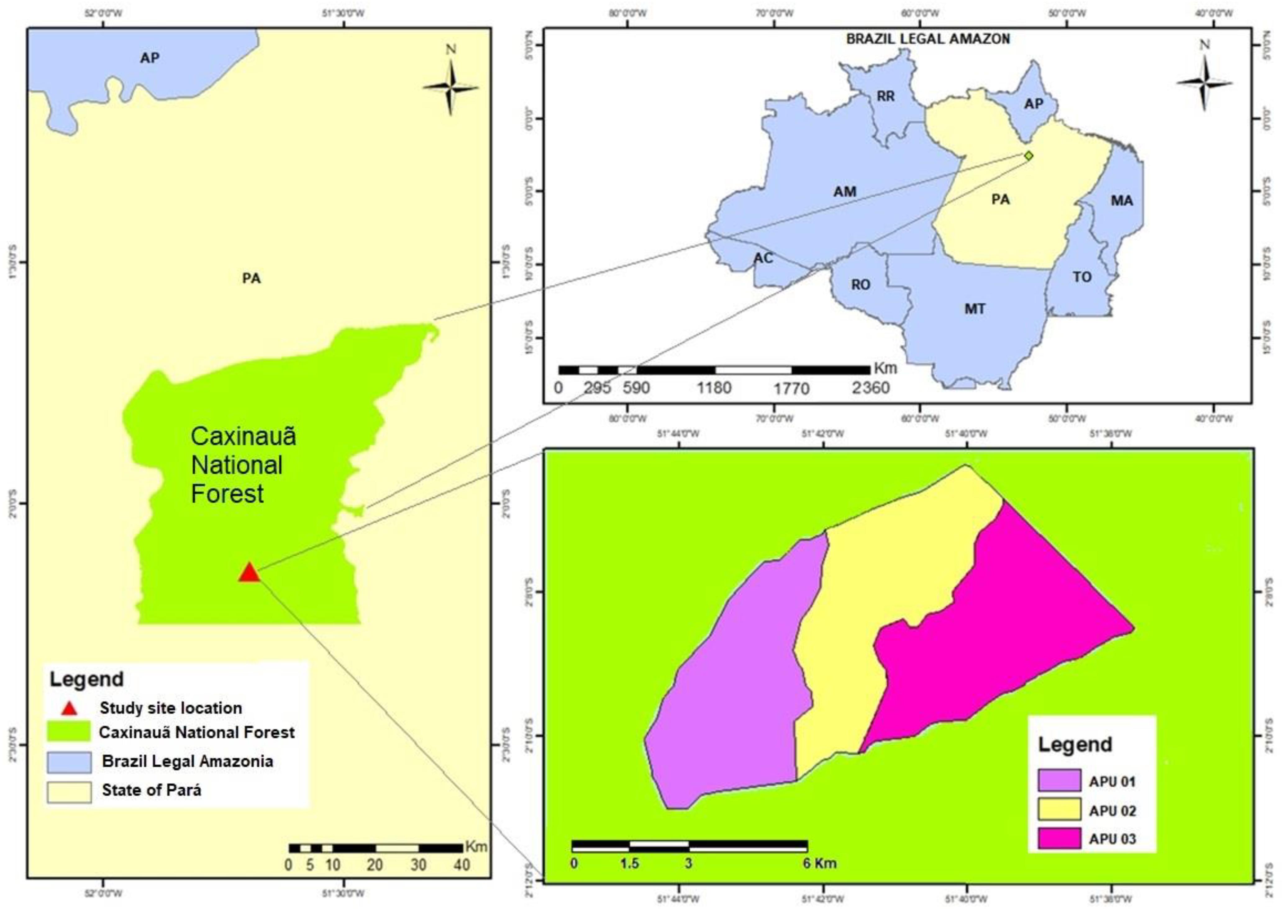
2.1. Study Site
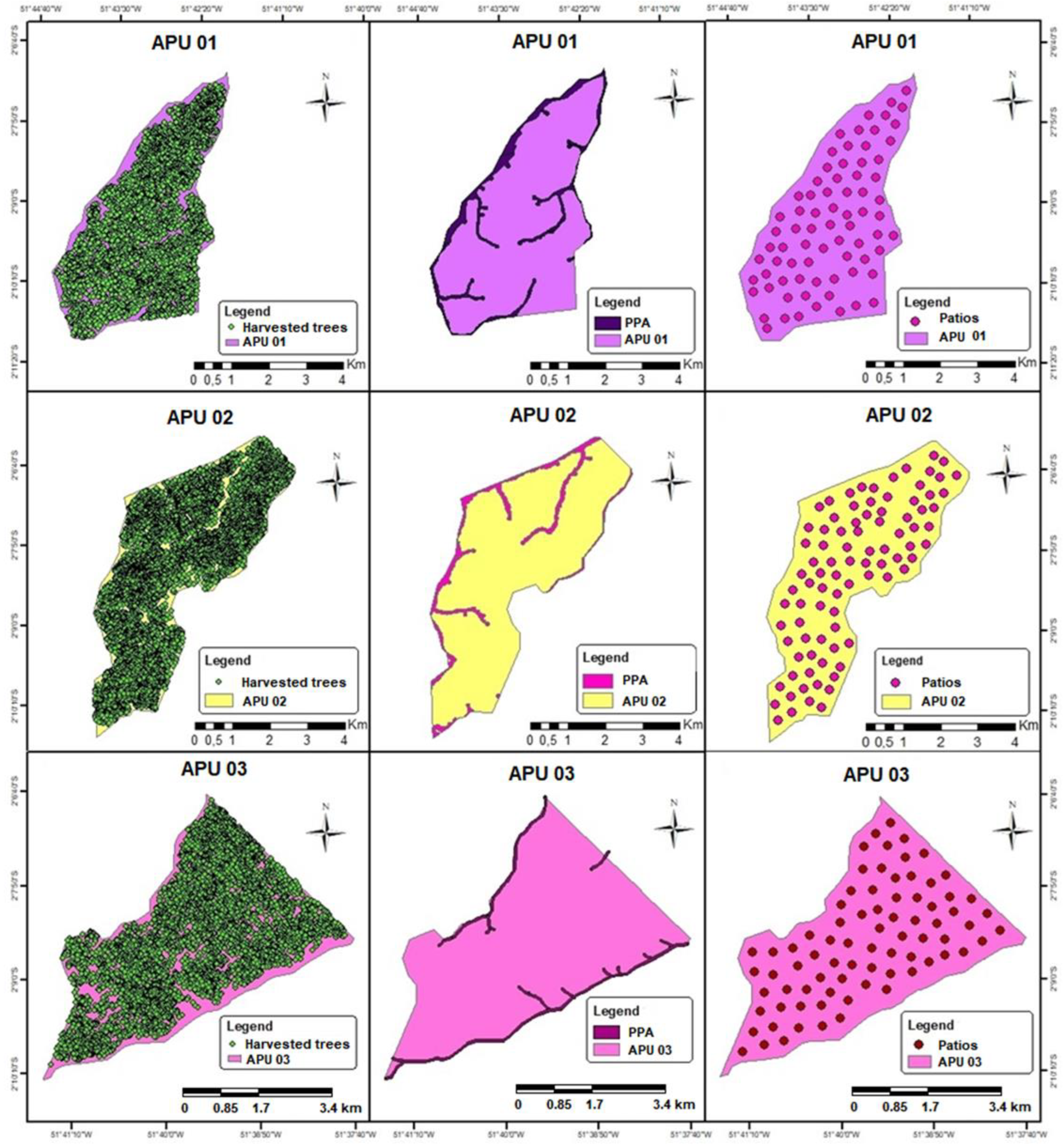
2.2. Field Datasets
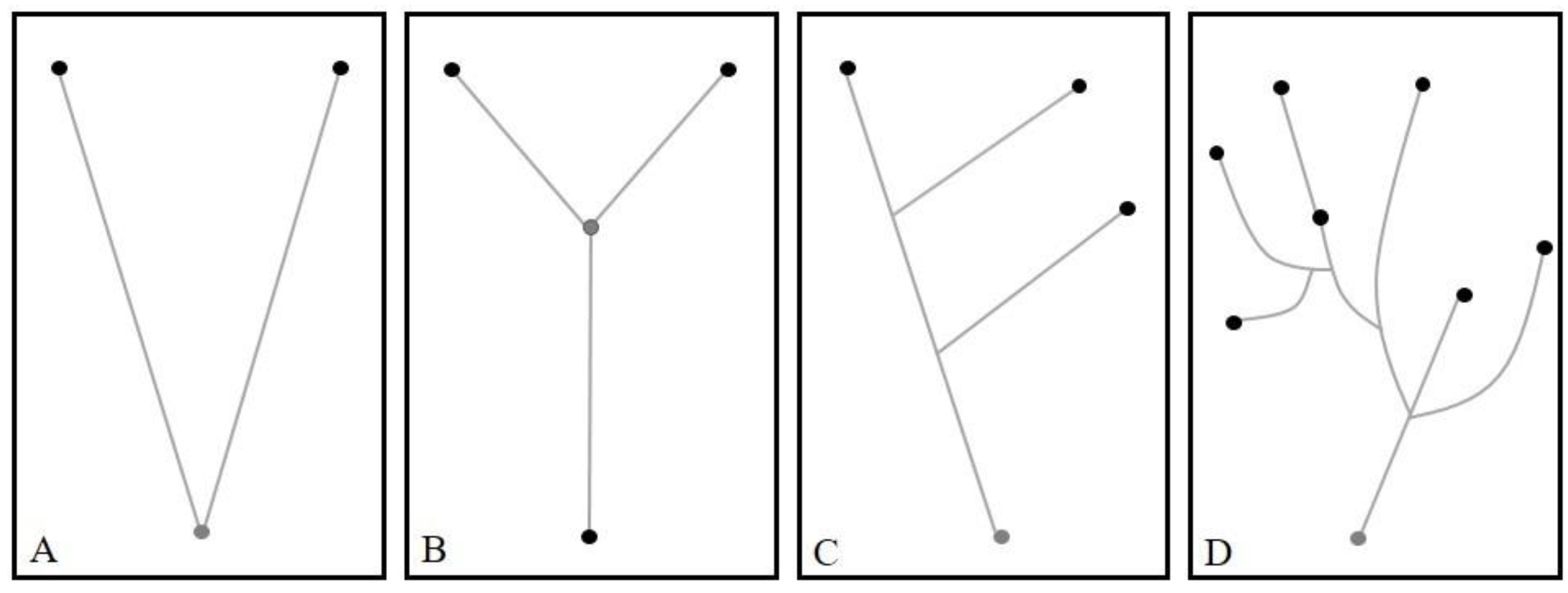
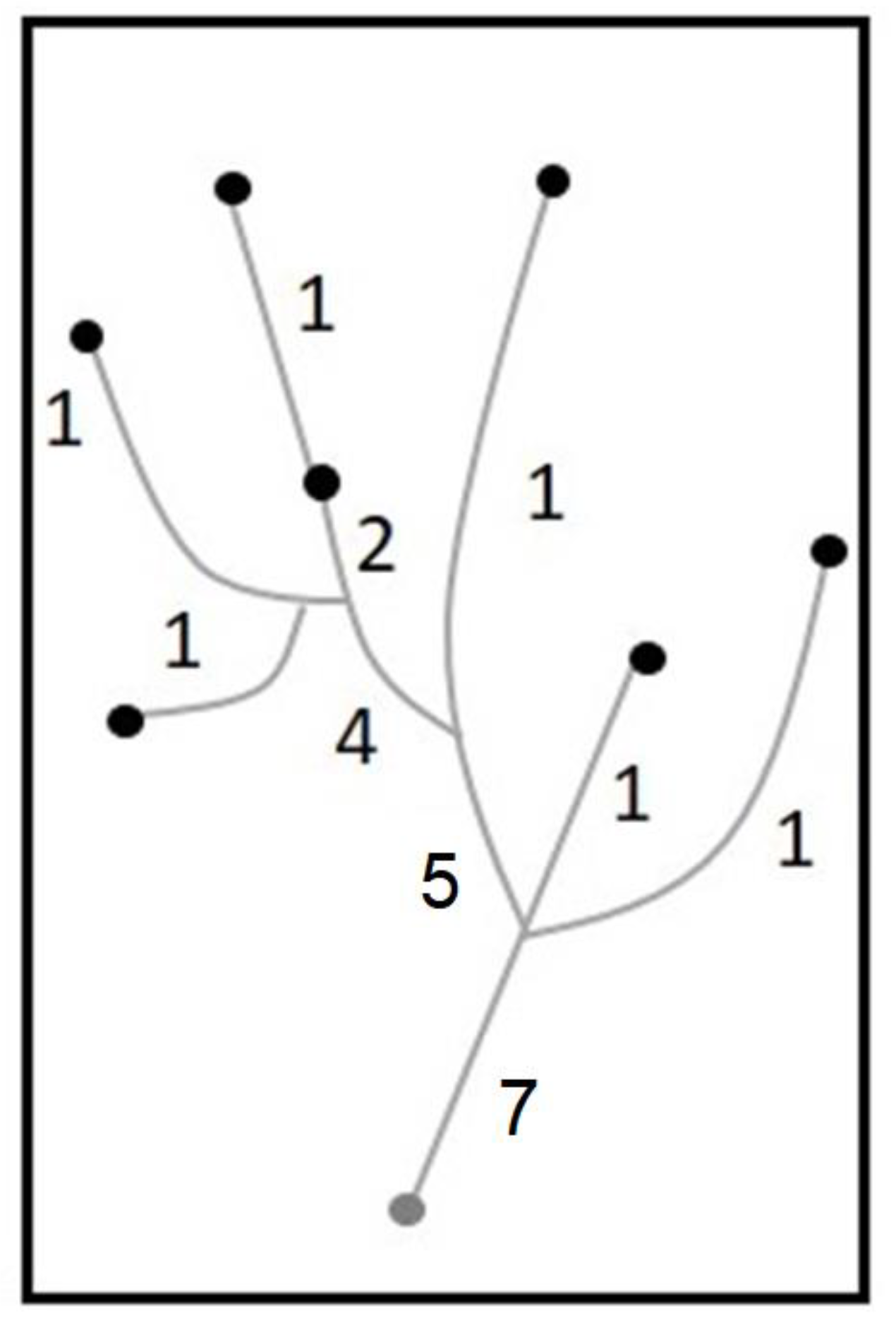
2.3. Forest Road Modeling
2.4. Modeling Assessment
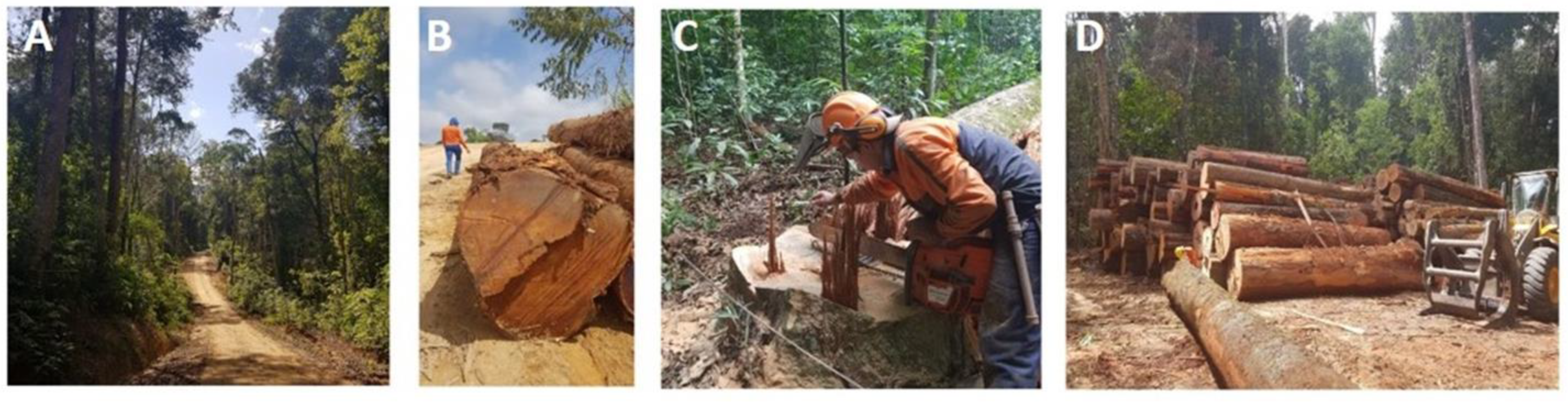
2.5. Assessment of Selective Logging Operations
2.5.1. Average Skid Distance (ASD)
2.5.2. Operational Costs
- (a)
- Depreciation:
- (b)
- Interests
- (c)
- Insurances
- (a)
- Fuel
- (b)
- Hydraulic oil
- (c)
- Motor oil
- (d)
- Maintenance and Repairs
- (e)
- Tires
- (f)
- Skidder Operator (SO)
- (g)
- Transportation Cost (TC)
- (h)
- Administration Cost (AC):
- (i)
- Total operational costs (TOC):
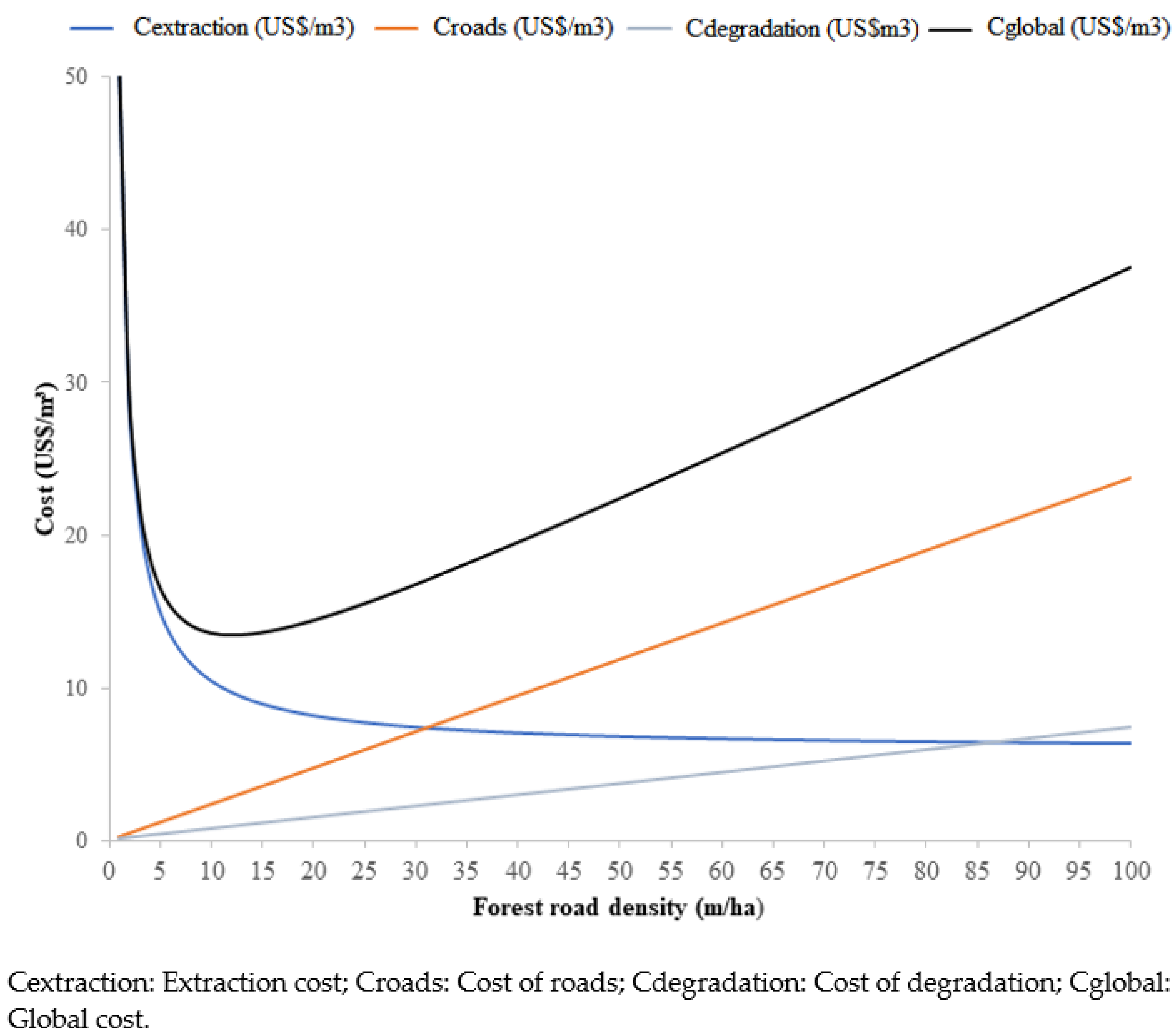
2.5.3. Optimum Road Density (ORD)
2.5.4. Acceptable Road Density
2.5.5. Optimum Separation of Secondary Roads
- (a)
- A total of 5 to 10 average skid distances (ASD) are assumed in which the skidder will potentially work (under the relief conditions), e.g., 100, 150, 200, 300, to 1000 m, and the log skidding cost is calculated on those road lengths.
- (b)
- By using a simplified formula 10,000/4*ASD, the corresponding optimum road densities (ORD, m/ha) are estimated for the log skidding distance. The ASD will increase as the ORD decreases.
- (c)
- The harvesting costs in relation to the log skidding distance (considering the type of equipment) and the corresponding cost of road construction, according to the road extent per hectare (considering the standard or category of the roads), were estimated. The harvesting costs increase as the log skidding distances increase, and the road construction costs decrease (for example, roads can be separated into two categories: permanent and temporary roads).
- (d)
- The corresponding costs (ASD + ORD) are added.
- (e)
- There will be some intermediate point between 100 m and 1000 m, where the sum will be the smallest one, which will be the optimum distance. Out of that distance there will be constructed too many or too few roads and log skidding at larger or shorter distances, normally resulting in higher costs of roads or harvesting. Because the theoretical ORD is equal to OSR/4, the distance among the selected roads will be equal to the selected ORD multiplied by 4.
2.5.6. Assessment of Skid Operations
3. Results
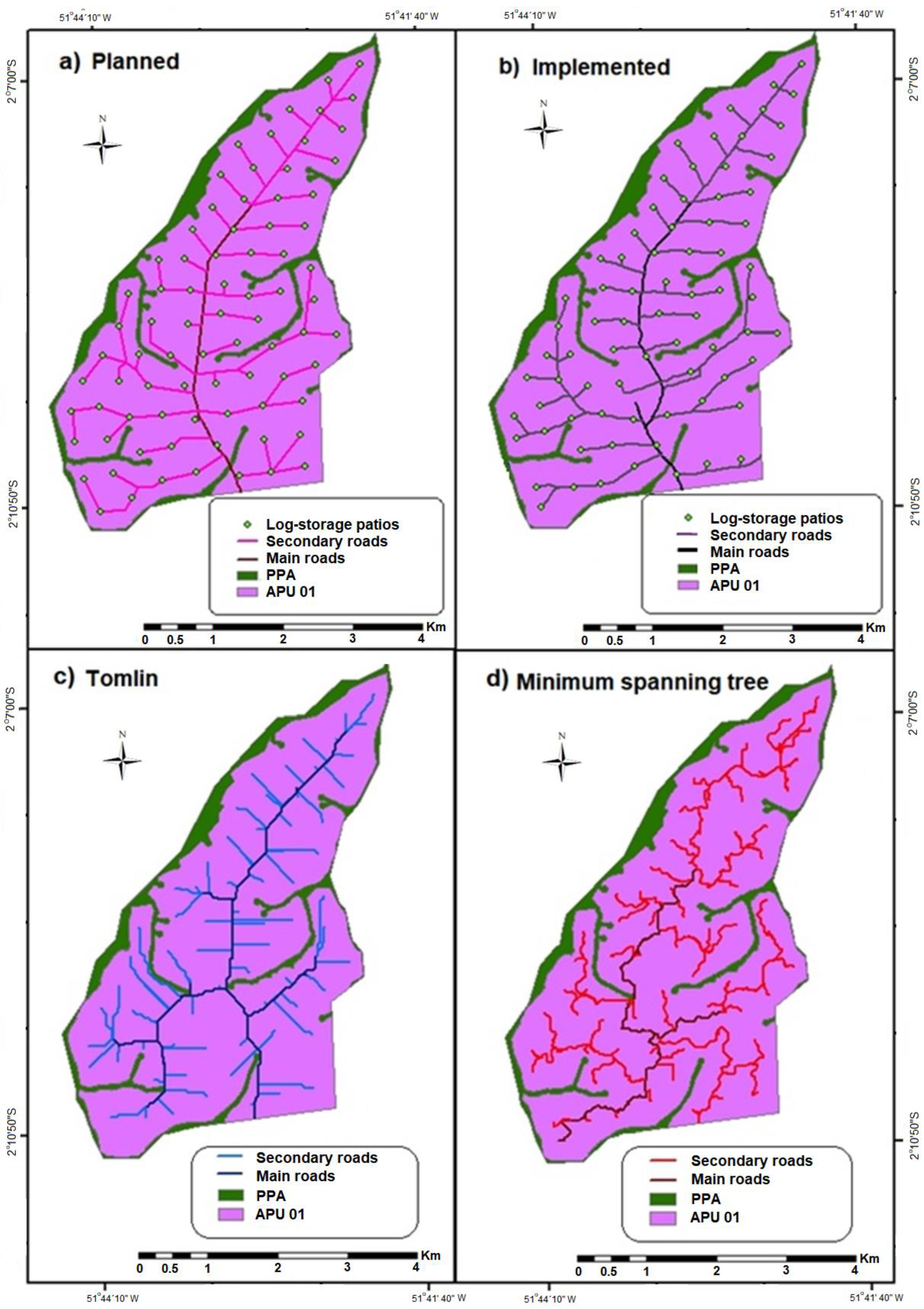
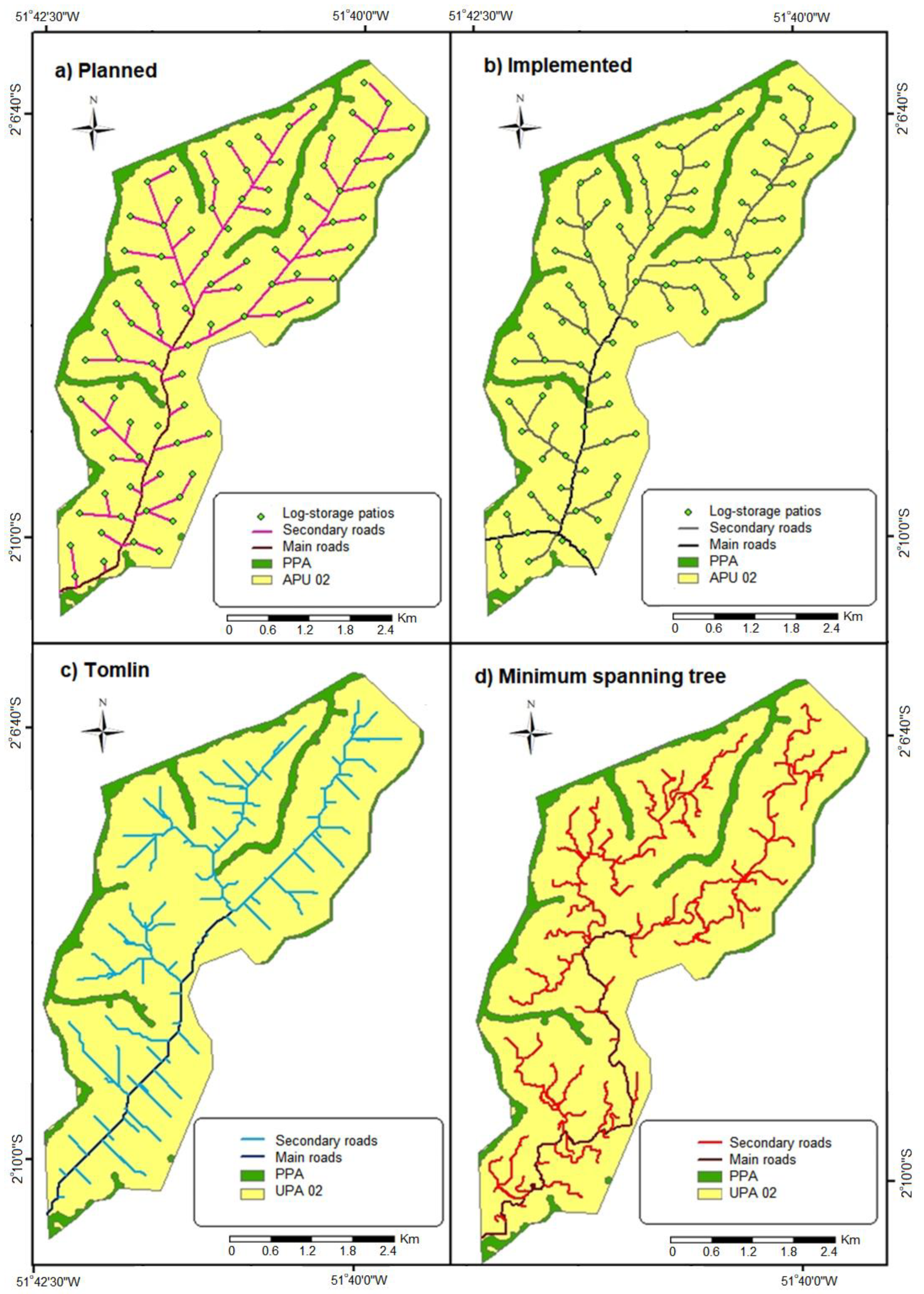
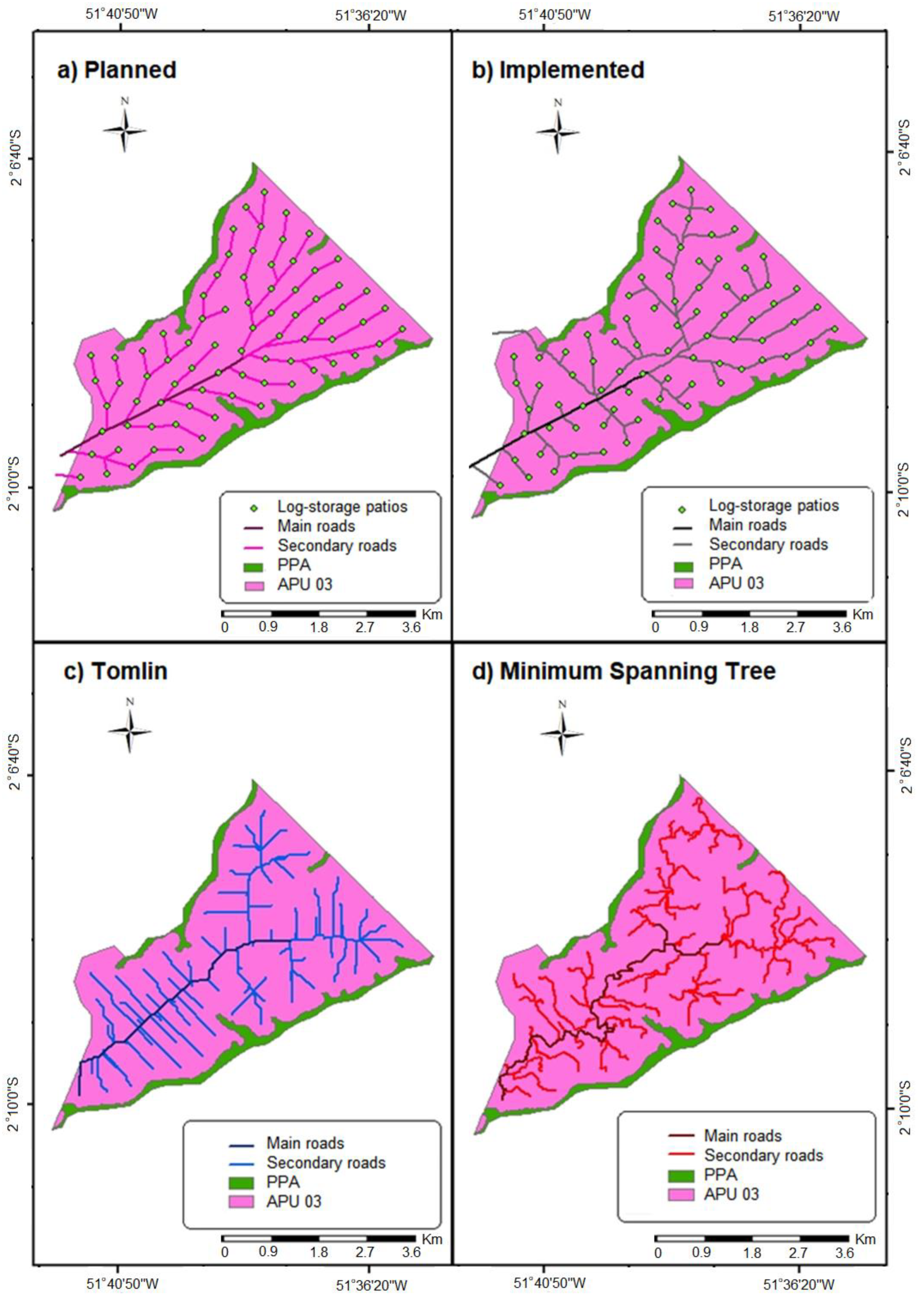
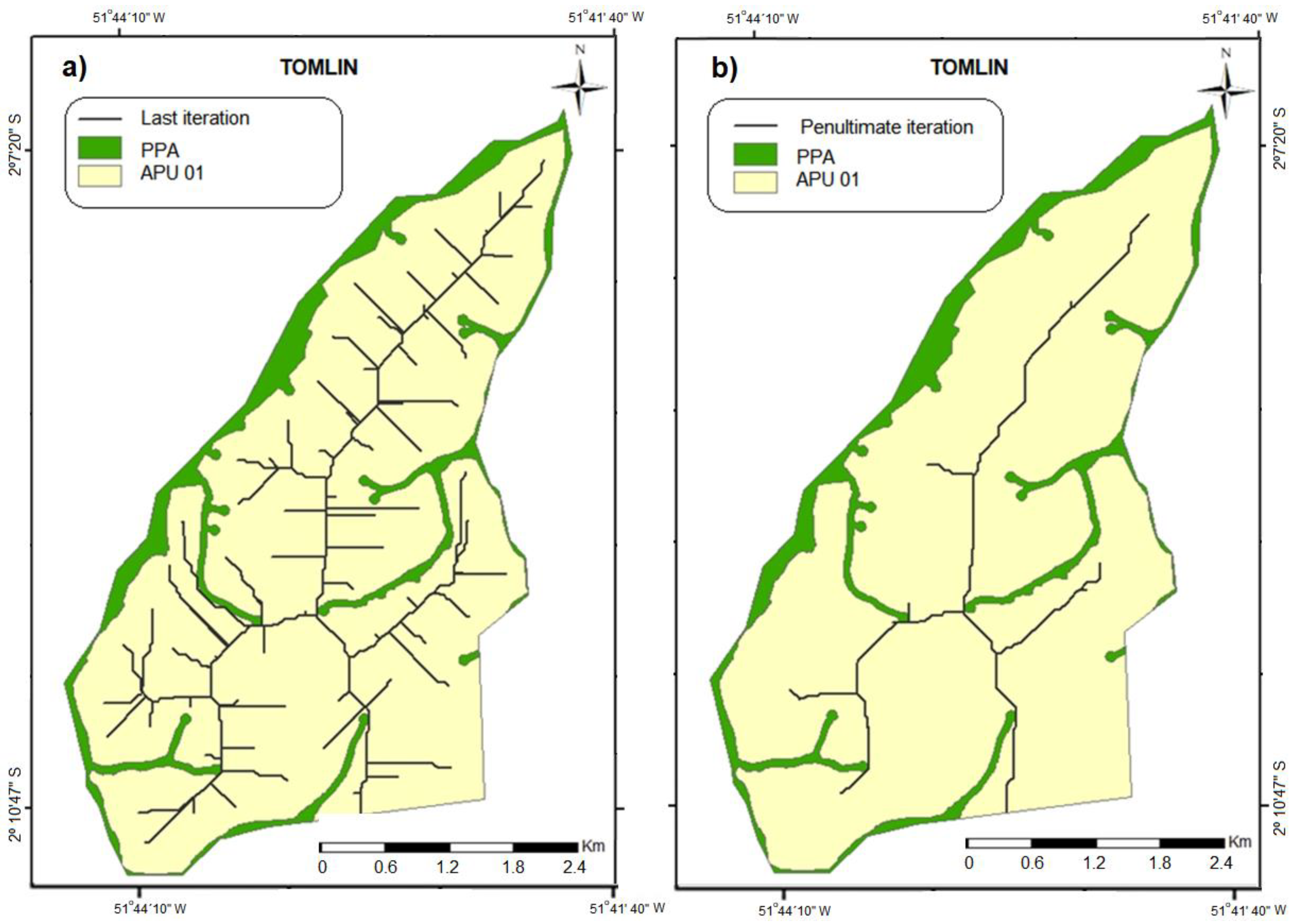
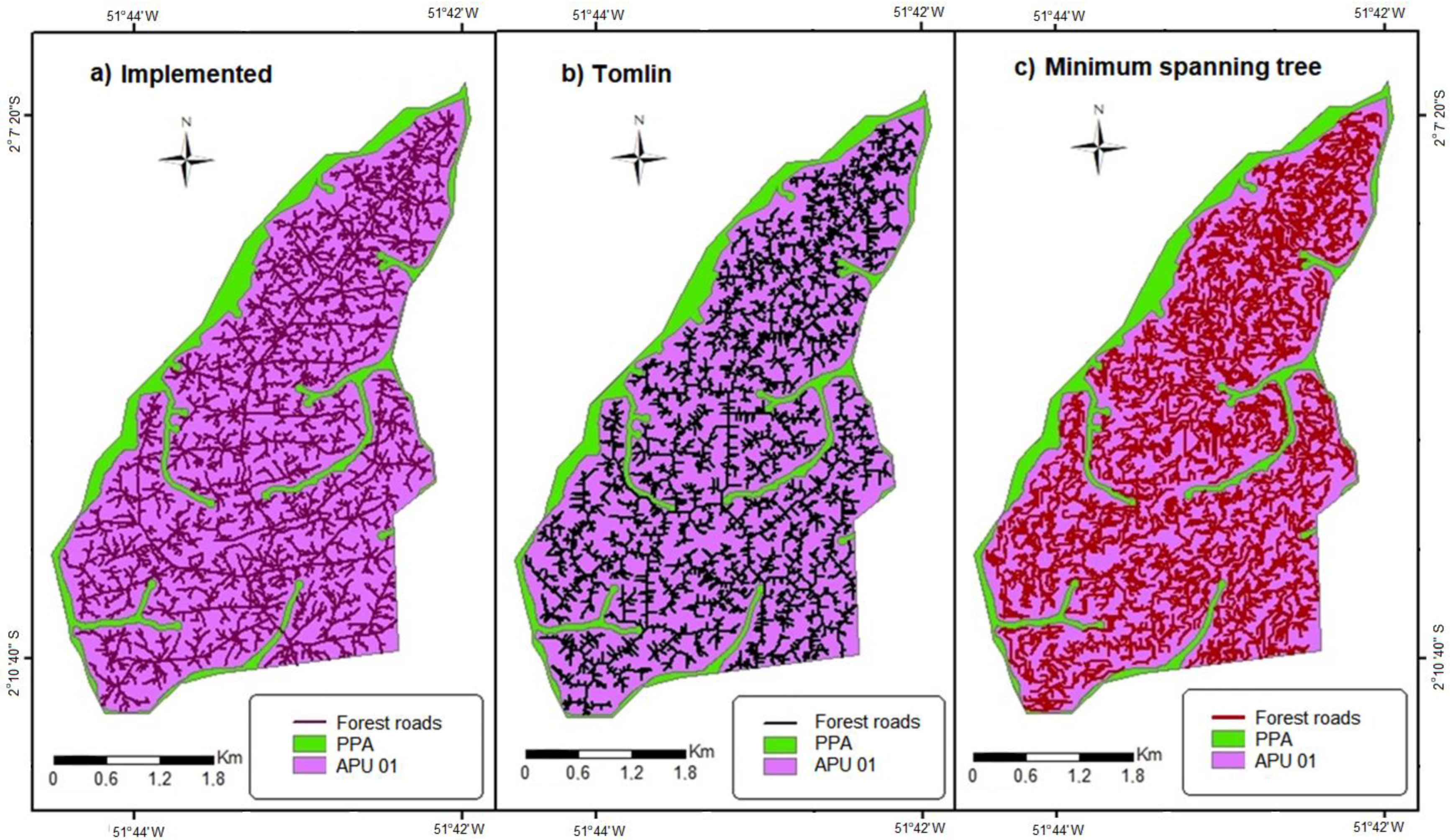
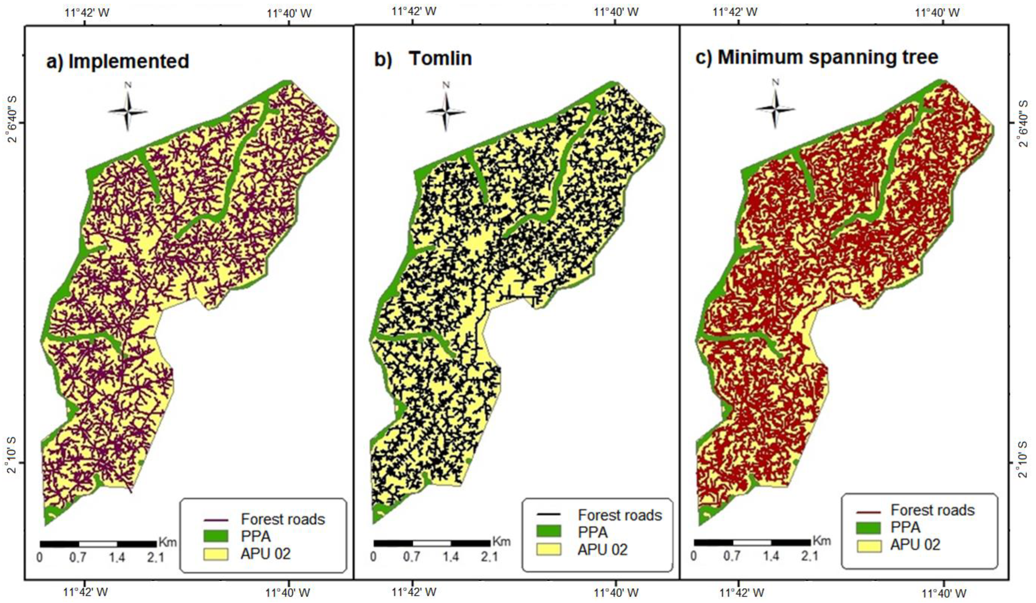
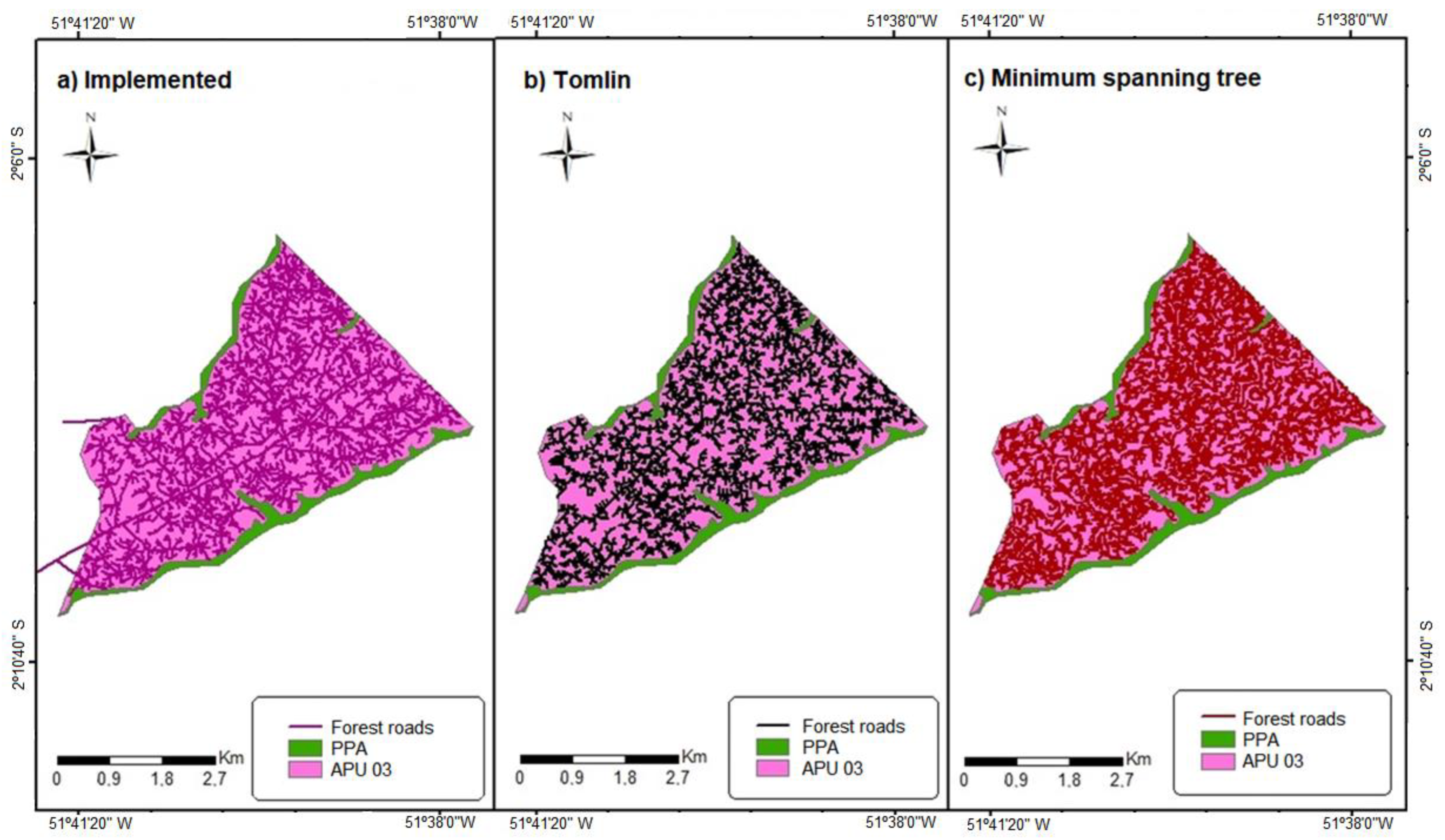
3.1. Road Modeling Based on Location of the Log-Storage
3.2. Road Modeling Based on the Location of the Selectively Logged Trees
3.3. Optimum Road Density (ORD) Determination
4. Discussion
5. Conclusions
Author Contributions
Funding
Institutional Review Board Statement
Informed Consent Statement
Data Availability Statement
Acknowledgments
Conflicts of Interest
References
- Stragliotto, M.C.; Pereira, B.L.C.; Oliveira, A.C. Indústrias Madeireiras e Rendimento em Madeira Serrada na Amazônia Brasileira. In Engenharia Florestal: Desafios, Limites e Potencialidade; Digital, C., Ed.; Científica Digital: São Paulo, Brazil, 2020; Chapter 39; pp. 499–518. [Google Scholar] [CrossRef]
- Rodrigues, M.I.; de Souza, N.; Joaquim, M.S.; Junior, I.M.L.; Pereira, R.S. Concessão florestal na Amazônia brasileira. Ciência Florestal. 2020, 30, 1299–1308. [Google Scholar] [CrossRef]
- Verissimo, A.; Barreto, P.; Mattos, M.; Tarifa, R.; Uhl, C. Logging impacts and prospects for sustainable forest management in an old Amazonian frontier: The case of Paragominas. For. Ecol. Manag. 1992, 55, 169–199. [Google Scholar] [CrossRef]
- Johns, J.S.; Barreto, P.; Uhl, C. Logging damage during planned and unplanned logging operations in the eastern Amazon. For. Ecol. Manag. 1996, 89, 59–77. [Google Scholar] [CrossRef]
- Pereira, R.; Zweede, J.; Asner, G.P.; Keller, M. Forest canopy damage and recovery in reduced-impact and conventional selective logging in eastern Para, Brazil. For. Ecol. Manag. 2002, 168, 77–89. [Google Scholar] [CrossRef]
- Putz, F.; Sist, P.; Fredericksen, T.; Dykstra, D. Reduced-impact logging: Challenges and opportunities. For. Ecol. Manag. 2008, 256, 1427–1433. [Google Scholar] [CrossRef]
- Pinard, M.A.; Putz, F.E. Retaining forest biomass by reducing logging damage. Biotropica 1996, 28, 278–295. [Google Scholar] [CrossRef]
- Azevedo-Ramos, C.; Silva, J.N.M.; Merry, F. The Evolution of Brazilian forest concessions. Elem. Sci. Anthr. 2015, 3, 000048. [Google Scholar] [CrossRef]
- Asner, G.P.; Keller, M.; Lentini, M.; Merry, F.; Souza, C. Selective logging and its relation to deforestation. Amazon. Glob. Chang. 2009, 186, 43–60. [Google Scholar] [CrossRef]
- Matricardi, E.A.; Skole, D.L.; Pedlowski, M.A.; Chomentowski, W.; Fernandes, L.C. Assessment of tropical forest degradation by selective logging and fire using Landsat imagery. Remote Sens. Environ. 2010, 114, 1117–1129. [Google Scholar] [CrossRef]
- Matricardi, E.A.; Skole, D.L.; Pedlowski, M.A.; Chomentowski, W. Assessment of forest disturbances by selective logging and forest fires in the Brazilian Amazon using Landsat data. Int. J. Remote Sens. 2013, 34, 1057–1086. [Google Scholar] [CrossRef]
- Miguel, E.P.; Rezende, A.V.; Leal, F.A.; Matricardi, E.A.T.; Vale, A.T.D.; Pereira, R.S. Artificial neurais networks for modeling wood volume and aboveground biomass of tall Cerrado using satellite data. Pesqui. Agropecuária Bras. 2015, 50, 829–839. [Google Scholar] [CrossRef]
- Pinagé, E.R.; Matricardi, E.A.T. Detection of logging infrastructure in the state of Rondônia using remotely sensed data. Floresta Ambiente 2015, 22, 377–390. [Google Scholar] [CrossRef][Green Version]
- Matricardi, E.A.T.; Skole, D.L.; Costa, O.B.; Pedlowski, M.A.; Samek, J.H.; Miguel, E.P.; Power, S.; Lengaigne, M.; Saitou, M.; Hayashi, K.; et al. Long-term forest degradation surpasses deforestation in the Brazilian Amazon. Science 2020, 369, 1378–1382. [Google Scholar] [CrossRef] [PubMed]
- Kolkos, G.; Stergiadou, A.; Kantartzis, A.; Tampekis, S.; Arabatzis, G. Effects of forest roads and an assessment of their disturbance of the natural enviroment based on GIS spatial multi-criteria analysis: Case study of the University Forest of Taxiarchis, Chalkidiki, Greece. Euro-Mediterr. J. Environ. Integr. 2023, 8, 425–440. [Google Scholar] [CrossRef]
- Miller, S.D.; Goulden, M.L.; Hutyra, L.R.; Keller, M.; Saleska, S.R.; Wofsy, S.C.; Figueira, A.M.S.; da Rocha, H.R.; de Camargo, P.B. Reduced impact logging minimally alters tropical rainforest carbon and energy exchange. Proc. Natl. Acad. Sci. USA 2011, 108, 19431–19435. [Google Scholar] [CrossRef]
- Espada, A.L.V.; Pires, I.P.; Lentini, M.A.; Bittencourt, P.R. Manejo florestal e exploração de impacto reduzido em florestas naturais de produção da Amazônia. Inst. Floresta Trop. 2016, 32. Available online: https://ift.org.br/wp-content/uploads/2014/11/Informativo-T%C3%A9cnico-1.pdf (accessed on 2 May 2023).
- Zagonel, R.; Corrêa, C.M.C.; Malinovski, J.R. Optimal forest road density in plane relief in Pinus taeda forests in Catarinense plateaus. Sci. For. 2008, 36, 33–41. Available online: https://www.ipef.br/publicacoes/scientia/nr77/cap04.pdf (accessed on 2 May 2023).
- Braz, E.M.; Oliveira, M.V.N. Planejamento de arraste mecanizado em floresta tropical. Embrapa CPAF-AC Rio Branco AC 1997, 5, 6. Available online: https://www.infoteca.cnptia.embrapa.br/infoteca/bitstream/doc/492550/1/it05.pdf (accessed on 2 May 2023).
- Rogers, L.; Schiess, P. PEGGER & ROADVIEW—A New GIS Tool To Assist Engineers in Operations Planning. In Proceedings of the Internacional Mountain Logging and 11th Pacific Northwest Skyline Symposium, Seattle, WA, USA, 10–12 December 2001; pp. 177–182. Available online: https://depts.washington.edu/sky2001/proceedings/papers/Rogers.pdf (accessed on 2 May 2023).
- Tomlin, C.D. Geographic Information Systems and Cartographic Modeling; Prentice Hall Press: Hoboken, NJ, USA, 1990; 572p. [Google Scholar]
- Wallis, W.D. A Beginner’s Guide to Graph Theory; Springer Science Business Media Press: Berlin/Heidelberg, Germany, 2000; 244p, Available online: https://link.springer.com/book/10.1007/978-1-4757-3134-7 (accessed on 2 May 2023).
- Caixeta-Filho, J.V. Pesquisa Operacional: Técnicas de Otimização Aplicadas a Sistemas Agroindustriais, 2nd ed.; Atlas Press: São Paulo, Brazil, 2004; 176p. [Google Scholar]
- PRIM, R.C. Shortest Connection Networks and Some Generalizations. Bell Syst. Tech. J. 1957, 36, 1389–1401. [Google Scholar] [CrossRef]
- Ivanov, A.O.; Tuzhilin, A.A. Minimal Networks the Steiner Problem and Its Generalizations; CRC Press: Boca Raton, FL, USA, 1994. [Google Scholar]
- ICMBIO—Chico Mendes Institute of Biodiversity Conservation. PMF—Plano e Manejo da Floresta Nacional de Caxiuanã, Volume I—Diagnóstico. Instituto Chico Mendes de Conservação da Biodiversidade (ICMBio), Brasília, Brazil. 2012. Available online: https://www.gov.br/icmbio/pt-br/assuntos/biodiversidade/unidade-de-conservacao/unidades-de-biomas/amazonia/lista-de-ucs/flona-de-caxiuana/arquivos/volumeI_completo.pdf (accessed on 2 May 2023).
- CEMAL—Comércio Ecológico de Madeiras Ltda. Plano de Manejo Florestal Sustentável Pracupi, UMF III, Flona de Caxiuanã. Syr. Stud. 2022, 7, 122. [Google Scholar]
- Oliveira, L.D.; Cunha, A.C.; Costa, A.C.L.; Costa, R.F. Sazonalidade e interceptação da chuva na Floresta Nacional em Caxiuanã—Amazônia Oriental. Sci. Plena 2011, 7, 285–294. [Google Scholar]
- Veríssimo, A.; Barreto, P.; Tarifa, R.; Uhl, C. Extraction of a high-value natural resource in Amazonia: The case of mahogany. For. Ecol. Manag. 1995, 72, 39–60. [Google Scholar] [CrossRef]
- Arima, E.Y.; Walker, R.T.; Sales, M.; Souza, C.; Perz, S.G. The fragmentation of space in the Amazon basin: Emergent road networks. Photogramm. Eng. Remote Sens. 2008, 74, 699–709. [Google Scholar] [CrossRef]
- Arima, E.Y.; Walker, R.T.; Perz, S.G.; Caldas, M. Loggers and Forest Fragmentation: Behavioral Models of Road Building in the Amazon Basin. Ann. Assoc. Am. Geogr. 2005, 95, 525–541. [Google Scholar] [CrossRef]
- Dijkstra, E.W. A note on two problems in connexion with graphs. In Numerische Mathematik, 1; Springer: Berlin/Heidelberg, Germany, 1959; pp. 269–271. [Google Scholar]
- Shreve, R. Statistical Law of Stream Numbers. J. Geol. 1966, 74, 17–37. [Google Scholar] [CrossRef]
- Malinovski, J.R.; Perdoncini, W.C. Estradas Florestais. Publicação Técnica Colégio Irati GTZ 1990, 100. [Google Scholar]
- Machado, C.C.; Malinovski, J.R. Ciência do Trabalho Florestal; UFV Press: Viçosa, Brazil, 1988; 65p. [Google Scholar]
- Malinovski, R.A. Densidades aceitáveis de estradas. In Proceedings of the Annals of Encontro Brasileiro De Infraestrutura Florestal, Curitiba, Brazil, 2013. [Google Scholar]
- Souza, F.L.; Sampietro, J.A.; Dacoregio, H.M.; Soares, P.R.C.; Lopes, E.D.S.; Quadros, D.S. Optimum and acceptable forest road density in pine harvesting for cut-to-length and full tree systems. Sci. For. 2018, 118, 189–198. [Google Scholar]


| Annual Production Unit (*) | Area (ha) | Harvesting Year |
|---|---|---|
| 1 | 1828.5 | 2019 |
| 2 | 1951.9 | 2020 |
| 3 | 1949.1 | 2021 |
| Total | 5729.5 |
| Skidding Log | Skidder Costs | ||
|---|---|---|---|
| Extracted logs per day * | 5.00 | Acquisition price (USD) * | 386,220.00 |
| Average log volume (m3) * | 2.5 | Resale value (USD) ** | 77,243.20 |
| Working hours per day * | 8.00 | Estimate lifespan (year) ** | 25.00 |
| * Dataset provided by [27] ** Data from current scientific literature | Fuel consumption (L·h−1) * | 14.00 | |
| Diesel price (USD/L) | 1.35 | ||
| Hydraulic oil consumption (L·h−1) ** | 0.21 | ||
| Hydraulic oil price (USD/L) | 6.76 | ||
| Motor oil consumption (L·h−1) ** | 0.13 | ||
| Motor oil price (USD/L) | 3.28 | ||
| Tire price (USD/unit) ** | 2793.10 | ||
| Tire lifespan (hour)** | 2500.00 | ||
| Wage (USD/months) ** | 391.60 | ||
| APU * | Models | Area (Hectares) | Bridges | ||
|---|---|---|---|---|---|
| Main Roads | Secondary Roads | Impacted PPA ** | |||
| 01 | Planned | 7.32 | 27.41 | 0.11 | 1 |
| Implemented | 8.14 | 25.41 | 0.10 | 1 | |
| Tomlin | 12.09 | 26.62 | 0 | 0 | |
| Minimum Spanning tree | 14.14 | 32.20 | 0 | 0 | |
| 02 | Planned | 7.99 | 30.11 | 0 | 0 |
| Implemented | 8.54 | 26.50 | 0.15 | 1 | |
| Tomlin | 8.77 | 30.24 | 0 | 0 | |
| Minimum Spanning tree | 13.45 | 39.89 | 0 | 0 | |
| 03 | Planned | 6.22 | 29.60 | 0 | 0 |
| Implemented | 6.77 | 29.52 | 0 | 0 | |
| Tomlin | 8.99 | 33.23 | 0 | 0 | |
| Minimum Spanning tree | 15.04 | 39.86 | 0 | 0 | |
| APU * | Total Length of Roads and Skid Trails (Meters) | ||
|---|---|---|---|
| Field-Implemented | Tomlin | Minimum Spanning Tree | |
| 01 | 232,640.1 | 249,376.7 | 431,715.2 |
| 02 | 286,268.0 | 324,140.0 | 564,977.3 |
| 03 | 266,895.6 | 283,017.1 | 498,923.0 |
| Modeling Approach | Cext | Croad | Cdeg | CTot | RD | ASD | RS |
|---|---|---|---|---|---|---|---|
| USD m−3 | m.ha−1 | m | m | ||||
| Planned | 8.33 | 4.48 | 1.40 | 14.21 | 18.83 | 248.94 | 573.15 |
| Field-implemented | 8.52 | 4.16 | 1.30 | 13.98 | 17.48 | 268.16 | 607.03 |
| Tomlin model | 8.38 | 4.40 | 1.37 | 14.15 | 18.47 | 253.79 | 589.41 |
| Spanning tree model | 7.93 | 5.36 | 1.67 | 14.97 | 22.51 | 208.24 | 589.41 |
| Optimum | 9.68 | 2.89 | 0.90 | 13.47 | 12.11 | 386.98 | 825.37 |
| Acceptable | 8.39 | 4.38 | 1.37 | 14.14 | 18.41 | 254.62 | 543.18 |
| Modeling Approach | Cext | Croad | Cdeg | CTot | RD | ASD | RS |
|---|---|---|---|---|---|---|---|
| USD m−3 | m·ha−1 | m | m | ||||
| Planned | 8.27 | 4.61 | 1.44 | 14.32 | 19.36 | 242.12 | 569.21 |
| Field-implemented | 8.59 | 4.06 | 1.27 | 13.91 | 17.05 | 274.93 | 589.41 |
| Tomlin model | 8.25 | 4.65 | 1.45 | 14.34 | 19.51 | 240.26 | 597.75 |
| Spanning tree model | 7.66 | 6.20 | 1.93 | 15.79 | 26.03 | 180.08 | 597.75 |
| Optimum | 9.68 | 2.89 | 0.90 | 13.47 | 12.11 | 386.98 | 825.37 |
| Acceptable | 8.39 | 4.38 | 1.37 | 14.14 | 18.41 | 254.62 | 543.18 |
| Modeling Approach | Cext | Croad | Cdeg | CTot | RD | ASD | RS |
|---|---|---|---|---|---|---|---|
| USD m−3 | m·ha−1 | m | m | ||||
| Planned | 8.30 | 4.54 | 1.42 | 14.26 | 19.06 | 245.93 | 732.39 |
| Field-implemented | 8.31 | 4.52 | 1.41 | 14.25 | 19.00 | 246.71 | 1190.97 |
| Tomlin model | 8.00 | 5.18 | 1.62 | 14.81 | 21.77 | 215.32 | 960.47 |
| Spanning tree model | 7.66 | 6.18 | 1.93 | 15.78 | 25.97 | 180.5 | 960.49 |
| Optimum | 9.68 | 2.89 | 0.90 | 13.47 | 12.11 | 386.98 | 825.37 |
| Acceptable | 8.39 | 4.38 | 1.37 | 14.14 | 18.41 | 254.62 | 543.18 |
Disclaimer/Publisher’s Note: The statements, opinions and data contained in all publications are solely those of the individual author(s) and contributor(s) and not of MDPI and/or the editor(s). MDPI and/or the editor(s) disclaim responsibility for any injury to people or property resulting from any ideas, methods, instructions or products referred to in the content. |
© 2023 by the authors. Licensee MDPI, Basel, Switzerland. This article is an open access article distributed under the terms and conditions of the Creative Commons Attribution (CC BY) license (https://creativecommons.org/licenses/by/4.0/).
Share and Cite
Morais, P.d.P.; Arima, E.Y.; de Souza, Á.N.; Pereira, R.S.; Emmert, F.; Cardoso, R.M.; Miguel, E.P.; Matricardi, E.A.T. Assessment of Forest Road Models in Concession Areas in the Brazilian Amazon. Forests 2023, 14, 1388. https://doi.org/10.3390/f14071388
Morais PdP, Arima EY, de Souza ÁN, Pereira RS, Emmert F, Cardoso RM, Miguel EP, Matricardi EAT. Assessment of Forest Road Models in Concession Areas in the Brazilian Amazon. Forests. 2023; 14(7):1388. https://doi.org/10.3390/f14071388
Chicago/Turabian StyleMorais, Pricila do Prado, Eugenio Yatsuda Arima, Álvaro Nogueira de Souza, Reginaldo Sérgio Pereira, Fabiano Emmert, Rodrigo Montezano Cardoso, Eder Pereira Miguel, and Eraldo Aparecido Trondoli Matricardi. 2023. "Assessment of Forest Road Models in Concession Areas in the Brazilian Amazon" Forests 14, no. 7: 1388. https://doi.org/10.3390/f14071388
APA StyleMorais, P. d. P., Arima, E. Y., de Souza, Á. N., Pereira, R. S., Emmert, F., Cardoso, R. M., Miguel, E. P., & Matricardi, E. A. T. (2023). Assessment of Forest Road Models in Concession Areas in the Brazilian Amazon. Forests, 14(7), 1388. https://doi.org/10.3390/f14071388