


Wildfire Susceptibility Mapping Using Deep Learning Algorithms in Two Satellite Imagery Dataset


 , ,
, ,  ,
,
Abstract
1. Introduction
2. Materials and Methods
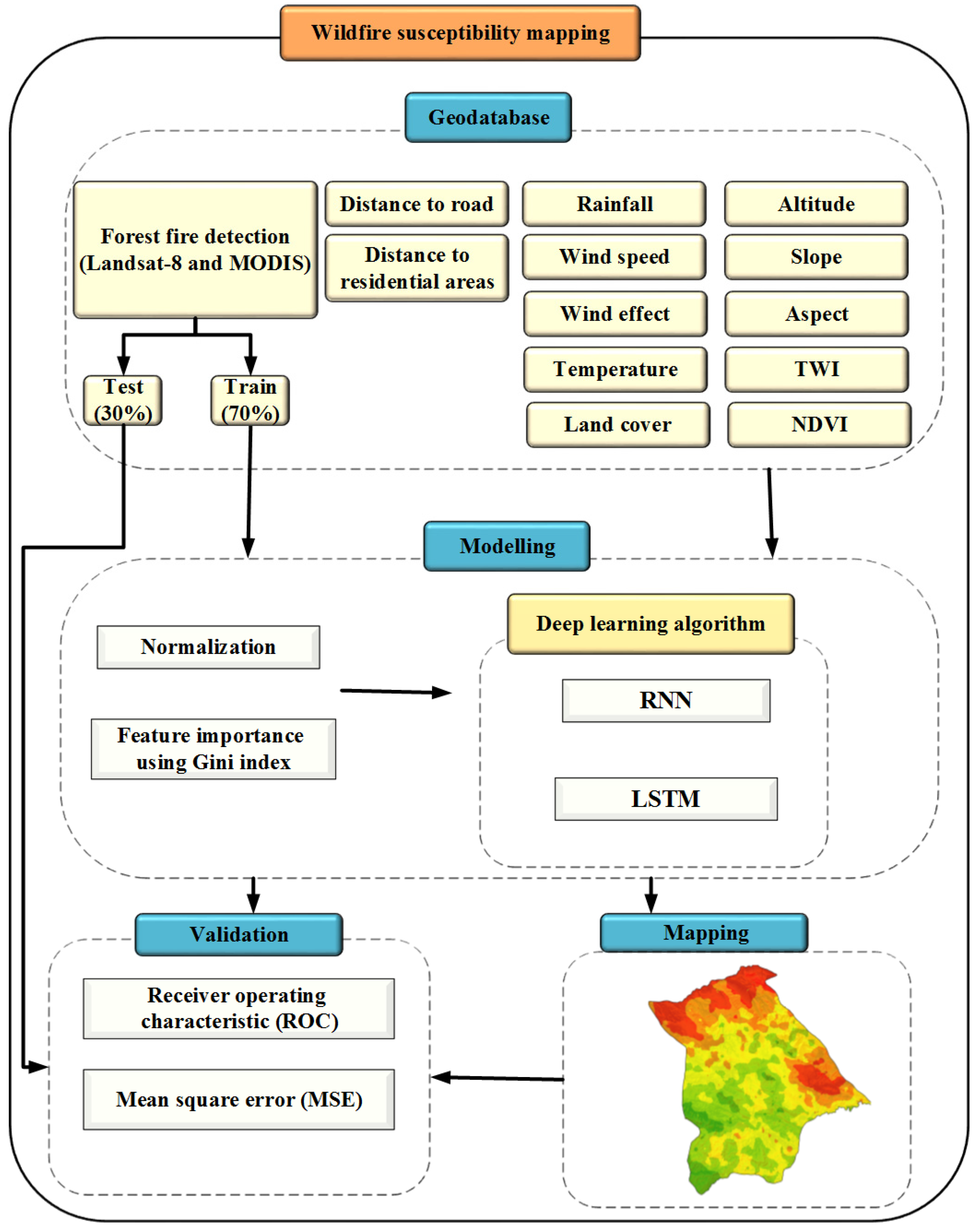
2.1. Methodology
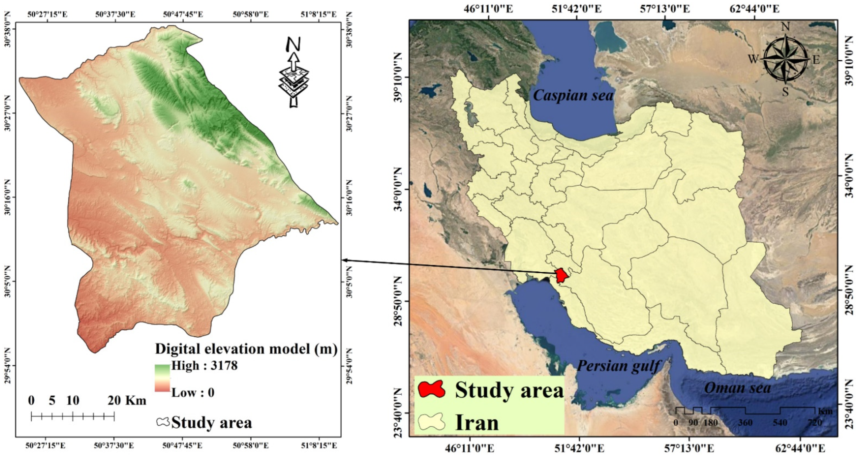
2.2. Study Area
2.3. Data
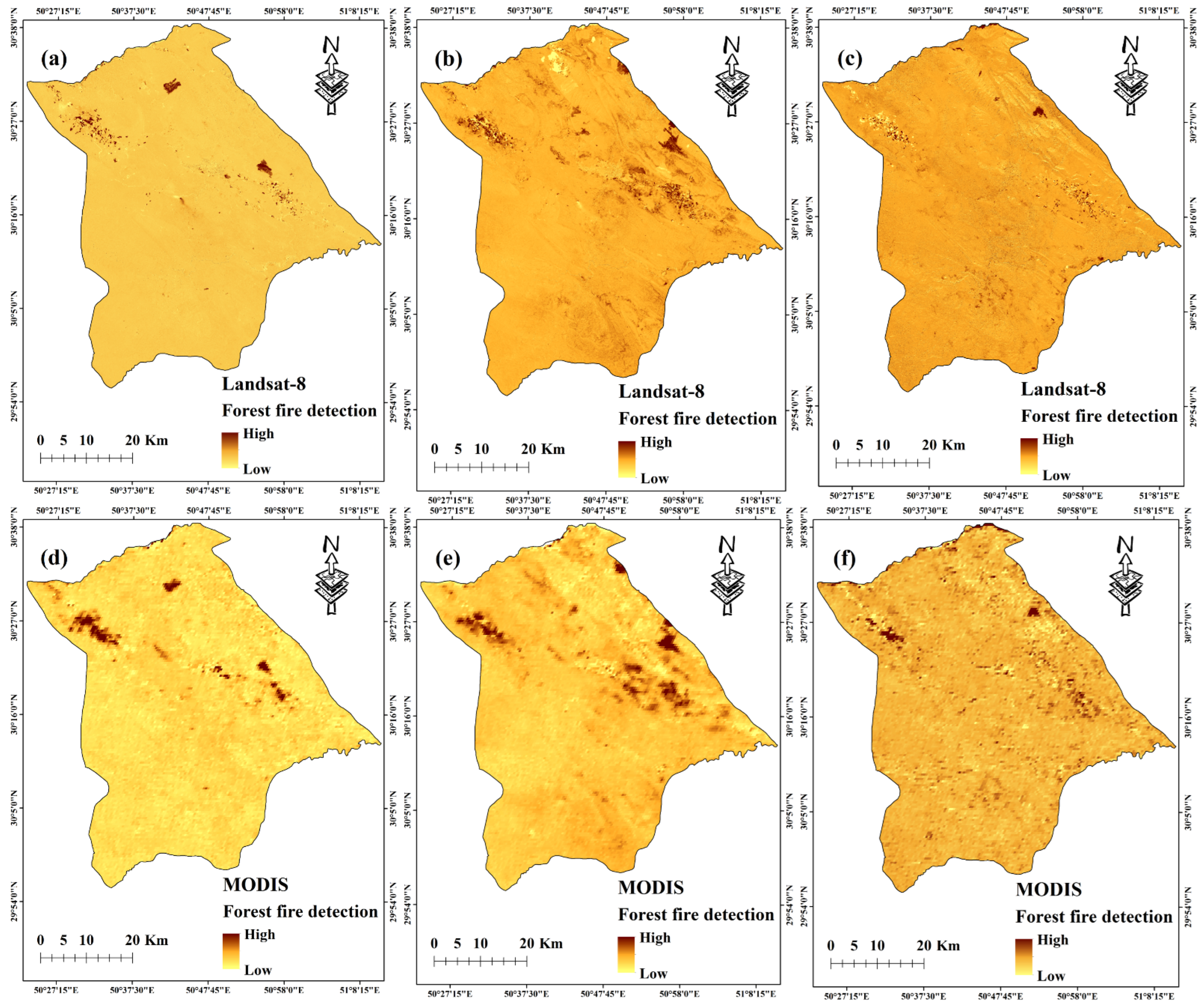
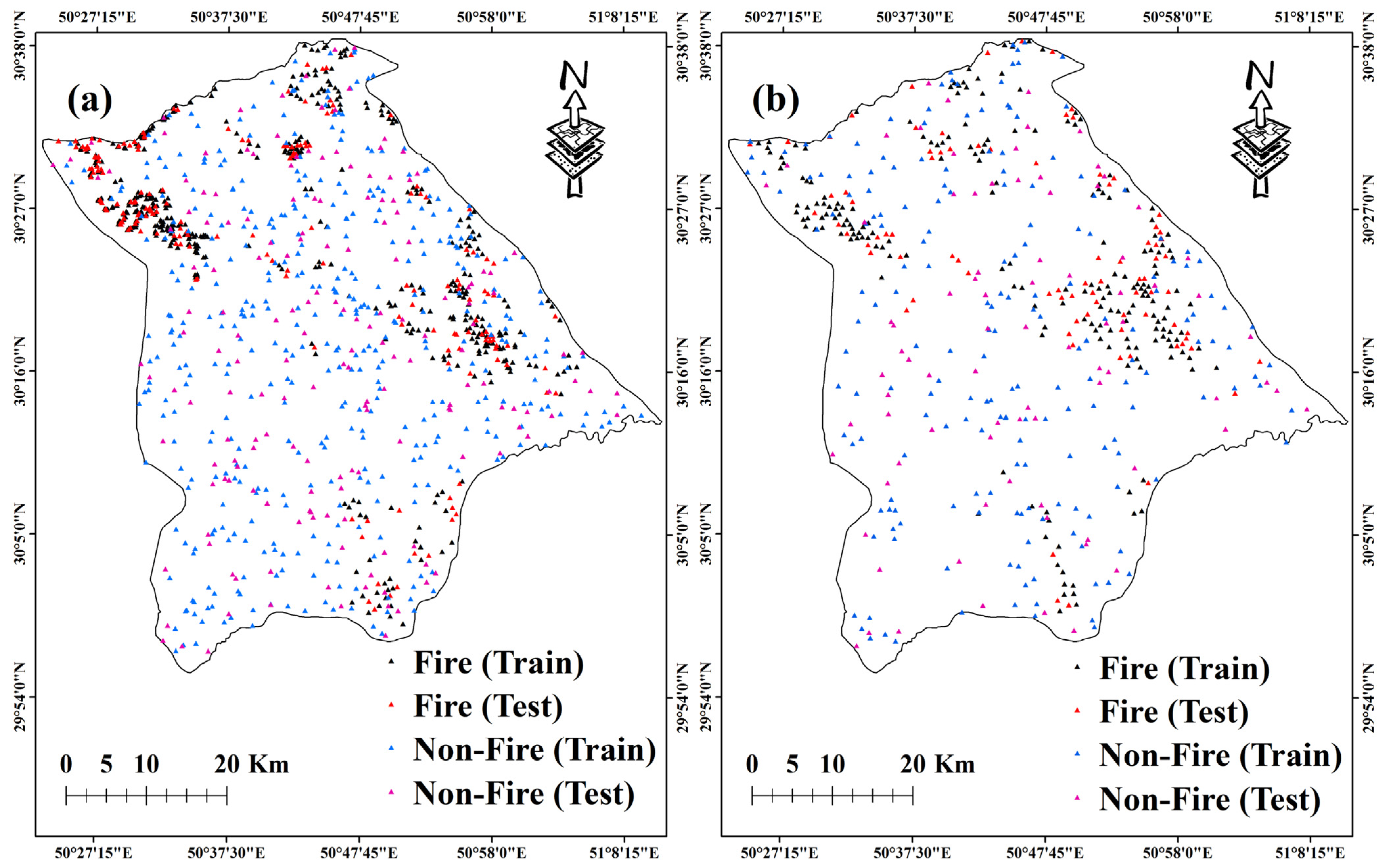
2.3.1. Previous Wildfires
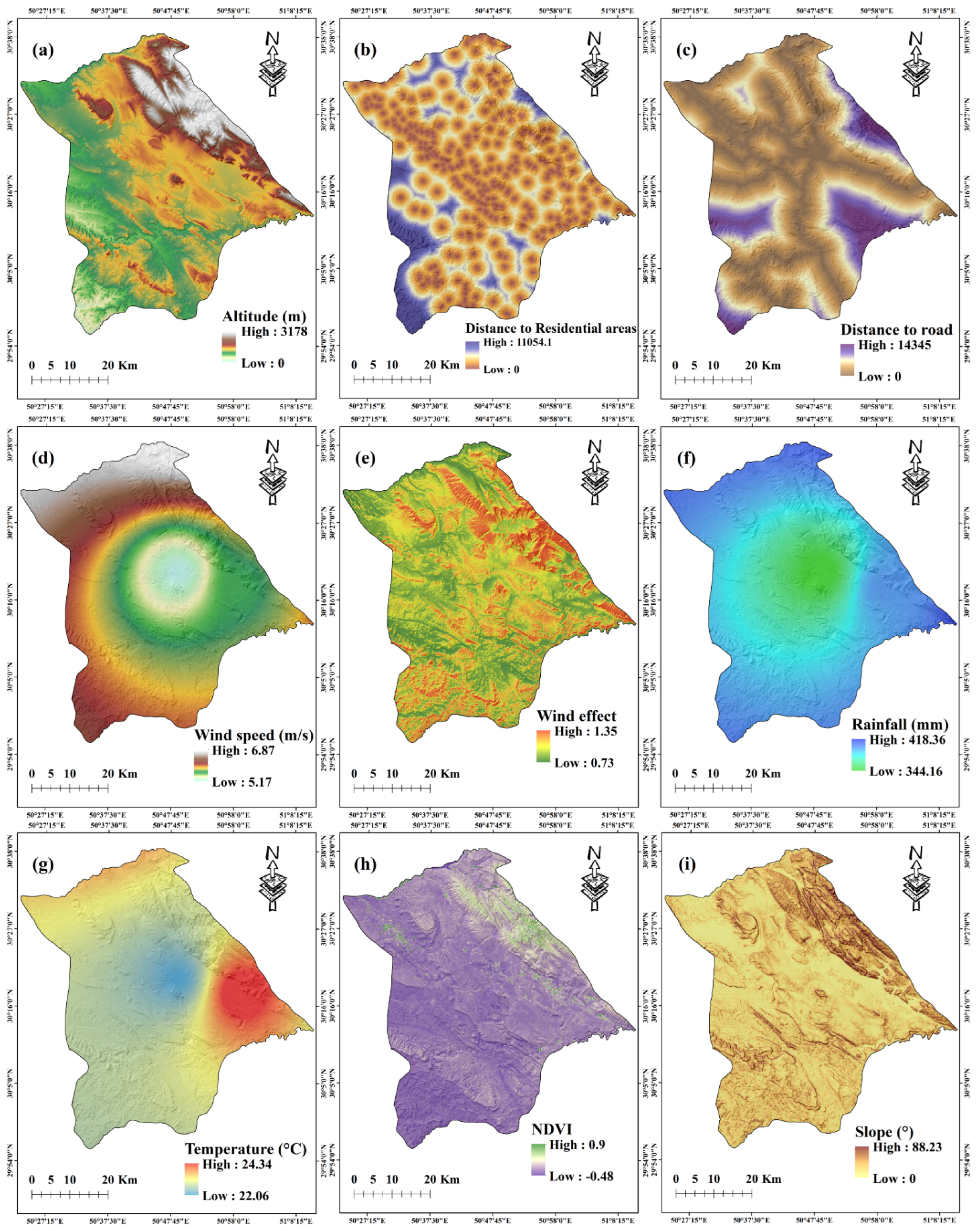
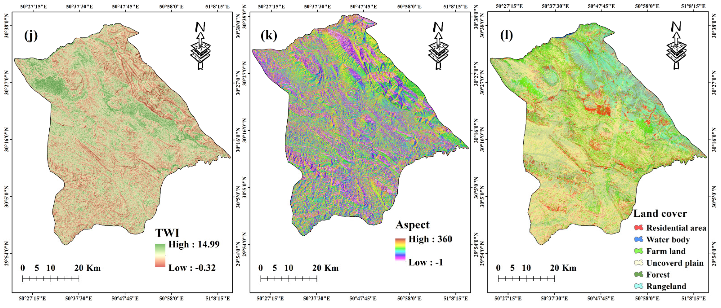
2.3.2. Effective Factors
2.4. Wildfire Susceptibility Methods
2.4.1. Recurrent Neural Network (RNN)
2.4.2. Long Short-Term Memory (LSTM)
2.4.3. Multicollinearity Analysis
2.4.4. Feature Importance Using Gini Index
2.4.5. Validation
- MSE
- ROC and AUC
3. Results
3.1. Result of Multicollinearity
3.2. Determining the Importance of Factors Affecting Wildfires
3.3. Wildfire Susceptibility Modeling with Deep Learning Algorithms
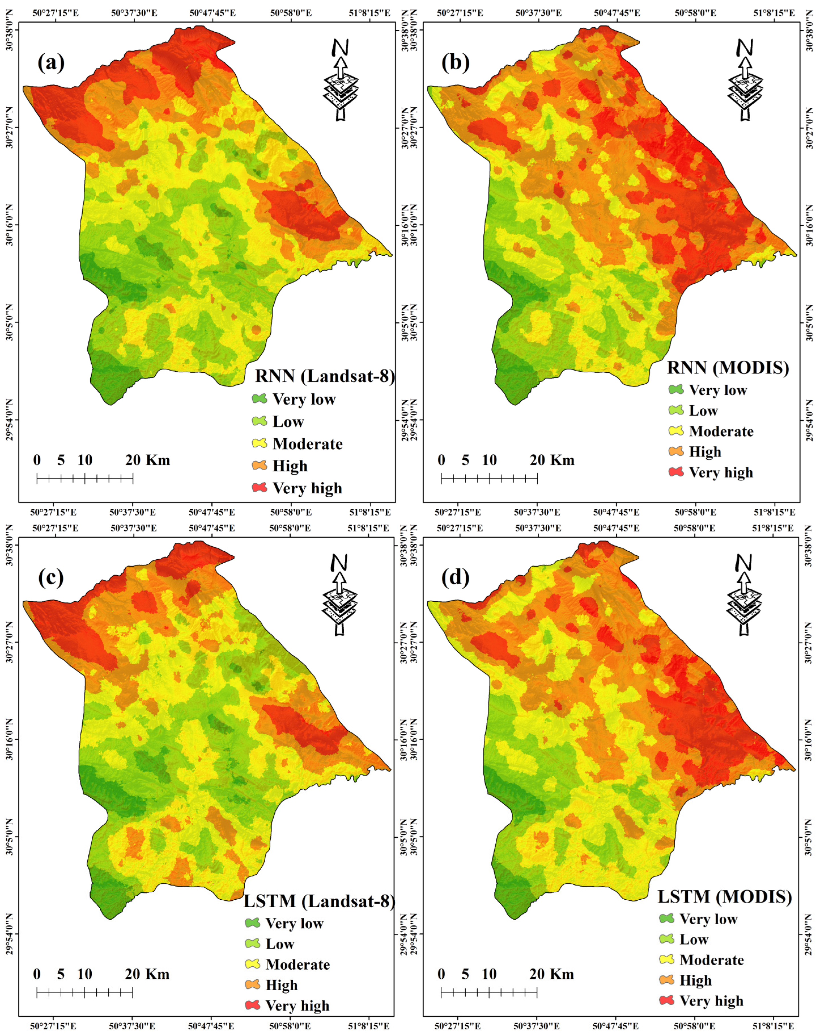
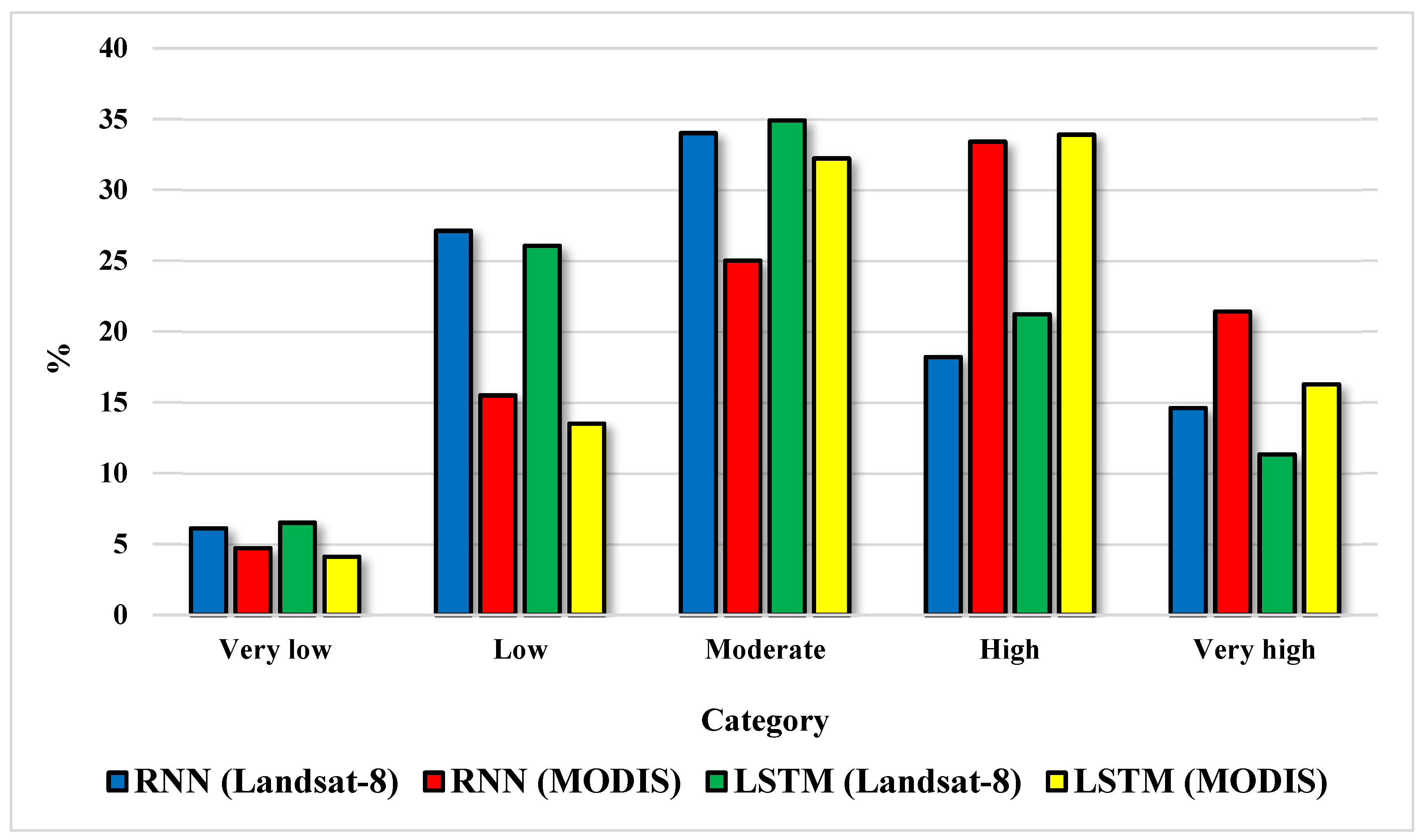
3.4. Wildfire Susceptibility Mapping
3.5. Validation of Models and Susceptibility Maps
4. Discussion
Limitations and Future Recommendations
5. Conclusions
Author Contributions
Funding
Institutional Review Board Statement
Informed Consent Statement
Data Availability Statement
Conflicts of Interest
References
- Oom, D.; Pereira, J.M. Exploratory spatial data analysis of global MODIS active fire data. Int. J. Appl. Earth Obs. Geoinf. 2013, 21, 326–340. [Google Scholar] [CrossRef]
- Hantson, S.; Pueyo, S.; Chuvieco, E. Global fire size distribution: From power law to log-normal. Int. J. Wildland Fire 2016, 25, 403–412. [Google Scholar] [CrossRef]
- Li, J.; Shan, Y.; Yin, S.; Wang, M.; Sun, L.; Wang, D. Nonparametric multivariate analysis of variance for affecting factors on the extent of wildfire damage in Jilin Province, China. J. For. Res. 2019, 30, 2185–2197. [Google Scholar] [CrossRef]
- Zema, D.A.; Nunes, J.P.; Lucas-Borja, M.E. Improvement of seasonal runoff and soil loss predictions by the MMF (Morgan-Morgan-Finney) model after wildfire and soil treatment in Mediterranean forest ecosystems. Catena 2020, 188, 104415. [Google Scholar] [CrossRef]
- Santana, V.M.; Alday, J.G.; Baeza, M.J. Mulch application as post-fire rehabilitation treatment does not affect vegetation recovery in ecosystems dominated by obligate seeders. Ecol. Eng. 2014, 71, 80–86. [Google Scholar] [CrossRef]
- Adab, H.; Kanniah, K.D.; Solaimani, K. Modeling wildfire risk in the northeast of Iran using remote sensing and GIS techniques. Nat. Hazards 2013, 65, 1723–1743. [Google Scholar] [CrossRef]
- Shiravand, H.; Hosseini, S.A. A new evaluation of the influence of climate change on Zagros oak forest dieback in Iran. Theor. Appl. Climatol. 2020, 141, 685–697. [Google Scholar] [CrossRef]
- Feizizadeh, B.; Omarzadeh, D.; Mohammadnejad, V.; Khallaghi, H.; Sharifi, A.; Karkarg, B.G. An integrated approach of artificial intelligence and geoinformation techniques applied to wildfire risk modeling in Gachsaran, Iran. J. Environ. Plan. Manag. 2023, 66, 1369–1391. [Google Scholar] [CrossRef]
- Jaafari, A.; Termeh, S.V.R.; Bui, D.T. Genetic and firefly metaheuristic algorithms for an optimized neuro-fuzzy prediction modeling of wildfire probability. J. Environ. Manag. 2019, 243, 358–369. [Google Scholar] [CrossRef] [PubMed]
- Adab, H. Landfire hazard assessment in the Caspian Hyrcanian forest ecoregion with the long-term MODIS active fire data. Nat. Hazards 2017, 87, 1807–1825. [Google Scholar] [CrossRef]
- Xu, R.; Lin, H.; Lu, K.; Cao, L.; Liu, Y. A wildfire detection system based on ensemble learning. Forests 2021, 12, 217. [Google Scholar] [CrossRef]
- Zhang, J.; Li, W.; Yin, Z.; Liu, S.; Guo, X. Wildfire detection system based on wireless sensor network. In Proceedings of the 2009 4th IEEE Conference on Industrial Electronics and Applications, Xi’an, China, 25–27 May 2009; pp. 520–523. [Google Scholar]
- Yu, L.; Wang, N.; Meng, X. Real-time wildfire detection with wireless sensor networks. In Proceedings of the 2005 International Conference on Wireless Communications, Networking and Mobile Computing, Wuhan, China, 26 September 2005; pp. 1214–1217. [Google Scholar]
- Chen, S.-J.; Hovde, D.C.; Peterson, K.A.; Marshall, A.W. Fire detection using smoke and gas sensors. Fire Saf. J. 2007, 42, 507–515. [Google Scholar] [CrossRef]
- Lee, B.; Kwon, O.; Jung, C.; Park, S. The development of UV/IR combination flame detector. J. KIIS 2001, 16, 140–145. [Google Scholar]
- Kang, D.; Kim, E.; Moon, P.; Sin, W.; Kang, M.-g. Design and analysis of flame signal detection with the combination of UV/IR sensors. J. Internet Comput. Serv. 2013, 14, 45–51. [Google Scholar] [CrossRef]
- Hendel, I.-G.; Ross, G.M. Efficacy of remote sensing in early wildfire detection: A thermal sensor comparison. Can. J. Remote Sens. 2020, 46, 414–428. [Google Scholar] [CrossRef]
- Varotsos, C.A.; Krapivin, V.F.; Mkrtchyan, F.A. A new passive microwave tool for operational wildfires detection: A case study of siberia in 2019. Remote Sens. 2020, 12, 835. [Google Scholar] [CrossRef]
- Pradhan, B.; Al-Najjar, H.A.; Sameen, M.I.; Tsang, I.; Alamri, A.M. Unseen land cover classification from high-resolution orthophotos using integration of zero-shot learning and convolutional neural networks. Remote Sens. 2020, 12, 1676. [Google Scholar] [CrossRef]
- Gibril, M.B.A.; Kalantar, B.; Al-Ruzouq, R.; Ueda, N.; Saeidi, V.; Shanableh, A.; Mansor, S.; Shafri, H.Z. Mapping heterogeneous urban landscapes from the fusion of digital surface model and unmanned aerial vehicle-based images using adaptive multiscale image segmentation and classification. Remote Sens. 2020, 12, 1081. [Google Scholar] [CrossRef]
- You, W.; Lin, L.; Wu, L.; Ji, Z.; Zhu, J.; Fan, Y.; He, D. Geographical information system-based wildfire risk assessment integrating national forest inventory data and analysis of its spatiotemporal variability. Ecol. Indic. 2017, 77, 176–184. [Google Scholar] [CrossRef]
- Fernandes, A.M.; Utkin, A.B.; Lavrov, A.V.; Vilar, R.M. Development of neural network committee machines for automatic wildfire detection using lidar. Pattern Recognit. 2004, 37, 2039–2047. [Google Scholar] [CrossRef]
- Jaiswal, R.K.; Mukherjee, S.; Raju, K.D.; Saxena, R. Wildfire risk zone mapping from satellite imagery and GIS. Int. J. Appl. Earth Obs. Geoinf. 2002, 4, 1–10. [Google Scholar]
- Erten, E.; Kurgun, V.; Musaoglu, N. Wildfire risk zone mapping from satellite imagery and GIS: A case study. In Proceedings of the XXth Congress of the International Society for Photogrammetry and Remote Sensing, Istanbul, Turkey, 15 July 2004; pp. 222–230. [Google Scholar]
- Pradhan, B.; Awang, M.A. Application of remote sensing and gis for wildfire susceptibility mapping using likelihood ratio model. Proc. Map Malays. 2007, 16, 3. [Google Scholar]
- Schroeder, W.; Oliva, P.; Giglio, L.; Quayle, B.; Lorenz, E.; Morelli, F. Active fire detection using Landsat-8/OLI data. Remote Sens. Environ. 2016, 185, 210–220. [Google Scholar] [CrossRef]
- Zhang, T.; Wooster, M.J.; Xu, W. Approaches for synergistically exploiting VIIRS I-and M-Band data in regional active fire detection and FRP assessment: A demonstration with respect to agricultural residue burning in Eastern China. Remote Sens. Environ. 2017, 198, 407–424. [Google Scholar] [CrossRef]
- Gargiulo, M. Advances on CNN-based super-resolution of Sentinel-2 images. In Proceedings of the IGARSS 2019–2019 IEEE International Geoscience and Remote Sensing Symposium, Yokohama, Japan, 28 July–2 August 2019; pp. 3165–3168. [Google Scholar]
- Konkathi, P.; Shetty, A. Inter comparison of post-fire burn severity indices of Landsat-8 and Sentinel-2 imagery using Google Earth Engine. Earth Sci. Inform. 2021, 14, 645–653. [Google Scholar] [CrossRef]
- Lyon, J.G.; Yuan, D.; Lunetta, R.S.; Elvidge, C.D. A change detection experiment using vegetation indices. Photogramm. Eng. Remote Sens. 1998, 64, 143–150. [Google Scholar]
- Shang, X.; Song, M.; Wang, Y.; Yu, C.; Yu, H.; Li, F.; Chang, C.-I. Target-constrained interference-minimized band selection for hyperspectral target detection. IEEE Trans. Geosci. Remote Sens. 2020, 59, 6044–6064. [Google Scholar] [CrossRef]
- Wang, P.; Wang, L.; Leung, H.; Zhang, G. Super-resolution mapping based on spatial–spectral correlation for spectral imagery. IEEE Trans. Geosci. Remote Sens. 2020, 59, 2256–2268. [Google Scholar] [CrossRef]
- Pradhan, B.; Suliman, M.D.H.B.; Awang, M.A.B. Wildfire susceptibility and risk mapping using remote sensing and geographical information systems (GIS). Disaster Prev. Manag. Int. J. 2007, 16, 344–352. [Google Scholar] [CrossRef]
- Lin, W.; Zhang, Z.; Zhang, L. Infrared moving small target detection and tracking algorithm based on feature point matching. Eur. Phys. J. D 2022, 76, 185. [Google Scholar] [CrossRef]
- Hwang, C.-L.; Yoon, K. Multiple Attribute Decision Making: Methods and Applications: A State-of-the-Art Survey; Springer: Berlin/Heidelberg, Germany, 1981. [Google Scholar]
- Chatterjee, P.; Chakraborty, S. A comparative analysis of VIKOR method and its variants. Decis. Sci. Lett. 2016, 5, 469–486. [Google Scholar] [CrossRef]
- Goleiji, E.; Hosseini, S.M.; Khorasani, N.; Monavari, S.M. Wildfire risk assessment-an integrated approach based on multicriteria evaluation. Environ. Monit. Assess. 2017, 189, 612. [Google Scholar] [CrossRef]
- Ljubomir, G.; Pamučar, D.; Drobnjak, S.; Pourghasemi, H.R. Modeling the spatial variability of wildfire susceptibility using geographical information systems and the analytical hierarchy process. In Spatial Modeling in GIS and R for Earth and Environmental Sciences; Elsevier: Amsterdam, The Netherlands, 2019; pp. 337–369. [Google Scholar]
- Samui, P. Support vector machine applied to settlement of shallow foundations on cohesionless soils. Comput. Geotech. 2008, 35, 419–427. [Google Scholar] [CrossRef]
- Jaafari, A.; Gholami, D.M.; Zenner, E.K. A Bayesian modeling of wildfire probability in the Zagros Mountains, Iran. Ecol. Inform. 2017, 39, 32–44. [Google Scholar] [CrossRef]
- Hong, H.; Naghibi, S.A.; Moradi Dashtpagerdi, M.; Pourghasemi, H.R.; Chen, W. A comparative assessment between linear and quadratic discriminant analyses (LDA-QDA) with frequency ratio and weights-of-evidence models for wildfire susceptibility mapping in China. Arab. J. Geosci. 2017, 10, 167. [Google Scholar] [CrossRef]
- Abedi Gheshlaghi, H.; Feizizadeh, B.; Blaschke, T. GIS-based wildfire risk mapping using the analytical network process and fuzzy logic. J. Environ. Plan. Manag. 2020, 63, 481–499. [Google Scholar] [CrossRef]
- Nami, M.; Jaafari, A.; Fallah, M.; Nabiuni, S. Spatial prediction of wildfire probability in the Hyrcanian ecoregion using evidential belief function model and GIS. Int. J. Environ. Sci. Technol. 2018, 15, 373–384. [Google Scholar] [CrossRef]
- Ganteaume, A.; Camia, A.; Jappiot, M.; San-Miguel-Ayanz, J.; Long-Fournel, M.; Lampin, C. A review of the main driving factors of wildfire ignition over Europe. Environ. Manag. 2013, 51, 651–662. [Google Scholar] [CrossRef]
- Brownlee, J. Parametric and nonparametric machine learning algorithms. Retrieved March 2016, 14, 277–288. [Google Scholar]
- Auret, L.; Aldrich, C. Interpretation of nonlinear relationships between process variables by use of random forests. Miner. Eng. 2012, 35, 27–42. [Google Scholar] [CrossRef]
- Oliveira, S.; Oehler, F.; San-Miguel-Ayanz, J.; Camia, A.; Pereira, J.M. Modeling spatial patterns of fire occurrence in Mediterranean Europe using Multiple Regression and Random Forest. For. Ecol. Manag. 2012, 275, 117–129. [Google Scholar] [CrossRef]
- Pourghasemi, H.R. GIS-based wildfire susceptibility mapping in Iran: A comparison between evidential belief function and binary logistic regression models. Scand. J. For. Res. 2016, 31, 80–98. [Google Scholar] [CrossRef]
- Wittenberg, L.; Malkinson, D. Spatio-temporal perspectives of wildfires regimes in a maturing Mediterranean mixed pine landscape. Eur. J. For. Res. 2009, 128, 297–304. [Google Scholar] [CrossRef]
- Tuyen, T.T.; Jaafari, A.; Yen, H.P.H.; Nguyen-Thoi, T.; Van Phong, T.; Nguyen, H.D.; Van Le, H.; Phuong, T.T.M.; Nguyen, S.H.; Prakash, I. Mapping wildfire susceptibility using spatially explicit ensemble models based on the locally weighted learning algorithm. Ecol. Inform. 2021, 63, 101292. [Google Scholar] [CrossRef]
- Pham, B.T.; Jaafari, A.; Avand, M.; Al-Ansari, N.; Dinh Du, T.; Yen, H.P.H.; Phong, T.V.; Nguyen, D.H.; Le, H.V.; Mafi-Gholami, D. Performance evaluation of machine learning methods for wildfire modeling and prediction. Symmetry 2020, 12, 1022. [Google Scholar] [CrossRef]
- Sachdeva, S.; Bhatia, T.; Verma, A. GIS-based evolutionary optimized Gradient Boosted Decision Trees for wildfire susceptibility mapping. Nat. Hazards 2018, 92, 1399–1418. [Google Scholar] [CrossRef]
- Bjånes, A.; De La Fuente, R.; Mena, P. A deep learning ensemble model for wildfire susceptibility mapping. Ecol. Inform. 2021, 65, 101397. [Google Scholar] [CrossRef]
- Bui, D.T.; Bui, Q.-T.; Nguyen, Q.-P.; Pradhan, B.; Nampak, H.; Trinh, P.T. A hybrid artificial intelligence approach using GIS-based neural-fuzzy inference system and particle swarm optimization for wildfire susceptibility modeling at a tropical area. Agric. For. Meteorol. 2017, 233, 32–44. [Google Scholar]
- Tehrany, M.S.; Jones, S.; Shabani, F.; Martínez-Álvarez, F.; Tien Bui, D. A novel ensemble modeling approach for the spatial prediction of tropical wildfire susceptibility using LogitBoost machine learning classifier and multi-source geospatial data. Theor. Appl. Climatol. 2019, 137, 637–653. [Google Scholar] [CrossRef]
- Arpaci, A.; Malowerschnig, B.; Sass, O.; Vacik, H. Using multi variate data mining techniques for estimating fire susceptibility of Tyrolean forests. Appl. Geogr. 2014, 53, 258–270. [Google Scholar] [CrossRef]
- Mitchell, T. Machine Learning; McGraw-Hill International: Columbus, OH, USA, 1997. [Google Scholar]
- Poole, D.L.; Mackworth, A.K. Artificial Intelligence: Foundations of Computational Agents; Cambridge University Press: Cambridge, UK, 2010. [Google Scholar]
- Recknagel, F. Applications of machine learning to ecological modelling. Ecol. Model. 2001, 146, 303–310. [Google Scholar] [CrossRef]
- Knudby, A.; LeDrew, E.; Brenning, A. Predictive mapping of reef fish species richness, diversity and biomass in Zanzibar using IKONOS imagery and machine-learning techniques. Remote Sens. Environ. 2010, 114, 1230–1241. [Google Scholar] [CrossRef]
- Chen, W.; Li, H.; Hou, E.; Wang, S.; Wang, G.; Panahi, M.; Li, T.; Peng, T.; Guo, C.; Niu, C. GIS-based groundwater potential analysis using novel ensemble weights-of-evidence with logistic regression and functional tree models. Sci. Total Environ. 2018, 634, 853–867. [Google Scholar] [CrossRef]
- Chen, W.; Yan, X.; Zhao, Z.; Hong, H.; Bui, D.T.; Pradhan, B. Spatial prediction of landslide susceptibility using data mining-based kernel logistic regression, naive Bayes and RBFNetwork models for the Long County area (China). Bull. Eng. Geol. Environ. 2019, 78, 247–266. [Google Scholar] [CrossRef]
- Pham, B.T.; Luu, C.; Van Phong, T.; Trinh, P.T.; Shirzadi, A.; Renoud, S.; Asadi, S.; Van Le, H.; von Meding, J.; Clague, J.J. Can deep learning algorithms outperform benchmark machine learning algorithms in flood susceptibility modeling? J. Hydrol. 2021, 592, 125615. [Google Scholar] [CrossRef]
- Yang, J.; Xu, J.; Zhang, X.; Wu, C.; Lin, T.; Ying, Y. Deep learning for vibrational spectral analysis: Recent progress and a practical guide. Anal. Chim. Acta 2019, 1081, 6–17. [Google Scholar] [CrossRef]
- Shen, D.; Wu, G.; Suk, H.-I. Deep learning in medical image analysis. Annu. Rev. Biomed. Eng. 2017, 19, 221–248. [Google Scholar] [CrossRef]
- LeCun, Y.; Bengio, Y.; Hinton, G. Deep learning. Nature 2015, 521, 436–444. [Google Scholar] [CrossRef]
- Hinton, G.E.; Salakhutdinov, R.R. Reducing the dimensionality of data with neural networks. Science 2006, 313, 504–507. [Google Scholar] [CrossRef] [PubMed]
- Zaremba, W.; Sutskever, I.; Vinyals, O. Recurrent neural network regularization. arXiv 2014, arXiv:1409.2329. [Google Scholar]
- Du, Y.; Wang, W.; Wang, L. Hierarchical recurrent neural network for skeleton based action recognition. In Proceedings of the IEEE Conference on Computer Vision and Pattern Recognition, Boston, MA, USA, 7–12 June 2015; pp. 1110–1118. [Google Scholar]
- Khan, S.; Yairi, T. A review on the application of deep learning in system health management. Mech. Syst. Signal Process. 2018, 107, 241–265. [Google Scholar] [CrossRef]
- Sauter, T.; Weitzenkamp, B.; Schneider, C. Spatio-temporal prediction of snow cover in the Black Forest mountain range using remote sensing and a recurrent neural network. Int. J. Climatol. 2010, 30, 2330–2341. [Google Scholar] [CrossRef]
- Muhammad, K.; Ahmad, J.; Baik, S.W. Early fire detection using convolutional neural networks during surveillance for effective disaster management. Neurocomputing 2018, 288, 30–42. [Google Scholar] [CrossRef]
- Ham, Y.-G.; Kim, J.-H.; Luo, J.-J. Deep learning for multi-year ENSO forecasts. Nature 2019, 573, 568–572. [Google Scholar] [CrossRef] [PubMed]
- Ngo, P.T.T.; Panahi, M.; Khosravi, K.; Ghorbanzadeh, O.; Kariminejad, N.; Cerda, A.; Lee, S. Evaluation of deep learning algorithms for national scale landslide susceptibility mapping of Iran. Geosci. Front. 2021, 12, 505–519. [Google Scholar]
- Parsaeimehr, E.; Fartash, M.; Torkestani, J.A. An enhanced deep neural network-based architecture for joint extraction of entity mentions and relations. Int. J. Fuzzy Log. Intell. Syst. 2020, 20, 69–76. [Google Scholar] [CrossRef]
- Zhang, G.; Wang, M.; Liu, K. Wildfire susceptibility modeling using a convolutional neural network for Yunnan province of China. Int. J. Disaster Risk Sci. 2019, 10, 386–403. [Google Scholar] [CrossRef]
- Li, X.; Gao, H.; Zhang, M.; Zhang, S.; Gao, Z.; Liu, J.; Sun, S.; Hu, T.; Sun, L. Prediction of Wildfire spread rate using UAV images and an LSTM model considering the interaction between fire and wind. Remote Sens. 2021, 13, 4325. [Google Scholar] [CrossRef]
- Eskandari, S.; Pourghasemi, H.R.; Tiefenbacher, J.P. Relations of land cover, topography, and climate to fire occurrence in natural regions of Iran: Applying new data mining techniques for modeling and mapping fire danger. For. Ecol. Manag. 2020, 473, 118338. [Google Scholar] [CrossRef]
- Otón, G.; Ramo, R.; Lizundia-Loiola, J.; Chuvieco, E. Global detection of long-term (1982–2017) burned area with AVHRR-LTDR data. Remote Sens. 2019, 11, 2079. [Google Scholar] [CrossRef]
- Tran, B.N.; Tanase, M.A.; Bennett, L.T.; Aponte, C. Evaluation of spectral indices for assessing fire severity in Australian temperate forests. Remote Sens. 2018, 10, 1680. [Google Scholar] [CrossRef]
- Miller, J.D.; Knapp, E.E.; Key, C.H.; Skinner, C.N.; Isbell, C.J.; Creasy, R.M.; Sherlock, J.W. Calibration and validation of the relative differenced Normalized Burn Ratio (RdNBR) to three measures of fire severity in the Sierra Nevada and Klamath Mountains, California, USA. Remote Sens. Environ. 2009, 113, 645–656. [Google Scholar] [CrossRef]
- Miller, J.D.; Thode, A.E. Quantifying burn severity in a heterogeneous landscape with a relative version of the delta Normalized Burn Ratio (dNBR). Remote Sens. Environ. 2007, 109, 66–80. [Google Scholar] [CrossRef]
- Gralewicz, N.J.; Nelson, T.A.; Wulder, M.A. Factors influencing national scale wildfire susceptibility in Canada. For. Ecol. Manag. 2012, 265, 20–29. [Google Scholar] [CrossRef]
- Jaafari, A.; Pourghasemi, H.R. Factors influencing regional-scale wildfire probability in Iran: An application of random forest and support vector machine. In Spatial Modeling in GIS and R for Earth and Environmental Sciences; Elsevier: Amsterdam, The Netherlands, 2019; pp. 607–619. [Google Scholar]
- Moayedi, H.; Mehrabi, M.; Bui, D.T.; Pradhan, B.; Foong, L.K. Fuzzy-metaheuristic ensembles for spatial assessment of wildfire susceptibility. J. Environ. Manag. 2020, 260, 109867. [Google Scholar] [CrossRef]
- Wu, Z.; He, H.S.; Yang, J.; Liang, Y. Defining fire environment zones in the boreal forests of northeastern China. Sci. Total Environ. 2015, 518, 106–116. [Google Scholar] [CrossRef] [PubMed]
- Janiec, P.; Gadal, S. A comparison of two machine learning classification methods for remote sensing predictive modeling of the wildfire in the North-Eastern Siberia. Remote Sens. 2020, 12, 4157. [Google Scholar] [CrossRef]
- Pastor, E.; Zárate, L.; Planas, E.; Arnaldos, J. Mathematical models and calculation systems for the study of wildland fire behaviour. Prog. Energy Combust. Sci. 2003, 29, 139–153. [Google Scholar] [CrossRef]
- Liang, H.; Zhang, M.; Wang, H. A neural network model for wildfire scale prediction using meteorological factors. IEEE Access 2019, 7, 176746–176755. [Google Scholar] [CrossRef]
- Renard, Q.; Pélissier, R.; Ramesh, B.; Kodandapani, N. Environmental susceptibility model for predicting wildfire occurrence in the Western Ghats of India. Int. J. Wildland Fire 2012, 21, 368–379. [Google Scholar] [CrossRef]
- Viedma, O.; Urbieta, I.; Moreno, J.M. Wildfires and the role of their drivers are changing over time in a large rural area of west-central Spain. Sci. Rep. 2018, 8, 17797. [Google Scholar] [CrossRef]
- Bui, D.T.; Hoang, N.-D.; Samui, P. Spatial pattern analysis and prediction of wildfire using new machine learning approach of Multivariate Adaptive Regression Splines and Differential Flower Pollination optimization: A case study at Lao Cai province (Viet Nam). J. Environ. Manag. 2019, 237, 476–487. [Google Scholar]
- Huang, S.; Tang, L.; Hupy, J.P.; Wang, Y.; Shao, G. A commentary review on the use of normalized difference vegetation index (NDVI) in the era of popular remote sensing. J. For. Res. 2021, 32, 1–6. [Google Scholar] [CrossRef]
- Kalantar, B.; Ueda, N.; Idrees, M.O.; Janizadeh, S.; Ahmadi, K.; Shabani, F. Wildfire susceptibility prediction based on machine learning models with resampling algorithms on remote sensing data. Remote Sens. 2020, 12, 3682. [Google Scholar] [CrossRef]
- Mann, M.L.; Batllori, E.; Moritz, M.A.; Waller, E.K.; Berck, P.; Flint, A.L.; Flint, L.E.; Dolfi, E. Incorporating anthropogenic influences into fire probability models: Effects of human activity and climate change on fire activity in California. PLoS ONE 2016, 11, e0153589. [Google Scholar] [CrossRef] [PubMed]
- Benson, R.P.; Roads, J.O.; Weise, D.R. Climatic and weather factors affecting fire occurrence and behavior. Dev. Environ. Sci. 2008, 8, 37–59. [Google Scholar]
- Leuenberger, M.; Parente, J.; Tonini, M.; Pereira, M.G.; Kanevski, M. Wildfire susceptibility mapping: Deterministic vs. stochastic approaches. Environ. Model. Softw. 2018, 101, 194–203. [Google Scholar] [CrossRef]
- Kane, V.R.; Cansler, C.A.; Povak, N.A.; Kane, J.T.; McGaughey, R.J.; Lutz, J.A.; Churchill, D.J.; North, M.P. Mixed severity fire effects within the Rim fire: Relative importance of local climate, fire weather, topography, and forest structure. For. Ecol. Manag. 2015, 358, 62–79. [Google Scholar] [CrossRef]
- Parisien, M.-A.; Snetsinger, S.; Greenberg, J.A.; Nelson, C.R.; Schoennagel, T.; Dobrowski, S.Z.; Moritz, M.A. Spatial variability in wildfire probability across the western United States. Int. J. Wildland Fire 2012, 21, 313–327. [Google Scholar] [CrossRef]
- Thach, N.N.; Ngo, D.B.-T.; Xuan-Canh, P.; Hong-Thi, N.; Thi, B.H.; Nhat-Duc, H.; Dieu, T.B. Spatial pattern assessment of tropical wildfire danger at Thuan Chau area (Vietnam) using GIS-based advanced machine learning algorithms: A comparative study. Ecol. Inform. 2018, 46, 74–85. [Google Scholar] [CrossRef]
- Syphard, A.D.; Radeloff, V.C.; Keuler, N.S.; Taylor, R.S.; Hawbaker, T.J.; Stewart, S.I.; Clayton, M.K. Predicting spatial patterns of fire on a southern California landscape. Int. J. Wildland Fire 2008, 17, 602–613. [Google Scholar] [CrossRef]
- Ghorbanzadeh, O.; Blaschke, T. Wildfire susceptibility evaluation by integrating an analytical network process approach into GIS-based analyses. In Proceedings of the ISERD International Conference, Chicago, IL, USA, 22 August 2018. [Google Scholar]
- Al-Fugara, A.k.; Mabdeh, A.N.; Ahmadlou, M.; Pourghasemi, H.R.; Al-Adamat, R.; Pradhan, B.; Al-Shabeeb, A.R. Wildland fire susceptibility mapping using support vector regression and adaptive neuro-fuzzy inference system-based whale optimization algorithm and simulated annealing. ISPRS Int. J. Geo-Inf. 2021, 10, 382. [Google Scholar] [CrossRef]
- Prasad, V.K.; Badarinath, K.; Eaturu, A. Biophysical and anthropogenic controls of wildfires in the Deccan Plateau, India. J. Environ. Manag. 2008, 86, 1–13. [Google Scholar] [CrossRef]
- Setiawan, I.; Mahmud, A.; Mansor, S.; Mohamed Shariff, A.; Nuruddin, A. GIS-grid-based and multi-criteria analysis for identifying and mapping peat swamp wildfire hazard in Pahang, Malaysia. Disaster Prev. Manag. Int. J. 2004, 13, 379–386. [Google Scholar] [CrossRef]
- Farr, T.G.; Rosen, P.A.; Caro, E.; Crippen, R.; Duren, R.; Hensley, S.; Kobrick, M.; Paller, M.; Rodriguez, E.; Roth, L. The shuttle radar topography mission. Rev. Geophys. 2007, 45, RG2004. [Google Scholar] [CrossRef]
- Chuvieco, E.; Congalton, R.G. Application of remote sensing and geographic information systems to wildfire hazard mapping. Remote Sens. Environ. 1989, 29, 147–159. [Google Scholar] [CrossRef]
- Chang, Y.; Zhu, Z.; Bu, R.; Chen, H.; Feng, Y.; Li, Y.; Hu, Y.; Wang, Z. Predicting fire occurrence patterns with logistic regression in Heilongjiang Province, China. Landsc. Ecol. 2013, 28, 1989–2004. [Google Scholar] [CrossRef]
- Dimitrakopoulos, A.; Papaioannou, K.K. Flammability assessment of Mediterranean forest fuels. Fire Technol. 2001, 37, 143–152. [Google Scholar] [CrossRef]
- Van Bellen, S.; Garneau, M.; Bergeron, Y. Impact of climate change on wildfire severity and consequences for carbon stocks in boreal forest stands of Quebec, Canada: A synthesis. Fire Ecol. 2010, 6, 16–44. [Google Scholar] [CrossRef]
- Eskandari, S.; Ghadikolaei, J.O.; Jalilvand, H.; Saradjian, M.R. Prediction of Future Wildfires Using the MCDM Method. Pol. J. Environ. Stud. 2015, 24, 2309–2314. [Google Scholar]
- Martínez, J.; Vega-Garcia, C.; Chuvieco, E. Human-caused wildfire risk rating for prevention planning in Spain. J. Environ. Manag. 2009, 90, 1241–1252. [Google Scholar] [CrossRef]
- Wang, S.; Zhang, K.; Chao, L.; Li, D.; Tian, X.; Bao, H.; Chen, G.; Xia, Y. Exploring the utility of radar and satellite-sensed precipitation and their dynamic bias correction for integrated prediction of flood and landslide hazards. J. Hydrol. 2021, 603, 126964. [Google Scholar] [CrossRef]
- Kanga, S.; Tripathi, G.; Singh, S.K. Wildfire hazards vulnerability and risk assessment in Bhajji forest range of Himachal Pradesh (India): A geospatial approach. J. Remote Sens. GIS 2017, 8, 25–40. [Google Scholar]
- Jolly, W. Assessing the Impacts of Recent Climate Change on Global Fire Danger; USDA Forest Service, Rocky Mountain Research Station: Fort Collins, CO, USA, 2014.
- Field, R.; Spessa, A.; Aziz, N.; Camia, A.; Cantin, A.; Carr, R.; De Groot, W.; Dowdy, A.; Flannigan, M.; Manomaiphiboon, K. Development of a global fire weather database. Nat. Hazards Earth Syst. Sci. 2015, 15, 1407–1423. [Google Scholar] [CrossRef]
- Zhou, T.; Ji, J.; Jiang, Y.; Ding, L. EnKF-Based Real-Time Prediction of Wildfire Propagation. In Proceedings of the 11th Asia-Oceania Symposium on Fire Science and Technology, Taipei, Taiwan, 22–24 October 2020; pp. 713–724. [Google Scholar]
- Rodrigues, M.; De la Riva, J. An insight into machine-learning algorithms to model human-caused wildfire occurrence. Environ. Model. Softw. 2014, 57, 192–201. [Google Scholar] [CrossRef]
- Vilar, L.; Woolford, D.G.; Martell, D.L.; Martín, M.P. A model for predicting human-caused wildfire occurrence in the region of Madrid, Spain. Int. J. Wildland Fire 2010, 19, 325–337. [Google Scholar] [CrossRef]
- Rodrigues, M.; Jiménez-Ruano, A.; Peña-Angulo, D.; De la Riva, J. A comprehensive spatial-temporal analysis of driving factors of human-caused wildfires in Spain using Geographically Weighted Logistic Regression. J. Environ. Manag. 2018, 225, 177–192. [Google Scholar] [CrossRef] [PubMed]
- Parisien, M.-A.; Miller, C.; Parks, S.A.; DeLancey, E.R.; Robinne, F.-N.; Flannigan, M.D. The spatially varying influence of humans on fire probability in North America. Environ. Res. Lett. 2016, 11, 075005. [Google Scholar] [CrossRef]
- Nguyen, Q.-H.; Chou, T.-Y.; Yeh, M.-L.; Hoang, T.-V.; Nguyen, H.-D.; Bui, Q.-T. Henry’s gas solubility optimization algorithm in formulating deep neural network for landslide susceptibility assessment in mountainous areas. Environ. Earth Sci. 2021, 80, 414. [Google Scholar] [CrossRef]
- Ghorbanzadeh, O.; Blaschke, T.; Gholamnia, K.; Aryal, J. Wildfire susceptibility and risk mapping using social/infrastructural vulnerability and environmental variables. Fire 2019, 2, 50. [Google Scholar] [CrossRef]
- González, M.; Sapiains, R.; Gómez-González, S.; Garreaud, R.; Miranda, A.; Galleguillos, M.; Jacques, M.; Pauchard, A.; Hoyos, J.; Cordero, L. Incendios forestales en Chile: Causas, impactos y resiliencia. Cent. Cienc. Clima Resiliencia (CR) 2020, 2, 84. [Google Scholar]
- Satir, O.; Berberoglu, S.; Donmez, C. Mapping regional wildfire probability using artificial neural network model in a Mediterranean forest ecosystem. Geomat. Nat. Hazards Risk 2016, 7, 1645–1658. [Google Scholar] [CrossRef]
- Jaafari, A. LiDAR-supported prediction of slope failures using an integrated ensemble weights-of-evidence and analytical hierarchy process. Environ. Earth Sci. 2018, 77, 42. [Google Scholar] [CrossRef]
- Tien Bui, D.; Le, K.-T.T.; Nguyen, V.C.; Le, H.D.; Revhaug, I. Tropical wildfire susceptibility mapping at the Cat Ba National Park Area, Hai Phong City, Vietnam, using GIS-based kernel logistic regression. Remote Sens. 2016, 8, 347. [Google Scholar] [CrossRef]
- Hong, H.; Jaafari, A.; Zenner, E.K. Predicting spatial patterns of wildfire susceptibility in the Huichang County, China: An integrated model to analysis of landscape indicators. Ecol. Indic. 2019, 101, 878–891. [Google Scholar] [CrossRef]
- Goodfellow, I.; Bengio, Y.; Courville, A. Deep Learning; MIT Press: Cambridge, MA, USA, 2016. [Google Scholar]
- Mou, L.; Ghamisi, P.; Zhu, X.X. Deep recurrent neural networks for hyperspectral image classification. IEEE Trans. Geosci. Remote Sens. 2017, 55, 3639–3655. [Google Scholar] [CrossRef]
- Mezaal, M.R.; Pradhan, B.; Sameen, M.I.; Mohd Shafri, H.Z.; Yusoff, Z.M. Optimized neural architecture for automatic landslide detection from high-resolution airborne laser scanning data. Appl. Sci. 2017, 7, 730. [Google Scholar] [CrossRef]
- Mutlu, B.; Nefeslioglu, H.A.; Sezer, E.A.; Akcayol, M.A.; Gokceoglu, C. An experimental research on the use of recurrent neural networks in landslide susceptibility mapping. ISPRS Int. J. Geo-Inf. 2019, 8, 578. [Google Scholar] [CrossRef]
- Abiodun, O.I.; Jantan, A.; Omolara, A.E.; Dada, K.V.; Mohamed, N.A.; Arshad, H. State-of-the-art in artificial neural network applications: A survey. Heliyon 2018, 4, e00938. [Google Scholar] [CrossRef]
- Tealab, A. Time series forecasting using artificial neural networks methodologies: A systematic review. Future Comput. Inform. J. 2018, 3, 334–340. [Google Scholar] [CrossRef]
- Nguyen, H.; Nguyen, Q.-H.; Du, Q.; Ha Thanh, N.; Nguyen, G.; Bui, Q.-T. A novel combination of deep neural network and manta ray foraging optimization for flood susceptibility mapping in Quang Ngai province, Vietnam. Geocarto Int. 2021, 37, 7531–7555. [Google Scholar] [CrossRef]
- Yin, W.; Kann, K.; Yu, M.; Schütze, H. Comparative study of CNN and RNN for natural language processing. arXiv 2017, arXiv:1702.01923. [Google Scholar]
- Nguyen, H.D. Hybrid models based on deep learning neural network and optimization algorithms for the spatial prediction of tropical wildfire susceptibility in Nghe An province, Vietnam. Geocarto Int. 2022, 37, 11281–11305. [Google Scholar] [CrossRef]
- Xu, S.; Niu, R. Displacement prediction of Baijiabao landslide based on empirical mode decomposition and long short-term memory neural network in Three Gorges area, China. Comput. Geosci. 2018, 111, 87–96. [Google Scholar] [CrossRef]
- Pascanu, R.; Gulcehre, C.; Cho, K.; Bengio, Y. How to construct deep recurrent neural networks. arXiv 2013, arXiv:1312.6026. [Google Scholar]
- Matrenin, P.V.; Manusov, V.Z.; Khalyasmaa, A.I.; Antonenkov, D.V.; Eroshenko, S.A.; Butusov, D.N. Improving accuracy and generalization performance of small-size recurrent neural networks applied to short-term load forecasting. Mathematics 2020, 8, 2169. [Google Scholar] [CrossRef]
- Benzekri, W.; El Moussati, A.; Moussaoui, O.; Berrajaa, M. Early wildfire detection system using wireless sensor network and deep learning. Int. J. Adv. Comput. Sci. Appl. 2020, 11, 496. [Google Scholar]
- Izakian, H.; Pedrycz, W.; Jamal, I. Fuzzy clustering of time series data using dynamic time warping distance. Eng. Appl. Artif. Intell. 2015, 39, 235–244. [Google Scholar] [CrossRef]
- Redmon, J.; Divvala, S.; Girshick, R.; Farhadi, A. You only look once: Unified, real-time object detection. In Proceedings of the IEEE Conference on Computer Vision and Pattern Recognition, Las Vegas, NV, USA, 27–30 June 2016; pp. 779–788. [Google Scholar]
- Graves, A.; Mohamed, A.-r.; Hinton, G. Speech recognition with deep recurrent neural networks. In Proceedings of the 2013 IEEE International Conference on Acoustics, Speech and Signal Processing, Vancouver, BC, Canada, 26–31 May 2013; pp. 6645–6649. [Google Scholar]
- Wei, D.; Wang, B.; Lin, G.; Liu, D.; Dong, Z.; Liu, H.; Liu, Y. Research on unstructured text data mining and fault classification based on RNN-LSTM with malfunction inspection report. Energies 2017, 10, 406. [Google Scholar] [CrossRef]
- Pomerat, J.; Segev, A.; Datta, R. On neural network activation functions and optimizers in relation to polynomial regression. In Proceedings of the 2019 IEEE International Conference on Big Data (Big Data), Los Angeles, CA, USA, 9–12 December 2019; pp. 6183–6185. [Google Scholar]
- Farahani, M.; Razavi-Termeh, S.V.; Sadeghi-Niaraki, A. A spatially based machine learning algorithm for potential mapping of the hearing senses in an urban environment. Sustain. Cities Soc. 2022, 80, 103675. [Google Scholar] [CrossRef]
- Li, Y.-F.; Xie, M.; Goh, T.-N. Adaptive ridge regression system for software cost estimating on multi-collinear datasets. J. Syst. Softw. 2010, 83, 2332–2343. [Google Scholar] [CrossRef]
- Bui, D.T.; Pradhan, B.; Nampak, H.; Bui, Q.-T.; Tran, Q.-A.; Nguyen, Q.-P. Hybrid artificial intelligence approach based on neural fuzzy inference model and metaheuristic optimization for flood susceptibilitgy modeling in a high-frequency tropical cyclone area using GIS. J. Hydrol. 2016, 540, 317–330. [Google Scholar]
- Razavi-Termeh, S.V.; Sadeghi-Niaraki, A.; Choi, S.-M. Spatial modeling of asthma-prone areas using remote sensing and ensemble machine learning algorithms. Remote Sens. 2021, 13, 3222. [Google Scholar] [CrossRef]
- Shabanpour, N.; Razavi-Termeh, S.V.; Sadeghi-Niaraki, A.; Choi, S.-M.; Abuhmed, T. Integration of machine learning algorithms and GIS-based approaches to cutaneous leishmaniasis prevalence risk mapping. Int. J. Appl. Earth Obs. Geoinf. 2022, 112, 102854. [Google Scholar] [CrossRef]
- Ho, T.K.; Hull, J.J.; Srihari, S.N. Decision combination in multiple classifier systems. IEEE Trans. Pattern Anal. Mach. Intell. 1994, 16, 66–75. [Google Scholar]
- Breiman, L. Random forests. Mach. Learn. 2001, 45, 5–32. [Google Scholar] [CrossRef]
- Lawrence, R.L.; Wood, S.D.; Sheley, R.L. Mapping invasive plants using hyperspectral imagery and Breiman Cutler classifications (RandomForest). Remote Sens. Environ. 2006, 100, 356–362. [Google Scholar] [CrossRef]
- Cutler, D.R.; Edwards Jr, T.C.; Beard, K.H.; Cutler, A.; Hess, K.T.; Gibson, J.; Lawler, J.J. Random forests for classification in ecology. Ecology 2007, 88, 2783–2792. [Google Scholar] [CrossRef] [PubMed]
- Razavi-Termeh, S.V.; Sadeghi-Niaraki, A.; Farhangi, F.; Choi, S.-M. Covid-19 risk mapping with considering socio-economic criteria using machine learning algorithms. Int. J. Environ. Res. Public Health 2021, 18, 9657. [Google Scholar] [CrossRef]
- Stumpf, A.; Kerle, N. Object-oriented mapping of landslides using Random Forests. Remote Sens. Environ. 2011, 115, 2564–2577. [Google Scholar] [CrossRef]
- Pourghasemi, H.R.; Gayen, A.; Edalat, M.; Zarafshar, M.; Tiefenbacher, J.P. Is multi-hazard mapping effective in assessing natural hazards and integrated watershed management? Geosci. Front. 2020, 11, 1203–1217. [Google Scholar] [CrossRef]
- Razavi-Termeh, S.V.; Sadeghi-Niaraki, A.; Seo, M.; Choi, S.-M. Application of genetic algorithm in optimization parallel ensemble-based machine learning algorithms to flood susceptibility mapping using radar satellite imagery. Sci. Total Environ. 2023, 873, 162285. [Google Scholar] [CrossRef]
- Kausar, N.; Majid, A. Random forest-based scheme using feature and decision levels information for multi-focus image fusion. Pattern Anal. Appl. 2016, 19, 221–236. [Google Scholar] [CrossRef]
- Farahani, M.; Razavi-Termeh, S.V.; Sadeghi-Niaraki, A.; Choi, S.-M. People’s olfactory perception potential mapping using a machine learning algorithm: A Spatio-temporal approach. Sustain. Cities Soc. 2023, 93, 104472. [Google Scholar] [CrossRef]
- Masroor, M.; Razavi-Termeh, S.V.; Rahaman, M.H.; Choudhari, P.; Kulimushi, L.C.; Sajjad, H. Adaptive neuro fuzzy inference system (ANFIS) machine learning algorithm for assessing environmental and socio-economic vulnerability to drought: A study in Godavari middle sub-basin, India. Stoch. Environ. Res. Risk Assess. 2023, 37, 233–259. [Google Scholar] [CrossRef]
- Pourghasemi, H.R.; Gayen, A.; Panahi, M.; Rezaie, F.; Blaschke, T. Multi-hazard probability assessment and mapping in Iran. Sci. Total Environ. 2019, 692, 556–571. [Google Scholar] [CrossRef] [PubMed]
- Kuhn, M.; Johnson, K. Applied Predictive Modeling; Springer: Berlin/Heidelberg, Germany, 2013; Volume 26. [Google Scholar]
- Dargan, S.; Kumar, M.; Ayyagari, M.R.; Kumar, G. A survey of deep learning and its applications: A new paradigm to machine learning. Arch. Comput. Methods Eng. 2020, 27, 1071–1092. [Google Scholar] [CrossRef]
- Alzubaidi, L.; Zhang, J.; Humaidi, A.J.; Al-Dujaili, A.; Duan, Y.; Al-Shamma, O.; Santamaría, J.; Fadhel, M.A.; Al-Amidie, M.; Farhan, L. Review of deep learning: Concepts, CNN architectures, challenges, applications, future directions. J. Big Data 2021, 8, 53. [Google Scholar] [CrossRef]
- Zhou, Y.; Li, Y.; Wang, D.; Liu, Y. A multi-step ahead global solar radiation prediction method using an attention-based transformer model with an interpretable mechanism. Int. J. Hydrogen Energy 2023, 48, 15317–15330. [Google Scholar] [CrossRef]
- Wei, Y.; Wang, W.; Tang, X.; Li, H.; Hu, H.; Wang, X. Classification of alpine grasslands in cold and high altitudes based on multispectral Landsat-8 images: A case study in Sanjiangyuan National Park, China. Remote Sens. 2022, 14, 3714. [Google Scholar] [CrossRef]
- Zhan, J.; Hu, Y.; Cai, W.; Zhou, G.; Li, L. PDAM–STPNNet: A small target detection approach for wildland fire smoke through remote sensing images. Symmetry 2021, 13, 2260. [Google Scholar] [CrossRef]
- Zheng, S.; Gao, P.; Wang, W.; Zou, X. A Highly Accurate Wildfire Prediction Model Based on an Improved Dynamic Convolutional Neural Network. Appl. Sci. 2022, 12, 6721. [Google Scholar] [CrossRef]
- Lin, X.; Li, Z.; Chen, W.; Sun, X.; Gao, D. Wildfire Prediction Based on Long-and Short-Term Time-Series Network. Forests 2023, 14, 778. [Google Scholar] [CrossRef]
- Li, Z.; Huang, Y.; Li, X.; Xu, L. Wildland fire burned areas prediction using long short-term memory neural network with attention mechanism. Fire Technol. 2021, 57, 1–23. [Google Scholar] [CrossRef]
- Choi, M.-Y.; Jun, S. Fire risk assessment models using statistical machine learning and optimized risk indexing. Appl. Sci. 2020, 10, 4199. [Google Scholar] [CrossRef]
- Ghorbanzadeh, O.; Valizadeh Kamran, K.; Blaschke, T.; Aryal, J.; Naboureh, A.; Einali, J.; Bian, J. Spatial prediction of wildfire susceptibility using field survey gps data and machine learning approaches. Fire 2019, 2, 43. [Google Scholar] [CrossRef]
- Yousefi, S.; Pourghasemi, H.R.; Emami, S.N.; Pouyan, S.; Eskandari, S.; Tiefenbacher, J.P. A machine learning framework for multi-hazards modeling and mapping in a mountainous area. Sci. Rep. 2020, 10, 12144. [Google Scholar] [CrossRef]
- Razavi-Termeh, S.V.; Sadeghi-Niaraki, A.; Choi, S.-M. Ubiquitous GIS-based wildfire susceptibility mapping using artificial intelligence methods. Remote Sens. 2020, 12, 1689. [Google Scholar] [CrossRef]
- Eskandari, S.; Pourghasemi, H.R.; Tiefenbacher, J.P. Fire-susceptibility mapping in the natural areas of Iran using new and ensemble data-mining models. Environ. Sci. Pollut. Res. 2021, 28, 47395–47406. [Google Scholar] [CrossRef]
- Mohajane, M.; Costache, R.; Karimi, F.; Pham, Q.B.; Essahlaoui, A.; Nguyen, H.; Laneve, G.; Oudija, F. Application of remote sensing and machine learning algorithms for wildfire mapping in a Mediterranean area. Ecol. Indic. 2021, 129, 107869. [Google Scholar] [CrossRef]
- Flannigan, M.D.; Stocks, B.J.; Wotton, B.M. Climate change and wildfires. Sci. Total Environ. 2000, 262, 221–229. [Google Scholar] [CrossRef] [PubMed]
- Hantson, S.; Andela, N.; Goulden, M.L.; Randerson, J.T. Human-ignited fires result in more extreme fire behavior and eco-system impacts. Nat. Commun. 2022, 13, 2717. [Google Scholar] [CrossRef] [PubMed]
- Jin, R.; Lee, K.-S. Investigation of Wildfire Characteristics in North Korea Using Remote Sensing Data and GIS. Remote Sens. 2022, 14, 5836. [Google Scholar] [CrossRef]
- Naderpour, M.; Rizeei, H.M.; Ramezani, F. Wildfire risk prediction: A spatial deep neural network-based framework. Remote Sens. 2021, 13, 2513. [Google Scholar] [CrossRef]


| Factors | VIF |
|---|---|
| NDVI | 1.24 |
| Wind effect | 1.74 |
| TWI | 2.18 |
| Slope | 2.35 |
| Aspect | 1.03 |
| Wind speed | 6.17 |
| Land cover | 1.35 |
| Altitude | 2.49 |
| Distance to residential areas | 1.35 |
| Distance to road | 1.67 |
| Rainfall | 5.74 |
| Temperature | 4.43 |
| Factors | VIF |
| Factors | Landsat-8 Dataset | MODIS Dataset |
|---|---|---|
| NDVI | 0.073 | 0.05 |
| Wind effect | 0.062 | 0.021 |
| TWI | 0.13 | 0.098 |
| Slope | 0.11 | 0.076 |
| Aspect | 0.041 | 0.019 |
| Wind speed | 0.16 | 0.063 |
| Land cover | 0.09 | 0.035 |
| Altitude | 0.07 | 0.033 |
| Distance to residential areas | 0.056 | 0.009 |
| Distance to road | 0.063 | 0.025 |
| Rainfall | 0.08 | 0.014 |
| Temperature | 0.2 | 0.12 |
| Dataset | LSTM | RNN | ||
|---|---|---|---|---|
| Train | Validation | Train | Validation | |
| Landsat-8 | 0.172 | 0.177 | 0.175 | 0.177 |
| MODIS | 0.204 | 0.227 | 0.201 | 0.219 |
| Algorithms | AUC | Standard Error | 95% CI |
|---|---|---|---|
| LSTM (Landsat-8) | 0.941 | 0.00640 | 0.926 to 0.954 |
| RNN (Landsat-8) | 0.966 | 0.00463 | 0.954 to 0.976 |
| LSTM (MODIS) | 0.964 | 0.00874 | 0.939 to 0.981 |
| RNN (MODIS) | 0.971 | 0.00776 | 0.948 to 0.985 |
| Model Name | Reference | Study Area | Best Model (Accuracy %) | Accuracy of Our Study Models (Accuracy %) |
|---|---|---|---|---|
| DCN_Fire, Kim’s CNN model, AlexNet, Eight-layer CNN + Fisher vector, HOG + SVM, Deep belief net + neural net | [170] | Guangdong Province, China | DCN_Fire (98.3) | RNN (MODIS) = 97.1 LSTM (MODIS) = 96.4 |
| RNN, LSTM, GRU | [141] | data | GRU (99.89) | RNN (MODIS) = 97.1 LSTM (MODIS) = 96.4 |
| LSTM, LSTNet, RNN, SVR | [171] | Chongli, China | LSTNet (94.1) | RNN (MODIS) = 97.1 LSTM (MODIS) = 96.4 |
| VM, XGBoost, NN, RNN, LSTM, Multi-AM-LSTM | [172] | Montesinho Natural Park, Portuguese | Multi-AM-LSTM (96) | RNN (MODIS) = 97.1 LSTM (MODIS) = 96.4 |
| Logistic Regression, DNN, KFRI (Fire Risk Index) | [173] | South Korea | DNN (75.14) | RNN (MODIS) = 97.1 LSTM (MODIS) = 96.4 |
| ANN, SVM, RF | [174] | Amol County, Iran | RF (88) | RNN (MODIS) = 97.1 LSTM (MODIS) = 96.4 |
| CNN, SiameseNet, Multi-head CNN, VAE, XGBoost, SVM, Ensemble | [53] | Biobío and Ñuble regions, Chile | Ensemble (95.3) | RNN (MODIS) = 97.1 LSTM (MODIS) = 96.4 |
| FDA, GLM, SVM | [175] | Chaharmahal and Bakhtiari Province, Iran | GLM (83.7) | RNN (MODIS) = 97.1 LSTM (MODIS) = 96.4 |
| EO-GBDT, ANN, RF, DT, SVM, NB, LR, GBDT, PSO-SVM | [52] | Nanda Devi, India | EO-GBDT (95) | RNN (MODIS) = 97.1 LSTM (MODIS) = 96.4 |
| ANFIS-GA-SA, RBF-ICA | [176] | Chaharmahal and Bakhtiari Province, Iran | ANFIS-GA-SA (90.3) | RNN (MODIS) = 97.1 LSTM (MODIS) = 96.4 |
| GAM, MARS, SVM, GAM-MARS-SVM | [177] | Golestan Province, Iran | GAM-MARS-SVM (83) | RNN (MODIS) = 97.1 LSTM (MODIS) = 96.4 |
| FR-MLP, FR-LR, FR-CART, FR-SVM, FR-RF | [178] | Tanger-T’etouan-Al Hoceima region, North of Morocco | RF-FR (90.4) | RNN (MODIS) = 97.1 LSTM (MODIS) = 96.4 |
| CNN, RF, SVM, MLP, KLR | [76] | Yunnan Province of China | CNN (87.92) | RNN (MODIS) = 97.1 LSTM (MODIS) = 96.4 |
Disclaimer/Publisher’s Note: The statements, opinions and data contained in all publications are solely those of the individual author(s) and contributor(s) and not of MDPI and/or the editor(s). MDPI and/or the editor(s) disclaim responsibility for any injury to people or property resulting from any ideas, methods, instructions or products referred to in the content. |
© 2023 by the authors. Licensee MDPI, Basel, Switzerland. This article is an open access article distributed under the terms and conditions of the Creative Commons Attribution (CC BY) license (https://creativecommons.org/licenses/by/4.0/).
Share and Cite
Bahadori, N.; Razavi-Termeh, S.V.; Sadeghi-Niaraki, A.; Al-Kindi, K.M.; Abuhmed, T.; Nazeri, B.; Choi, S.-M. Wildfire Susceptibility Mapping Using Deep Learning Algorithms in Two Satellite Imagery Dataset. Forests 2023, 14, 1325. https://doi.org/10.3390/f14071325
Bahadori N, Razavi-Termeh SV, Sadeghi-Niaraki A, Al-Kindi KM, Abuhmed T, Nazeri B, Choi S-M. Wildfire Susceptibility Mapping Using Deep Learning Algorithms in Two Satellite Imagery Dataset. Forests. 2023; 14(7):1325. https://doi.org/10.3390/f14071325
Chicago/Turabian StyleBahadori, Nazanin, Seyed Vahid Razavi-Termeh, Abolghasem Sadeghi-Niaraki, Khalifa M. Al-Kindi, Tamer Abuhmed, Behrokh Nazeri, and Soo-Mi Choi. 2023. "Wildfire Susceptibility Mapping Using Deep Learning Algorithms in Two Satellite Imagery Dataset" Forests 14, no. 7: 1325. https://doi.org/10.3390/f14071325
APA StyleBahadori, N., Razavi-Termeh, S. V., Sadeghi-Niaraki, A., Al-Kindi, K. M., Abuhmed, T., Nazeri, B., & Choi, S.-M. (2023). Wildfire Susceptibility Mapping Using Deep Learning Algorithms in Two Satellite Imagery Dataset. Forests, 14(7), 1325. https://doi.org/10.3390/f14071325