Wildfire Risk Assessment Considering Seasonal Differences: A Case Study of Nanning, China

Abstract

Wildfire disasters pose a significant threat to the stability and sustainability of ecosystems. The assessment of wildfire risk based on a seasonal dimension has contributed to improving the spatiotemporal targeting of fire prevention efforts. In this study, Nanning, China, was selected as the research area. The wildfire driving factors were chosen from both seasonal and nonseasonal aspects, and the datasets were divided into five periods: all seasons, spring, summer, autumn, and winter. The light gradient boosting machine (LGBM) was employed to construct wildfire danger models for different periods, evaluating the spatial distribution of high-wildfire-danger areas during these periods and the predictive performance differences. The SHapley Additive exPlanations (SHAP) method was utilized to analyze the differential contributions of various factors to wildfire occurrence in different seasons. Subsequently, the remote sensing ecological index (RSEI) was calculated using four indicators, greenness, heat, wetness, and dryness, to assess the ecological vulnerability in different seasons. Finally, by integrating danger and vulnerability information, wildfire risk models were developed to systematically assess the risk of wildfire disasters causing losses to the ecological environment in different seasons. The results indicate that: (1) The evaluation of wildfire danger based on individual seasons effectively compensates for the shortcomings of analyzing danger across all seasons, exhibiting higher predictive performance and richer details. (2) Wildfires in Nanning primarily occur in spring and winter, while the likelihood of wildfires in summer and autumn is relatively lower. In different seasons, NDVI is the most critical factor influencing wildfire occurrence, while slope is the most important nonseasonal factor. The influence of factors varies among different seasons, with seasonal factors having a more significant impact on wildfire danger. (3) The ecological vulnerability in Nanning exhibits significant differences between different seasons. Compared to spring and winter, the ecological environment is more vulnerable to wildfire disasters during summer and autumn. (4) The highest wildfire risk occurs in spring, posing the greatest threat to the ecological environment, while the lowest wildfire risk is observed in winter. Taking into account information on danger and vulnerability in different seasons enables a more comprehensive assessment of the risk differences in wildfire disasters causing ecological losses. The research findings provide a scientific theoretical basis for relevant departments regarding the prevention, control, and management of seasonal wildfires.

1. Introduction

Wildfire refers to unplanned and uncontrolled fires that occur in natural environments such as forests, cultivated lands, and grasslands [1]. Wildfire disasters pose significant risks to the ecological environment [2,3]. They not only incinerate vegetation, damaging the roots and underground parts of plants and leading to plant mortality and reduced vegetation, but also have a severe impact on biodiversity [4]. Moreover, wildfires can burn organic matter in the soil, impairing soil fertility and structure and resulting in soil erosion, loss of topsoil, and water source contamination [5,6,7]. Furthermore, wildfires can trigger natural disasters such as landslides and floods, exacerbating the destruction of the ecological environment [8,9]. The harm caused to the ecological environment by wildfire disasters is comprehensive and far-reaching, posing a significant threat to the stability and sustainability of ecosystems [10].

China is one of the countries with the highest frequencies of forest fires, with a level of devastation surpassing the global average [11,12]. Guangxi Zhuang Autonomous Region, as the most serious area of wildfire disasters in the country, had 774 recorded forest fires in 2019 alone, and the affected area and number of casualties were among the highest in the country, posing a great threat to the ecological environment and the safety of human life and property. Nanning, being a high-risk region for wildfire disasters in Guangxi, has suffered severe losses to its ecological environment and social economy due to frequent wildfire occurrences in recent years. In November 2021, a significant wildfire disaster took place in Wutang Town, Nanning, scorching an estimated area of 500 acres, devastating the surrounding vegetation, and causing substantial economic losses. Additionally, in April 2022, a wildfire incident in Xiaolu Village, Nanning, posed a grave threat to the safety of nearby nature reserves, reservoirs, and villages. Hence, as a vital component of wildfire monitoring and prediction, it is of utmost importance to assess the risk posed by wildfire disasters in terms of their destructive impact and losses to the ecological environment [13]. Additionally, government agencies and industries such as tourism and transportation can utilize wildfire risk assessment results to develop effective wildfire prevention plans, thereby mitigating the losses caused by wildfire disasters to the ecological environment [14].

Wildfire risk refers to the probability of wildfire occurrence and spread (danger) and the potential damage to the environment and human society (vulnerability) [15,16,17]. In terms of the ecological environment, wildfire risk describes the potential risk of wildfire damage to the ecosystem. Specifically, wildfire danger refers to the likelihood of wildfire occurrence, with areas of high danger being more prone to wildfires [18,19]. Ecological vulnerability characterizes the degree to which an ecosystem is susceptible to wildfire damage, with high vulnerability indicating that the ecosystem is more likely to be harmed and destroyed by wildfires [20,21].

Wildfire danger is an integral component of wildfire risk assessment. Its principle is based on historical wildfire data and involves analyzing the responses of wildfires to factors such as topography, vegetation, climate, and human activities to predict the probability of wildfire occurrence [22,23,24,25]. In recent years, advancements in computer science, geographic information systems, and remote sensing technologies have enabled the use of multiple data sources, such as remote sensing imagery, meteorological data, and geospatial information data, to build wildfire danger models [26,27,28]. This development has laid the foundation for obtaining more accurate and larger-scale assessments of wildfire danger. In particular, the widespread adoption of machine learning (ML) and artificial intelligence algorithms has greatly improved the speed and accuracy of wildfire danger research [29]. Algorithms such as logistic regression [30], artificial neural networks [31], support vector machines [32], random forest [33], and deep neural networks [34] can effectively handle the complex nonlinear relationships between wildfire occurrence and various factors, leading to more precise predictions of wildfire danger [35,36]. Furthermore, a notable advancement in wildfire danger research is the amalgamation of ML algorithms with the SHapley Additive exPlanations (SHAP) method [37,38,39]. In contrast to the single ML models that provide predictions without in-depth insights into feature importance, the ML-SHAP models can offer a unique advantage in comprehending the contributions of different factors to wildfire danger predictions. SHAP enables quantification of the impact of each input feature on the model’s output, thereby facilitating the interpretation and understanding of underlying factors influencing wildfire danger [40,41]. This transition to SHAP-based approaches enhances the transparency and interpretability of wildfire danger assessments, enabling stakeholders to make well-informed decisions [39,42].

Currently, wildfire danger research primarily focuses on annual-scale analysis and often overlooks seasonal differences in wildfires [20]. However, the occurrence and behavior of wildfires can significantly vary across different seasons [43,44]. Merely considering average annual conditions may not fully reveal the true level of wildfire danger [12]. In reality, climate conditions and vegetation statuses in different seasons have a substantial impact on wildfire danger [45,46]. Therefore, accounting for seasonal changes in factors such as vegetation and climate is crucial for a more comprehensive and accurate evaluation of wildfire danger. Integrating the SHAP method into seasonal wildfire danger analysis allows for the assessment of varying effects of driving factors of wildfires in different seasons. Through the integration of seasonal perspectives with the SHAP method, this strengthened spatiotemporal analysis enables a deeper understanding of the driving forces behind wildfires in different seasons, thereby promoting the development of precise and effective wildfire prevention and management strategies.

Additionally, more attention needs to be given to the potential risks that wildfire disasters pose to the ecological environment. Wildfires not only cause vegetation destruction and soil erosion, but also contribute to the loss of biodiversity, water source contamination, and climate change issues [47,48]. However, in many wildfire danger studies, the evaluation of the potential risks of wildfire damage to the ecological environment is often overlooked or limited to qualitative descriptions [20,49]. This situation restricts our in-depth understanding of the impacts of wildfire disasters and hinders the development of effective wildfire prevention, control, and ecological protection strategies. Therefore, to better understand the seasonal differences of wildfires and the potential risks of wildfire disasters to the ecological environment, it is necessary to consider the seasonal changes in factors such as vegetation and climate. This will strengthen the spatiotemporal analysis of wildfire danger research and allow for a more in-depth assessment of the potential impacts of wildfires on ecosystems during different seasons. Such research can provide more accurate and comprehensive wildfire risk assessments, which will serve as a more precise and effective scientific basis for wildfire prevention and management, as well as the protection of the ecological environment [50].

In view of this, this study proposes a methodology and process for seasonal wildfire risk assessment that is integrated with the ecological environment. Firstly, historical wildfire samples in Nanning were taken as the research objects, taking into account the spatial distribution of wildfire samples to select the appropriate seasonal and nonseasonal factors. An ML algorithm was utilized to construct wildfire danger models for different seasons, and the SHAP method was utilized to assess the differences in the impact of wildfire driving factors during different periods. Secondly, ecological vulnerability models for each season were developed by integrating various ecological environmental factors. Finally, by integrating the danger and vulnerability information within the same period, wildfire disaster risk models for each season were constructed. The specific objectives were as follows: (1) Summarizing the seasonal spatial distribution patterns of wildfire-prone areas, exploring the predictive performance advantages of a seasonal-based wildfire danger assessment method, and analyzing the contribution differences of factors to wildfire occurrence in different seasons; (2) analyzing ecological vulnerability and the contribution of ecological variables to vulnerability during different seasons; (3) evaluating the wildfire risk in Nanning during different seasons and summarizing the spatial distribution patterns of different risk levels. In summary, this research advances the field of wildfire risk assessment by considering seasonal differences and ecological factors, contributing to a more comprehensive understanding of wildfire occurrence patterns and supporting informed decision-making for effective wildfire management and prevention strategies.

2. Study Area and Data Overview

2.1. Study Area

Nanning is the capital of the Guangxi Zhuang Autonomous Region in China. It is situated in the central-northern part of Guangxi, in the eastern Nanning Basin, between 22°50′ and 24°12′ N, and 107°36′ and 109°41′ E. The city covers an approximate total area of 22,100 km² (Figure 1a). Nanning boasts a subtropical monsoon climate characterized by hot and humid summers and warm and moist winters. The annual average temperature ranges from 20 to 23 °C, with precipitation averaging around 1400 to 2000 mm per year. The climate is mild, humid, and abundant in sunshine, promoting lush vegetation growth. Nanning falls within the tropical evergreen broad-leaved forest zone, with a remarkable forest coverage rate of 52.96%. Its primary vegetation types comprise tall trees, shrubs, and herbaceous plants, rendering it a vital ecological barrier in the southern region. Due to its abundant vegetation cover and unique climatic natural environment, Nanning has become a highly susceptible region for the occurrence of wildfire disasters. The complex climatic conditions, accumulation of dry branches and fallen leaves in the forests, and human activities are all contributing factors to the occurrence of wildfires in this area.

2.2. Historical Wildfire Dataset

Compared to the historical wildfire data collected by government agencies, wildfire data obtained through Earth observation satellites are more readily accessible and comprehensive [20,37]. VIIRS, a passive microwave imaging technology developed by NOAA and NASA, collects visible light and infrared radiation data during both daytime and nighttime, enabling fire detection with a spatial resolution of 375 m [51,52]. This product has been widely employed in wildfire detection and prediction research [53,54,55]. In this study, VIIRS hotspot data were utilized to obtain spatial information and reports on the intensity of surface fire sources. Due to the fact that VIIRS hotspot data encompass anomalous heat sources of various types across the entire domain, it is necessary to filter the acquired raw hotspot data [35].

Based on the existing data filtering methods, the following steps were undertaken for wildfire sample selection in this paper:

(1) Downloading VIIRS hotspot data from 2013 to 2022 via the FIRMS official website (https://firms.modaps.eosdis.nasa.gov/ (accessed on 5 May 2023)) and using ArcGIS 10.2 software to filter the hotspot samples within the vector boundary of Nanning;

(2) Removing data with inadequate confidence based on the “Confidence” attribute field in the VIIRS data;

(3) Deleting samples of “active volcano”, “other static land source” and “offshore detection” types in the “Type” attribute field of the VIIRS data, retaining only the data of the “presumed vegetation fire” type;

(4) Using the 30 m resolution GlobeLand30 land use type product (http://www.globallandcover.com/ (accessed on 6 May 2023)) to exclude non-target points located within water bodies, buildings, and bare land;

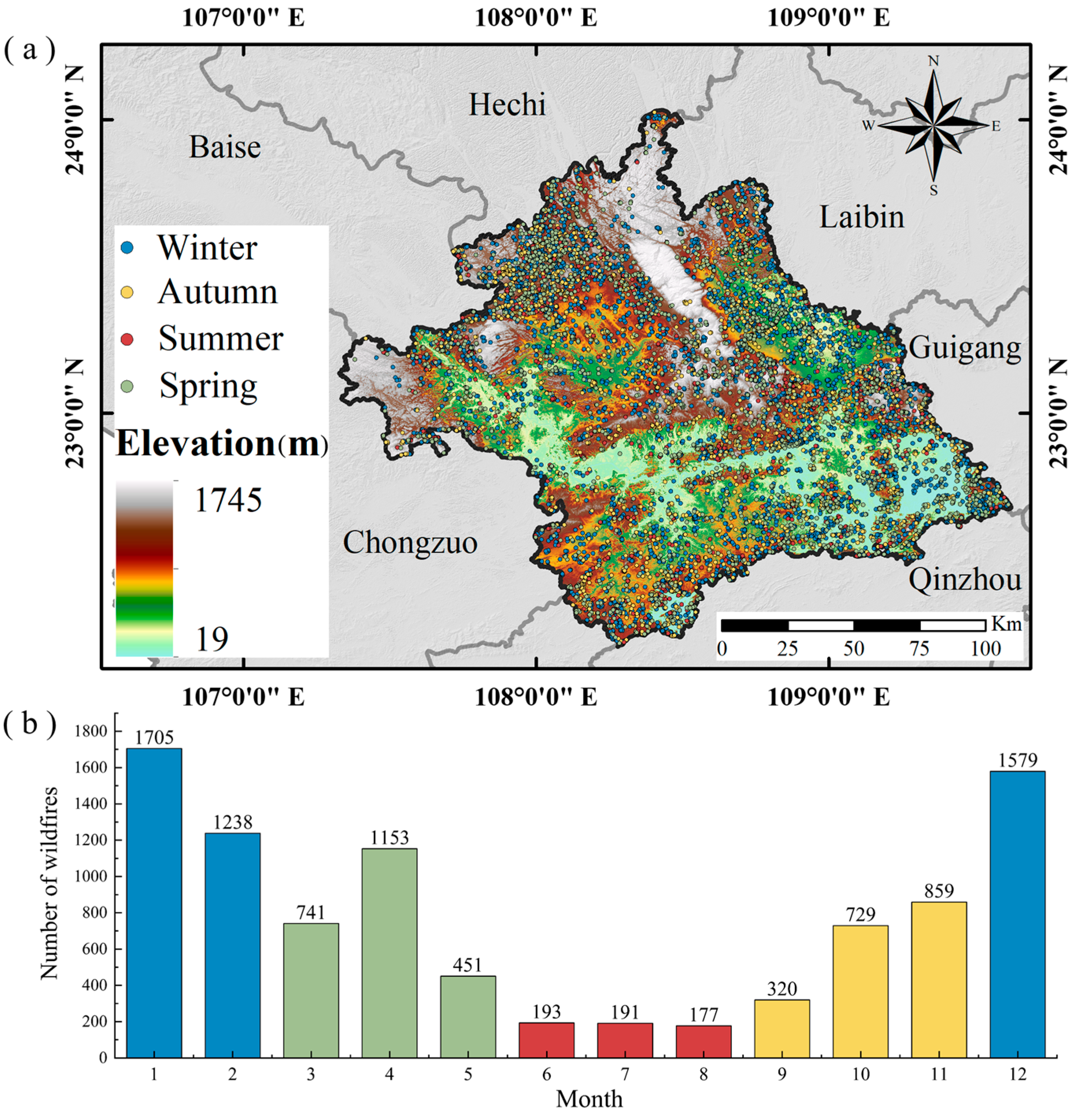
(5) Based on sample density and remote sensing images, eliminating non-target points that represent long-term static thermal anomalies, such as thermal power plants and metallurgical factories. In the end, 9336 wildfire samples were obtained. Among them, the numbers of wildfires in spring (March to May), summer (June to August), autumn (September to November), and winter (December to February) were 2345, 561, 1908, and 4522, respectively. The distribution of wildfire samples in each season within the study area is shown in Figure 1a, while the statistical information of wildfire samples within each season from 2013 to 2022 is presented in Figure 1b. It is evident that the wildfire samples in Nanning are predominantly concentrated in spring and winter, with relatively fewer occurrences in summer and autumn.

2.3. Wildfire Driving Factors

This study selected 15 wildfire driving factors from both seasonal and nonseasonal perspectives. Seasonal factors include the normalized difference vegetation index (NDVI), rainfall, temperature, and wind speed. Non-seasonal factors include 11 factors, including elevation, slope, and population density. The basic information of these factors is presented in

Table 1. Information on wildfire driving factors.

Category	Factors	Source of Data	Format and Scale	Resolution
Seasonal	NDVI	Landsat 8 OLI (2013–2022)	30 m	.tiff
	Rainfall	CHIRPS dataset (2013–2022)	5566 m	.tiff
	Temperature	ERA5-Land Reanalysis Dataset (2013–2022)	11,132 m	.tiff
	Wind speed			.tiff
Nonseasonal	Elevation	SRTM V3_30 m DEM	30 m	.tiff
	Slope			.tiff
	Aspect			.tiff
	Curvature			.tiff
	Topographic wetness index (TWI)			.tiff
	Stream power index (SPI)			.tiff
	Distance to rivers	National Catalogue Service for Geographic Information (in Chinese)	1:250,000 m	.shp
	Distance to roads			.shp
	Population density	WorldPop Dataset	1000 km	.tiff
	Land use	GlobeLand30 V2020 Dataset	30 m	.tiff
	Soil type	Harmonized World Soil Database	5′	.tiff

. To facilitate the analysis, all factor visualization images were projected onto the UTM_Zone_49N coordinate system and resampled to a 30 m × 30 m grid size consistent with the DEM, resulting in a total of 24,566,450 grid cells.

2.3.1. Nonseasonal Factors

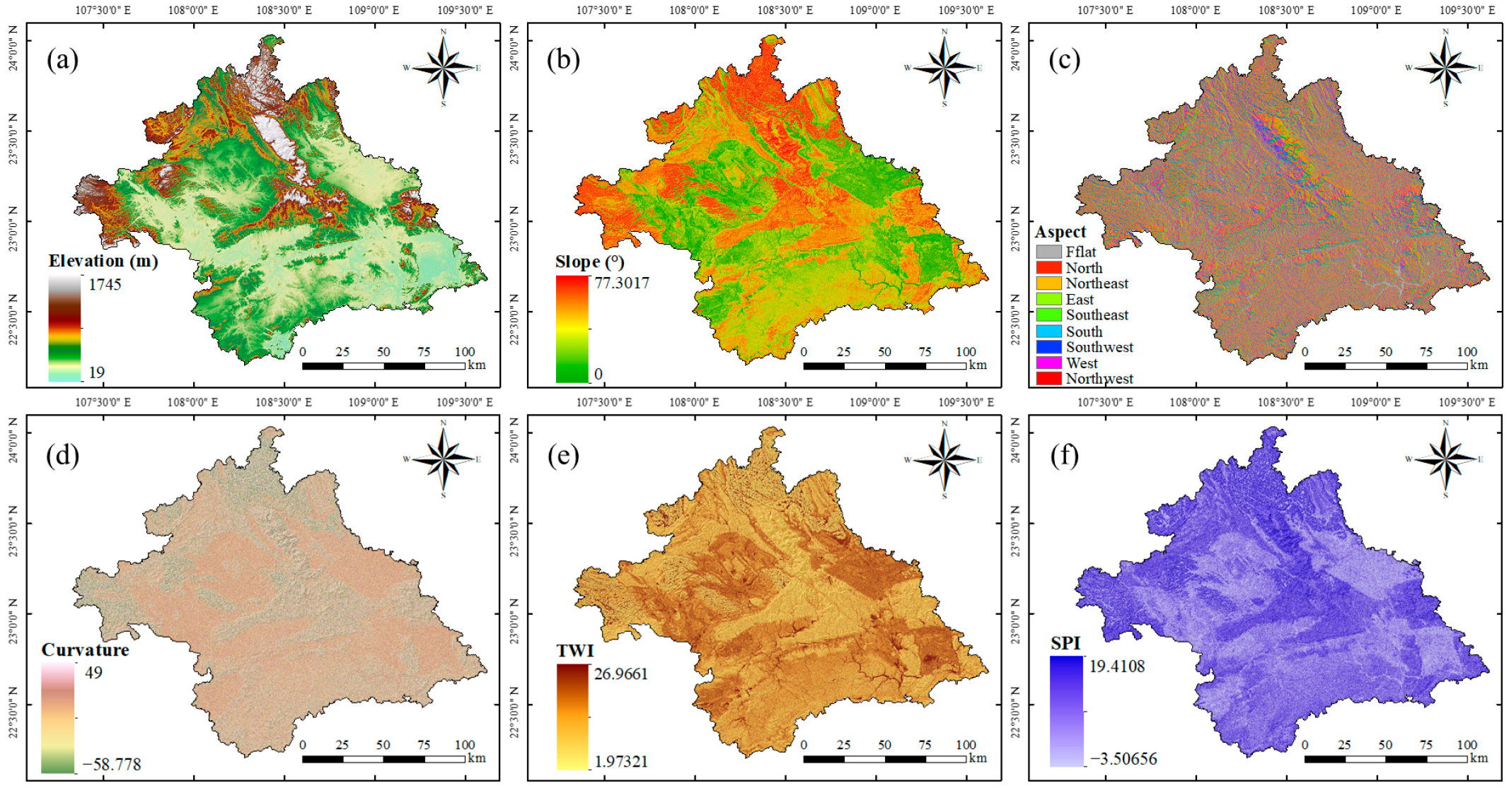
Topographical factors have a significant impact on wildfire occurrence (Figure 2). Elevation influences human activities and vegetation distribution and interacts with local climatic conditions, collectively affecting the initiation and spread of wildfires [56]. Slope plays a crucial role in fire propagation [57]. In general, steeper slopes facilitate the rapid spread of wildfires. Specific aspects can result in varying levels of sunlight exposure, influencing vegetation growth and dryness and thereby affecting wildfire occurrence [58]. Different curvatures can lead to differences in vegetation distribution and moisture, further influencing wildfire incidence [59]. TWI and SPI can reflect surface moisture and water flow energy, respectively, collectively impacting vegetation coverage and the exposure of combustible materials [9]. The formulae for calculating TWI and SPI are as follows.

$$TWI=\mathit{ln}(\alpha /\mathit{tan}\theta )$$

(1)

$$SPI=\mathit{ln}(\alpha \times \mathit{tan}\theta )$$

(2)

where $\alpha$ corresponds to the upstream catchment and $\theta$ represents the inclination angle in radians.

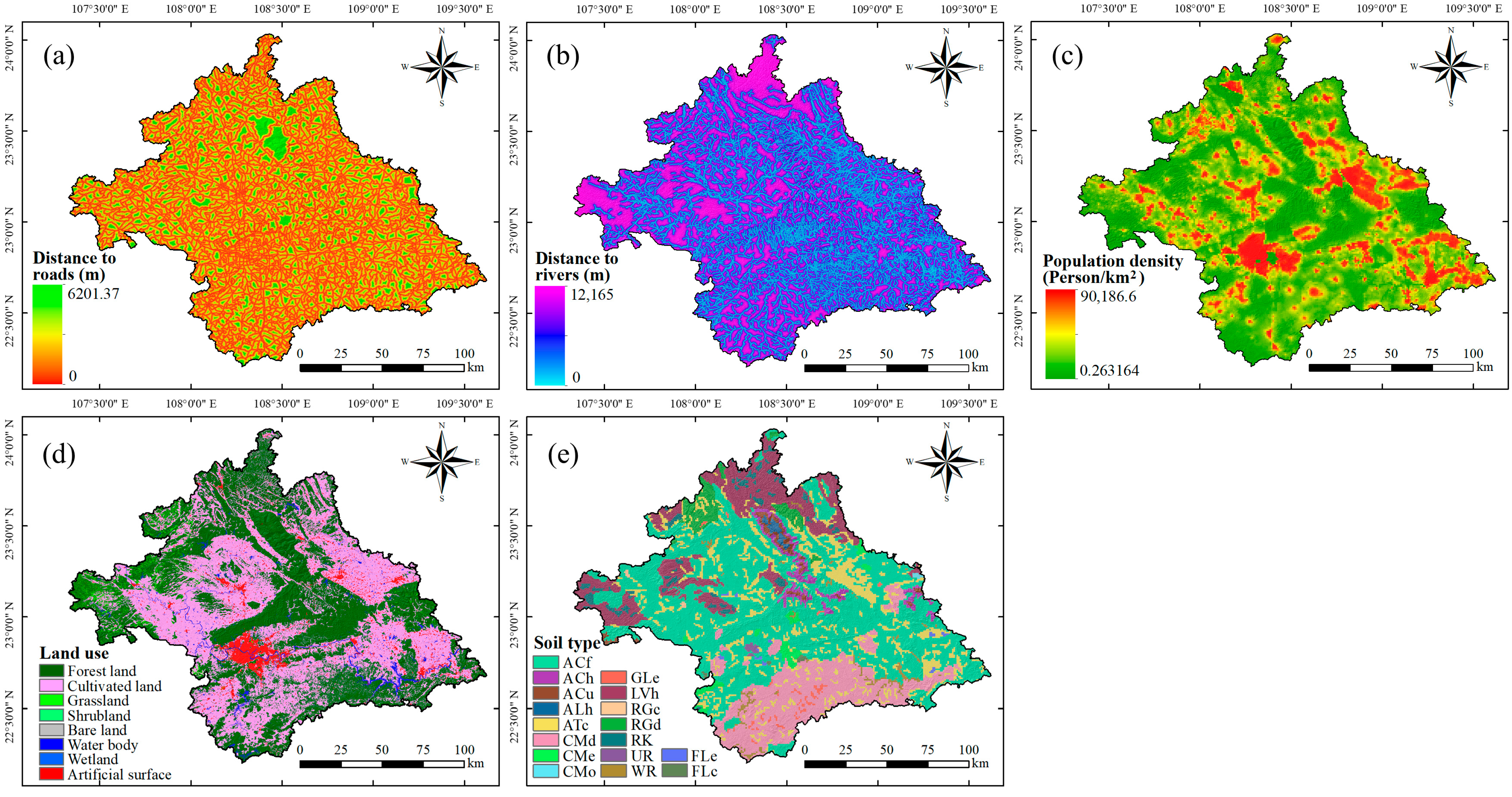
Furthermore, factors such as distance to rivers, distance to roads, population density, land use, and soil type also have an impact on the occurrence and spread of wildfires (Figure 3). Distance to rivers reflects, to some extent, the surface’s moisture level, thereby influencing vegetation growth [60]. Distance to roads and population density jointly indicate human activities, evaluating the extent to which engineering activities and improper use of fire sources contribute to wildfire disasters [18,35]. Land use types have a certain influence on wildfire occurrence. Different land use types provide varying vegetation types and fuel loads, potentially affecting the probability and spread rate of fires [61]. Soil type reflects the composition and characteristics of the soil. Different soil types have varying effects on vegetation growth and water retention. Soil moisture, water storage capacity, and vegetation health are all associated with the occurrence and spread of wildfires [49].

2.3.2. Seasonal Factors

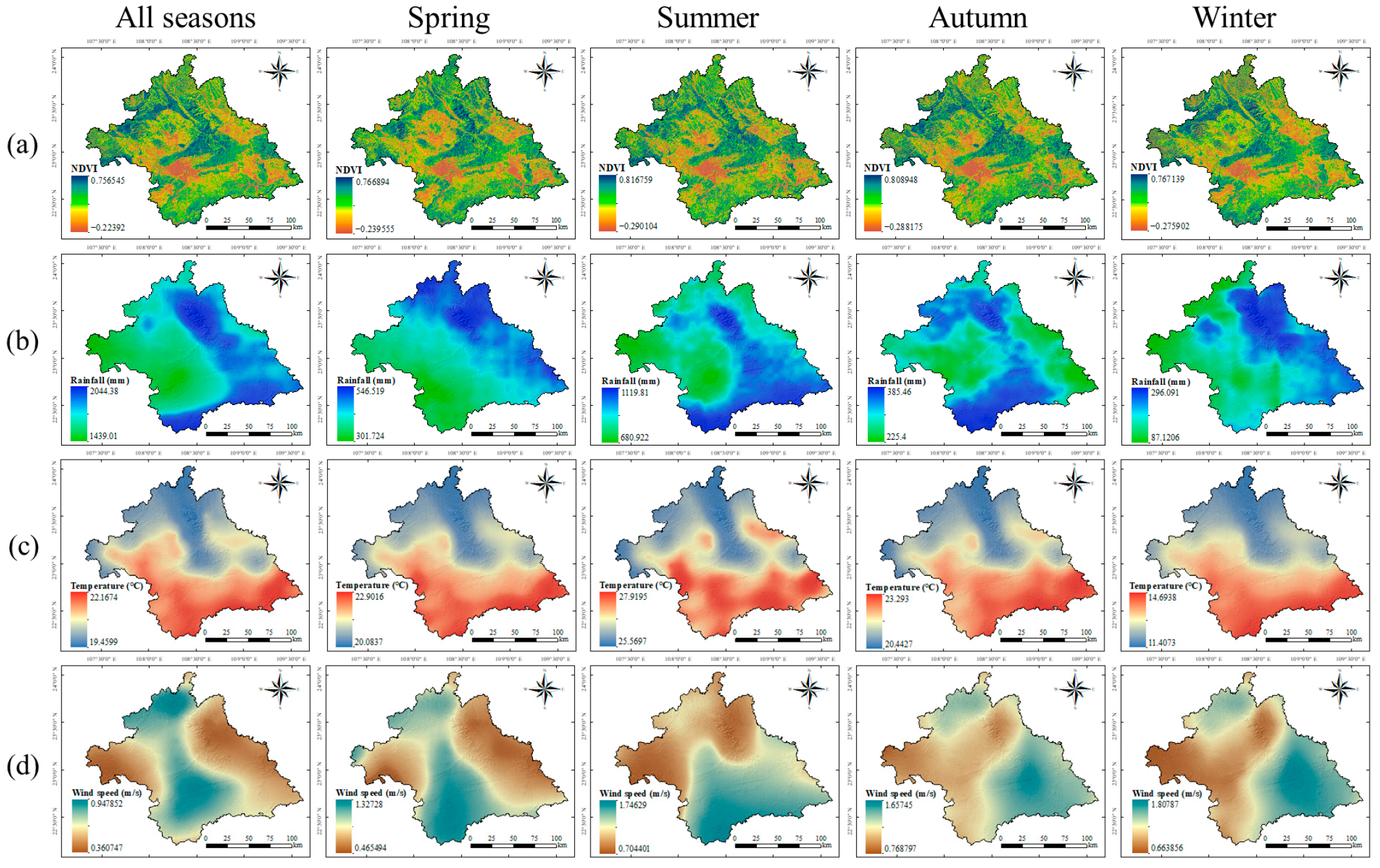
Due to the significant impact of vegetation coverage and climatic conditions on the occurrence and spread of wildfires during different seasons, this study selected seasonal factors from these two aspects. The climatic factors include rainfall, temperature, and wind speed. Rainfall is a crucial climatic factor that determines the water supply for vegetation growth [62]. In Nanning, the highest rainfall occurs during the summer, while the rainfall is relatively lower in spring and autumn, and the lowest in winter. Variations in rainfall directly affect the growth status of vegetation and surface moisture, thereby influencing the probability of wildfire occurrence. Temperature variations affect vegetation growth and dryness, with higher temperatures favoring wildfire occurrence [63]. In Nanning, the highest temperatures are experienced in summer, while the lowest temperatures occur in winter, and spring and autumn temperatures fall between the two extremes. Changes in wind speed impact the spread of fire and the rate of wildfire propagation [64]. In Nanning, the highest wind speeds are observed in winter, while lower wind speeds are recorded in summer and autumn, and the lowest wind speeds occur in spring. Additionally, NDVI, serving as a metric for assessing vegetation condition, reflects the density and health of vegetation. Areas with abundant vegetation coverage are likely to provide a greater fuel load [65]. The calculation formula is shown as Equation (3).

$$NDVI=\frac{NIR-Red}{NIR+Red}$$

(3)

where $Red$ is the red band and $NIR$ is the near-infrared band.

To explore the influence of seasonal differences in terms of the above factors on the assessment of wildfire danger, data collection and processing were conducted for five different periods: all seasons, spring, summer, autumn, and winter, as shown in Figure 4.

2.4. Ecological Vulnerability Factors

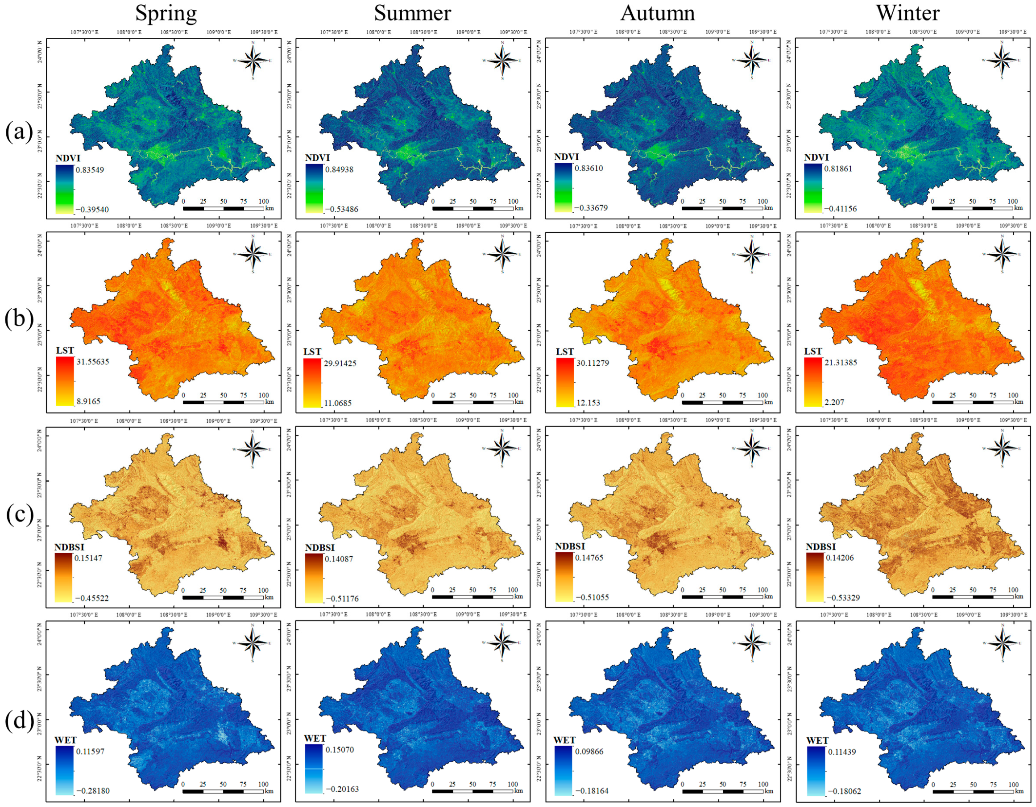
The remote sensing ecological index (RSEI) is an aggregate index that utilizes remote sensing data to swiftly assess the ecological conditions [66]. This approach employs four ecological variables, namely, greenness (representing vegetation), heat (representing temperature), wetness (representing soil moisture), and dryness (representing built areas), to evaluate the ecological status [67]. In general, higher values of greenness and wetness indicate higher vegetation coverage, greater soil and surface vegetation moisture, and a better ecological environment. Conversely, greater values of the heat and dryness indicators indicate higher surface temperatures, intensified soil and built-up areas, and poorer ecological environments [68,69]. By integrating these four indicators, the ecological conditions within the region can be visually depicted [70,71]. In this study, we calculated the four indicators of RSEI using Landsat 8 OLI images. And the RSEI was selected as an evaluation index to measure the ecological condition and vulnerability in different seasons. Specifically:

Greenness is represented by the NDVI. NDVI is a reliable indicator of vegetation dynamics and is widely used to assess vegetation growth conditions [72].

Heat is denoted by land surface temperature (LST) [73]. The calculation is based on Landsat 8 images using the atmospheric correction method, which is given in Equations (4) and (5):

$$LST=\frac{K_2}{\mathit{ln}(\frac{K_1}{B\left(T_s\right)}+1)}$$

(4)

$$B\left(T_s\right)=\frac{L_T-L_{\uparrow }-\beta (1-\theta )L_{\downarrow }}{\beta \theta }$$

(5)

where $K_1$ and $K_2$ are calibration coefficients; $L_T$ represents the land surface temperature in the thermal infrared band of the satellite; and $L_{\uparrow }$ and $L_{\downarrow }$ represent the upwelling and downwelling atmospheric radiance, respectively. $\beta$ denotes the transmissivity of the thermal infrared band, and $\theta$ represents the surface emissivity.

Dryness is represented by the normalized difference built-up and soil index (NDBSI), which is derived from a combination of the index-based built-up index (IBI) and soil index (SI) [74,75]. The mathematical expressions for the calculation are shown in Equations (6)–(8).

$$NDBSI=\frac{IBI+SI}{2}$$

(6)

$$IBI=\frac{\frac{2SWIR1}{SWIR1+NIR}-\left(\frac{NIR}{NIR+Red}+\frac{Green}{Green+SWIR1}\right)}{\frac{2SWIR1}{SWIR1+NIR}+\left(\frac{NIR}{NIR+Red}+\frac{Green}{Green+SWIR1}\right)}$$

(7)

$$SI=\frac{[\left(SWIR1+Red\right)-(NIR+Blue\left)\right]}{[\left(SWIR1+Red\right)+(NIR+Blue\left)\right]}$$

(8)

where $Blue$, $Green$, $Red$, $NIR$, and $SWIR1$ correspond to the spectral bands representing the blue, green, red, near-infrared, and first short-wave infrared bands, respectively.

Wetness is determined using tasseled cap transformation, which effectively reflects the surface humidity status [76]. The calculation formula is shown in Equation (9).

$$\begin{gathered} WET=0.1511\times Blue+0.1973\times Green+0.3283\times Red \\ +0.3404\times NIR-0.7117\times SWIR1+0.4559\times SWIR2 \end{gathered}$$

(9)

where $Blue$, $Green$, $Red$, $NIR$, $SWIR1$, and $SWIR2$ refer to the bands representing the blue, green, red, near-infrared, first short-wave infrared, and second short-wave infrared wavelengths, respectively.

Considering the variable and cloudy weather conditions in Nanning, a single-year and single-season image dataset is insufficient to fully cover the entire study area. Therefore, we utilized a collection of Landsat 8 OLI images from 2018 to 2022 using the Google Earth Engine (GEE) platform. To ensure data quality, we applied image masking to areas with cloud cover exceeding 20% in order to minimize the influence of atmospheric interference. By incorporating images within this temporal framework, we calculated the average values of four indicators for different seasons, aiming to provide a comprehensive representation of the ecological environment. The ecological indicators for each season are shown in Figure 5.

3. Methods

The methodology employed in this research consisted of three stages.

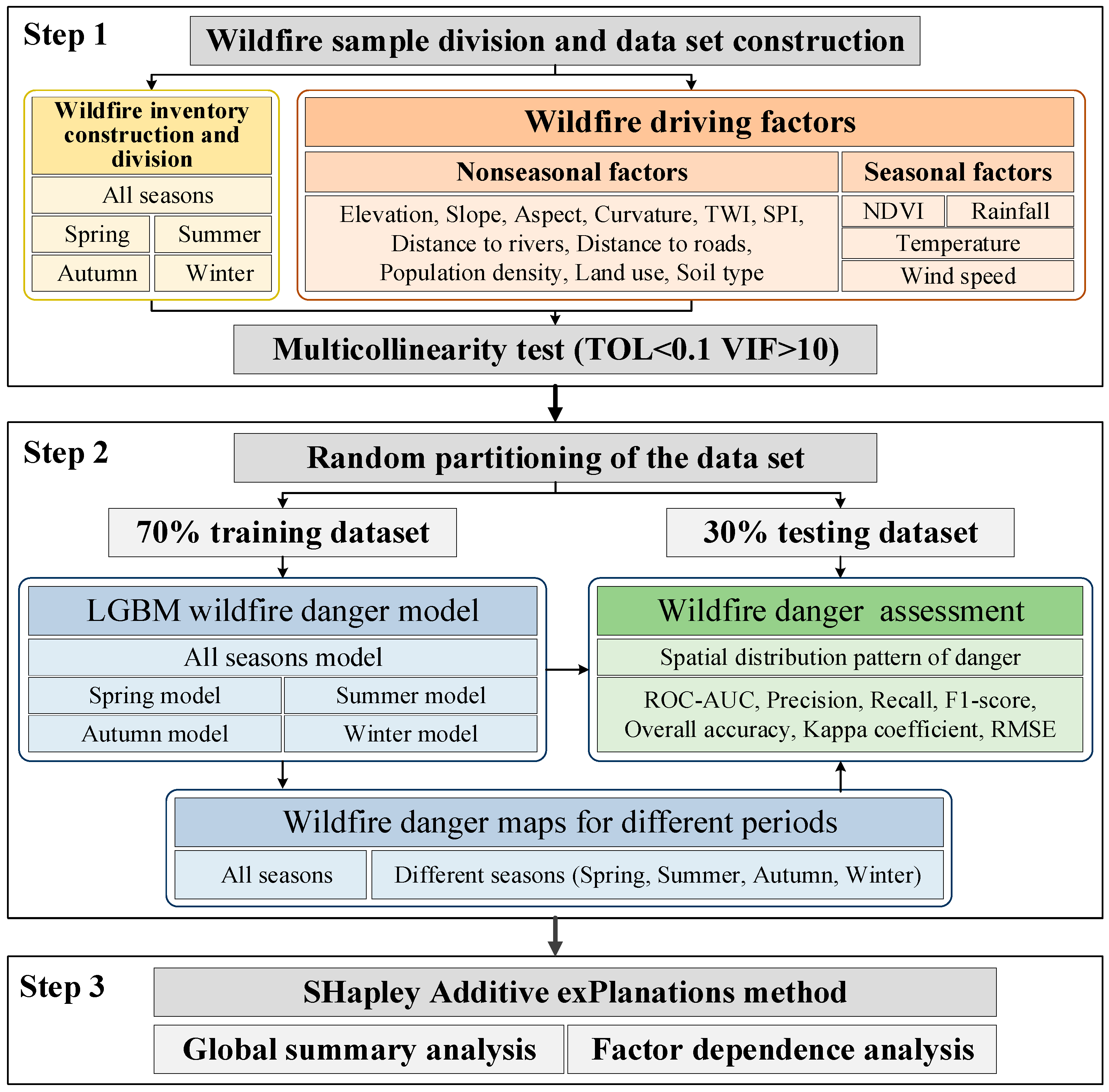
In the first stage, we aimed to construct wildfire danger models for different seasons in Nanning using an ML algorithm. We explored the prediction performance differences of wildfire danger based on annual and quarterly scales, analyzed the spatial distribution characteristics of wildfire danger in different seasons, and assessed the variation in the degree of contribution of each factor on a seasonal scale. The main procedures are described as follows. Initially, we established a spatial database to acquire and categorize wildfire samples from five distinct periods: all seasons, spring, summer, autumn, and winter. Additionally, we gathered wildfire driving factors corresponding to each of these periods. Subsequently, we conducted multicollinearity analysis on the factors for different periods to ensure their independence. Second, we randomly divided the modeling datasets for different periods into training and testing datasets according to a ratio of 7:3. Based on the training set, we used the light gradient boosting machine (LGBM) algorithm to construct wildfire danger models for different periods and generated wildfire danger maps for each season to assess their spatial distribution. Based on the test set, multiple evaluation metrics were used to evaluate the zonal rationality and predictive performance of each model. Third, we employed the SHapley Additive exPlanations (SHAP) method to assess the importance variation in wildfire driving factors across different seasons and focused on analyzing the differences in the influences of seasonal factors on wildfire danger prediction results. The overall technology roadmap is depicted in Figure 6.

In the second stage, a vulnerability assessment of the ecological environment was conducted for different seasons, as shown in Figure 7. Firstly, Landsat imagery data were collected and divided according to the seasons. The greenness, heat, wetness, and dryness indicators were calculated and obtained for each season, and then normalized. Subsequently, principal component analysis (PCA) was applied to integrate the four indicators in order to calculate the remote sensing ecological index (RSEI) for each season. Finally, based on the spatial distribution of the RSEI, the vulnerability of the ecological environment in Nanning was assessed for each season.

In the third stage, the wildfire risk assessment was conducted for different seasons in Nanning. Following the disaster risk assessment method of the United Nations Department of Humanitarian Affairs (UNDHA), the wildfire danger model for each season was integrated with the ecological vulnerability model to construct the wildfire risk model for the corresponding season. Additionally, the spatial distribution characteristics of wildfire risk were summarized for each season, providing a scientific basis for the prevention and management of wildfire disasters in Nanning.

3.1. Wildfire Danger Assessment Method Based on ML Algorithm

3.1.1. Light Gradient Boosting Machine (LGBM)

The light gradient boosting machine (LGBM) is a ML algorithm based on the gradient boosting decision tree (GBDT) [77]. LGBM stands out due to its algorithm based on histograms and a leaf-wise growth strategy, which effectively reduces memory usage and computation time while handling sparse data. Moreover, LGBM incorporates various strategies, such as regularization, to prevent overfitting and supports multi-threading and parallel computing, allowing for efficient processing of massive data and high-dimensional features. As a result, LGBM offers faster processing speed, lower memory consumption, and improved accuracy, making it a valuable tool for wildfire danger assessment [78,79]. LGBM utilizes a gradient-boosting algorithm to enhance model accuracy, and the calculation formula is as follows:

$$y_{pred}=\sum _{i=1}^n(Lr\times f_i(x\left)\right)+y_0$$

(10)

where $y_{pred}$ represents the final predicted value, $\mathrm{L}\mathrm{r}$ denotes the learning rate, $f_i\left(x\right)$ represents the prediction value of the $i$-th decision tree, and $y_0$ is the initial predicted value.

In addition to using wildfire samples as positive samples, ML models also require negative samples to construct the data foundation for the purpose of building the wildfire danger regression prediction model [9]. In this study, equal numbers of negative samples were randomly selected in areas with low historical wildfire density, and the distance between samples was greater than 500 m to ensure the randomness of the negative sample region’s characteristics. Specifically, the numbers of negative samples for spring, summer, autumn, and winter were 2345, 561, 1908, and 4522, respectively. Wildfire-positive samples were assigned a value of “1”, while negative samples were assigned a value of “0”. In total, 70% of the samples were randomly selected as the training set, and the remaining 30% were used as the test set. The training set was used for model training and construction, while the test set was used to verify the predictive performance of the danger models for each period. In this study, we employed the grid search method for hyperparameter tuning to optimize the performance of our danger prediction model. K-fold cross-validation with a value of 10 was used to construct a more reliable and accurate model. The hyperparameter tuning results for the models in each period are shown in

Table 2. Hyperparameter adjustment results.

Hyperparameter	All Seasons	Spring	Summer	Autumn	Winter
max_depth	13	7	7	10	11
num_leaves	80	90	50	50	50
colsample_bytree	0.8	0.5	0.4	0.6	0.7
n_estimators	250	270	250	290	300
min_child_samples	7	6	4	7	4

.

3.1.2. Performance Assessment of Danger Models

This study selected multiple indicators in order to comprehensively evaluate the predictive performance of the wildfire danger models from different dimensions. The receiver operating characteristic (ROC) curve is a common method used to describe the classification performance of the model [80]. The ROC curve plots the true positive rate (TPR) on the vertical axis and the false positive rate (FPR) on the horizontal axis, and the area under the curve (AUC) represents the model’s classification ability. The AUC value ranges from 0.5 to 1, where a value closer to 1 indicates a better classification performance of the model [81]. Precision represents the proportion of correctly predicted wildfire samples among all predicted wildfire samples. It measures the accuracy of positive predictions [82]. Recall measures the proportion of correctly predicted wildfire samples among all actual wildfire samples. It captures the ability of the model to identify positive samples [37]. The F1 score combines both precision and recall into a single metric, allowing for a comprehensive evaluation of the model’s effectiveness in predicting wildfires [83]. Overall accuracy (OA) refers to the proportion of correctly predicted samples to the total number of samples [84]. The kappa coefficient (KC) is a statistical measure used to assess the consistency between the model’s predicted results and the true labels. A value closer to 1 indicates a higher level of agreement between the model’s predictions and the true labels [34]. The root mean squared error (RMSE) is used to measure the average difference between the model’s predicted values and the true labels. A smaller RMSE indicates a smaller error between the model’s predicted results and the true values, indicating a better predictive capability of the model [18]. The above indicators are calculated as follows:

$$AUC=\frac{1}{2}\times (\frac{TP}{TP+FN}+\frac{TN}{TN+FP})$$

(11)

$$Precision=\frac{TP}{TP+FP}$$

(12)

$$Recall=\frac{TP}{TP+FN}$$

(13)

$$F1score=\frac{2\times Precision\times Recall}{Precision+Recall}$$

(14)

$$OA=\frac{TP+TN}{TP+FN+TN+FP}$$

(15)

$$KC=\frac{OA-P_e}{1-P_e}(P_e=\frac{(TP+FN)(TP+FP)(TN+FN)(FP+TN)}{{(TP+FN+FP+TN)}^2})$$

(16)

$$RMSE=\sqrt{\frac{1}{n}{\sum }_{i=1}^n{(Y_{pre\_i}-Y_i)}^2}$$

(17)

In Equations (2)–(5), $TP$ (true positive) indicates the number of wildfire samples that were correctly classified as wildfire. $TN$ (true negative) indicates the number of non-wildfire samples that were correctly classified as non-wildfire. On the other hand, $FP$ (false positive) is the number of non-wildfire samples that were incorrectly classified as wildfire. $FN$ (false negative) is the number of wildfire samples that were incorrectly classified as non-wildfire. In Equation (6), $n$ represents the number of samples. $Y_{pre\_i}$ and $Y_i,$ respectively, represent the predicted value and the actual value of the $i$-th sample.

3.1.3. SHapley Additive exPlanations (SHAP) Method

SHapley Additive exPlanations (SHAP) is an interpretable method based on game theory which is used to explain the outputs of any ML model [85]. Its essence lies in the Shapley value, which is a method of allocating contributions to total consumption based on players’ participation. The interpretability of Shapley values is manifested as an additive feature attribution method, where the model’s predictions are explained as the sum of attribution values for each input feature [49,86]. We employed the Tree-SHAP method, which considers tree-based models in conjunction with an input dataset X of size N × M, generating an N × M matrix with Shapley values (where N represents the number of samples and M denotes the number of features), enabling the comprehensive global explanation of wildfire danger models constructed at different time periods. The calculation formula for Shapley is as follows:

$${\varphi }_j(x_i)=\sum _{S\subseteq N/\left\{j\right\}}\frac{M!\times \left(\left|S\right|\right)\times \left(M-\left|S\right|-1\right)!}{M!}[f_{S\bigcup \left\{j\right\}}\left(x_i\right)-f_S\left(x_i\right)]$$

(18)

where $x_i$ represents the $i$-th sample; $j$ denotes one of the features; $S$ represents a feature subset that does not include the feature $j$; $f_S\left(x_i\right)$ represents the model’s prediction output when the feature subset $S$ is removed from the model; $f_{S\bigcup \left\{j\right\}}\left(x_i\right)$ represents the model’s prediction output when the feature $j$ is added to the feature subset $S$; and $M$ is the total number of samples in the dataset. In this study, we utilized the SHAP method to generate global summary plots and single dependence plots. These plots were used to analyze the direction and contribution of each factor in predicting wildfire danger during different periods. The dependence relationship between the attribute values of seasonal factors and the prediction results of danger was evaluated.

3.2. Ecological Vulnerability Assessment Method Based on RSEI

Disaster vulnerability can be defined as the degree of vulnerability to damage that an area or system exhibits in the face of a disaster [87]. It reflects the resistance and recovery capacity of the subject under disaster conditions. Specifically in the context of the ecological environment, disaster vulnerability refers to the vulnerability of various components in the ecosystem (such as vegetation, soil, water resources, etc.) to disasters. It takes into account the responsiveness of the ecosystem’s structure, functions, and dynamic processes to disasters. In this study, we used RSEI to assess the vulnerability of wildfire disasters in different seasons by integrating greenness, heat, wetness, and dryness in the study area.

In order to mitigate the influence of varying scales and dimensions among different indicators on the evaluation results, normalization was applied to the indicators [73]. The normalization process is represented by Equation (19).

$${NI}_i=\frac{I_i-I_{min}}{I_{max}-I_{min}}$$

(19)

where ${NI}_i$ represents the normalized value of each indicator, $I_i$ represents the value of each indicator at the $i$-th pixel, and $I_{min}$ and $I_{max}$ represent the minimum and maximum values of each indicator, respectively.

Subsequently, the principal component analysis (PCA) method was employed to objectively allocate weights based on the contribution rates of NDVI, LST, WET, and NDBSI. This approach helps to reduce biases caused by subjective weighting based on personal experience [88,89]. The final outcome is a composite index, RSEI, which is used to assess the ecological environment status [90]. The calculation formulas are presented as Equations (20) and (21).

$${RSEI}_0=\left\{PCA\left[f(NDVI,LST,NDBSI,WET)\right]\right\}$$

(20)

$$RSEI=\frac{{RSEI}_0-{RSEI}_{0_{min}}}{{RSEI}_{0_{max}}-{RSEI}_{0_{min}}}$$

(21)

where ${RSEI}_0$ denotes the initial remote sensing ecological index obtained through PCA; ${RSEI}_{0_{min}}$ is the minimum value of ${RSEI}_0$; ${RSEI}_{0_{max}}$ is the maximum value of ${RSEI}_0$; and $RSEI$ signifies the standardized remote sensing ecological index, ranging from 0.0 to 1.0. A higher RSEI value indicates a better ecological environment status, and it also suggests that the occurrence of wildfire may result in more severe ecological damage. Conversely, a lower RSEI value suggests that the ecological environment is relatively less susceptible to the impacts and damage caused by wildfires.

3.3. Wildfire Risk Assessment Method

The natural disaster risk arises from the interaction between disaster danger and vulnerability. It represents the potential risk of losses to specific entities resulting from the occurrence of the disaster [91,92,93]. The assessment of disaster risk combines both these factors and quantifies the level of risk by evaluating potential impacts and losses [94,95]. The calculation formula for disaster risk is shown in Equation (22).

$${Risk}_i={Danger}_i\times {Vulnerability}_i$$

(22)

where ${Danger}_i$ represents the wildfire danger value of the $i$-th pixel, and ${Vulnerability}_i$ represents the ecological vulnerability value of the $i$-th pixel. The resulting ${Risk}_i$ represents the risk of wildfire-induced ecological damage for the $i$-th pixel, ranging from 0 to 1.

4. Results

4.1. Wildfire Danger Assessment

4.1.1. Multicollinearity Test Results

In this study, the multicollinearity between wildfire occurrences and driving factors in different periods was assessed using the SPSS 26.0 data analysis software, as shown in

Table 3. Analysis of the multicollinearity between wildfire driving factors.

Wildfire Driving Factor	All Seasons		Spring		Summer		Autumn		Winter
	TOL	VIF	TOL	VIF	TOL	VIF	TOL	VIF	TOL	VIF
Elevation	0.362	2.766	0.313	3.193	0.283	3.527	0.332	3.011	0.344	2.909
Slope	0.367	2.726	0.339	2.952	0.362	2.763	0.370	2.705	0.358	2.795
Aspect	0.989	1.011	0.993	1.007	0.985	1.015	0.996	1.004	0.997	1.003
Curvature	0.904	1.106	0.908	1.102	0.893	1.120	0.918	1.090	0.919	1.088
TWI	0.559	1.788	0.593	1.686	0.549	1.821	0.562	1.780	0.579	1.726
SPI	0.639	1.566	0.672	1.487	0.645	1.550	0.643	1.555	0.645	1.549
Distance to rivers	0.699	1.430	0.591	1.693	0.624	1.602	0.672	1.489	0.593	1.685
Distance to roads	0.816	1.226	0.691	1.446	0.819	1.220	0.813	1.229	0.773	1.293
Population density	0.911	1.098	0.865	1.156	0.814	1.228	0.833	1.200	0.871	1.148
Land use	0.691	1.448	0.780	1.282	0.669	1.495	0.741	1.349	0.868	1.152
Soil type	0.758	1.320	0.666	1.501	0.724	1.382	0.732	1.367	0.708	1.412
NDVI	0.545	1.833	0.589	1.698	0.510	1.963	0.609	1.642	0.686	1.457
Rainfall	0.802	1.247	0.427	2.340	0.644	1.553	0.813	1.231	0.652	1.533
Temperature	0.467	2.141	0.256	3.909	0.235	4.258	0.367	2.729	0.463	2.158
Wind speed	0.929	1.077	0.726	1.377	0.521	1.919	0.902	1.109	0.865	1.156

. The tolerance (TOL) values for the 15 wildfire-regulating factors in different periods were all above 0.2, and the variance inflation factor (VIF) values were all below 5.0. Among them, elevation had the lowest TOL values and the highest VIF values across all periods. The results indicate that there is no multicollinearity among the factors within each period and no strong mutual influence, ensuring the reliability and effectiveness of the wildfire danger model.

4.1.2. Wildfire Danger Map

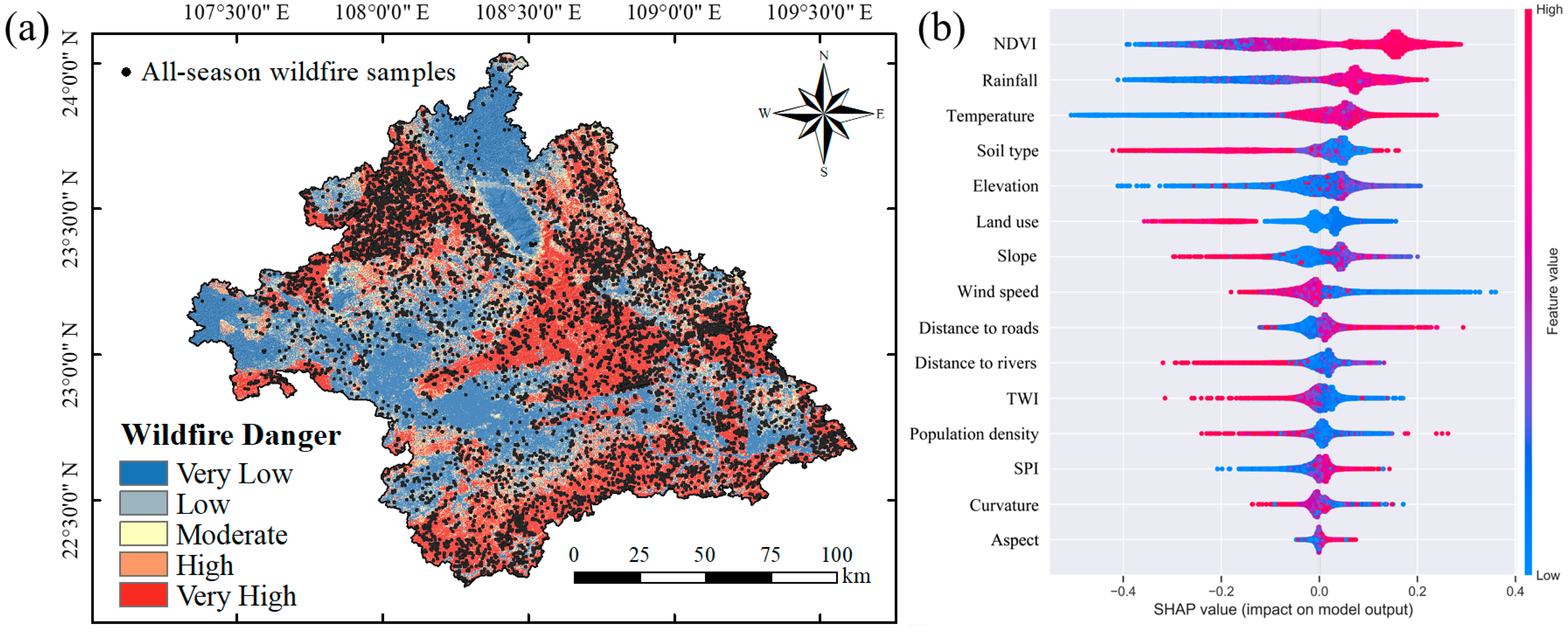
This study initially analyzed the wildfire danger based on all seasons, aiming to identify and understand the influence of seasonal factors and providing the reference for subsequent wildfire danger analyses in different seasons. We classified the regional wildfire danger predictions based on all seasons into five levels: very low, low, moderate, high, and very high, using the classification criteria of [0, 0.2], (0.2, 0.4], (0.4, 0.6], (0.6, 0.8], and (0.8, 1.0], as shown in Figure 8a. It can be seen that areas with high wildfire danger are primarily distributed in the northwest, central-eastern, and southern parts of Nanning, while low danger areas can be found in the northern, western, and southwestern regions of Nanning.

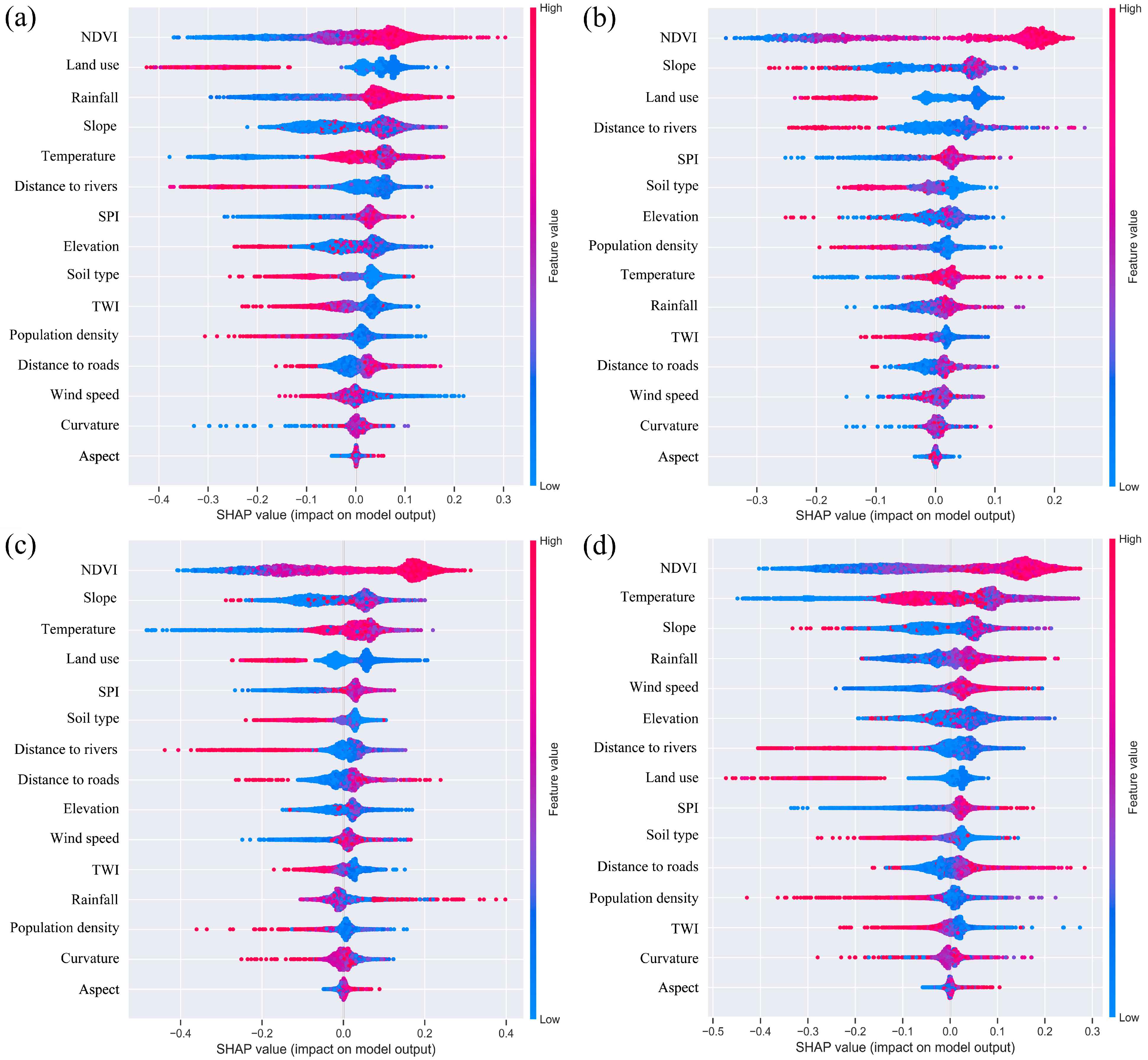
The global interpretation results of the wildfire driving factors are presented in Figure 8b. The SHAP summary plot presents the relationship between model predictions and different factors, as well as the extent of the influence these factors have on the predictions. Each point in the summary plot represents a data sample, with the color indicating the magnitude of the corresponding factor value, where red represents a high value and blue represents a low value. The horizontal axis represents the Shapley values of the sample points, while the vertical axis arranges the factors in descending order of their contributions. The results reveal that the seasonal factors exhibited the most significant impact on wildfire danger in Nanning, with the factor importance rankings for NDVI, rainfall, temperature, and wind speed being 1, 2, 3, and 8, respectively. It is evident that the occurrence of wildfires in Nanning is greatly influenced by seasonal factors.

In order to ensure the comparability of wildfire danger zoning results across different seasons and to establish a consistent probability range for the same danger level across different models, we employed the same zoning interval to classify the danger prediction results for different seasons. The danger zoning results are shown in Figure 9, demonstrating similar spatial distribution patterns of wildfire danger across all seasons as well as during the individual seasons of spring, summer, autumn, and winter. However, the danger zoning results based on different seasons revealed more detailed information, with a higher number of wildfire samples falling within the high-danger zones. Consequently, this approach provides a more comprehensive depiction of the spatial distribution of wildfire danger within different seasons.

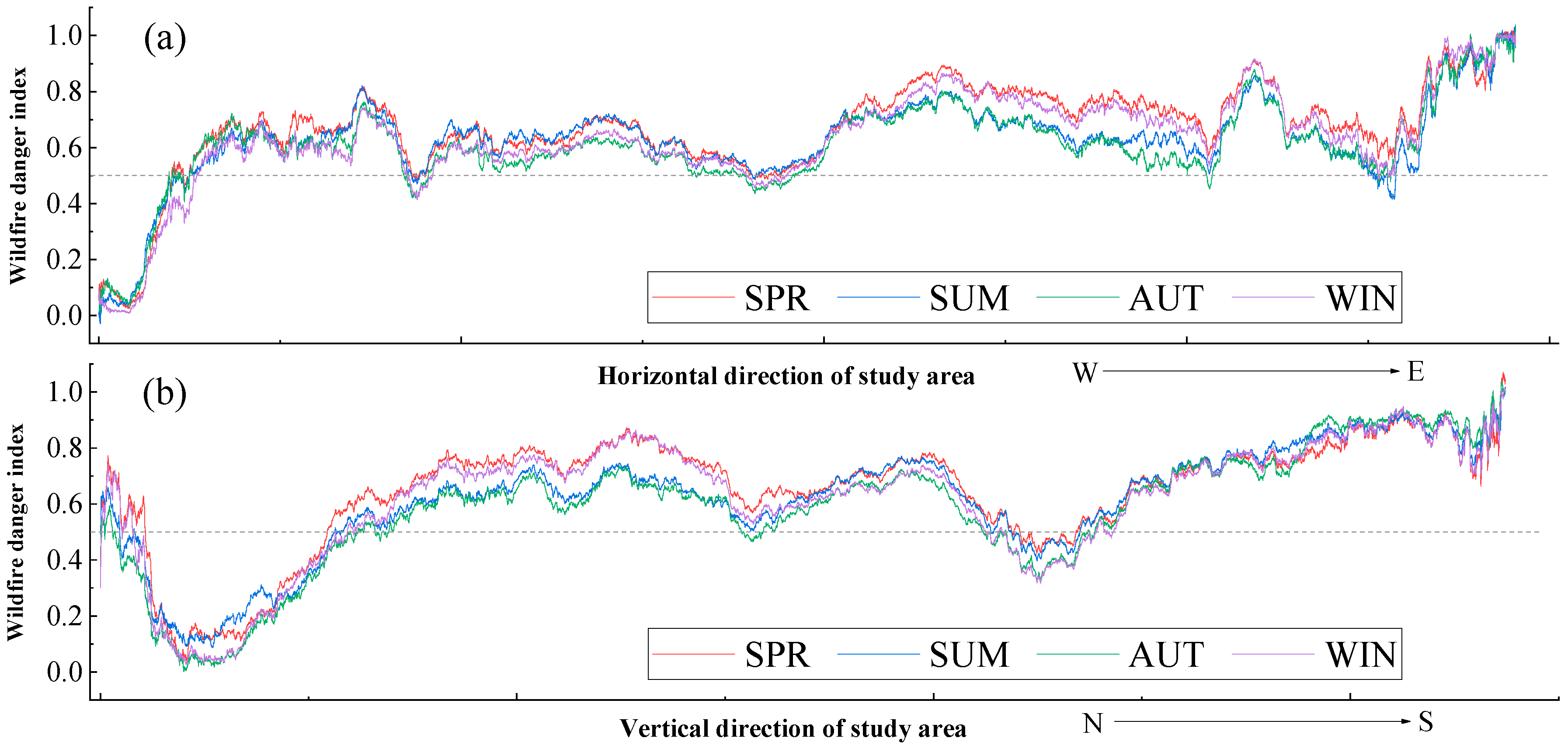
As shown in Figure 10, the wildfire danger in different seasons exhibited a similar trend in the same direction (either horizontally or vertically), with fewer regions having a wildfire danger probability below 0.5. However, there were slight differences in the details, with the danger probabilities in spring and winter being higher in the eastern and northern-central parts of the study area compared to summer and autumn. Additionally, the danger probabilities in the northwestern and southern-central parts of the study area were slightly higher in spring and summer than in autumn and winter.

The detailed statistical information on wildfire danger zoning in different periods is presented in

Table 4. Statistics of wildfire danger zoning results in different periods.

Period	Danger Level	Percentage of Area (P(S)/%)	Proportion of Wildfire Samples (P(N)/%)	Frequency Ratio (P(N)/P(S))
Spring	Very low	16.525	2.263	0.137
	Low	9.619	2.970	0.309
	Moderate	9.687	4.809	0.496
	High	11.889	8.062	0.678
	Very high	52.280	81.895	1.566
Summer	Very low	16.175	1.695	0.105
	Low	12.011	1.695	0.141
	Moderate	12.972	3.955	0.305
	High	14.290	5.650	0.395
	Very high	44.553	87.005	1.953
Autumn	Very low	28.811	3.633	0.126
	Low	11.239	2.768	0.246
	Moderate	9.969	6.574	0.660
	High	12.323	9.516	0.772
	Very high	37.660	77.509	2.058
Winter	Very low	21.615	3.835	0.177
	Low	9.703	4.572	0.471
	Moderate	8.804	6.490	0.737
	High	9.754	9.071	0.930
	Very high	50.125	76.032	1.517
All seasons	Very low	28.130	4.833	0.172
	Low	12.185	5.414	0.444
	Moderate	8.838	6.032	0.682
	High	9.107	9.702	1.065
	Very high	41.740	74.019	1.773

. The proportions of very high-danger areas for spring, summer, autumn, winter, and all seasons were 52.28%, 44.553%, 37.66%, 50.125%, and 41.74%, respectively. Among them, summer and autumn had smaller areas of very high danger, while spring and winter had larger areas. The proportions of wildfire samples within the very high-danger areas for spring, summer, autumn, winter, and all seasons were 81.895%, 87.06%, 77.509%, 76.032%, and 74.019%, respectively, while the proportions of wildfire samples within the very low-danger areas were 2.263%, 1.695%, 3.633%, 3.835%, and 4.833%. It can be observed that wildfire danger zoning based on individual seasons can provide a more comprehensive identification of high-danger areas. Compared to the model based on all seasons, this demonstrates better classification performance.

Based on the area of specific danger levels and the number of wildfire samples they contained, we calculated the frequency ratios of different wildfire danger levels in each period. It can be observed that the frequency ratio increased with the increase in wildfire danger level across different periods. And the frequency ratio for the very high-danger areas was greater than 1.0, indicating the rationality of the zoning results in each period. Among them, the summer and autumn exhibited higher frequency ratios for the very high-danger areas compared to all seasons, indicating a better fit with the wildfire samples. On the other hand, the spring and winter showed lower frequency ratios for the very high-danger areas compared to all seasons, indicating a relatively poorer fit with the wildfire samples.

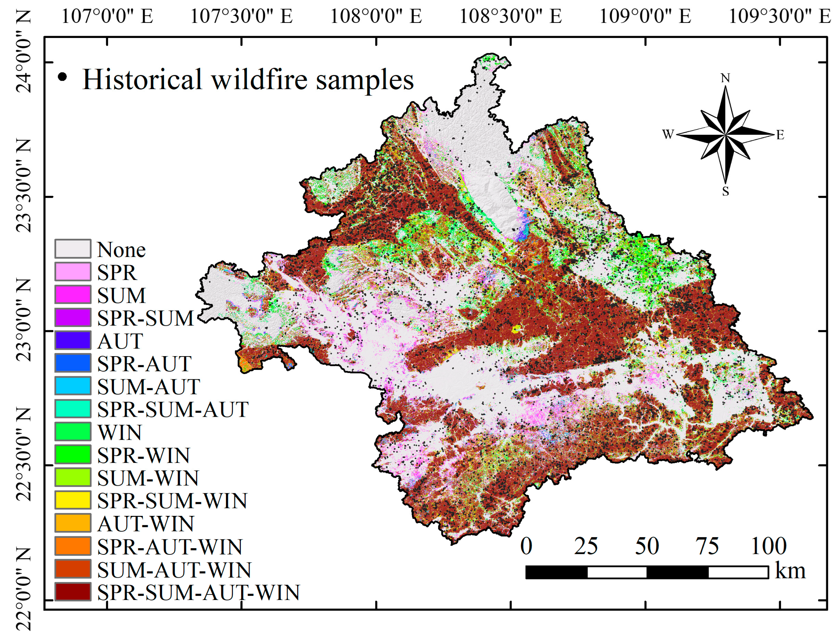
This study employed statistical and computational tools within GIS to analyze the distribution of very high-wildfire-danger areas across different seasons. The seasonal distribution of these areas is depicted in Figure 11, while the statistical results of their respective proportions are presented in

Table 5. Statistical results of very high-wildfire-danger areas by season. SPR: spring; SUM: summer; AUT: autumn; WIN: winter.

Partition Results	Number of Grids/Unit	Percentage of Area/%	Partition Results	Number of Grids/Unit	Percentage of Area/%
None	9,915,568	40.362	WIN	675,323	2.749
SPR	1,005,981	4.095	SPR-WIN	1,260,502	5.131
SUM	542,557	2.209	SUM-WIN	235,855	0.960
SPR-SUM	371,360	1.512	SPR-SUM-WIN	1,307,684	5.323
AUT	73,525	0.299	AUT-WIN	71,726	0.292
SPR-AUT	88,214	0.359	SPR-AUT-WIN	530,584	2.160
SUM-AUT	64,000	0.261	SUM-AUT-WIN	144,539	0.588
SPR-SUM-AUT	191,421	0.779	SPR-SUM-AUT-WIN	8,087,611	32.921

. The results indicate that the proportion of regions prone to wildfire occurrence throughout each season in Nanning was 32.921%. Specifically, during the spring–summer–winter, the spring–winter, and the spring, the proportions of areas susceptible to wildfire were 5.323%, 5.131%, and 4.095%, respectively. It is evident that the seasonal wildfire danger in Nanning is primarily influenced by the spring and winter. It is recommended to implement preventive and control measures in the corresponding areas indicated in Figure 11 during these seasons to enhance the effectiveness of fire prevention efforts.

4.1.3. Model Performance Assessment

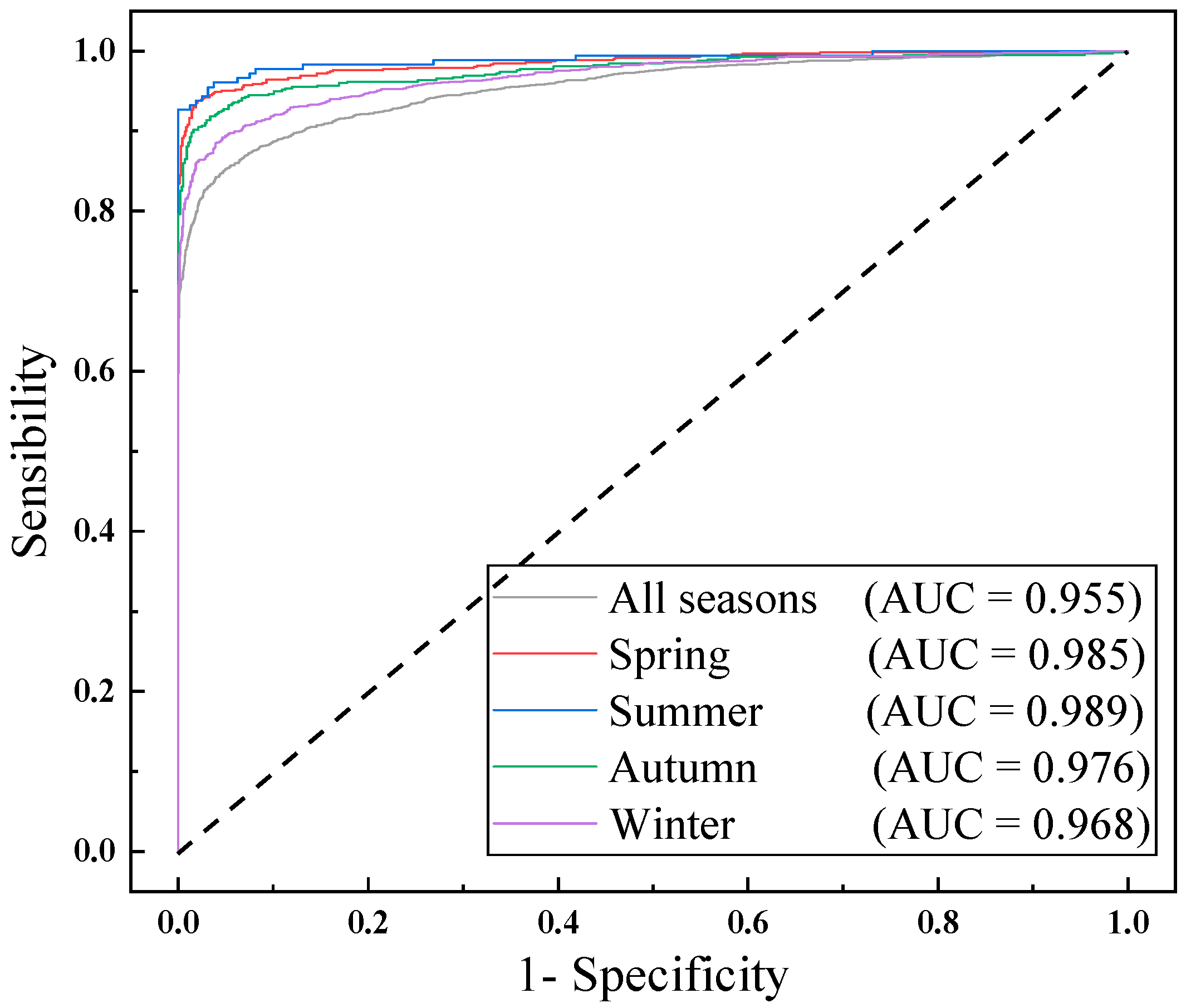
The ROC curves and AUC values were utilized to evaluate the classification performance of the wildfire danger models across different periods, considering the presence and absence of wildfires as two categories. A higher AUC value indicates a stronger classification ability of the model in terms of distinguishing between the presence and absence of wildfires. As shown in Figure 12, the ROC-AUC values for each period, ranked from highest to lowest, are as follows: summer (0.989) > spring (0.958) > autumn (0.976) > winter (0.968) > all seasons combined (0.955). It can be observed that the wildfire danger models constructed based on individual seasons achieved higher ROC-AUC values, indicating superior predictive performance.

The predictive accuracy of wildfire danger models during different time periods is presented in

Table 6. Predictive performance of wildfire danger models of different periods. OA: overall accuracy; KC: kappa coefficient.

Period	Precision	Recall	F1 Score	OA	KC	RMSE
Spring	0.982	0.929	0.955	0.956	0.912	0.209
Summer	0.971	0.944	0.957	0.955	0.911	0.194
Autumn	0.972	0.907	0.938	0.940	0.880	0.234
Winter	0.952	0.888	0.919	0.922	0.843	0.255
All seasons	0.924	0.869	0.895	0.900	0.800	0.279

. The precision of the models during different time periods, ranked in descending order, were as follows: spring (0.982) > autumn (0.972) > summer (0.971) > winter (0.952) > (0.924). The recalls, ranked in descending order, were as follows: summer (0.944) > spring (0.930) > autumn (0.907) > winter (0.888) > all seasons (0.869). The F1 scores, ranked in descending order, were as follows: summer (0.957) > spring (0.955) > autumn (0.938) > winter (0.919) > all seasons (0.985). The results indicate that the wildfire danger models based on individual seasons exhibited a stronger ability to accurately predict and capture wildfires in their respective seasons. The overall accuracies and kappa coefficients of different models, ranked in descending order, were as follows: spring > summer > autumn > winter > all seasons. The RMSE values, ranked in ascending order, were as follows: summer (0.194) < spring (0.209) < autumn (0.234) < winter (0.255) < all seasons (0.279). It can be observed that the wildfire danger model constructed based on all seasons had a relatively weaker ability to distinguish between wildfires and non-wildfires, resulting in a lower level of concordance between predictions and actual observations. Conversely, the models based on individual seasons demonstrated a stronger capability to differentiate between wildfire and non-wildfire areas, resulting in a higher level of consistency between predictions and actual occurrences and a lower level of uncertainty or variability in the model predictions. Additionally, in terms of wildfire prediction performance across different seasons, the performance was better in spring and summer compared to autumn and winter.

In conclusion, due to the close relationship between wildfire occurrence and factors such as climate and vegetation growth, the impact of seasonal factors on wildfires cannot be overlooked in wildfire danger research. Therefore, by constructing wildfire danger models for different seasons, the prediction results can be more targeted, effectively improving the accuracy and reliability of wildfire predictions. In contrast, the assessment of wildfire danger based on all seasons may not comprehensively consider the seasonal differences in climate and vegetation factors, leading to a potential decrease in prediction accuracy. In summary, wildfire danger models based on individual seasons demonstrate superior performance and reliability.

4.1.4. Assessment of Seasonal Differences in the Importance of Factors

Figure 13 displays the summary plots for the wildfire prediction factors in different seasons. It was determined that the importance of factors exhibited both uniformity and difference among different seasons. The uniformity manifested in the consistent prominence of NDVI as the most influential factor in the wildfire danger models across all seasons, displaying a positive correlation with wildfire occurrence. This relationship can be attributed to densely vegetated regions accumulating a greater biomass, thereby increasing the availability of combustible materials. Furthermore, when wildfires transpire, densely vegetated areas often prove challenging to control, resulting in regions with higher NDVI values being more susceptible to such incidents. As for nonseasonal factors, slope emerged as the highest-ranking contributor in terms of importance, exerting a significant influence on wildfire occurrence throughout different seasons. In comparison to other factors, TWI, curvature, and aspect made relatively smaller contributions to the prediction of wildfire danger in each season.

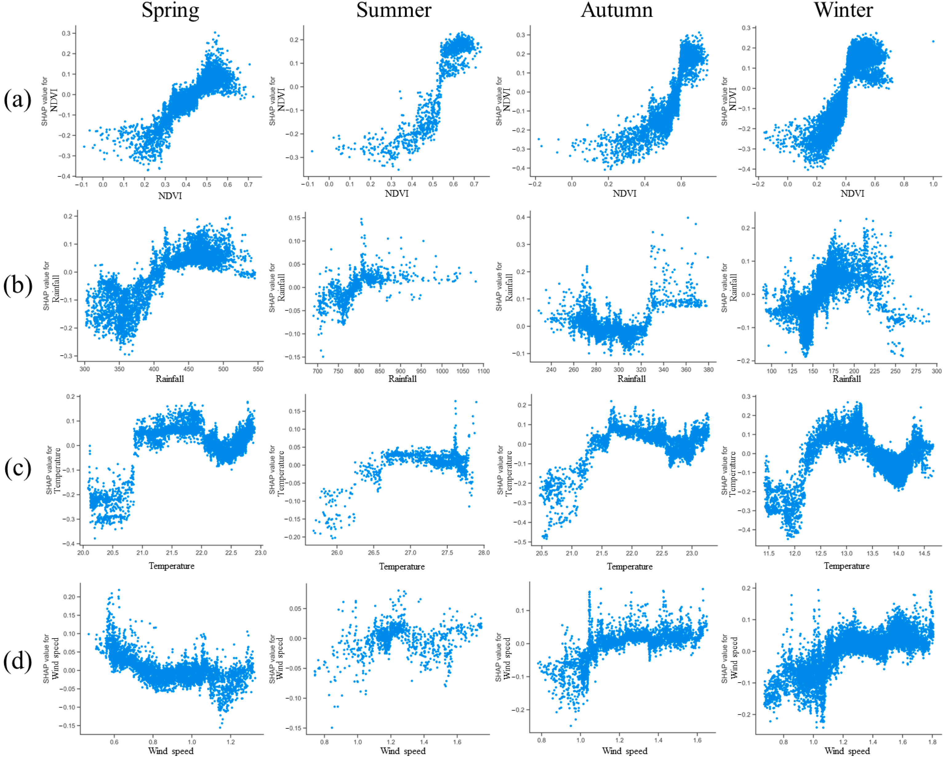
The single dependence plot illustrates the influence of specific attribute values of a factor on the prediction results. As shown in Figure 14 for seasonal factors, the horizontal axis represents the range of factor values, while the vertical axis represents the Shapley values. Each point in the plot represents the degree of impact of a specific attribute value of the factor on the prediction. Generally, when the Shapley value of a sample is greater than 0, it indicates that the specific attribute value of that factor contributes to an increased likelihood of wildfire occurrence. By observing the dependence plots, we can gain insights into how changes in factor values affect the predictions, thereby understanding the model’s dependence on the factors and the stability of the predictions. Combining the analysis with the summary plots revealed that each factor exhibited varying degrees of influence on the prediction of wildfire danger in different seasons. Specifically:

(1)

Spring: NDVI, land use, rainfall, slope, and temperature were the main factors influencing the occurrence of wildfire disasters. Concerning seasonal factors, spring experienced lower rainfall (300–500 mm) and higher temperatures (20.1–22.9 °C). The limited precipitation and warm weather facilitated the growth of vegetation. Additionally, abundant sunshine and dry ground conditions were conducive to the occurrence of wildfires. Spring recorded the lowest wind speeds (0.46–1.33 m/s), which exhibited a negative correlation with wildfire incidence, making a smaller contribution.

(2)

Summer: NDVI, slope, land use, distance to rivers, and SPI played a significant role in the occurrence of wildfire disasters. Regarding seasonal factors, summer had the highest rainfall (700–1100 mm) and the highest temperatures (25.6–27.8 °C). The combination of rainfall and evaporation resulted in increased humidity in the surface and air, thereby suppressing the risk of combustible materials leading to wildfires. Additionally, summer experienced lower wind speeds (0.70–1.75 m/s), which exhibited a positive correlation with wildfire incidence, reducing the risk of wildfire spread. In summary, apart from NDVI, which served as an indicator for combustible materials, the three meteorological factors made a relatively minor contribution to wildfire occurrence.

(3)

Autumn: NDVI, slope, land use, temperature, and SPI played a predominant role in wildfire incidents. Regarding seasonal factors, autumn experienced relatively lower rainfall (230–380 mm) and higher temperatures (20.5–23.3 °C). The reduced rainfall resulted in a slowdown of vegetation growth and a decrease in vegetation cover density. However, it also led to an increase in dry combustible materials compared to the summer season, providing the material basis for wildfire occurrence. Furthermore, autumn had higher wind speeds (0.76–1.66 m/s), which exhibited a positive correlation with wildfire incidence. The importance of meteorological factors was significantly enhanced compared to summer.

(4)

Winter: NDVI, temperature, slope, rainfall, and wind speed were the primary contributors to wildfire incidents. All seasonal factors exhibited a positive correlation with winter wildfires. Winter had the lowest rainfall (90–290 mm) and the coldest temperatures (11.3–14.7 °C) compared to other seasons. The combination of low temperatures and limited precipitation resulted in decreased moisture both on the surface and in the air, rendering vegetation dry and highly flammable. Moreover, the occurrence of cold surges during the winter in Nanning brought strong winds, contributing to the highest wind speeds (0.66–1.81 m/s) and increasing the risk of wildfire spread.

4.2. Ecological Vulnerability Assessment

4.2.1. Principal Component Analysis of the Ecological Environment

In the study, RSEI was calculated using PCA with four indicators: NDVI, LST, NDBSI, and WET.

Table 7. Statistical results of principal component analysis.

Indicator	Spring		Summer		Autumn		Winter
	PC1	PC2	PC1	PC2	PC1	PC2	PC1	PC2
NDVI	0.794	0.587	0.738	0.670	0.727	0.684	0.643	0.755
Wet	0.111	−0.264	0.074	−0.164	0.142	−0.228	0.164	−0.228
NDBSI	−0.583	0.664	−0.665	0.700	−0.638	0.651	−0.739	0.570
LST	−0.130	0.381	−0.087	0.186	−0.212	0.235	−0.118	0.228
Eigenvalue	0.0079	0.0020	0.0068	0.0013	0.0097	0.0025	0.0098	0.0036
Contribution rate/%	75.631	19.462	81.987	15.842	76.330	19.827	67.380	24.539

shows that the cumulative contribution of the eigenvalues for the first principal component (PC1) and the second principal component (PC2) exceeded 85% for each season. This indicates that PC1 and PC2 captured the majority of the features represented by the four indicators. Thus, using PC1 and PC2 to calculate the RSEI for each season can reasonably reflect the ecological condition and vulnerability.

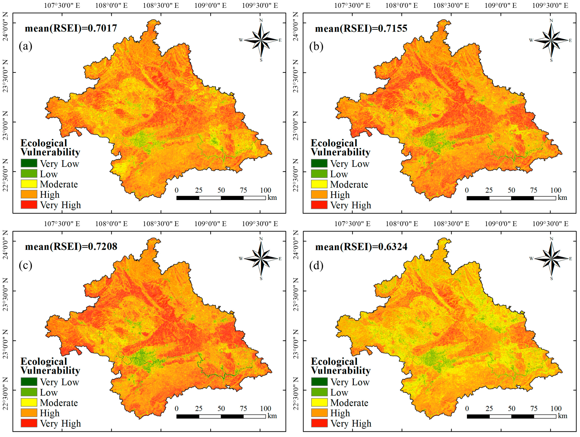
The statistical results are presented in

Table 8. The statistical results of the four ecological indicators and RSEI in different seasons.

Season	Indicator	NDVI	WET	NDBSI	LST	RSEI
Spring	Mean	0.756	0.823	0.396	0.726	0.704
	Standard deviation	0.113	0.024	0.090	0.043	0.127
	Correlation with RSEI	0.973	0.512	−0.786	−0.319	1.000
Summer	Mean	0.820	0.522	0.321	0.802	0.718
	Standard deviation	0.098	0.031	0.090	0.024	0.131
	Correlation with RSEI	0.957	0.627	−0.868	−0.407	1.000
Autumn	Mean	0.800	0.873	0.361	0.644	0.722
	Standard deviation	0.119	0.028	0.106	0.047	0.141
	Correlation with RSEI	0.951	0.656	−0.815	−0.607	1.000
Winter	Mean	0.717	0.566	0.403	0.612	0.634
	Standard deviation	0.117	0.033	0.121	0.056	0.140
	Correlation with RSEI	0.920	0.587	−0.791	−0.227	1.000

. Based on the average values of each indicator and their correlations with RSEI, it can be concluded that in different seasons, NDVI and WET had a positive impact on the ecological environment, while NDBSI and LST had a negative impact, which is consistent with ecological principles. The ranking of RSEI from highest to lowest across different seasons was as follows: autumn (0.722) > summer (0.718) > spring (0.704) > winter (0.634). In terms of ecological condition assessment, the RSEI values for different seasons in Nanning ranged from 0.6 to 0.8, indicating a good ecological environment in each season. Regarding vulnerability to disasters, autumn had the highest vulnerability, followed by summer and spring, while winter had the lowest vulnerability. Specifically, during autumn, Nanning had higher NDVI, the highest WET, and lower NDBSI and LST, indicating the best ecological conditions and the highest vulnerability of the ecological environment, which could lead to more severe damage and loss from wildfires. In winter, Nanning had the lowest NDVI, lower WET, the highest NDBSI, and lower LST, resulting in the poorest ecological conditions during this period. The potential damage and loss to the ecological environment from wildfire incidents may be relatively smaller.

4.2.2. Ecological Vulnerability Map

In order to quantitatively and visually analyze the vulnerability of the ecological environment in different seasons and its variations, this study classified the ecological vulnerability into five levels: very low [0, 0.2], low (0.2, 0.4], moderate (0.4, 0.6], high (0.6, 0.8], and very high (0.8, 1.0]. This classification allows us to better understand the state of the ecological environment and facilitates comparison and analysis of the vulnerability across different seasons.

From Figure 15, it can be seen that in each season, the central, eastern, and northwestern parts of Nanning had higher vegetation coverage compared to other areas and were less affected by human activities, indicating better ecological environmental quality in these regions. This also meant that when wildfire disasters occurred, these areas faced greater ecological vulnerability and potential threats. In contrast, the urban central areas of the southern, central-western, and northeastern parts of Nanning, which were more influenced by human activities, often had relatively lower vegetation coverage, resulting in poorer ecological quality. Therefore, these areas exhibited lower ecological vulnerability when wildfire disasters occurred. As shown in

Table 9. Statistics of wildfire risk zoning results for different seasons.

Season	Vulnerability Level	Percentage of Area (%)
Spring	Very low	0.008
	Low	3.289
	Moderate	15.186
	High	58.244
	Very high	23.273
Summer	Very low	0.224
	Low	3.687
	Moderate	11.762
	High	54.926
	Very high	29.401
Autumn	Very low	0.474
	Low	4.361
	Moderate	10.626
	High	51.615
	Very high	32.923
Winter	Very low	0.013
	Low	6.689
	Moderate	30.134
	High	53.812
	Very high	9.352

, among the four seasons, the areas with very high and high ecological vulnerability decreased in the following order: autumn (84.538%) > summer (84.327%) > spring (81.517%) > winter (63.164%). It could be observed that the areas with very high or high ecological vulnerability were larger in autumn and summer, indicating a more fragile ecological environment and a greater potential threat from wildfire disasters. The areas with high ecological vulnerability were the smallest in winter, indicating lower ecological vulnerability and less impact from wildfire disasters.

In conclusion, there are differences in ecological vulnerability across different seasons. Nanning exhibited better ecological conditions in autumn and summer, indicating that the ecological environment during these periods was more fragile and could potentially lead to more severe damage and losses when facing wildfire disasters. On the other hand, the ecological conditions were poorer in spring and winter, suggesting that the impact of wildfire disasters on the ecological environment during these seasons might be relatively smaller.

4.3. Wildfire Risk Assessment for the Ecological Environment

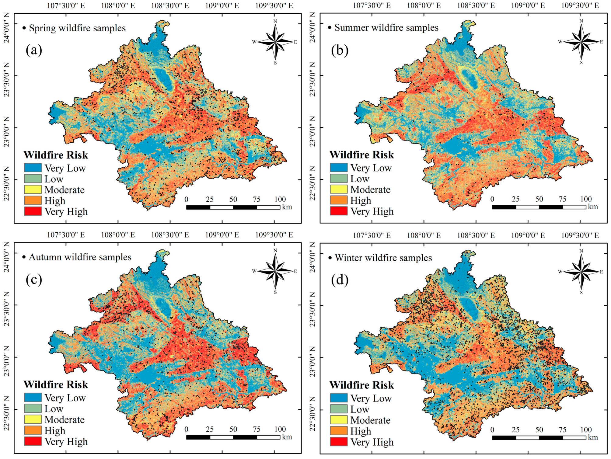
In this study, we utilized Equation (21) to integrate the assessment results of wildfire danger and ecological vulnerability in each season in Nanning in order to construct a wildfire risk assessment model for each season. Additionally, we adopted the equal interval approach to define risk classes to ensure that specific risk levels have the same range of wildfire risk values across all seasons, facilitating a consistent comparison of wildfire risk levels among different seasons. Based on the classification criteria of [0, 0.2], (0.2, 0.4], (0.4, 0.6], (0.6, 0.8], and (0.8, 1.0], the wildfire risk results for the entire region were divided into five risk levels: very low, low, moderate, high, and very high. The zoning results of wildfire risk are shown in Figure 16, and the percentages of different wildfire risk levels in each season are presented in

Table 10. Statistics of wildfire risk zoning results in different seasons.

Season	Risk Level	Percentage of Area (%)
Spring	Very low	21.897
	Low	14.272
	Moderate	16.259
	High	34.768
	Very high	12.804
Summer	Very low	22.420
	Low	16.842
	Moderate	16.897
	High	29.045
	Very high	14.796
Autumn	Very low	28.890
	Low	14.475
	Moderate	12.495
	High	24.097
	Very high	20.043
Winter	Very low	29.552
	Low	13.978
	Moderate	16.068
	High	33.497
	Very high	6.905

.

In the four seasons, the average wildfire risk in Nanning can be ranked from highest to lowest as follows: spring (0.4940) > summer (0.4827) > autumn (0.4662) > winter (0.4351). Furthermore, the areas with very high and high wildfire risk, from largest to smallest, were observed in spring (47.572%) > autumn (44.140%) > summer (43.841%) > winter (40.402%). The results indicate that in spring, Nanning faced a greater risk of wildfire-induced ecological damage, with a wider coverage of high risk areas posing a larger threat to the local ecological environment. Furthermore, although winter exhibited a higher danger to wildfires, it had the lowest ecological vulnerability, resulting in the lowest risk of ecological damage when wildfires occurred. Therefore, it is necessary to consider the varying levels of wildfire danger and ecological vulnerability across different seasons, summarize the patterns and spatial distribution characteristics of wildfire risk, and manage high-risk areas for wildfires separately for each season.

5. Discussion

5.1. SHAP Dependence Analysis of Nonseasonal Factors

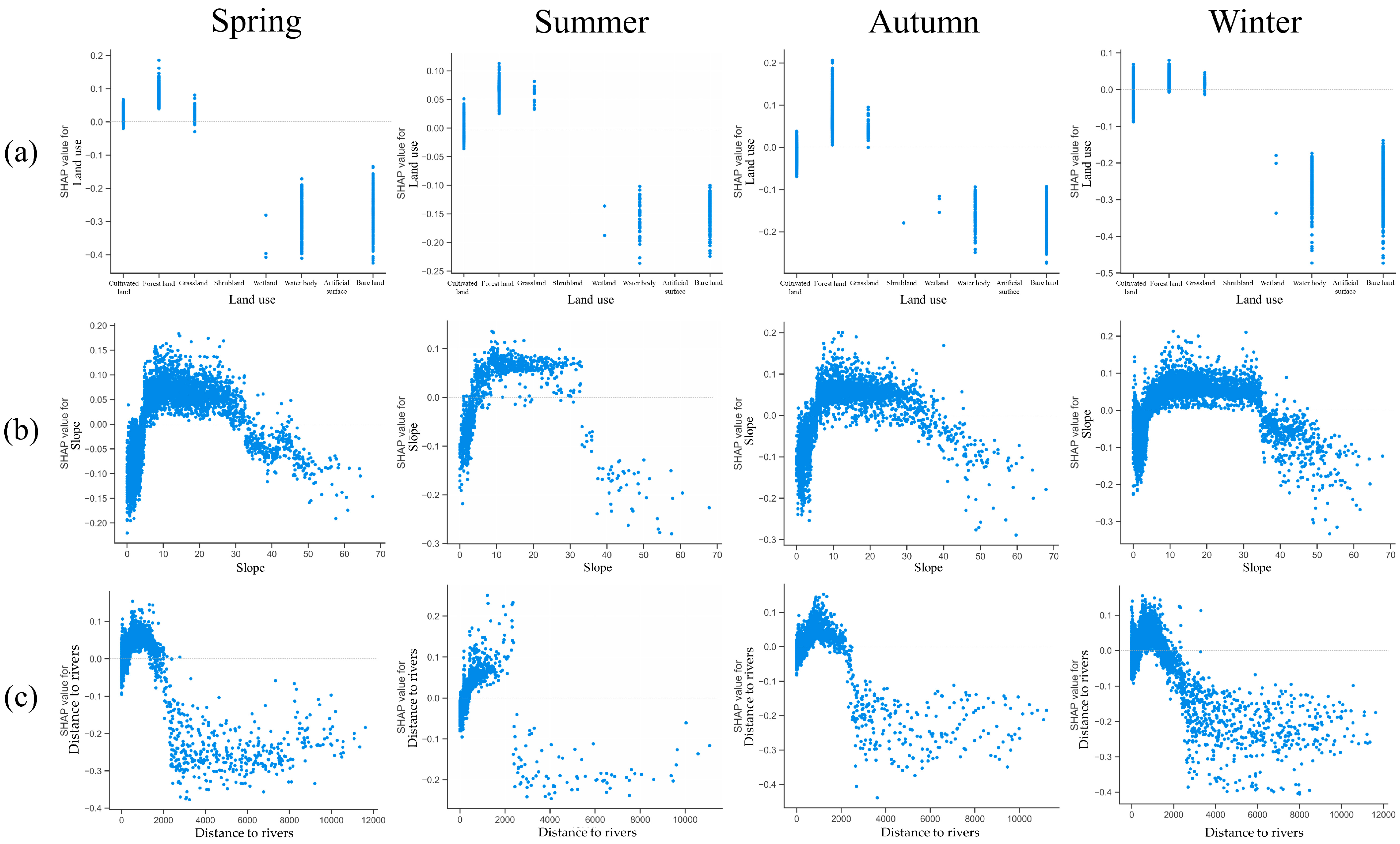
The research findings revealed that among all nonseasonal factors, land use, slope, and distance to rivers played a significant role in predicting wildfire danger across different seasons in Nanning. Utilizing the SHAP single dependency analysis method, we gained detailed insights into the impact of these factors on wildfire danger within various attribute intervals (Figure 17).

In terms of land use, we observed different trends in different seasons. In spring, the Shapley values for cultivated land, forest land, and grassland were generally greater than 0, indicating that these land use types are all susceptible to wildfire disaster. In contrast, the Shapley values of forest land and grassland remained high in summer, autumn, and winter, while cultivated land showed high Shapley values in only some samples. It is evident that forest land and grassland were more susceptible to wildfire impacts compared to cultivated land during these seasons.

In terms of slope, we discovered that in any season, the samples exhibited Shapley values greater than 0 when the slope exceeded 5° but remained below 30°. This suggests that steeper slopes contributed to rugged terrain, accelerating the spread of wildfires, and fuel accumulation. Consequently, areas with higher slopes were more prone to wildfire occurrences.

In terms of distance to rivers, we observed that when the distance was greater than 500 m but less than 2000 m, the samples exhibited positive Shapley values, indicating a higher danger of wildfires in these areas. It is evident that regions adjacent to rivers were less prone to fire incidents, while areas farther away from rivers but still maintaining a certain distance were more susceptible to wildfires. These areas likely harbored a greater abundance of flammable vegetation and combustible materials, thereby increasing the risk of wildfire spread and propagation.

On the whole, the Shapley value trends of slope and distance to rivers in different seasons are relatively consistent, indicating that their influence on wildfire danger remains relatively stable across seasons. However, for the same land use type, such as cultivated land, there are variations in the distribution of Shapley values among different seasons, suggesting that the impact of land use on wildfire danger varies across seasons. It is evident that seasonal factors play an important moderating role in explaining the influence of the other factors on wildfire danger in different seasons. This variability reminds us of the need to adopt appropriate prevention and management strategies in different seasons to address the potential risks of wildfires.

5.2. Comparison with Previous Studies

Wildfire danger assessment is a complex task involving multiple influencing factors and non-linear relationships, and traditional machine learning algorithms often struggle to provide explanations for model predictions [96]. The SHAP method, by calculating the Shapley values of features, quantifies the contribution of each feature to the prediction results, thus aiding in the interpretation of the model’s prediction process and outcomes [40]. In our study, we observed that slope, as an important terrain factor influencing wildfires, received extensive support in previous research [38,39,49]. Additionally, many studies emphasized the positive role of vegetation coverage in promoting wildfire occurrences, which aligns with our findings [38,49]. However, there are also studies suggesting a weaker impact of vegetation coverage, and even a negative relationship with wildfire occurrences [39]. Moreover, meteorological factors, such as temperature, have shown a significant positive impact on wildfire occurrences in some studies [37,49], while others have demonstrated an inverse result, with temperature having a minor negative effect on wildfires [39,97]. These discrepancies in wildfire danger assessment arise from differences in climate and vegetation coverage across regions, leading to variations in the assessment results. Furthermore, within the same region, the frequency of wildfire occurrences may change over time due to temporal variations in climate and vegetation coverage. Therefore, exploring the temporal and spatial patterns of wildfire danger based on seasons and understanding the complexity of influencing factors are of vital importance.

As of now, numerous scholars have conducted extensive research on wildfire danger within different seasons [12,20,50]. Their findings consistently show distinct spatial distributions of wildfire danger across different seasons in the same region, demonstrating that considering seasonal dimensions provides a more comprehensive identification of potentially high-danger areas. However, variations exist in the assessment results of seasonal wildfire danger among different regions. In our study, the distribution of high-danger wildfire areas was more widespread in spring and winter, with fewer areas in summer and autumn, which is in line with a previous study [12]. However, another study showed higher danger in spring and autumn [50]. Furthermore, some regions even exhibit a divide between winter wildfire states in the north and summer wildfire states in the south [20]. These observations indicate significant regional differences in wildfire danger influenced by seasonal changes. Different climate conditions, vegetation coverage, and terrain factors in distinct regions may result in varying patterns of wildfire danger across seasons. Therefore, to understand the wildfire occurrence patterns in different regions, it is essential to fully consider seasonal factors and to explore the reasons behind the seasonal differences, thereby enhancing the accuracy and effectiveness of wildfire prediction and response.

5.3. Significance of Different Dimensions of Wildfire Riskiness Assessment

Given the seasonal distribution patterns of wildfire incidents in Nanning and the influence of seasonal factors, conducting wildfire risk assessments for different seasons is of great significance. Assessing wildfire risks in different seasons can help us to gain a comprehensive understanding of fire risk conditions. Climate conditions and vegetation states vary across seasons, necessitating considerations of these factors’ fluctuations in wildfire risk assessments. In the study area, the frequency of wildfire incidents is higher in spring and winter, with a wider coverage of high-risk areas. Summer and autumn exhibit higher ecological conditions and vulnerability, making them more susceptible to wildfire impacts. Thus, notable differences exist in the danger and vulnerability assessments among different seasons.

In conclusion, due to the suddenness, destructiveness, and uncontrollability of wildfire incidents, as well as the influence of seasonal differences, conducting wildfire risk assessments for different seasons is necessary. By integrating assessments of wildfire danger and ecological vulnerability across different seasons, we can better understand the potential risks of wildfire-induced ecological losses in different seasons [20]. This understanding enables us to take the corresponding preventive measures, strengthen monitoring and emergency responses, reduce the impact of wildfire incidents on the ecological environment and society, and ensure the safety and quality of people’s lives.

5.4. Limitations and Future Works

This study has several limitations. Firstly, only four common seasonal factors, namely, NDVI, temperature, precipitation, and wind speed, were considered in this work. However, there are other factors that could be included in the wildfire danger assessment, such as solar radiation [98,99], soil moisture [12,100], and air humidity [44,101]. Secondly, the historical wildfire data provided by government agencies mainly focus on forest areas, and there is incomplete information about wildfire incidents in cultivated land and transitional vegetation areas. Therefore, this study advocates for the use of active fire data products [37]. Although the wildfire sample dataset has undergone rigorous quality control and screening, it may still need to be compared with imagery from sources such as Landsat 8, Sentinel, and other imagery data to further enhance the reliability of the wildfire samples.

Furthermore, it should be noted that the lightning activity factor was not included in our investigation of seasonal wildfire danger, which was a limitation of this study. Lightning activity plays a crucial role as a major natural ignition source in the formation and propagation of wildfires [102]. The process of lightning-induced fires is highly complex and closely related to factors such as vegetation type, fuel conditions, weather, and topography, with many aspects still remaining unknown [103]. Lightning-caused fires in specific regions often exhibit distinct spatiotemporal distribution patterns [104], and factors such as meteorology [105,106] (especially rainfall), combustible materials [107] (vegetation cover, vegetation type), and topography [108] significantly influence the frequency and intensity of wildfires caused by lightning activity [109]. In this study, based on consideration of seasonal factors such as topography, climate, and vegetation cover, we explored the spatiotemporal variation patterns of wildfire danger. Among the seasonal influencing factors, climate factors such as temperature, wind speed, and precipitation directly affect the probability of wildfire occurrence, while vegetation cover determines the fuel supply for wildfires [102]. The combined effects of these seasonal factors lead to considerable variations in wildfire danger across different seasons and regions. Therefore, considering the critical role of lightning activity in wildfire occurrence, future research could focus on studying the significant impact of lightning activity on wildfires and incorporate it into group of the factors for assessing wildfire danger. By collecting and compiling wildfire disaster data caused by lightning activity and integrating lightning activity factors with key factors such as topography, climate, and vegetation cover, we may enhance the predictive accuracy of models and gain a better understanding of the spatial distribution and seasonal variation of wildfires. Moreover, exploring the interaction between lightning activity and climate factors can further elucidate the relationship between wildfire danger and climate change. Through in-depth research on the impact of climate factors and lightning activity on wildfire danger, we will come to better understand the potential influence of climate change on wildfire risk, providing scientific evidence for wildfire disaster management and mitigation.

6. Conclusions

This study focused on Nanning as the research area. Firstly, both nonseasonal and seasonal factors related to wildfires were collected. The historical wildfire samples and seasonal factors were divided into five different periods: all seasons, spring, summer, autumn, and winter, forming separate datasets. Based on an ML algorithm, we constructed wildfire danger models within different periods, explored the advantages of wildfire danger analysis and evaluation based on seasonal dimensions, and systematically understood the seasonal change patterns of spatial distribution of wildfire danger and the differences in the roles of various factors. In addition, we constructed ecological vulnerability models for different seasons based on greenness, heat, dryness, and wetness indicators, and analyzed the ecological vulnerability situation and spatial distribution characteristics in different seasons. Finally, the results of vulnerability and danger evaluation were integrated to construct the wildfire disaster risk model, and the potential threat of wildfire to the local ecological environment in different seasons was systematically evaluated. The conclusions of the study are as follows:

(1)

The occurrence of wildfire disaster in Nanning is mainly influenced by seasonal factors. The evaluation and analysis of wildfire danger in Nanning based on each season can obtain wildfire danger evaluation results with a better prediction performance. This makes up for the shortcomings of traditional evaluation methods and can grasp the spatial and temporal distribution patterns of wildfires in the area in a more refined way.

(2)

The wildfires in Nanning mainly occurred in spring and winter, reflecting most of the high-wildfire-danger areas in the region, while the high-wildfire-danger areas in summer and autumn accounted for a relatively small proportion. In each season, NDVI was the most critical factor affecting wildfire danger, while slope was the most important nonseasonal factor. Evaluating wildfire danger based on each season can capture the differences in the roles of factors that have a major impact on wildfire occurrence in different seasons in a more refined way.

(3)

The ecological vulnerability of Nanning is higher in autumn and summer, with a larger area occupied by high vulnerability zones. This indicates a greater potential threat of wildfire disasters to the ecological environment in Nanning. The ecological vulnerability is lower in spring and winter, resulting in a relatively smaller impact of wildfire disasters on the ecological environment during these periods.

(4)

The ecological environment of Nanning faces the most severe wildfire risk during the spring period and the lowest wildfire risk during the winter period. A comprehensive consideration of wildfire danger and ecological vulnerability in different seasons enables a more comprehensive assessment of the degree of risk of damage to the ecological environment caused by wildfire disasters. This enables swift responses to be made and effective measures to be taken during wildfire incidents, minimizing the damage to the ecological environment to the greatest extent possible.

References

1. Hong, H.; Jaafari, A.; Zenner, E.K. Predicting spatial patterns of wildfire susceptibility in the Huichang County, China: An integrated model to analysis of landscape indicators. Ecol. Indic. 2019, 101, 878–891. [Google Scholar]
2. Stephens, S.L.; Agee, J.K.; Fule, P.Z.; North, M.; Romme, W.; Swetnam, T.; Turner, M.G. Managing forests and fire in changing climates. Science 2013, 342, 41–42. [Google Scholar] [CrossRef]
3. Nami, M.; Jaafari, A.; Fallah, M.; Nabiuni, S. Spatial prediction of wildfire probability in the Hyrcanian ecoregion using evidential belief function model and GIS. Int. J. Environ. Sci. Technol. 2018, 15, 373–384. [Google Scholar]
4. Bardsley, D.; Weber, D.; Robinson, G.; Moskwa, E.; Bardsley, A. Wildfire risk, biodiversity and peri-urban planning in the Mt Lofty Ranges, South Australia. Appl. Geogr. 2015, 63, 155–165. [Google Scholar]
5. García-Llamas, P.; Suárez-Seoane, S.; Taboada, A.; Fernández-Manso, A.; Quintano, C.; Fernández-García, V.; Fernández-Guisuraga, J.M.; Marcos, E.; Calvo, L. Environmental drivers of fire severity in extreme fire events that affect Mediterranean pine forest ecosystems. For. Ecol. Manag. 2019, 433, 24–32. [Google Scholar]
6. Venkatesh, K.; Preethi, K.; Ramesh, H. Evaluating the effects of forest fire on water balance using fire susceptibility maps. Ecol. Indic. 2020, 110, 105856. [Google Scholar] [CrossRef]
7. Dove, N.C.; Safford, H.D.; Bohlman, G.N.; Estes, B.L.; Hart, S.C. High-severity wildfire leads to multi-decadal impacts on soil biogeochemistry in mixed-conifer forests. Ecol. Appl. 2020, 30, e02072. [Google Scholar] [CrossRef]
8. Di Napoli, M.; Marsiglia, P.; Di Martire, D.; Ramondini, M.; Ullo, S.L.; Calcaterra, D. Landslide susceptibility assessment of wildfire burnt areas through earth-observation techniques and a machine learning-based approach. Remote Sens. 2020, 12, 2505. [Google Scholar]
9. He, Q.; Jiang, Z.; Wang, M.; Liu, K. Landslide and wildfire susceptibility assessment in southeast asia using ensemble machine learning methods. Remote Sens. 2021, 13, 1572. [Google Scholar] [CrossRef]
10. Zema, D.A.; Nunes, J.P.; Lucas-Borja, M.E. Improvement of seasonal runoff and soil loss predictions by the MMF (Morgan-Morgan-Finney) model after wildfire and soil treatment in Mediterranean forest ecosystems. Catena 2020, 188, 104415. [Google Scholar]
11. Xie, L.; Zhang, R.; Zhan, J.; Li, S.; Shama, A.; Zhan, R.; Wang, T.; Lv, J.; Bao, X.; Wu, R. Wildfire risk assessment in Liangshan Prefecture, China based on an integration machine learning algorithm. Remote Sens. 2022, 14, 4592. [Google Scholar] [CrossRef]
12. Wang, W.; Zhao, F.; Wang, Y.; Huang, X.; Ye, J. Seasonal differences in the spatial patterns of wildfire drivers and susceptibility in the southwest mountains of China. Sci. Total Environ. 2023, 869, 161782. [Google Scholar] [CrossRef]
13. Shafapourtehrany, M. Geospatial Wildfire Risk Assessment from Social, Infrastructural and Environmental Perspectives: A Case Study in Queensland Australia. Fire 2023, 6, 22. [Google Scholar] [CrossRef]
14. Nikolić, G.; Vujović, F.; Golijanin, J.; Šiljeg, A.; Valjarević, A. Modelling of Wildfire Susceptibility in Different Climate Zones in Montenegro Using GIS-MCDA. Atmosphere 2023, 14, 929. [Google Scholar] [CrossRef]
15. Hardy, C.C. Wildland fire hazard and risk: Problems, definitions, and context. For. Ecol. Manag. 2005, 211, 73–82. [Google Scholar] [CrossRef]
16. Shah, M.A.R.; Renaud, F.G.; Anderson, C.C.; Wild, A.; Domeneghetti, A.; Polderman, A.; Votsis, A.; Pulvirenti, B.; Basu, B.; Thomson, C. A review of hydro-meteorological hazard, vulnerability, and risk assessment frameworks and indicators in the context of nature-based solutions. Int. J. Disaster Risk Reduct. 2020, 50, 101728. [Google Scholar] [CrossRef]
17. Van Westen, C.J. Remote sensing and GIS for natural hazards assessment and disaster risk management. Treatise Geomorphol. 2013, 3, 259–298. [Google Scholar]
18. Ghorbanzadeh, O.; Blaschke, T.; Gholamnia, K.; Aryal, J. Forest fire susceptibility and risk mapping using social/infrastructural vulnerability and environmental variables. Fire 2019, 2, 50. [Google Scholar] [CrossRef] [Green Version]
19. Zacharakis, I.; Tsihrintzis, V.A. Integrated wildfire danger models and factors: A review. Sci. Total Environ. 2023, 899, 165704. [Google Scholar]
20. Tang, X.; Machimura, T.; Li, J.; Yu, H.; Liu, W. Evaluating seasonal wildfire susceptibility and wildfire threats to local ecosystems in the largest forested area of China. Earth’s Future 2022, 10, e2021EF002199. [Google Scholar] [CrossRef]
21. Molina, J.R.; Rodríguez y Silva, F.; Herrera, M.Á. Economic vulnerability of fire-prone landscapes in protected natural areas: Application in a Mediterranean Natural Park. Eur. J. For. Res. 2017, 136, 609–624. [Google Scholar]
22. Jaafari, A.; Gholami, D.M.; Zenner, E.K. A Bayesian modeling of wildfire probability in the Zagros Mountains, Iran. Ecol. Inform. 2017, 39, 32–44. [Google Scholar] [CrossRef]
23. Kondylatos, S.; Prapas, I.; Ronco, M.; Papoutsis, I.; Camps-Valls, G.; Piles, M.; Fernández-Torres, M.Á.; Carvalhais, N. Wildfire danger prediction and understanding with Deep Learning. Geophys. Res. Lett. 2022, 49, e2022GL099368. [Google Scholar] [CrossRef]
24. Singh, M.; Huang, Z. Analysis of forest fire dynamics, distribution and main drivers in the Atlantic Forest. Sustainability 2022, 14, 992. [Google Scholar] [CrossRef]
25. Dhar, T.; Bhatta, B.; Aravindan, S. Forest fire occurrence, distribution and risk mapping using geoinformation technology: A case study in the sub-tropical forest of the Meghalaya, India. Remote Sens. Appl. Soc. Environ. 2023, 29, 100883. [Google Scholar]
26. Rezaie-Balf, M.; Ghaemi, A.; Jun, C.; Band, S.; Bateni, S.M. Towards an integrative, spatially-explicit modeling for flash floods susceptibility mapping based on remote sensing and flood inventory data in Southern Caspian Sea Littoral, Iran. Geocarto Int. 2022, 37, 12638–12668. [Google Scholar] [CrossRef]
27. Hai, T.; Theruvil Sayed, B.; Majdi, A.; Zhou, J.; Sagban, R.; Band, S.S.; Mosavi, A. An integrated GIS-based multivariate adaptive regression splines-cat swarm optimization for improving the accuracy of wildfire susceptibility mapping. Geocarto Int. 2023, 2, 2167005. [Google Scholar] [CrossRef]
28. Ljubomir, G.; Pamučar, D.; Drobnjak, S.; Pourghasemi, H.R. Modeling the spatial variability of forest fire susceptibility using geographical information systems and the analytical hierarchy process. In Spatial Modeling in GIS and R for Earth and Environmental Sciences; Elsevier: Amsterdam, The Netherlands, 2019; pp. 337–369. [Google Scholar]
29. Jain, P.; Coogan, S.C.; Subramanian, S.G.; Crowley, M.; Taylor, S.; Flannigan, M.D. A review of machine learning applications in wildfire science and management. Environ. Rev. 2020, 28, 478–505. [Google Scholar] [CrossRef]
30. Mohammadi, F.; Bavaghar, M.P.; Shabanian, N. Forest fire risk zone modeling using logistic regression and GIS: An Iranian case study. Small-Scale For. 2014, 13, 117–125. [Google Scholar]
31. Cao, Y.; Wang, M.; Liu, K. Wildfire susceptibility assessment in Southern China: A comparison of multiple methods. Int. J. Disaster Risk Sci. 2017, 8, 164–181. [Google Scholar]
32. Tang, X.; Machimura, T.; Li, J.; Liu, W.; Hong, H. A novel optimized repeatedly random undersampling for selecting negative samples: A case study in an SVM-based forest fire susceptibility assessment. J. Environ. Manag. 2020, 271, 111014. [Google Scholar]
33. Bustillo Sánchez, M.; Tonini, M.; Mapelli, A.; Fiorucci, P. Spatial assessment of wildfires susceptibility in Santa Cruz (Bolivia) using random forest. Geosciences 2021, 11, 224. [Google Scholar] [CrossRef]
34. Zhang, G.; Wang, M.; Liu, K. Deep neural networks for global wildfire susceptibility modelling. Ecol. Indic. 2021, 127, 107735. [Google Scholar] [CrossRef]
35. Lan, Y.; Wang, J.; Hu, W.; Kurbanov, E.; Cole, J.; Sha, J.; Jiao, Y.; Zhou, J. Spatial pattern prediction of forest wildfire susceptibility in Central Yunnan Province, China based on multivariate data. Nat. Hazards 2023, 116, 565–586. [Google Scholar] [CrossRef]
36. Jaafari, A.; Zenner, E.K.; Panahi, M.; Shahabi, H. Hybrid artificial intelligence models based on a neuro-fuzzy system and metaheuristic optimization algorithms for spatial prediction of wildfire probability. Agric. For. Meteorol. 2019, 266, 198–207. [Google Scholar] [CrossRef]
37. Iban, M.C.; Sekertekin, A. Machine learning based wildfire susceptibility mapping using remotely sensed fire data and GIS: A case study of Adana and Mersin provinces, Turkey. Ecol. Inform. 2022, 69, 101647. [Google Scholar]
38. Cilli, R.; Elia, M.; D’Este, M.; Giannico, V.; Amoroso, N.; Lombardi, A.; Pantaleo, E.; Monaco, A.; Sanesi, G.; Tangaro, S. Explainable artificial intelligence (XAI) detects wildfire occurrence in the Mediterranean countries of Southern Europe. Sci. Rep. 2022, 12, 16349. [Google Scholar] [CrossRef]
39. Abdollahi, A.; Pradhan, B. Explainable artificial intelligence (XAI) for interpreting the contributing factors feed into the wildfire susceptibility prediction model. Sci. Total Environ. 2023, 879, 163004. [Google Scholar] [CrossRef]
40. Cheng, X.; Wang, J.; Li, H.; Zhang, Y.; Wu, L.; Liu, Y. A method to evaluate task-specific importance of spatio-temporal units based on explainable artificial intelligence. Int. J. Geogr. Inf. Sci. 2021, 35, 2002–2025. [Google Scholar] [CrossRef]
41. Lundberg, S.M.; Erion, G.G.; Lee, S.-I. Consistent individualized feature attribution for tree ensembles. arXiv 2018, arXiv:1802.03888. [Google Scholar]
42. Zhou, X.; Wen, H.; Li, Z.; Zhang, H.; Zhang, W. An interpretable model for the susceptibility of rainfall-induced shallow landslides based on SHAP and XGBoost. Geocarto Int. 2022, 37, 13419–13450. [Google Scholar] [CrossRef]
43. Bergonse, R.; Oliveira, S.; Gonçalves, A.; Nunes, S.; da Câmara, C.; Zêzere, J.L. A combined structural and seasonal approach to assess wildfire susceptibility and hazard in summertime. Nat. Hazards 2021, 106, 2545–2573. [Google Scholar] [CrossRef]
44. Bergonse, R.; Oliveira, S.; Gonçalves, A.; Nunes, S.; DaCamara, C.; Zêzere, J.L. Predicting burnt areas during the summer season in Portugal by combining wildfire susceptibility and spring meteorological conditions. Geomat. Nat. Hazards Risk 2021, 12, 1039–1057. [Google Scholar] [CrossRef]
45. Flannigan, M.D.; Krawchuk, M.A.; de Groot, W.J.; Wotton, B.M.; Gowman, L.M. Implications of changing climate for global wildland fire. Int. J. Wildland Fire 2009, 18, 483–507. [Google Scholar] [CrossRef]
46. Vacchiano, G.; Foderi, C.; Berretti, R.; Marchi, E.; Motta, R. Modeling anthropogenic and natural fire ignitions in an inner-alpine valley. Nat. Hazards Earth Syst. Sci. 2018, 18, 935–948. [Google Scholar] [CrossRef] [Green Version]
47. Jhariya, M.K.; Raj, A. Effects of wildfires on flora, fauna and physico-chemical properties of soil—An overview. J. Appl. Nat. Sci. 2014, 6, 887–897. [Google Scholar] [CrossRef] [Green Version]
48. Dunn, C.J.; D O’Connor, C.; Abrams, J.; Thompson, M.P.; Calkin, D.E.; Johnston, J.D.; Stratton, R.; Gilbertson-Day, J. Wildfire risk science facilitates adaptation of fire-prone social-ecological systems to the new fire reality. Environ. Res. Lett. 2020, 15, 025001. [Google Scholar] [CrossRef]
49. Yue, W.; Ren, C.; Liang, Y.; Liang, J.; Lin, X.; Yin, A.; Wei, Z. Assessment of Wildfire Susceptibility and Wildfire Threats to Ecological Environment and Urban Development Based on GIS and Multi-Source Data: A Case Study of Guilin, China. Remote Sens. 2023, 15, 2659. [Google Scholar]
50. Trucchia, A.; Meschi, G.; Fiorucci, P.; Gollini, A.; Negro, D. Defining wildfire susceptibility maps in Italy for understanding seasonal wildfire regimes at the national level. Fire 2022, 5, 30. [Google Scholar] [CrossRef]
51. Schroeder, W.; Oliva, P.; Giglio, L.; Csiszar, I.A. The New VIIRS 375 m active fire detection data product: Algorithm description and initial assessment. Remote Sens. Environ. 2014, 143, 85–96. [Google Scholar]
52. Gürsoy, M.İ.; Orhan, O.; Tekin, S. Creation of wildfire susceptibility maps in the Mediterranean Region (Turkey) using convolutional neural networks and multilayer perceptron techniques. For. Ecol. Manag. 2023, 538, 121006. [Google Scholar] [CrossRef]
53. Li, F.; Zhang, X.; Kondragunta, S.; Csiszar, I. Comparison of fire radiative power estimates from VIIRS and MODIS observations. J. Geophys. Res. Atmos. 2018, 123, 4545–4563. [Google Scholar] [CrossRef]
54. Nur, A.S.; Kim, Y.J.; Lee, J.H.; Lee, C.-W. Spatial Prediction of Wildfire Susceptibility Using Hybrid Machine Learning Models Based on Support Vector Regression in Sydney, Australia. Remote Sens. 2023, 15, 760. [Google Scholar] [CrossRef]
55. Fernández-Manso, A.; Quintano, C. A synergetic approach to burned area mapping using maximum entropy modeling trained with hyperspectral data and VIIRS hotspots. Remote Sens. 2020, 12, 858. [Google Scholar] [CrossRef] [Green Version]
56. Guo, F.; Selvalakshmi, S.; Lin, F.; Wang, G.; Wang, W.; Su, Z.; Liu, A. Geospatial information on geographical and human factors improved anthropogenic fire occurrence modeling in the Chinese boreal forest. Can. J. For. Res. 2016, 46, 582–594. [Google Scholar] [CrossRef] [Green Version]
57. Vadrevu, K.P.; Eaturu, A.; Badarinath, K. Fire risk evaluation using multicriteria analysis—A case study. Environ. Monit. Assess. 2010, 166, 223–239. [Google Scholar] [CrossRef] [PubMed]
58. Razavi-Termeh, S.V.; Sadeghi-Niaraki, A.; Choi, S.-M. Gully erosion susceptibility mapping using artificial intelligence and statistical models. Geomat. Nat. Hazards Risk 2020, 11, 821–844. [Google Scholar] [CrossRef]
59. Kalantar, B.; Ueda, N.; Idrees, M.O.; Janizadeh, S.; Ahmadi, K.; Shabani, F. Forest fire susceptibility prediction based on machine learning models with resampling algorithms on remote sensing data. Remote Sens. 2020, 12, 3682. [Google Scholar] [CrossRef]
60. Ghorbanzadeh, O.; Valizadeh Kamran, K.; Blaschke, T.; Aryal, J.; Naboureh, A.; Einali, J.; Bian, J. Spatial prediction of wildfire susceptibility using field survey gps data and machine learning approaches. Fire 2019, 2, 43. [Google Scholar] [CrossRef] [Green Version]
61. Sachdeva, S.; Bhatia, T.; Verma, A. GIS-based evolutionary optimized Gradient Boosted Decision Trees for forest fire susceptibility mapping. Nat. Hazards 2018, 92, 1399–1418. [Google Scholar] [CrossRef]
62. De Santana, R.O.; Delgado, R.C.; Schiavetti, A. Modeling susceptibility to forest fires in the Central Corridor of the Atlantic Forest using the frequency ratio method. J. Environ. Manag. 2021, 296, 113343. [Google Scholar] [CrossRef] [PubMed]
63. Verde, J.; Zêzere, J. Assessment and validation of wildfire susceptibility and hazard in Portugal. Nat. Hazards Earth Syst. Sci. 2010, 10, 485–497. [Google Scholar] [CrossRef]
64. Naderpour, M.; Rizeei, H.M.; Ramezani, F. Forest fire risk prediction: A spatial deep neural network-based framework. Remote Sens. 2021, 13, 2513. [Google Scholar] [CrossRef]
65. Eskandari, S.; Pourghasemi, H.R.; Tiefenbacher, J.P. Fire-susceptibility mapping in the natural areas of Iran using new and ensemble data-mining models. Environ. Sci. Pollut. Res. 2021, 28, 47395–47406. [Google Scholar] [CrossRef]
66. Xu, H.; Wang, M.; Shi, T.; Guan, H.; Fang, C.; Lin, Z. Prediction of ecological effects of potential population and impervious surface increases using a remote sensing based ecological index (RSEI). Ecol. Indic. 2018, 93, 730–740. [Google Scholar] [CrossRef]
67. Xu, H.; Wang, Y.; Guan, H.; Shi, T.; Hu, X. Detecting ecological changes with a remote sensing based ecological index (RSEI) produced time series and change vector analysis. Remote Sens. 2019, 11, 2345. [Google Scholar] [CrossRef] [Green Version]
68. Yang, Y.; Li, H.; Qian, C. Analysis of the implementation effects of ecological restoration projects based on carbon storage and eco-environmental quality: A case study of the Yellow River Delta, China. J. Environ. Manag. 2023, 340, 117929. [Google Scholar]
69. Han, N.; Hu, K.; Yu, M.; Jia, P.; Zhang, Y. Incorporating Ecological Constraints into the Simulations of Tropical Urban Growth Boundaries: A Case Study of Sanya City on Hainan Island, China. Appl. Sci. 2022, 12, 6409. [Google Scholar]
70. Xu, H. A remote sensing index for assessment of regional ecological changes. China Environ. Sci. 2013, 33, 889–897. [Google Scholar]
71. Zheng, Z.; Wu, Z.; Chen, Y.; Yang, Z.; Marinello, F. Exploration of eco-environment and urbanization changes in coastal zones: A case study in China over the past 20 years. Ecol. Indic. 2020, 119, 106847. [Google Scholar]
72. Goward, S.N.; Xue, Y.; Czajkowski, K.P. Evaluating land surface moisture conditions from the remotely sensed temperature/vegetation index measurements: An exploration with the simplified simple biosphere model. Remote Sens. Environ. 2002, 79, 225–242. [Google Scholar]
73. Liu, T.; Ren, C.; Zhang, S.; Yin, A.; Yue, W. Coupling Coordination Analysis of Urban Development and Ecological Environment in Urban Area of Guilin Based on Multi-Source Data. Int. J. Environ. Res. Public Health 2022, 19, 12583. [Google Scholar] [CrossRef] [PubMed]
74. Xu, H. A new index for delineating built-up land features in satellite imagery. Int. J. Remote Sens. 2008, 29, 4269–4276. [Google Scholar] [CrossRef]
75. Rikimaru, A.; Roy, P.; Miyatake, S. Tropical forest cover density mapping. Trop. Ecol. 2002, 43, 39–47. [Google Scholar]
76. Crist, E.P.; Cicone, R.C. A physically-based transformation of Thematic Mapper data—The TM Tasseled Cap. IEEE Trans. Geosci. Remote Sens. 1984, GE-22, 256–263. [Google Scholar] [CrossRef]
77. Ke, G.; Meng, Q.; Finley, T.; Wang, T.; Chen, W.; Ma, W.; Ye, Q.; Liu, T.-Y. Lightgbm: A highly efficient gradient boosting decision tree. Adv. Neural Inf. Process. Syst. 2017, 30, 3149–3157. [Google Scholar]
78. Sun, Y.; Zhang, F.; Lin, H.; Xu, S. A Forest Fire Susceptibility Modeling Approach Based on Light Gradient Boosting Machine Algorithm. Remote Sens. 2022, 14, 4362. [Google Scholar] [CrossRef]
79. Abujayyab, S.K.; Kassem, M.M.; Khan, A.A.; Wazirali, R.; Coşkun, M.; Taşoğlu, E.; Öztürk, A.; Toprak, F. Wildfire Susceptibility Mapping Using Five Boosting Machine Learning Algorithms: The Case Study of the Mediterranean Region of Turkey. Adv. Civ. Eng. 2022, 2022, 3959150. [Google Scholar]
80. Ling, C.X.; Huang, J.; Zhang, H. AUC: A better measure than accuracy in comparing learning algorithms. In Proceedings of the Advances in Artificial Intelligence: 16th Conference of the Canadian Society for Computational Studies of Intelligence, AI 2003, Halifax, NS, Canada, 11–13 June 2003; pp. 329–341. [Google Scholar]
81. Zhang, G.; Wang, M.; Liu, K. Forest fire susceptibility modeling using a convolutional neural network for Yunnan province of China. Int. J. Disaster Risk Sci. 2019, 10, 386–403. [Google Scholar] [CrossRef] [Green Version]
82. Akıncı, H.A.; Akıncı, H. Machine learning based forest fire susceptibility assessment of Manavgat district (Antalya), Turkey. Earth Sci. Inform. 2023, 16, 397–414. [Google Scholar] [CrossRef]
83. Bui, D.T.; Bui, Q.-T.; Nguyen, Q.-P.; Pradhan, B.; Nampak, H.; Trinh, P.T. A hybrid artificial intelligence approach using GIS-based neural-fuzzy inference system and particle swarm optimization for forest fire susceptibility modeling at a tropical area. Agric. For. Meteorol. 2017, 233, 32–44. [Google Scholar]
84. Kantarcioglu, O.; Kocaman, S.; Schindler, K. Artificial neural networks for assessing forest fire susceptibility in Türkiye. Ecol. Inform. 2023, 75, 102034. [Google Scholar] [CrossRef]
85. Mangalathu, S.; Hwang, S.-H.; Jeon, J.-S. Failure mode and effects analysis of RC members based on machine-learning-based SHapley Additive exPlanations (SHAP) approach. Eng. Struct. 2020, 219, 110927. [Google Scholar] [CrossRef]
86. Kannangara, K.P.M.; Zhou, W.; Ding, Z.; Hong, Z. Investigation of feature contribution to shield tunneling-induced settlement using Shapley additive explanations method. J. Rock Mech. Geotech. Eng. 2022, 14, 1052–1063. [Google Scholar]
87. UN DHA. Internationally Agreed Glossary of Basic Terms Related to Disaster Management; UN DHA (United Nations Department of Humanitarian Affairs): Geneva, Switzerland, 1992. [Google Scholar]
88. Xu, H.; Li, C.; Shi, T. Is the z-score standardized RSEI suitable for time-series ecological change detection? Comment on Zheng et al. (2022). Sci. Total Environ. 2022, 853, 158582. [Google Scholar] [CrossRef]
89. He, B.; Han, F.; Han, J.; Ren, Q.; Li, Y. The Ecological Evolution Analysis of Heritage Sites Based on The Remote Sensing Ecological Index—A Case Study of Kalajun–Kuerdening World Natural Heritage Site. Remote Sens. 2023, 15, 1179. [Google Scholar] [CrossRef]
90. Lu, C.; Shi, L.; Fu, L.; Liu, S.; Li, J.; Mo, Z. Urban Ecological Environment Quality Evaluation and Territorial Spatial Planning Response: Application to Changsha, Central China. Int. J. Environ. Res. Public Health 2023, 20, 3753. [Google Scholar] [PubMed]
91. Knight, F.H. Risk, Uncertainty and Profit; Houghton Mifflin: Boston, MA, USA, 1921; Volume 31. [Google Scholar]
92. Merz, B.; Aerts, J.; Arnbjerg-Nielsen, K.; Baldi, M.; Becker, A.; Bichet, A.; Blöschl, G.; Bouwer, L.M.; Brauer, A.; Cioffi, F. Floods and climate: Emerging perspectives for flood risk assessment and management. Nat. Hazards Earth Syst. Sci. 2014, 14, 1921–1942. [Google Scholar]
93. Jiménez-Perálvarez, J. Landslide-risk mapping in a developing hilly area with limited information on landslide occurrence. Landslides 2018, 15, 741–752. [Google Scholar] [CrossRef]
94. Azzimonti, O.L.; Colleoni, M.; De Amicis, M.; Frigerio, I. Combining hazard, social vulnerability and resilience to provide a proposal for seismic risk assessment. J. Risk Res. 2020, 23, 1225–1241. [Google Scholar] [CrossRef]
95. Zêzere, J.; Garcia, R.; Oliveira, S.; Reis, E. Probabilistic landslide risk analysis considering direct costs in the area north of Lisbon (Portugal). Geomorphology 2008, 94, 467–495. [Google Scholar] [CrossRef]
96. Arrieta, A.B.; Díaz-Rodríguez, N.; Del Ser, J.; Bennetot, A.; Tabik, S.; Barbado, A.; García, S.; Gil-López, S.; Molina, D.; Benjamins, R. Explainable Artificial Intelligence (XAI): Concepts, taxonomies, opportunities and challenges toward responsible AI. Inf. Fusion 2020, 58, 82–115. [Google Scholar]
97. Kang, Y.; Jang, E.; Im, J.; Kwon, C.; Kim, S. Developing a new hourly forest fire risk index based on catboost in South Korea. Appl. Sci. 2020, 10, 8213. [Google Scholar] [CrossRef]
98. Gholamnia, K.; Gudiyangada Nachappa, T.; Ghorbanzadeh, O.; Blaschke, T. Comparisons of diverse machine learning approaches for wildfire susceptibility mapping. Symmetry 2020, 12, 604. [Google Scholar] [CrossRef] [Green Version]
99. Al-Fugara, A.k.; Mabdeh, A.N.; Ahmadlou, M.; Pourghasemi, H.R.; Al-Adamat, R.; Pradhan, B.; Al-Shabeeb, A.R. Wildland fire susceptibility mapping using support vector regression and adaptive neuro-fuzzy inference system-based whale optimization algorithm and simulated annealing. ISPRS Int. J. Geo-Inf. 2021, 10, 382. [Google Scholar]
100. Sadatrazavi, A.; Motlagh, M.S.; Noorpoor, A.; Ehsani, A.H. Predicting Wildfires Occurrences Using Meteorological Parameters. Int. J. Environ. Res. 2022, 16, 106. [Google Scholar] [CrossRef]
101. Nhongo, E.J.S.; Fontana, D.C.; Guasselli, L.A.; Bremm, C. Probabilistic modelling of wildfire occurrence based on logistic regression, Niassa Reserve, Mozambique. Geomat. Nat. Hazards Risk 2019, 10, 1772–1792. [Google Scholar] [CrossRef] [Green Version]
102. Pausas, J.G.; Keeley, J.E. Wildfires and global change. Front. Ecol. Environ. 2021, 19, 387–395. [Google Scholar] [CrossRef]
103. Fernandes, P.M.; Santos, J.A.; Castedo-Dorado, F.; Almeida, R. Fire from the Sky in the Anthropocene. Fire 2021, 4, 13. [Google Scholar] [CrossRef]
104. Aldersley, A.; Murray, S.J.; Cornell, S.E. Global and regional analysis of climate and human drivers of wildfire. Sci. Total Environ. 2011, 409, 3472–3481. [Google Scholar] [CrossRef]
105. Price, C. Will a drier climate result in more lightning? Atmos. Res. 2009, 91, 479–484. [Google Scholar] [CrossRef]
106. Nampak, H.; Love, P.; Fox-Hughes, P.; Watson, C.; Aryal, J.; Harris, R.M. Characterizing spatial and temporal variability of lightning activity associated with wildfire over Tasmania, Australia. Fire 2021, 4, 10. [Google Scholar] [CrossRef]
107. Archibald, S.; Roy, D.P.; van Wilgen, B.W.; Scholes, R.J. What limits fire? An examination of drivers of burnt area in Southern Africa. Glob. Change Biol. 2009, 15, 613–630. [Google Scholar] [CrossRef] [Green Version]
108. Conedera, M.; Cesti, G.; Pezzatti, G.; Zumbrunnen, T.; Spinedi, F. Lightning-induced fires in the Alpine region: An increasing problem. For. Ecol. Manag. 2006, 234, S68. [Google Scholar] [CrossRef]
109. Jiao, Q.; Fan, M.; Tao, J.; Wang, W.; Liu, D.; Wang, P. Forest fire patterns and lightning-caused forest fire detection in Heilongjiang Province of China using satellite data. Fire 2023, 6, 166. [Google Scholar] [CrossRef]
Figure 1. Study area and spatial and temporal distribution of historical wildfires: (a) study area and the spatial distribution of historical wildfire samples; (b) total number of wildfire samples in each month from 2013 to 2022.
Forests 14 01616 g001
Figure 2. Nonseasonal driving factors: (a) elevation, (b) slope, (c) aspect, (d) curvature, (e) TWI, and (f) SPI.
Forests 14 01616 g002
Figure 3. Nonseasonal driving factors: (a) distance to roads, (b) distance to rivers, (c) population density, (d) land use, and (e) soil type.
Forests 14 01616 g003
Figure 4. Seasonal driving factors: (a) NDVI, (b) rainfall, (c) temperature, and (d) weed speed.
Forests 14 01616 g004
Figure 5. Ecological vulnerability factors: (a) NDVI, (b) LST, (c) NDBSI, and (d) WET.
Forests 14 01616 g005
Figure 6. Flowchart of wildfire danger assessment for different seasons.
Forests 14 01616 g006
Figure 7. Flowchart of ecological vulnerability assessment for different seasons.
Forests 14 01616 g007
Figure 8. Wildfire danger assessment of all seasons. (a) Wildfire danger map; (b) SHAP summary plot.
Forests 14 01616 g008
Figure 9. Wildfire danger maps of different seasons: (a) spring, (b) summer, (c) autumn and (d) winter.
Forests 14 01616 g009
Figure 10. Regional horizontal and vertical average wildfire danger indices for different periods: (a) horizontal wildfire danger index; (b) vertical wildfire danger index.
Forests 14 01616 g010
Figure 11. Seasonal distribution of very high-wildfire-danger zones.
Forests 14 01616 g011
Figure 12. ROC curves of different periods.
Forests 14 01616 g012
Figure 13. SHAP summary analysis of different seasons: (a) spring, (b) summer, (c) autumn, and (d) winter.
Forests 14 01616 g013
Figure 14. SHAP dependence analysis of seasonal factors in different seasons: (a) NDVI, (b) rainfall, (c) temperature, and (d) weed speed.
Forests 14 01616 g014
Figure 15. Ecological vulnerability maps of different seasons: (a) spring, (b) summer, (c) autumn, and (d) winter.
Forests 14 01616 g015
Figure 16. Wildfire risk maps of different seasons: (a) spring, (b) summer, (c) autumn, and (d) winter.
Forests 14 01616 g016
Figure 17. SHAP dependence analysis of the main nonseasonal factors in different seasons: (a) land use, (b) slope, and (c) distance to rivers.
Forests 14 01616 g017