Abstract
In recent years, the automatic recognition of tree species based on images taken by digital cameras has been widely applied. However, many problems still exist, such as insufficient tree species image acquisition, uneven distribution of image categories, and low recognition accuracy. Tree leaves can be used to differentiate and classify tree species due to their cognitive signatures in color, vein texture, shape contour, and edge serration. Moreover, the way the leaves are arranged on the twigs has strong characteristics. In this study, we first built an image dataset of 21 tree species based on the features of the twigs and leaves. The tree species feature dataset was divided into the training set and test set, with a ratio of 8:2. Feature extraction was performed after training the convolutional neural network (CNN) using the k-fold cross-validation (K-Fold–CV) method, and tree species classification was performed with classifiers. To improve the accuracy of tree species identification, we combined three improved CNN models with three classifiers. Evaluation indicators show that the overall accuracy of the designed composite model was 1.76% to 9.57% higher than other CNN models. Furthermore, in the MixNet XL CNN model, combined with the K-nearest neighbors (KNN) classifier, the highest overall accuracy rate was obtained at 99.86%. In the experiment, the Grad-CAM heatmap was used to analyze the distribution of feature regions that play a key role in classification decisions. Observation of the Grad-CAM heatmap illustrated that the main observation area of SE-ResNet50 was the most accurately positioned, and was mainly concentrated in the interior of small twigs and leaflets. Our research showed that modifying the training method and classification module of the CNN model and combining it with traditional classifiers to form a composite model can effectively improve the accuracy of tree species recognition.
1. Introduction
Precise tree species identifications are crucial to forest resource inventory, biodiversity conservation, and urban forestry planning. The research on intelligent image recognition of tree species is also a key step in realizing the transition from traditional forestry to intelligent management and improving public awareness of forest knowledge. Automated species mapping of forest trees has long been a hot research topic in remote sensing and forest ecology [1,2]. Accurate tree species recognition based on remote sensing imagery has a difficult challenge, primarily because of the small between-species differences in the reflectance spectra, within-image brightness trends caused by atmospheric effects, and a changing viewing and illumination geometry, alongside an incomplete tree species image database. Tree species are usually identified using characteristics of the trunk/stem [3], fruit, bark [3], flowers [4], and leaves [5]. Among them, leaves are the most used feature to identify tree species because they are easy to collect, have well-defined characteristic information, and are relatively stable during tree growth. In addition, the shape contour, edge serration, color, number and shape of lobes, vein texture, glossiness, and growth arrangement on the branches of the leaves are all highly discriminatory. Therefore, the twigs and leaves have strong interspecific characteristics and can be used as identification samples.
Ground, airborne, and satellite remote sensing platforms have been applied for tree species identification [6,7], although there is the general problem of a low number of identified tree species owing to large data scales [8]. With the continuous breakthroughs in microchip technology, mobile smartphones are widely used for their convenience and accessibility and are, therefore, also used for mobile terminal identification of tree species. For example, Kumar et al., 2012 [2] proposed a tree retrieval system and developed a smartphone application, Leafsnap, to retrieve and identify tree species. This application uses the smartphone’s camera to extract leaf shape images. Samples are usually images of single leaves taken against a white background. The identified samples are mainly from many tree species in North America. Many other smartphone applications based on leaf characteristics have spawned in recent years. However, these mobile applications are sensitive to the shooting environment, and the recognition accuracy will fluctuate with the shooting angle and light and shadow changes; thus, the recognition accuracy of the images acquired in a natural environment cannot be guaranteed. Therefore, there is a need to develop an automatic tree species recognition that can adapt to natural light and shadow changes, with background information and multi-foliage situations.
Traditional tree species identification relies on experienced forestry practitioners to visually identify trees in the field, and identification sites are limited. Further, when the workload of tree species identification increases, the reliance upon manual identification is less efficient, and accurate multitree identification is sometimes challenging for professional practitioners, whereby the identification results are often influenced by the subjective factors of the observer [9]. Using machine learning and deep learning technology to realize the automatic recognition of tree images will be one of the important tasks for the intelligentization of forestry work.
Tree species identification usually uses leaves, bark, canopies, and other common features as the main objects of photography to build image datasets. Before the machine learning algorithm completes the identification of the tree species, it is necessary to preprocess the image to retain key feature information and extract high-level abstract feature information with recognizability based on this. The classifier learns classification rules according to the distribution of high-level abstract features, and then, unlearned data for the classification or prediction. Over the past two decades, significant progress has been made in the application of various machine learning classifiers to tree species identification. Sugiarto et al., 2017 [10] collected 4200 images and used the histogram of oriented gradient (HOG) to extract the important features of these images and compute their gradient histogram of image pixels, and then, this information was further input into the SVM and K-nearest neighbors (KNN). The classification accuracy for tree species can reach 94.3%. In the study of combining machine learning algorithms with tree species identification, Iwata and Saitoh 2013 [11] automatically extracted leaf regions using a graph cut-based method, before the shape features, color features, and size features were calculated. The features were input into a random forest (RF), and the highest accuracy of 96% was obtained in a dataset of 92 tree species. Lim et al., 2003 [12] applied a hierarchical classification method to derive tall vegetation point classes and used the mean drift clustering algorithm to partition them into single canopies, and calculated classification features based on the height and intensity information of LiDAR points. These features were further input into SVM, multilayer perceptron (MLP), and RF classifiers to classify the coniferous and broad-leaved tree species, and the results indicated that the best classification result (83.75%) was from the RF classifier. Therefore, the machine learning classifier algorithm can be combined with the traditional tree species identification work to realize the intelligent development of forestry work.
As a branch of machine learning, deep learning is developed from traditional neural networks. Deep learning algorithms are widely used in various fields, such as audio data processing, natural language processing (NLP), and computer vision processing, and have achieved good performance [13,14]. The CNN model in deep learning is widely used in the field of visual images. The first layer of the CNN classification prediction model is the input image data, and the last layer is the category label. The input feature space is mapped to the output classification information through multilayer computation. One of the core ideas of CNN is to perform a dot product operation on each feature map through the filtering of the convolutional layer and refining of the image from shallow information to deep feature information [15]. Moreover, after the iterative training of the model, the weight of the filter is continuously optimized, making it easier for the network to extract key feature information, so as to complete the prediction task of the corresponding category according to the distribution law of advanced features.
In recent years, convolutional neural networks (CNNs) in deep learning have been more widely adopted because they can integrate three-dimensional or even multidimensional leaf features more efficiently and CNNs are more efficient and semantically rich. CNNs methods can automatically extract features, simplify data preprocessing, and have local attention mechanisms to use leaf features extracted from receptive fields. Using convolutional kernels as a parameter sharing mechanism for sliding windows on images, features are extracted with the same preference mechanism in different regions, with good translation invariance, and using pooling layers–for example, to reduce feature dimensionality, extract key features, and speed up model fitting [16]. Indeed, Tan and Le 2019 [17] introduced a CNN method (EfficientNet) with faster training convergence and more efficient operation compared to previous models. Therefore, CNN can complete efficient recognition tasks.
Combining tree species recognition with CNN technology will effectively improve the recognition accuracy. Homan and du Preez 2021 [18] applied the EfficientNet B0 as the backbone framework and used unlabeled data combined with the SSL (semi-supervised learning) method to augment the FixMatch, and the results indicated that the leaf and bark recognition accuracy reached 94.04% and 83.04%, respectively. Based on LiDAR images, Kim et al., 2022 [19] cut the original images into pieces, then selected the images randomly, and enhanced the images. The VGG16 and EfficientNet models were applied to classify tree species. During the classification process, they changed the last fully connected layer and used the softmax function to activate the classification. The classification accuracy can reach 90.7% and 91%, respectively, for the two models. Therefore, the CNN model can be used to deal with complex tree species identification tasks.
Most of the studies for tree species recognition used either traditional classifiers or CNN. For these methods, the classifier algorithm requires complex data preprocessing to extract features to bring into the classifier for training. Although the use of CNN reduces the manual feature extraction process, low classification accuracy was often reported in many previous studies [20,21]. The application of traditional classifiers in combination with CNN for automatic recognition of tree species images has been less studied.
In this study, we applied three commonly used CNN methods and refined their final classification modules, and then, combined them with KNN, SVM, and RF classifiers. The CNN network is used as the feature extractor, and the extracted abstract features are further input into the KNN, SVM, and RF classifiers for recognition. Our goals are (1) to capture leafy images in natural scenes to enrich datasets and resource distributions for tree species identification. (2) Establish a tree species automatic identification framework based on CNN feature extraction and classifier prediction. (3) Evaluate the predictive performance of the composite model based on multiple accuracy indicators; (4) analyze the reasons for the change in the classification performance of the composite model. Our proposed method can effectively improve the overall accuracy of tree species identification in mobile terminals.
2. Materials and Methods
2.1. The Study Area
As shown in Figure 1, the selected sampling area is the Zhejiang A&F University campus (30°15′23.88″ N, 119°43′41.61″ E), which is located in Lin’an District, Hangzhou City, Zhejiang Province, China. The study area has a subtropical monsoon climate with abundant light and rainfall. The average annual precipitation is 1613.9 mm, and the average annual temperature is 16.4 °C.
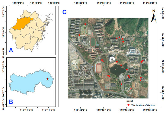
Figure 1.
Study site. Picture (A) is the urban distribution map of Zhejiang Province, China, and the location of Hangzhou City, Zhejiang Province; picture (B) is Lin’an District; picture (C) is the sampling area, and the red dots represent the sampling points, indicating a total of 21 tree species sampling points.
2.2. The Workflow
The experimental process was divided into four steps: (1) Data processing: use mobile terminal equipment to capture images and perform data enhancement on the images while realizing data expansion to generate tree species recognition datasets. (2) Feature extraction: Load the pretrained CNN model, improve the model, and complete the fitting training, using the CNN model for advanced abstract feature extraction. (3) Tree species identification: Bring abstract features into the classifier for training and use the classifier to identify tree species on the unlearned test set. (4) Results analysis: multiple indicators were used to evaluate the performance of the composite model, and the main focus areas of each CNN experimental model were analyzed. The specific experimental flow is shown in Figure 2.
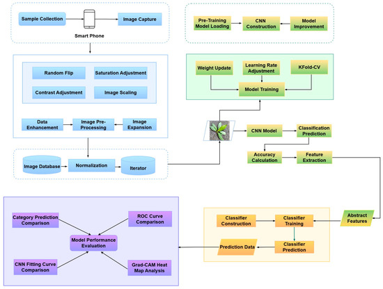
Figure 2.
Experimental flowchart of tree species image recognition based on improved CNN model and classifier.
2.3. Image Acquisition and Processing
The sample trees were mainly focused on street tree species on campus, including local native species. The sample design in the study was different from the traditional image acquisition ideas of previous researchers: the image acquisition was mainly single leaves. The main body of this experiment involved branches with many leaves and twigs, which retain more characteristics of leaf arrangement and twigs growth shape, and at the same time increase the diversity and complexity of the image, which was more in line with the needs of actual application scenarios. As the morphological characteristics of the leaves and branches tend to be perfect in summer, the experimental collection time was concentrated on the first ten days of July, so the appearance of the collected samples was representative to a certain extent, and the samples were collected from a total of 142 sample trees. The shooting equipment used many smart mobile phones of Apple, Huawei, and other brands, and the running memory and hard disk capacities were higher than 3 GB and 64 GB, respectively. Due to the tallness of the sample trees, this study used a high branch shear tool to collect samples, measured the diameter at breast height (DBH) of the sample trees as the difference, and randomly cut branches from around the sample trees, according to different canopies, growth states, and light conditions, and used multi-leaf twigs, which were immediately laid on the asphalt pavement for filming, thereby preserving the background information of the road surface and noise of light and dark changes. At the same time, randomly switched the shooting angles. The captured sample images are shown in Figure 3.
The original image size of 4608 × 3456 pixels was obtained, and the uncompressed original image was divided into training and test sets in a ratio of 80% to 20%. The original image was reduced isometrically using bilinear interpolation. The feature image size was reduced to 658 × 493 pixels. Enhanced and expanded data with random rotation cropping, brightness, and saturation adjustment. The expanded data volume was five times the original data. We scaled the expanded image size to 224 × 224 pixels, then performed vertical, horizontal, random flips, small amplitude random scaling, and normalization operations to complete the secondary data enhancement of the image, enriching the data distribution of the training set, and improving the generalization ability and robustness of the model.

Figure 3.
The leaf sample images of the 21 selected tree species listed in Table 1.

Table 1.
The parameters of the sampled trees. D_Min and D_Max represent the minimum DBH and maximum DBH of all sample trees from these tree species. The last three columns represent the number of original images and the number of training and test samples after data enhancement and expansion.
Table 1.
The parameters of the sampled trees. D_Min and D_Max represent the minimum DBH and maximum DBH of all sample trees from these tree species. The last three columns represent the number of original images and the number of training and test samples after data enhancement and expansion.
| ID | Species | D_Min | D_Max | Original | Train | Test |
|---|---|---|---|---|---|---|
| 1 | Acer buergerianum | 13 | 21.8 | 254 | 1015 | 255 |
| 2 | Albizia julibrissin | 15.5 | 23.4 | 218 | 870 | 220 |
| 3 | Acer palmatum f. atropurpureum | 7 | 9.6 | 242 | 965 | 245 |
| 4 | Castanopsis eyrei | 11.2 | 17 | 252 | 1005 | 255 |
| 5 | Choerospondias axillaris | 12.9 | 24.4 | 219 | 875 | 220 |
| 6 | Cinnamomum camphora | 19.5 | 24.7 | 232 | 925 | 235 |
| 7 | Elaeocarpus glabripetalus | 16.9 | 29.5 | 228 | 910 | 230 |
| 8 | Ginkgo biloba | 19.3 | 27.1 | 220 | 880 | 220 |
| 9 | Ilex chinensis | 18.6 | 23.7 | 229 | 915 | 230 |
| 10 | Ilex integra | 6.7 | 11.5 | 206 | 820 | 210 |
| 11 | Liquidambar formosana | 11.6 | 15.2 | 206 | 820 | 210 |
| 12 | Liriodendron chinense | 21.2 | 29.8 | 224 | 895 | 225 |
| 13 | Magnolia biondii | 17.5 | 24.1 | 254 | 1015 | 255 |
| 14 | Magnolia denudata | 21 | 30 | 223 | 890 | 225 |
| 15 | Michelia chapensis | 22.6 | 27.3 | 286 | 1140 | 290 |
| 16 | Sapindus mukorossi | 14.2 | 24 | 201 | 800 | 205 |
| 17 | Taxodium ascendens | 24.4 | 34.8 | 203 | 810 | 205 |
| 18 | Taxodium distichum | 31.2 | 34.9 | 220 | 880 | 220 |
| 19 | Prunus cerasifera f. atropurpurea | 7 | 9.6 | 222 | 885 | 225 |
| 20 | Koelreuteria bipinnata var. integrifoliola | 12.9 | 24.4 | 211 | 840 | 215 |
| 21 | Cerasus serrulata var. lannesiana | 18.8 | 28.5 | 234 | 935 | 235 |
| Total | 4784 | 19,090 | 4830 | |||
2.4. Optimization Algorithms in CNN
In this study, the CrossEntropyLoss function was chosen as a parameter for model optimization and calculation of gradients. Its basis is the softmax function [22]. The function can be expressed as Equation (1).
where xk denotes the predicted value of the k label, and N is the total number of label categories. Additionally, the e function normalizes the predicted value of the corresponding category to between (0 and 1), and the softmax output results in the predicted probability of the category.
The CrossEntropyLoss function formula is defined as Equation (2) [23]:
where is the real label and is the predicted value of the real label. Softmax function, which calculates the predicted probability of , where ∈ [0, 1], the closer the output of softmax() is to 1, the closer the output of is to 0.
The LeakyReLU activation function is added to the model in the SE-ResNet50 and MixNet XL models [24]. Unlike the ReLU function [25], which sets all negative values to zero, this activation function retains negative information, regulates the zero-gradient problem of the negative values, and expands the range of the ReLU function, which is defined as Equation (3) [25].
where denotes the weight, i.e., the reduction ratio corresponding to negative numbers, and the parameter is set to 0.01.
The EfficientNet B2 model differs from other models in that it uses SiLU as the activation function, and SiLU has continuous, smooth, and non-monotonic properties that offer significant advantages in deep neural networks, the calculation formula is as Equation (4) [26]:
In the experiments, the K-Fold–CV method is used to train the recognition ability of the model, which is different from the common model training method that divides the training dataset into a training dataset and validation dataset. It can effectively prevent the overfitting of the training set and cope with the problem of poor generalization ability caused by the insufficient amount of data. The model training sets the parameter k = 5, and each k subset is used as the validation set and the remaining k − 1 subsets as the training set [28]. The validation set is independent of the learned training set, and its accuracy and error provide a good validation of the model’s ability to generalize to both the training and test sets. Each divided training set has different feature distributions and using k models to extract features can balance the way of feature extraction under different feature distributions and increase the generalization ability of the model [29]. The hardware and software environment configurations for dataset construction, model fitting, and testing are shown in Table 2.
Table 2.
Hardware and software environments.
2.5. The Descriptions of Classifiers
In this study, the SVM classifier was used in combination with the SE-ResNet50 model. The SVM classifier uses a small number of key samples as support vectors, i.e., the sample points closest to the hyperplane, to construct the hyperplane and distinguish the sample classes. It also maximizes the distance between the hyperplane, reduces the interference of the samples to the model, increases the robustness of the model, and reduces the model error [30,31].
The KNN algorithm was used as a classifier to learn the key features extracted by the MixNet XL model. The KNN algorithm is one of the supervised learning methods that use the Euclidean distance algorithm to calculate the distance between the dataset samples and the predicted samples and incrementally rank them [32]. The nearest sample point to the prediction sample was found. The number of categories of k samples was counted and the majority voting method was used to decide the prediction sample categories [33,34].
RF was used as a classifier for the feature extractor of the EfficientNet B2 model. RF builds datasets for multiple decision trees in a random and playback manner so that each tree gets a different distribution of training data and uses feature random sampling to randomly select some features for decision training [35]. The decision trees obtained by combining the different distributions of samples and features are diverse, and the predictions of the combined multiple decision trees present the final prediction results and improve the generalization ability and robustness of the model to new sample predictions [36].
2.6. Convolutional Neural Network
In this study, we used migration learning to initialize the model when training the convolutional neural network. Transferring the knowledge learned in different domains to the new task through transfer learning can improve the model performance [37,38]. We use a pretrained network to apply the knowledge learned from the ImageNet dataset training to a new task, i.e., the tree species recognition task [39], to improve the initial learning ability of the model, to fine-tune the parameters of the model to achieve the desired recognition effect during the learning process of the new task, and to improve the model structure to increase the final tree species recognition accuracy of the model [40].
There are many CNN models. In this study, we chose the SE-ResNet50, MixNet XL, and EfficientNet B2 models to extract the leaf features. The SE-ResNet50 model adds the Squeeze-and-Excitation (SE) attention module, applies the learned channel weights to the original features to represent the relevance of the channel features to the key information, enhances the importance of the key channel features, and suppresses the channel features with the lesser role [41]. Combined with the jump link of the residual module to cope with the degradation problem of gradient disappearance arising from continuing learning after the accuracy reaches saturation as the depth of the model increases, the mapping of input information to output retains the integrity of information, reduces the difficulty of optimizing residual mapping, and achieves high recognition accuracy, even when the depth of the model increases [42]. The output dimension is changed by convolutional layer operations to ensure that the original input x is summed with F(x) calculated through a series of convolutional layers [43], activation layers, etc., to yield H(x), i.e., the residual result, The residual equation is as Equation (6).
Using the lightweight MixNet XL model instead of a single-sized convolution kernel to compute the features of all the channels in the convolution layer operation, multiple channels are grouped and brought into different-sized convolution kernels for convolution computation, while local perceptual fields of different sizes are used to obtain high-level abstract features. It changes the operational limitation of normal convolution kernels, which is the degradation of accuracy in later stages due to the large size of convolution kernels. The use of mixed depth-separated convolution (MixConv) allows the use of convolution kernels of different sizes to achieve a balance between computational workload and high resolution and effectively reduce computational effort [44].
The upper part of Figure 4 represents the normal convolution operation, where all channel features use the same height and width convolution kernels and kin. Figure 4 indicates the scale of the convolution kernel. The lower part of Figure 4 is divided into mixed convolution kernel computation flow, where groups are combinations of multiple channels and each group uses a different size of convolution kernel, and Concat connects the feature maps output from different groups as the input features of the upper layer.
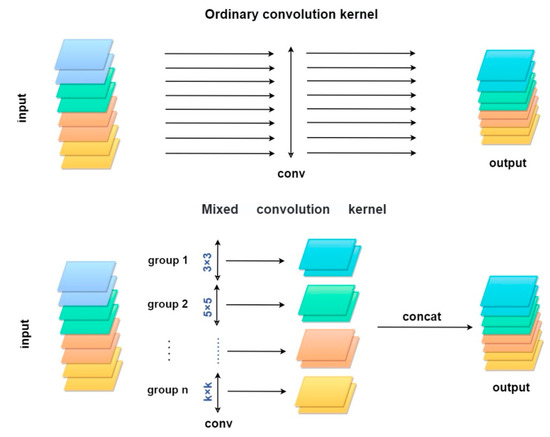
Figure 4.
Ordinary and mixed convolution kernel comparison.
The EfficientNet B2 model was designed based on the MBConv module and used balanced composite coefficients to scale the model to get the improvement of accuracy and efficiency [17]. The composite coefficients include w, d, and r. Here, w is the number of channels and increasing w makes the model training easier; d is the depth of the model and higher d values indicate more complex and diverse acquired features; r is the resolution size and the larger r values denote higher image resolutions.
2.7. Model Framework
The three CNN networks (SE-ResNet50, MixNet XL, and EfficientNet B2) were combined with classical classifiers KNN, SVM, and RF. The hyperparameter settings used to build all CNN models are shown in Table 3, where the learning rate of the VGG16 model is 1 × 10⁻⁴. The SE-ResNet50 model was combined with a residual network and attention mechanism and SVM was used to distinguish sample categories by classification hyperplane. MixNet XL models use mixed convolution kernels to extract abstract features with different resolutions and concatenate them to solve the accuracy optimization problem caused by the increase in the convolution kernel size. Finally, the KNN algorithm calculates the distance between the samples by Euclidean distance, and then, the tree species distribution of the nearest K samples was calculated, and the majority voting method was used for the predictions. EfficientNet B2 improves the accuracy and speed by tuning and balancing the depth, width, and resolution of the model. EfficientNet B2 combines random forest (RF) to integrate multiple decision trees, and some features are randomly selected for training after multiple training sets are formed [45]. The RF design simplifies data interdependence and enhances model generalization.
Table 3.
Model hyperparameter settings.
For the EfficientNet B2 model, the BatchNorm layer, Dropout layer, and fully connected layer (FC) were added after removing the final classification module. In the MixNet XL and SE-ResNet50 models, the last fully connected layer was removed and changed to the LeakReLU layer, Dropout layer, and fully connected layer. At the end of the training, the last fully connected layer of all models was removed and used as a feature extractor. The extracted high-level abstract features were brought into the classifier for training and testing to complete the final recognition task.
MixNet XL used KNN (nearest neighbors) classifier; EfficientNet B2 used RF (random forest) classifier; SE-Resnet50 used an SVM classifier. The composite model framework of CNN combined with each classifier is shown in Figure 5.
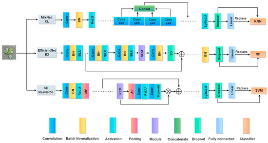
Figure 5.
Composite framework for CNNs and classifiers. MP and AP denote the maximum and average pooling layers, respectively, and SEM and REM denote SE Attention Module and Residual Module, respectively. SD denotes Stochastic Depth, and LyReLU denotes the activation layer based on the LeakyReLU algorithm.
2.8. Accuracy Evaluation Metrics
Four commonly used metrics including overall accuracy (OA), precision, recall, and F1-score were selected to evaluate the training algorithms and model predictive capability [46]. The F1-score considers both the accuracy and recall of the prediction results and is a reconciled average of the accuracy and recall. The four categories of parameters used in the calculation are true positives (TP), false positives (FP), true negatives (TN), and false negatives (FN) [47]. In the experiment, the macro average method was used to calculate the mean value of a single category index as the overall index of the model. The specific calculations of the above indicators are represented in Equations (7)–(11).
where is the corresponding category and is the total number of categories.
Overall accuracy (OA) represents the ratio of the number of correctly predicted samples to the total number of predicted samples. Macro_Precison represents the ratio of correctly predicted positive sample numbers to the total predicted positive sample numbers. Macro_Recall represents the ratio of correctly predicted positive sample numbers to the true positive total sample numbers. The Macro_F1 is a combined indication for Macro_Precison and Macro_ Recall, which is an overall index for the performance evaluation. Macro indicates that the indicator is the average of all categories of indicators.
The receiver operating characteristic (ROC) curve was used as one of the performance indicators simultaneously for evaluating the performance of the model, and the area covered by the ROC curve was calculated, resulting in the AUC value. The ROC curve had two parameters: (1) The true-positive rate (TPR), which was equivalent to the recall indicator that is the proportion of positive samples correctly classified as positive among all the positive samples [48,49]. (2) The false-positive rate (FPR), which was the proportion of all negative samples that are incorrectly classified as positive. The macro-average method was used to calculate the AUC value. The TPR index was directly proportional to the model performance, whereas the FPR index was inversely proportional to the model performance. That is, the closer the ROC curve is to the upper left corner, the higher the AUC value and the better the performance of the model. The specific calculation of FPR is presented in Equation (12).
The AUC calculation method was in the positive and negative sample pairs, the predicted probability of the positive sample was higher than the ratio of the predicted probability of the negative sample. The AUC calculation formula is shown by Equation (13).
where M and N represent the number of positive samples and negative samples, respectively. and represent the predicted probability of positive samples and the predicted probability of negative samples, respectively.
2.9. The Heatmap for Attention Region
To show more clearly the degree of association between different pairs of regions of the input image and the predicted categories, a gradient-weighted class activation map (Grad-CAM) was used in the experiments to draw the heatmap, which is more general than the CAM, without modifying and retraining the network structure [50]. The heatmap was observed to analyze the main image regions that the model focuses on when predicting the categories. The gradient information was obtained by back-propagation calculations of the output from the last convolution layer with the predicted values of class c. Moreover, the gradient information of each channel concerning the predicted value of category c was averaged to indicate the importance of that channel to the prediction of category c, i.e., the weight. The weight calculation formula of each channel is as Equation (14) [51].
where denotes the th channel and denotes the width and height, i.e., pixel values. is the predicted value of category c, and Z is the width × height. is the value of pixels in the channel.
The average value of the predicted value of class c and the gradient information of each element of the k channel is the weight of the k channel. The weight of each channel was weighted and summed with the corresponding channel value of the final convolutional layer output, and the ReLU function was used to calculate the Grad-CAM. The specific calculation formula of Grad-CAM is shown by Equation (15).
where represents the weight of class c predicted values and class k channels, and is the k channel value output by the final convolutional layer.
3. Results
3.1. The Accuracy Evaluation Based on Confusion Matrix
Figure 6 shows the three composite models and the confusion matrix for prediction on the test set using the majority voting method. Among them, the highest recognition error was the prediction of Sapindus mukorossi as Choerospondias axillaris, accounting for 2.4% of the total number of Sapindus mukorossi, with a total of 20 errors for the 4 confusion matrices. Next, Ilex chinensis was predicted as Ilex integra (both belong to the genus Ilex), with a cumulative total of 9 errors across the 4 confusion matrices. SE-ResNet50 combined with the SVM classifier incorrectly predicted Choerospondias axillaris as Koelreuteria bipinnata var. integrifoliolaf four times. The above three types of prediction errors accounted for 50%, 22.5%, and 10% of the total errors of the four confusion matrices, respectively. MixNet XL model combined with KNN classifier and majority voting produced the highest prediction results with the same total recognition accuracy of 99.86%. The classification result of the majority vote was composed of the prediction results of the three composite models, meaning the classification error was concentrated on the above two main classification errors. MixNet XL combined with RF confused the otherwise incorrect classification results.
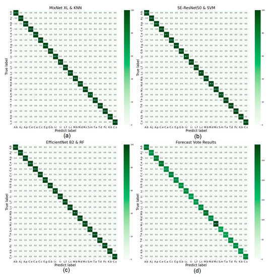
Figure 6.
The accuracy evaluation confusion matrix for the three models. ((a): MixNet XL and KNN; (b): SE-ResNet50 and SVM; (c): EfficientNet B2 and RF) and the majority voting method (d). The x-axis is the predicted tree species labels, the y-axis is the actual tree species labels, and the number along the diagonal is the accuracy of each corresponding tree species. The tree species category order in the figure corresponds to Table 1.
Figure 7 shows the two tree species with the highest frequency of misclassification. The leaves of both Sapindus mukorossi and Choerospondias axillaris have an opposite arrangement pattern, and the profiles of the leaf veins and leaf edge are also similar. These resulted in highly similar leaf traits. Similarly, the Ilex chinensis and Ilex integra tree species belong to the same genus, and the leaf arrangement pattern, veins, shapes, and edges are quite similar. The major difference was in the leaf top shapes. The Ilex chinensis has an acerate top, while the Ilex integra has a relatively round top, which is the major leaf trait that helps differentiate these two species with fewer errors than the Sapindus mukorossi and Choerospondias axillaris species.
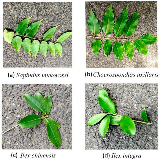
Figure 7.
The two pairs of twigs and leaves images with the highest misclassification frequency.
3.2. Accuracy Evaluation for Tree Species Using F1-Score
Using the F1-score as an evaluation index, we compared the difference in predictive ability between composite and original models for each tree species. The F1-score for most tree species based on the composite models was greater than those based on the original models. The F1-score for the composite models ranged from 0.978 to 1.0, while the original models ranged from 0.858 to 1.0. The lowest F1-score based on the composite models occurred for Sapindus mukorossi (0.978), followed by Choerospondias axillaris (0.982). As inferred from Figure 8, the lowest F1-score for Sapindus mukorossi was because it can be easily misinterpreted as Choerospondias axillaris, while the Choerospondias axillaris can be easily misinterpreted as Koelreuteria bipinnata var. integrifoliola. In contrast, the lowest F1-score based on the original models occurred for Magnolia biondii (0.858), followed by Ilex chinensis (0.894). Magnolia biondii can be easily misinterpreted as Ilex chinensis or Ilex integra.
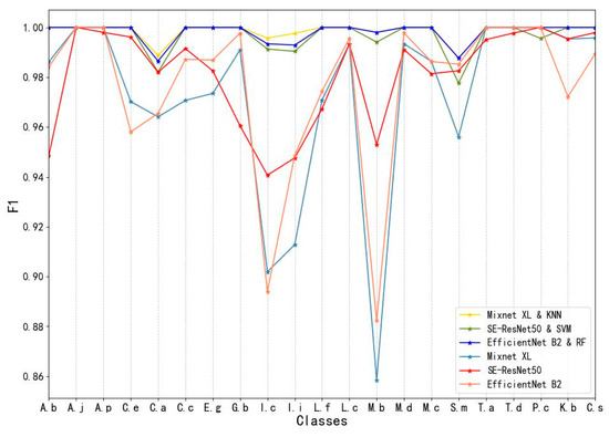
Figure 8.
F1-scores of different tree species based on the composite model and the original model.
Considering that F1-score is the harmonic mean of recall and precision, the composite models show a double improvement of precision and recall metrics, which enhanced the sensitivity of the model to positive samples and reduced the generation of high-frequency misclassification cases for some tree species.
3.3. Convolutional Layer Output Analysis
Figure 9 shows the output abstract feature maps of the first mixed convolution module and the first three convolution layers of the MixNet XL experimental model. The mixed convolution module, which divides the feature maps with the input channel number of 40 into 2 groups, is brought into the convolution kernel with different feature extraction laws for convolution calculation. Furthermore, the obtained feature maps are concatenated and brought into the upper layer for computation. In the first convolutional layer in the abstract feature extraction process, the weight values on the leaf edge, leaf brightness, and darkness are assigned larger, mainly focusing on the leaf contour and leaf brightness for feature extraction and enhancement. The weight values of the partial convolution kernels in the second convolution layer are assigned too small, and the remaining convolution kernels are more concerned with the background texture of the image. The convolution kernel of the third convolutional layer is similar to the feature extraction pattern of the second convolutional layer, with a more uniform distribution of weight values and a focus on the background granular information of the image.
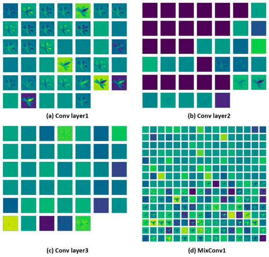
Figure 9.
MixNet XL feature map output.
Since the mixed convolution module used two groups of convolution kernels with different computational rules to extract the features, the feature distribution of the output abstract feature map was different. The first set of mixed convolution kernels in the convolution module focused on the extraction of background texture and leaf contour information, and the second set of mixed convolution kernels focused on the leaf light and shade changes, and leaf contour information.
With the further calculation of convolutional layers, the number of channels increases, with the scales of the output feature map decreasing, and the focus of feature extraction becomes more diversified. Therefore, Figure 9d shows that the hybrid convolution kernel used receptive fields of different scales to extract features with different emphases without adding additional calculations. The resulting abstract feature maps have richer semantics, which can balance calculated amounts while improving accuracy.
3.4. ROC Index Evaluation
Figure 10 shows the ROC curve and AUC area predicted by the generic model, the original model, and the composite model. The ROC curves of MixNet XL combined with KNN and EfficientNet B2 combined with RF are closest to the upper left corner, meaning they have the strongest sensitivity to the positive samples, and the models showed stronger generalization and prediction capabilities. The second was SE-ResNet50 combined with SVM. Compared to the original model, the AUC areas of the above three types of composite models increased by 0.013, 0.011, and 0.008, respectively, and increased by 0.02–0.05 compared to the generic model. Therefore, the composite model exhibited the best predictive performance. In contrast, the VGG16 model curve was closest to the diagonal and had the lowest AUC value. Therefore, the classification and ranking ability and prediction effect of the composite model proposed in this study were improved compared to the original model.
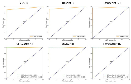
Figure 10.
ROC curves in each model.
Figure 11 shows the prediction accuracy learning curves for all the models in the test set. The experimental model curves were generally higher than the other models, and the initial learning accuracy was higher than the other models, indicating that the initial weight assignment was more accurate in the sample learning process, and all experimental models converged to the fitted state in accuracy at epoch = 13. VGG16 had the lowest accuracy of 0.903, and the initial learning accuracy was also lower than the other models. Compared to the other models, the accuracy of the experimental model was increased by 1.4% to 9.2%; thus, obtaining a better recognition accuracy for the same recognition task and achieving the fitted state with fewer iterations.
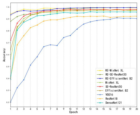
Figure 11.
Accuracy of all models on the test set; RE indicates the experimental model.
3.5. Evaluation of Different Model Metrics
We further calculated the evaluation metrics, including over accuracy, precision, recall, F1-score, and AUC, to compare the predictive results for each model, and the specific values are shown in Table 4. The MixNet XL model with the KNN classifier had the highest recognition accuracy in all four metrics, followed by the EfficientNet B2 model with RF classifier, which was followed by the SE-ResNet50 model combined with the SVM classifier. Compared to VGG16, ResNet18, and DenseNet121, MixNet XL combined with KNN had increased accuracy, precision, recall, F1-score, and AUC area by 4.1%–9.57%, 3.73%–8.51%, 4.07%–9.64%, 4.02%–9.73%, and 0.021–0.05, respectively.
Table 4.
Model metric comparisons. F1-score indicator values converted to percentage display.
Compared to the original models: the MixNet XL, SE ResNet 50, and EfficientNet B2 models, the overall accuracy of the composite model was increased by 2.63%, 1.55%, and 2.21%, respectively, while the F1-score increased by 2.16%–8.53%, and the AUC increased by 0.008–0.013; moreover, the recall and precision increased significantly, by approximately 2%–10%. Based on the above metrics, the composite model showed improvements in overall accuracy, precision, recall, F1-score, and AUC compared to the generic and original models, with an overall accuracy improvement of 1.55%–9.57%.
3.6. F1-Score and Loss Curve
Figure 12 shows the change curves in the F1-scores and loss values of the original model and experimental models as the number of training iterations increased. The F1-score and loss values of the experimental models were the average values of the corresponding metrics of the K-Fold–CV models. The initial F1-score of the experimental models was higher than the original models. The initial F1-score of the RE-SE-ResNet50 model was slightly lower than the other experimental models, yet as the iteration numbers increased, they increased to over 0.97 at epoch = 20, which is an improvement of 2.2%–3.6% compared to the original models.
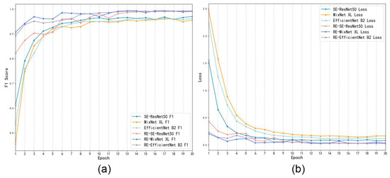
Figure 12.
The curves for F1-score and loss values for the original model and the experimental models. Picture (a,b), respectively, show the curve changes for F1-score and loss of the original and experimental models with the increase of epochs.
The initial losses of the experimental models were all lower than the original models. The initial losses of the RE-SE-ResNet50 model were greater than the other two experimental models, although the losses gradually decreased as the iterations increased, and they were 1.124–2.041 lower than the original models at epoch = 20. The losses were all lower than 0.032 for all experimental models, and the losses were 0.054–0.14 lower than the original models. The experimental models tended to fit without significant fluctuations at epoch = 13, and the classification results were better than the original models. Therefore, the experimental models can achieve better recognition capability with the same number of training times. It can be seen that the improved experimental model can obtain better feature extraction performance and provide high-level abstract features for classifier training and prediction.
3.7. The Main Attention Regions for Different Recognition Models
To illustrate the important regions of concern in the prediction of different models, we applied the Gradient-weighted Class Activation Mapping (Grad-CAM) method to generate the heatmap. Figure 13 indicated that the attention regions of MixNet XL and EfficientNet B2 models in the final convolutional layer were mixed with different background features, especially in the MixNet XL K-FOLD1 model, the activation regions near the twigs background were especially obvious (Figure 12). MixNet XL model had a larger activation area, which focused on the front and middle positions of multiple leaves; thus, had a larger range of recognition attention regions. Except for the K-FOLD3 model, other models in the SE-ResNet50 model could better concentrate on the twigs and dense-leaf region and had no dispersion in the attention region. The key activation area gradually decreased from the branches and leaves to the front of the leaves.
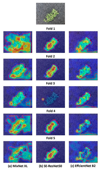
Figure 13.
Multiple K-Fold models acquire heatmaps of attention regions. Heatmaps were generated based on the Grad-CAM method.
The main attention regions in the EfficientNet B2 model were located in the leaf positions at the smaller regions, thereby mixed with the small background regions. The key activation regions (red and orange regions) of the EfficientNet B2 model were smaller and more dispersed than the other models. Therefore, EfficientNet B2 performed main feature extraction and weight distribution for small-scale areas. The feature output in the final convolutional layer of the SE-ResNet50 model performed best in locating the main regions of interest for recognizing objects, and the focus regions were more concentrated. In contrast, the main attention area of the MixNet XL model was concentrated in the region of the dense leaves, and the attention area was more dispersed and mixed with some background features.
In the three models, the weight distribution of each channel of SE-ResNet50 was more in line with the data distribution law, and the positioning of the important areas was more accurate.
4. Discussion
Our proposed method needs less equipment to collect the leaf images and also does not need to apply complicated and multiple preprocessing jobs compared to classifications based on satellite images and other tree features, such as wood and barks [21,52]. The leaf image collection in this study only required the use of high branch shears to collect leaves and smartphones to capture the leaf images. Compared to the previous samples using wood texture and single leaves as the main feature information [53,54], the samples used in this experiment were multiple twigs and multiple leaves, which makes the model fitting more challenging and discerning. In addition, our method was not affected by common natural interferences, such as location, viewing angles, and light conditions. Thus, our method is more appropriate for applications in complex conditions, such as the field survey for forest resources. Our proposed method can be integrated into plenty of mobile terminal applications for tree species recognition and can improve recognition accuracy.
Many previous studies have used traditional classifiers to predict tree species classes, which require complex data preprocessing and feature extraction work, such as computing a histogram of gradients (HOG) [10], computing grayscale co-generation matrix (GLCM) descriptors, and texture descriptors to represent important features of images [55]. In this study, we use CNNs instead of the traditional feature extraction step, thereby reducing the workload involved in image preprocessing and feature extraction.
We used the classifiers as the final decision model to predict the tree species according to the extracted features by the CNNs. Our method replaced the CNN fully connected layer for prediction and increased the predictive performance of the model. Compared to the original models: MixNet XL, SE-ResNet50, and EfficientNet B2, the overall accuracy was experimental by 2.63%, 1.55%, and 2.21%, respectively. The accuracies of all three composite models were higher than the recognition accuracies in previous studies [10,11,19], proving the effectiveness of the experimental method.
The experimental accuracy in this study was due to three reasons. Firstly, the current CNN model, which possesses better performance, was used as the feature extractor, alongside the pretrained model. Secondly, the K-Fold–CV method was used for model training and validation to improve the robustness and generalization of the model and to unify the feature distribution of the training set. In addition, the classifier was used for tree species identification instead of the traditional fully connected layer. The error in prediction was mainly caused by the relatively higher misclassification rates between Sapindus mukorossi and Choerospondias axillaris, and between Ilex chinensis and Ilex integra, due to their high interspecific similarity in leaf shape, leaf arrangement order, and vein texture.
In this experiment, the automatic identification of tree species images acquired by mobile devices was completed by constructing a composite model. Remote sensing-based methods enable image sampling and forest surveys in areas with complex topography. Many researchers have tried to apply remote sensing technology to forestry tree species identification and resource inventory. Large-area images can be obtained at one time by using satellite remote sensing, which is suitable for large-scale tree species identification. In the study of applying the CNN model to remote sensing data processing, Huang et al., 2023 [56] used the DJI Phantom 4 UAV to obtain a total of 1247 forest remote sensing images as source data for tree species identification. Furthermore, using MobileNetV2 as the backbone network for feature extraction, a dual-attention residual network (AMDNet) was proposed, which achieved an accuracy of 93.8% on mIoU (mean intersection over union). The improved CNN model in this experiment can continue to be applied to the feature extraction of large-scale remote sensing images to assist in the completion of large-scale tree species identification tasks. Combining remote sensing technology with deep learning technology will be one of the powerful ways to improve the traditional large-scale forest condition survey and forest tree species mapping [15,57].
5. Conclusions
We used the MixNet XL model with mixed convolutional kernels, which uses convolutional kernels of different scales to extract features with different resolutions, improving the problem of difficulty to optimize accuracy due to the expansion of convolutional kernels. The SE-ResNet50 model uses the attention mechanism combined with the residual module to increase the weights of key features and retain the learning information to improve the gradient disappearance problem caused by the increase in depth. The EfficientNet B2 model modifies the number of channels of the model, the depth of the model, and the resolution size of the input features by balancing the composite coefficients to achieve optimization of the model structure and accuracy improvement. Further, the three model structures are fine-tuned to accelerate the model fitting rate through LeakyReLU, Dropout, and BatchNorm layers to prevent the overfitting phenomenon and increase the model generalization ability.
The model was trained and validated by combining the K-Fold–CV methods to balance the feature distribution of the training set and prevent overfitting. The fully connected layers of the experimental model were replaced with KNN, SVM, and RF classifiers to perform category predictions. Grad-CAM heatmaps show important activation areas and emphasize the different experimental models. Among them, the activation area positioning ability of the SE-ResNet50 model was the best, except for the K-Fold3 model.
The overall accuracy of the composite models was higher than the other models. There was a 1.76%–9.57% improvement in accuracy. The recognition errors mainly occurred between Sapindus mukorossi and Choerospondias axillaris, and between Ilex chinensis and Ilex integra. After observing the images, we found that the growth distribution, shape, and texture of the leaves had a high similarity, which caused a lot of recognition errors.
This study performed image recognition based on 21 classes of tree species with 99.86% recognition accuracy by improving the MixNet XL, SE-ResNet50, and EfficientNet B2 models combined with KNN, SVM, and RF classifiers. The images in the dataset mainly show the characteristics of multiple twigs and multiple leaves, which is more in line with the growth characteristics of trees, meaning that the application range of the model is wider. It can provide important information for forest resource inventory, urban tree species configuration planning and design, and the conservation of rare and endangered tree species. At the same time, the research on automatic recognition of tree species images also provides technical support and innovative ideas for the intelligent development of forestry. This experiment uses CNN models as a feature extractor to achieve automated high-level abstract feature extraction while reducing the workload. Moreover, combining the models with the classifiers as a decision model, improved the overall classification accuracy and provided a new modeling idea for the development of related software.
Comparing the fitting accuracy of each CNN model can promote the framework structures of the MixNet XL and EfficientNet B2 models to become more suitable for advanced feature extraction of multi-leaf and multi-twig samples, and the extracted abstract feature distribution became more suitable for this type of recognition task.
Van Horn et al., 2018 developed the iNaturalist application based on the multi-feature recognition of leaves, flowers, bark, etc., and its recognition accuracy was 67% due to the impact of category balance [58]. Compared to the former, the number of tree species in this study was small; however, the accuracy rate was greatly improved due to the use of a composite model architecture and a more balanced category distribution.
In previous studies, a single CNN model was usually used as a tree species identification model [3], yet in this study, a CNN model was used as a feature extractor combined with a machine learning algorithm as a decision maker to form a composite model. Its design will help CNN models be used with different feature extraction preferences for feature extraction and information fusion of different arbor organs, such as leaves and branches, thereby improving the recognition accuracy and providing new technical support and innovative ideas for future research.
In order to better handle complex recognition tasks, we need to expand the number of tree species in the dataset for future research, while increasing the recognition of features such as bark and flowers. In future application scenarios based on multi-feature recognition and background noise, in order to ensure the accuracy of recognition, features such as bark and leaves can be fused, and the final prediction can also be made using the majority voting method. We need to continuously improve the network structure of the model to ensure recognition accuracy and training efficiency. We also plan to integrate the composite model into the mobile terminal to complete the research and development of the tree species identification APP.
Author Contributions
X.S. is responsible for data collection, resource integration, experiment design, result validation, and writing manuscript; Y.S. is responsible for situation analysis, field investigation, and project management; L.X. and Y.Z. are responsible for supervision and editing. All authors have read and agreed to the published version of the manuscript.
Funding
This research was funded by the Key Research and Development Program of Zhejiang Province (Grant number: 2023C02003); the National Natural Science Foundation of China (Grant number: 32001315; U1809208; 31870618); and the Scientific Research Development Fund of Zhejiang A&F University (Grant number: 2020FR008).
Data Availability Statement
The data presented in this study are available on request from the corresponding author. The data are not publicly available due to the confidentiality of the projects.
Conflicts of Interest
The authors declare no conflict of interest.
References
- Wäldchen, J.; Rzanny, M.; Seeland, M.; Mäder, P. Automated Plant Species Identification—Trends and Future Directions. PLoS Comput. Biol. 2018, 14, e1005993. [Google Scholar] [CrossRef] [PubMed]
- Barré, P.; Stöver, B.C.; Müller, K.F.; Steinhage, V. LeafNet: A Computer Vision System for Automatic Plant Species Identification. Ecol. Inform. 2017, 40, 50–56. [Google Scholar] [CrossRef]
- Carpentier, M.; Giguere, P.; Gaudreault, J. Tree Species Identification from Bark Images Using Convolutional Neural Networks. In Proceedings of the 2018 IEEE/RSJ International Conference on Intelligent Robots and Systems (IROS), Madrid, Spain, 1–5 October 2018; IEEE: New York, NY, USA, 2018; pp. 1075–1081. [Google Scholar]
- Gogul, I.; Kumar, V.S. Flower Species Recognition System Using Convolution Neural Networks and Transfer Learning. In Proceedings of the 2017 Fourth International Conference on Signal Processing, Communication and Networking (ICSCN), Chennai, India, 16–18 March 2017; IEEE: New York, NY, USA, 2017; pp. 1–6. [Google Scholar]
- Zhao, Z.-Q.; Ma, L.-H.; Cheung, Y.; Wu, X.; Tang, Y.; Chen, C.L.P. ApLeaf: An Efficient Android-Based Plant Leaf Identification System. Neurocomputing 2015, 151, 1112–1119. [Google Scholar] [CrossRef]
- Somers, B.; Asner, G.P. Tree Species Mapping in Tropical Forests Using Multi-Temporal Imaging Spectroscopy: Wavelength Adaptive Spectral Mixture Analysis. Int. J. Appl. Earth Obs. Geoinf. 2014, 31, 57–66. [Google Scholar] [CrossRef]
- Lee, J.; Cai, X.; Lellmann, J.; Dalponte, M.; Malhi, Y.; Butt, N.; Morecroft, M.; Schönlieb, C.-B.; Coomes, D.A. Individual Tree Species Classification from Airborne Multisensor Imagery Using Robust PCA. IEEE J. Sel. Top. Appl. Earth Obs. Remote Sens. 2016, 9, 2554–2567. [Google Scholar] [CrossRef]
- Fassnacht, F.E.; Latifi, H.; Stereńczak, K.; Modzelewska, A.; Lefsky, M.; Waser, L.T.; Straub, C.; Ghosh, A. Review of Studies on Tree Species Classification from Remotely Sensed Data. Remote Sens. Environ. 2016, 186, 64–87. [Google Scholar] [CrossRef]
- Wäldchen, J.; Mäder, P. Plant Species Identification Using Computer Vision Techniques: A Systematic Literature Review. Arch. Comput. Methods Eng. 2018, 25, 507–543. [Google Scholar] [CrossRef]
- Sugiarto, B.; Prakasa, E.; Wardoyo, R.; Damayanti, R.; Dewi, L.M.; Pardede, H.F.; Rianto, Y. Wood Identification Based on Histogram of Oriented Gradient (HOG) Feature and Support Vector Machine (SVM) Classifier. In Proceedings of the 2017 2nd International conferences on Information Technology, Information Systems and Electrical Engineering (ICITISEE), Yogyakarta, Indonesia, 1–3 November 2017; IEEE: New York, NY, USA, 2017; pp. 337–341. [Google Scholar]
- Iwata, T.; Saitoh, T. Tree Recognition Based on Leaf Images. In Proceedings of the The SICE Annual Conference 2013, Nagoya, Japan, 14–17 September 2013; IEEE: New York, NY, USA, 2013; pp. 2489–2494. [Google Scholar]
- Lim, K.; Treitz, P.; Wulder, M.; St-Onge, B.; Flood, M. LiDAR Remote Sensing of Forest Structure. Prog. Phys. Geogr. 2003, 27, 88–106. [Google Scholar] [CrossRef]
- Alzubaidi, L.; Zhang, J.; Humaidi, A.J.; Al-Dujaili, A.; Duan, Y.; Al-Shamma, O.; Santamaría, J.; Fadhel, M.A.; Al-Amidie, M.; Farhan, L. Review of Deep Learning: Concepts, CNN Architectures, Challenges, Applications, Future Directions. J. Big Data 2021, 8, 1–74. [Google Scholar] [CrossRef]
- Young, T.; Hazarika, D.; Poria, S.; Cambria, E. Recent Trends in Deep Learning Based Natural Language Processing. IEEE Comput. Intell. Mag. 2018, 13, 55–75. [Google Scholar] [CrossRef]
- Kattenborn, T.; Leitloff, J.; Schiefer, F.; Hinz, S. Review on Convolutional Neural Networks (CNN) in Vegetation Remote Sensing. ISPRS J. Photogramm. Remote Sens. 2021, 173, 24–49. [Google Scholar] [CrossRef]
- Albawi, S.; Mohammed, T.A.; Al-Zawi, S. Understanding of a Convolutional Neural Network. In Proceedings of the 2017 International Conference on Engineering and Technology (ICET), Antalya, Turkey, 21–23 August 2017; IEEE: New York, NY, USA, 2017; pp. 1–6. [Google Scholar]
- Tan, M.; Le, Q. Efficientnet: Rethinking Model Scaling for Convolutional Neural Networks. In Proceedings of the International Conference on Machine Learning, PMLR, Long Beach, CA, USA, 9–15 June 2019; pp. 6105–6114. [Google Scholar]
- Homan, D.; du Preez, J.A. Automated Feature-Specific Tree Species Identification from Natural Images Using Deep Semi-Supervised Learning. Ecol. Inform. 2021, 66, 101475. [Google Scholar] [CrossRef]
- Kim, T.K.; Hong, J.; Ryu, D.; Kim, S.; Byeon, S.Y.; Huh, W.; Kim, K.; Baek, G.H.; Kim, H.S. Identifying and Extracting Bark Key Features of 42 Tree Species Using Convolutional Neural Networks and Class Activation Mapping. Sci. Rep. 2022, 12, 1–13. [Google Scholar] [CrossRef] [PubMed]
- Zhu, M.; Wang, J.; Wang, A.; Ren, H.; Emam, M. Multi-Fusion Approach for Wood Microscopic Images Identification Based on Deep Transfer Learning. Appl. Sci. 2021, 11, 7639. [Google Scholar] [CrossRef]
- Yan, S.; Jing, L.; Wang, H. A New Individual Tree Species Recognition Method Based on a Convolutional Neural Network and High-Spatial Resolution Remote Sensing Imagery. Remote Sens. 2021, 13, 479. [Google Scholar] [CrossRef]
- Jang, E.; Gu, S.; Poole, B. Categorical Reparameterization with Gumbel-Softmax. arXiv 2016, arXiv:1611.01144. [Google Scholar]
- Martinez, M.; Stiefelhagen, R. Taming the Cross Entropy Loss. In Proceedings of the German Conference on Pattern Recognition, Stuttgart, Germany, 10–12 October 2018; Springer: Berlin/Heidelberg, Germany, 2018; pp. 628–637. [Google Scholar]
- Wang, Y.; Yan, J.; Yang, Z.; Zhao, Y.; Liu, T. Optimizing GIS Partial Discharge Pattern Recognition in the Ubiquitous Power Internet of Things Context: A MixNet Deep Learning Model. Int. J. Electr. Power Energy Syst. 2021, 125, 106484. [Google Scholar] [CrossRef]
- Agarap, A.F. Deep Learning Using Rectified Linear Units (Relu). arXiv 2018, arXiv:1803.08375. [Google Scholar]
- Ramachandran, P.; Zoph, B.; Le, Q. V Searching for Activation Functions. arXiv 2017, arXiv:1710.05941. [Google Scholar]
- Chandra, P.; Singh, Y. An Activation Function Adapting Training Algorithm for Sigmoidal Feedforward Networks. Neurocomputing 2004, 61, 429–437. [Google Scholar] [CrossRef]
- Refaeilzadeh, P.; Tang, L.; Liu, H. Cross-Validation. Encycl. Database Syst. 2009, 5, 532–538. [Google Scholar]
- Jung, Y. Multiple Predicting K-Fold Cross-Validation for Model Selection. J. Nonparametr. Stat. 2018, 30, 197–215. [Google Scholar] [CrossRef]
- Abdullah, D.M.; Abdulazeez, A.M. Machine Learning Applications Based on SVM Classification A Review. Qubahan Acad. J. 2021, 1, 81–90. [Google Scholar] [CrossRef]
- Chauhan, V.K.; Dahiya, K.; Sharma, A. Problem Formulations and Solvers in Linear SVM: A Review. Artif. Intell. Rev. 2019, 52, 803–855. [Google Scholar] [CrossRef]
- Peterson, L.E. K-Nearest Neighbor. Scholarpedia 2009, 4, 1883. [Google Scholar] [CrossRef]
- Parvin, H.; Alizadeh, H.; Minaei-Bidgoli, B. Validation Based Modified K-Nearest Neighbor. In Proceedings of the AIP Conference Proceedings, San Francisco, CA, USA, 22–24 October 2008; American Institute of Physics: Melville, NY, USA, 2009; Volume 1127, pp. 153–161. [Google Scholar]
- Guo, G.; Wang, H.; Bell, D.; Bi, Y.; Greer, K. KNN Model-Based Approach in Classification. In Proceedings of the OTM Confederated International Conferences “On the Move to Meaningful Internet Systems”, Sicily, Italy, 3–7 November 2003; Springer: Berlin/Heidelberg, Germany, 2003; pp. 986–996. [Google Scholar]
- Speiser, J.L.; Miller, M.E.; Tooze, J.; Ip, E. A Comparison of Random Forest Variable Selection Methods for Classification Prediction Modeling. Expert Syst. Appl. 2019, 134, 93–101. [Google Scholar] [CrossRef]
- Pal, M. Random Forest Classifier for Remote Sensing Classification. Int. J. Remote Sens. 2005, 26, 217–222. [Google Scholar] [CrossRef]
- Zhuang, F.; Qi, Z.; Duan, K.; Xi, D.; Zhu, Y.; Zhu, H.; Xiong, H.; He, Q. A Comprehensive Survey on Transfer Learning. Proc. IEEE 2020, 109, 43–76. [Google Scholar] [CrossRef]
- Weiss, K.; Khoshgoftaar, T.M.; Wang, D. A Survey of Transfer Learning. J. Big Data 2016, 3, 1–40. [Google Scholar] [CrossRef]
- Feng, H.; Hu, M.; Yang, Y.; Xia, K. Tree Species Recognition Based on Overall Tree Image and Ensemble of Transfer Learning. Trans. Chin. Soc. Agric. Mach. 2019, 8, 235–279. [Google Scholar]
- Lima, E.; Sun, X.; Dong, J.; Wang, H.; Yang, Y.; Liu, L. Learning and Transferring Convolutional Neural Network Knowledge to Ocean Front Recognition. IEEE Geosci. Remote Sens. Lett. 2017, 14, 354–358. [Google Scholar] [CrossRef]
- Hu, J.; Shen, L.; Sun, G. Squeeze-and-Excitation Networks. In Proceedings of the IEEE Conference on Computer Vision and Pattern Recognition, Salt Lake City, UT, USA, 18–23 June 2018; pp. 7132–7141. [Google Scholar]
- He, F.; Liu, T.; Tao, D. Why Resnet Works? Residuals Generalize. IEEE Trans. Neural Netw. Learn. Syst. 2020, 31, 5349–5362. [Google Scholar] [CrossRef] [PubMed]
- Chen, Z.; Xie, Z.; Zhang, W.; Xu, X. ResNet and Model Fusion for Automatic Spoofing Detection. In Proceedings of the Interspeech, Stockholm, Sweden, 20–24 August 2017; pp. 102–106. [Google Scholar]
- Tan, M.; Le, Q. V Mixconv: Mixed Depthwise Convolutional Kernels. arXiv 2019, arXiv:1907.09595. [Google Scholar]
- Oshiro, T.M.; Perez, P.S.; Baranauskas, J.A. How Many Trees in a Random Forest? In Proceedings of the International Workshop on Machine Learning and Data Mining in Pattern Recognition, Berlin, Germany, 13–20 July 2012; Springer: Berlin/Heidelberg, Germany, 2012; pp. 154–168. [Google Scholar]
- Song, Y.; Zheng, S.; Li, L.; Zhang, X.; Zhang, X.; Huang, Z.; Chen, J.; Wang, R.; Zhao, H.; Chong, Y. Deep Learning Enables Accurate Diagnosis of Novel Coronavirus (COVID-19) with CT Images. IEEE/ACM Trans. Comput. Biol. Bioinform. 2021, 18, 2775–2780. [Google Scholar] [CrossRef] [PubMed]
- Glas, A.S.; Lijmer, J.G.; Prins, M.H.; Bonsel, G.J.; Bossuyt, P.M.M. The Diagnostic Odds Ratio: A Single Indicator of Test Performance. J. Clin. Epidemiol. 2003, 56, 1129–1135. [Google Scholar] [CrossRef]
- Davis, J.; Goadrich, M. The Relationship between Precision-Recall and ROC Curves. In Proceedings of the 23rd International Conference on Machine Learning, Pittsburgh, PA, USA, 25 June 2006; pp. 233–240. [Google Scholar]
- Fawcett, T. An Introduction to ROC Analysis. Pattern Recognit. Lett. 2006, 27, 861–874. [Google Scholar] [CrossRef]
- Selvaraju, R.R.; Cogswell, M.; Das, A.; Vedantam, R.; Parikh, D.; Batra, D. Grad-Cam: Visual Explanations from Deep Networks via Gradient-Based Localization. In Proceedings of the IEEE International Conference on Computer Vision, Venice, Italy, 22–29 October 2017; pp. 618–626. [Google Scholar]
- Selvaraju, R.R.; Das, A.; Vedantam, R.; Cogswell, M.; Parikh, D.; Batra, D. Grad-CAM: Why Did You Say That? arXiv 2016, arXiv:1611.07450. [Google Scholar]
- He, J.; Sun, Y.; Yu, C.; Cao, Y.; Zhao, Y.; Du, G. An Improved Wood Recognition Method Based on the One-Class Algorithm. Forests 2022, 13, 1350. [Google Scholar] [CrossRef]
- de Geus, A.R.; Backes, A.R.; Gontijo, A.B.; Albuquerque, G.H.Q.; Souza, J.R. Amazon Wood Species Classification: A Comparison between Deep Learning and Pre-Designed Features. Wood Sci. Technol. 2021, 55, 857–872. [Google Scholar] [CrossRef]
- Yahiaoui, I.; Mzoughi, O.; Boujemaa, N. Leaf Shape Descriptor for Tree Species Identification. In Proceedings of the 2012 IEEE International Conference on Multimedia and Expo, Melbourne, Australia, 9–13 July 2012; IEEE: New York, NY, USA, 2012; pp. 254–259. [Google Scholar]
- Di Ruberto, C.; Putzu, L. A Fast Leaf Recognition Algorithm Based on SVM Classifier and High Dimensional Feature Vector. In Proceedings of the 2014 International Conference on Computer Vision Theory and Applications (VISAPP), Lisbon, Portugal, 5–8 January 2014; IEEE: New York, NY, USA, 2014; Volume 1, pp. 601–609. [Google Scholar]
- Huang, H.; Li, F.; Fan, P.; Chen, M.; Yang, X.; Lu, M.; Sheng, X.; Pu, H.; Zhu, P. AMDNet: A Modern UAV RGB Remote-Sensing Tree Species Image Segmentation Model Based on Dual-Attention Residual and Structure Re-Parameterization. Forests 2023, 14, 549. [Google Scholar] [CrossRef]
- Guo, Q.; Zhang, J.; Guo, S.; Ye, Z.; Deng, H.; Hou, X.; Zhang, H. Urban Tree Classification Based on Object-Oriented Approach and Random Forest Algorithm Using Unmanned Aerial Vehicle (Uav) Multispectral Imagery. Remote Sens. 2022, 14, 3885. [Google Scholar] [CrossRef]
- Van Horn, G.; Mac Aodha, O.; Song, Y.; Cui, Y.; Sun, C.; Shepard, A.; Adam, H.; Perona, P.; Belongie, S. The Inaturalist Species Classification and Detection Dataset. In Proceedings of the IEEE Conference on Computer Vision and Pattern Recognition, Salt Lake City, UT, USA, 18–23 June 2018; pp. 8769–8778. [Google Scholar]
Disclaimer/Publisher’s Note: The statements, opinions and data contained in all publications are solely those of the individual author(s) and contributor(s) and not of MDPI and/or the editor(s). MDPI and/or the editor(s) disclaim responsibility for any injury to people or property resulting from any ideas, methods, instructions or products referred to in the content. |
© 2023 by the authors. Licensee MDPI, Basel, Switzerland. This article is an open access article distributed under the terms and conditions of the Creative Commons Attribution (CC BY) license (https://creativecommons.org/licenses/by/4.0/).