Article

UAV Photogrammetry for Soil Surface Deformation Detection in a Timber Harvesting Area, South Korea

1
Department of Forestry and Environmental Systems, Kangwon National University, Chuncheon 24341, Republic of Korea
2
Division of Forest Science, Kangwon National University, Chuncheon 24341, Republic of Korea
*
Author to whom correspondence should be addressed.
Forests 2023, 14(5), 980; https://doi.org/10.3390/f14050980
Submission received: 29 March 2023 / Revised: 1 May 2023 / Accepted: 6 May 2023 / Published: 10 May 2023
(This article belongs to the Special Issue Forest Harvesting and Forest Product Supply Chain)

Abstract

:
During forest operations, canopy removal results in the soil surface being vulnerable to deformation, negatively impacting soil fertility and water quality. This study utilized unmanned aerial vehicle (UAV) photogrammetry to accurately detect soil surface deformation (SSD). Two-dimensional images were safely collected on a steep slope without real-time kinematics by conducting vertically parallel flights (VPFs). A high-resolution digital surface model (DSM) with a <3 cm resolution was acquired for precise SSD detection. Using DSM of difference (DoD), SSDs were calculated from DSMs acquired in June, July, September, and October 2022. By checking spatial distances at ground control points, errors of DSM alignments were confirmed as only 3 cm, 11.1 cm, and 4 cm from July to June, September to June, and October to June, respectively. From the first month of monitoring, erosion and deposition of approximately 7 cm and 9 cm, respectively, were detected at validation points (VPs). However, from total monitoring, cumulative SSD was assessed as having deposition tendencies at all VPs, even compared to ground truths. Although UAV photogrammetry can detect SSDs, spatial distortion may occur during UAV surveys. For vegetation growth issues, UAV photogrammetry may be unable to capture data on the soil surface itself.

1. Introduction

Forestry is important not only for its wood products but also for its environmental benefits, such as its impact on climate change and water quality and quantity. Forest operations such as clear-cutting cause disturbances in forest soil, primarily due to the use of forest operation machines [1,2,3]. In addition to direct effects such as soil surface deformation (SSD) caused by forest operation machines, forest soils become vulnerable to run-off due to the removal of forest canopies, which protect the soil surface from rainfall energy [4,5,6,7]. Erosion of forest areas negatively impacts forest soils, resulting in decreased soil fertility for reforestation and a reduction in water sources from the conducted operations [8,9,10,11]. Timber harvesting is essential for maintaining modern human life and carbon storage, which mitigates climate change following reforestation [12,13,14]. As human civilization continues to develop, the importance of sustainable forest management will continue to emerge.
Despite human efforts to prevent the negative effects of canopy removal, predicting “where”, “when”, and “how” natural events will occur in these areas remains challenging. Moreover, restoring and preventing SSD in post-canopy removal areas are challenging tasks. Detecting SSD is necessary, given the difficulties in prediction and restoration. However, studies related to the use of unmanned aerial vehicles (UAVs) for SSD detection have focused mainly on large-scale SSDs, such as landslides, and few studies have been conducted on SSD field detection on forest operation sites [15,16].
Recent studies have made significant efforts toward detecting and analyzing SSDs in post-disaster and forest operation areas, despite the difficulties in realistically correlating occurrences to SSDs [17,18,19,20,21,22]. Survey methods utilizing capital-intensive technology, such as remote sensing, UAVs [18], terrestrial light and ranging (LiDAR) systems (TLS) [21], and mobile LiDAR systems [22], have been developed.
Precise SSD detection methods similar to those used in post-forest operations have been utilized in landslide studies. UAV photogrammetry has been proven to be useful in detecting morphologic deformation, and recent 10-year studies have shown that large SSDs, such as landslides, are commonly surveyed using this technique [23,24,25,26,27]. Through UAV surveys, 5 cm class spatial resolution was provided [28], and numerous studies involved landslide surveys with UAV systems and were able to accurately analyze SSDs [18,23]. Despite their high-precision 3D resolution, conducting UAV systems requires site preparation for field reference. Many studies have used ground control points (GCPs) at distinctive objects for reference and measured the coordinates of the corresponding GCPs using a global navigation satellite system (GNSS) [18,29,30]. Surveys from field operations and UAVs using 3D data, such as point cloud data (PCD), were then acquired with the support of the structure from motion (SfM) algorithm. During software processing, SfM detects corresponding points from 2D images collected from UAV surveys, generates a sparse cloud of 3D models, and then densifies the sparse cloud to a dense cloud, which is well known as PCD [31,32].
To achieve the objectives of many studies, such as displacement or deformation detection, in digital elevation models (DEMs) or substitution with digital surface models (DSMs), each acquired time zone must be compared to pre- and post-SSD occurrence data [23,33,34]. This comparison process involves calculating the DSM of the difference (DoD), which requires aligning 3D datasets [35,36,37,38,39]. The alignment of the PCD sets preceded the geo-referencing of 3D data from GCP registration, which were then converted to DSMs. The aligned DSMs were then calculated as DoDs and utilized in SSD analysis and monitoring in most SSD studies [33,39,40].
Previous studies show that methods for detecting SSD have been developed. However, these methods have not yet been applied in post-timber harvesting areas or validated with ground truth (GT) from field surveys. Furthermore, it has not been revealed whether UAV photogrammetry can safely detect forest soils on steep slopes without real-time kinematics (RTKs). Our objectives were to safely detect the SSD on a timber harvesting site using a global positioning system (GPS)-based UAV survey, and determine the precision of the method in detecting SSD by calculating the error by validation. To achieve this, we investigated: (1) the feasibility of detecting SSDs on a timber harvesting area with an open canopy and steep slope using UAV photogrammetry; (2) validation of the detected SSDs by calculating the root mean square error (RMSE) from the GT data from the field survey; and (3) assessment of the total slope deformation monitoring in relation to slope stability and soil erosion.

2. Materials and Methods

2.1. Study Area

This study was conducted on a timber harvesting site in the research forest of Kangwon National University, Gangwon Province, Republic of Korea (37°46′34.4″ N, 127°49′41.1″ E; Figure 1). Timber harvesting was conducted on the study site with a total area of 3 ha in March 2022. The area has a temperate climate with a heavy rainy season in the summer (June–August). During the research period, the monthly precipitation amount averaged 300 mm in the heavy rainy season, and intense rainfall occurred from June to August based on climate features. The site has an average slope of 47%, with altitudes above sea level ranging from 508 m to approximately 628 m. Based on U.S. soil taxonomy, the soil type corresponded to the Mui series (coarse loamy, mixed, Typic Humudepts), and soils in the area consisted of dark brown sandy loam. Logging tracks were generated on the middle and right sides of the study area. From March to June, the surface cover of the area consisted of forest soil, rocks, logging debris, and slightly less vegetation. The steep slopes and high rainfall at the study site create ideal conditions for run-off and SSD [41,42,43].

2.2. UAV Survey

Remote field surveys are necessary to obtain 3D deformation data [44,45,46]. Among the remote-sensing techniques for generating centimeter-class high-resolution 3D data, field surveys using UAV systems are an efficient method in forest areas [44,47,48]. We were able to retrieve a resolution of <3 cm using the UAV photogrammetry method, which provides a cost-efficient surveying system. To properly generate UAV-based 3D data, preprocessing must be performed for site preparation. For geo-reference validation, GCPs were used to apply an accurate coordinate system to the monthly acquired PCDs, and for SSD validation on each monthly acquired PCD, validation points (VPs) were placed in plots.

2.2.1. Preprocess on Study Site

On steep forest slopes, it is near impossible to locate unchanged ground objects. However, the morphological features of tree stumps did not deform in their natural state during the research period without physical interference. Hence, we prepared GCPs with a 40 × 40 cm Fomex texture plate for anti-oxidation and installed them on tree stumps. A total of 29 stumps were selected for GCP installation. During stump selection, the size, surface angle, and location of the stumps were considered for appropriate installation. All the GCPs were fixed on the top of the stumps using screws. Trimble R12i GNSSs were used to acquire coordinate data at the center of the GCPs (Figure 2a).
The GT data collection process is essential for validating SSD in acquired PCDs. For this process, we prepared polyvinyl chloride (PVC) pipes with a 2.6 cm diameter and a length of >50 cm, to which rulers were attached. These PVC pipes were then installed on a total of three plots with characteristics that represented erosion and deposition for GT VPs. The three plots (Plot 1, erosion expected area; Plot 2, wheel track; Plot 3, deposition expected area) were selected for validation of estimated SSD depth from DoD (Figure 2c). GT height was recorded by measuring the relative surface height that appeared on the VP ruler (Figure 2b). However, it was not possible to locate and identify VP pipes in the 3D data, even with a high resolution of <3 cm. For practical applications, the resolution should be acquired at half the size of the object to identify objects using remote-sensing techniques [49]. Thus, instead of identifying the exact features of the VP pipes, a method was conducted to retrieve the location coordinates from the installed pipes. To define the location of the VPs on the 3D data, GNSS equipment was used to acquire the VP coordinates (Figure 2b).

2.2.2. UAV Image Collection

Several trials were conducted to confirm that the VPFs are a reliable high-resolution acquisition method for the study site without RTK. The reconnaissance UAV flights showed that the research site had a steep slope (average of 47%). In surveys with steep slopes, UAV flights have a high risk of crashing when conducted too close to the slope surface. Furthermore, a single flight cannot capture high-resolution 2D images of the lower slope of the study site. Therefore, lower-altitude flights in the monthly UAV surveys were essential under these conditions.
To obtain images for the photogrammetric process, a Da-Jiang Innovations (DJI) Matrice 300 RTK was used as a remote-sensing platform, and a DJI Zenmuse H20T was equipped with a sensor platform. Each platform and sensor weighed approximately 7 kg and 0.82 kg, respectively. Considering the trees on the site slope and the forest located on the sides of the slope, an automatic flight was performed to collect UAV images. To collect monthly images, automatic flights were programmed under unified conditions to survey the same area. Initially, a GPS-based UAV flight was conducted because the RTK did not operate at the study site. The heights of vertically parallel flights (VPFs) were set at 140 m and 100 m to improve the spatial resolution at the bottom of the slope (Figure 3). Overlaps were considered for ground spatial distances < 3 cm, and a 20 m margin was allowed for distortions that may have occurred along the edges of the PCDs. Finally, the weight calibration of the UAV was performed before each monthly flight for accurate image collection during automatic flights.

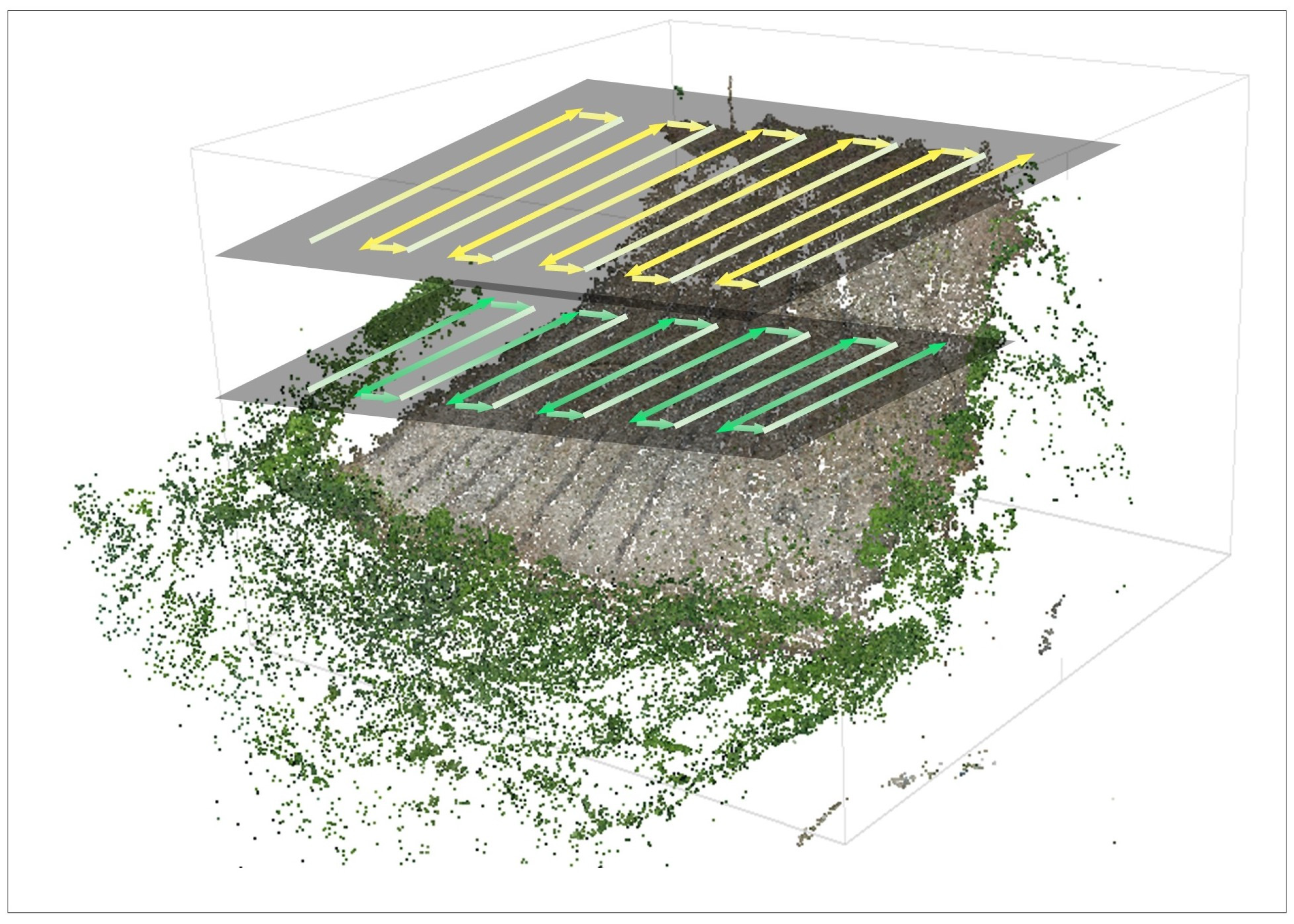
2.2.3. 3D Data Acquisition

All images collected using the automatic flight method were processed photogrammetrically using Agisoft Metashape Professional version 1.5.1 (Agisoft LLC., Petersburg, Russia). In this photogrammetric process, images were used to generate a PCD using the SfM algorithm. Table 1 lists the appropriate settings used in the photo-alignment and dense cloud generation. In the photo-alignment process, the correlation between each photo image was calculated by feature points through SfM, resulting in the generation of tie points and depth maps. In a dense cloud generation, PCDs, which are dense clouds, were generated from tie points.
Geo-referencing was conducted using the GCP points in the Metashape environment. Initially, the GCP points were registered manually in the PCD, and the program automatically selected the corresponding 2D images. The exact centers of the GCP points were manually selected in the 2D images. The center points were manually adjusted and deleted, where relevant, before calculating the GCP center points (distance in cm), which represent the GCP geo-reference errors from June, July, September, and October.

2.3. SSD Detection

Field surveys based on deformation identification are necessary to identify SSDs in the generated 3D data. Each monthly acquired 3D data point (PCD) must be aligned with the GCPs at the lowest spatial RMSE possible for SSD calculation using the DoD method. From the aligned PCDs, DSMs were generated in a geo-referenced coordinate system and further used to calculate the DoD using Agisoft Metashape Professional version 1.5.1. (Agisoft LLC., Petersburg, Russia) and ArcGIS Pro (ESRI Inc., Redlands, CA, USA) at each step.

2.3.1. DSM Generation

Aligned DSMs are required to calculate the height differences between DSMs. Through the photogrammetric process, all 3D data were generated in the PCD format. In many studies, GCPs were used to geo-reference xyz coordinates in PCDs [18,50,51]. In the present study, the coordinates collected from the centers of all 29 GCPs using GNSS were imported into the PCDs in shapefile format. Subsequently, these GCP points were used to apply the coordinate data and validate the spatial error throughout the process.
After alignment by geo-referencing, the PCDs were filtered by extracting ground points and removing large vegetation and noise points on the slope. Filtered PCDs were imported into the Agisoft Metashape Professional version 1.5.1. (Agisoft LLC., Petersburg, Russia) and generated as DEMs and orthomosaics using the WGS 84 (EPSG: 4326) coordinate system (Table 1).

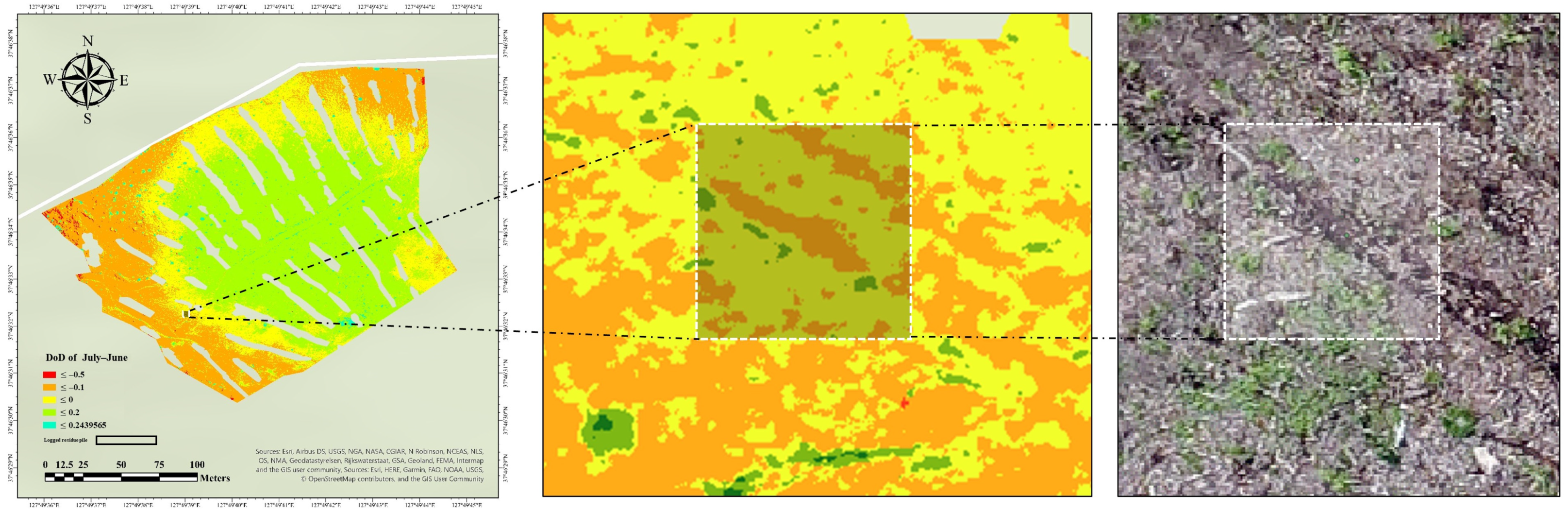
2.3.2. DoD Calculation

The generated DSMs were transferred to ArcGIS Pro for height difference calculations. In ArcGIS Pro, the raster calculator tool is used to calculate the Z values, which represent the height values in the raster files. This method involved subtracting the pixels from the post-DSM from those of the pre-DSM while also considering the resolution during the calculation using Equation (1).
DSM   of   Difference   = post   DSM pre   DSM

2.3.3. Assessments of SSD on Timber Harvesting Site

After calculating the DoD, validation of the height differences at each pixel was required. To verify the precision of the SSD in the DoD, the height values at each installed VP were compared to the VP in the DoD file (Figure 4). The coordinate data acquired from the VPs by GNSS were imported as points in shapefile format on the DoD map. The pixel values calculated using the DoD method were then compared to the GT data recorded in the field survey and calculated as the RMSE for its assessment according to Equation (2).
RMSE   = 1 n i = 1 n e i 2

3. Results

3.1. Data Processing from 2D UAV Imagery

During each UAV flight on 9 June, 10 July, 8 September, and 14 October 2022, 235, 233, 206, and 212 2D images were collected, respectively. These images were aligned and identified as tie points by calculating the correlations for each 2D image, with alignment rates of 97.9% (230/235), 97.9% (228/233), 90.1% (191/212), and 90.3% (186/206), respectively. The tie points were then used to generate dense clouds, which were processed as PCDs in the software (Figure 5). Prior to creating the DEM, filtering and geo-referencing processes were conducted, and the PCDs were extracted for 3D data preprocessing (Table 2). In the geo-referencing process, 29, 28, 27, and 24 GCP coordinates were used for each GCP registration in June, July, September, and October, respectively (Figure 5). However, during the July PCD, spatial distortion occurred when the total RMSE of the GCP registration exceeded 24 cm. Despite the distortion, the total RMSE of the GCP registration between the PCD and GCP coordinates was <13 cm in June, September, and October. After preprocessing the PCD, DEMs were automatically calculated from the PCDs with resolutions < 3 cm, as shown in Table 2. As a result, all DEMs were ready for DoD calculation (Figure 5).

3.2. SSD Detection in Target Area

Acquired DEMs for each period were calculated as a DoD map, i.e., for July–June (Figure 6a), September–July (Figure 6b), October–September (Figure 6c), and October–June (Figure 6d). In the DoD maps, pixels with values < 0 were defined as erosion, and pixels with values > 0 were defined as deposition, according to the DoD equation. Furthermore, erosion areas and average SSD heights were calculated using ArcGIS Pro (ESRI Inc., Redlands, CA, USA) and R version 4.1.3. The calculated erosion area and average SSD heights were approximately 13,293.32 m2 and 13.25 cm in July–June, approximately 9694.4 m2 and 8.38 cm in September–July, and approximately 10,757.63 m2 and 5.13 cm in October–September, respectively. Similarly, deposition area and average SSD heights were calculated as approximately 12,607.99 m2 and 8.2 cm in July–June, 16,206.91 m2 and 23.73 cm in September–July, and 14,579.51 m2 and 5.39 cm in October–September, respectively.
Deposition areas were observed in the center of the timber harvesting area, whereas erosion areas were located at the edges of the DoD from July to June and September to July. The total amounts of erosion and deposition were calculated as the volume (m3) by calculating the area (cm2) and height (cm) of each pixel. From July to June, the total erosion volume was approximately 17.62 m3, and the total deposition volume was 10.33 m3. Moreover, at the end of the monitoring period, the total erosion volume was calculated as 3.38 m3, and the total deposition volume was 28.82 m3, which included the vegetation volume.

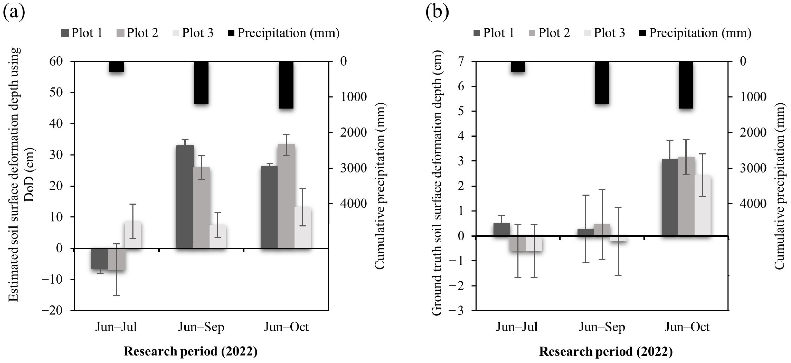
3.3. SSD Validation Using VP Data

Each VP was subtracted from the pixel heights of the field survey points sharing the same coordinates to calculate the total SSD (Figure 7; Table 3). The total RMSE calculated from the 29 VPs was 8.8 cm, representing the average difference between the true data (Table 3). Furthermore, results from the DoD values indicated that the SSDs in Plot 3 were detected with the greatest precision, with the lowest RMSE of 5.64 cm, whereas the SSDs in Plot 2 were detected with the least precision as deposition, with the highest RMSE of 10 cm (Table 3).
The accuracy of the detected SSDs was confirmed through the validation process. Erosion and deposition tendencies were accurately shown for Plots 2 and 3, respectively. However, the RMSEs from both these plots were too high to be considered solely based on the observed tendencies.

3.4. Total SSD from Monitoring

The soil surface of the slope was affected by rainfall over time. On the day of monitoring, a large precipitation event (approximately 1326.7 mm) occurred from a total period of 10 June to 14 October, and the amount of precipitation was recorded in the study area. During monitoring, SSD and surface deformation were calculated as the monthly DoD value for each plot. In the DoD of July–June, erosions were detected in Plots 1 and 2 with average amounts of −6.6 cm and −6.9 cm, respectively, whereas Plot 3 showed deposition of 8.7 cm (Figure 8a). Despite the distortion that occurred from the PCD of July, the average SSD values of all plots were understandable with a tendency comparison of GT (i.e., measured soil deformation). Plot 1 had 0.5 cm, Plot 2 had −0.6 cm, and Plot 3 had −0.6 cm (Figure 8b).
From the DoD of September–June, Plots 1 and 2 showed deposition tendencies with mean DoD values of 32.94 cm and 25.84 cm, respectively, and average GT difference values of 0.29 cm and 0.46 cm, respectively (Figure 8a,b). Plot 3 showed slight deposition compared to the average GT difference values, which were 0.4 cm higher than those during the pre-period (Figure 8b).
During the monitoring period from October to June, all plots demonstrated deposition tendencies. GT values revealed that Plots 1 and 2, which were initially expected to undergo erosion, exhibited deposition by the end of the monitoring period, with 3.1 cm and 3.2 cm of sediment accumulation, respectively (Figure 8b). In contrast, the GT values in Plot 3 did not exhibit a significant increase compared to those in Plots 1 and 2 but rather indicated average deformation of 2.4 cm as a result of deposition (Figure 8b).

4. Discussion

4.1. GCP Registration-Based Geo-Referencing and Distortion Occurred within UAV-Derived 3D Data

Demonstrating the suitability of UAV surveys in forested areas is a challenging task. Moreover, obtaining spatially accurate 3D data without RTK poses a significant challenge [52,53]. A method for determining the number of GCPs to be used in areas < 1 ha and on steep slopes has not yet been defined, even in recent GCP geo-referencing studies [29,54,55,56,57]. Installations of GCPs over stumps enabled an accurate scale of the PCD and geo-referencing [54,56,58,59,60], thereby facilitating the generation of precise 3D data using the GCP coordinates.
A previous representative landslide study [18] was performed in similar UAV survey conditions as in the current study, with flight heights of 100–120 m. The DSM resolution of the study was 10 cm, but the GCP geo-referencing error was given as XY and Z error (2 cm and 6 cm, respectively) [18], making it incomparable to the current study. On the other hand, a previous landslide study [29] revealed that RTK enabled accurate UAV and camera positioning, resulting in GCP RMSE < 4 cm. In contrast to previous studies [18,29,52,53], our photogrammetric procedure revealed that distortions in 2D images may occur randomly during UAV survey image collection and affect forest area data where RTK was not available.
Notably, we found that the distortion increased with the height difference between the UAV and the ground, making GCPs sometimes unidentifiable from UAV flight with GPS mode. For a detailed comparison with other remote-sensing studies, we needed to analyze the accuracy of 3D data alignment to determine the overall error when calculating DoD. Thus, aside from the GCP geo-referencing error results, we analyzed the distance error from the GCP centers in orthomosaics of June, July, September, and October. Our study revealed total average errors of approximately 11.1 cm, 3 cm, and 4.5 cm for the error calculations between July and June orthomosaics, September and June orthomosaics, and October and June orthomosaics, respectively. The geo-referencing results obtained for June, September, and October were highly accurate, even compared to remote-sensing studies [24,29,39,56]. However, due to distortions in the July 3D data, the average error from 3D data alignment in June and July was slightly inaccurate when compared to the errors from June, September, and October. Nonetheless, these errors were still understandable when compared to geo-referencing results from previous studies [24,29,39,56]. Based on the 3D data alignment error analysis, the GPS-based auto-UAV surveys were suitable for steep slopes in areas where the forest canopy has been removed.

4.2. Application of VPFs for Precise Spatial Resolution

UAV surveys were performed with two VPFs at 140 m for the entire non-hazardous research area and 100 m for the lower part of the slope at a high spatial resolution of <3 cm. For comparison purposes, we tested several UAV flights (Table 4), including single flights at an altitude of 140 m and VPFs at altitudes of 140 m and 100 m. We considered flights at speeds of 3 m/s and 5 m/s and side overlaps of 70% and 90% for each flight. The results showed that the resolution increased significantly from approximately 3.5 cm/pix to approximately 2.7 cm/pix. Based on a prior test, we assumed that for reliable UAV surveys without the RTK function, 3D data acquisition on steep slopes requires several VPFs.
We compared the spatial resolutions for steep slopes in this study to those of landslide areas in previous single-flight UAV surveys [23,24,48,61]. In a steep-slope landslide area with elevations of 60–125 m [23], GPS-based UAV surveys were performed with overlaps ranging from 60% to 80% and a flight height of 40 m based on landslides, which resulted in a DSM resolution of 2 cm/pix. In another steep-slope (30–70°) landslide area [48], UAV surveys were performed with overlaps of ~60%, which resulted in DEM resolutions of 2–4 cm/pix. A 5 cm/pix DEM resolution was acquired [24] in UAV surveys with front and side overlaps of 50% and 60%, respectively, and one VPF height of 70 m from the top of the slope. In a study using GNSS-equipped UAV photogrammetry [61], the UAV survey was performed with forward and side overlaps of >90% and >70%, respectively, and a flight height of 60 m, which produced a DEM resolution of 10 cm/pix. A DSM resolution of 2.7 cm/pix has also been acquired from VPFs, which is comparable to high DSM and DEM resolution studies [23,48] that acquired approximately 2 cm/pix. We assumed that the overlaps in our study were comparable to those in a previous GNSS study [61].

4.3. SSD Validation Accuracy and Limitation of Photogrammetric Method on SSD Acquisition

As discussed in Section 3.3, a significant difference was found between the DoD and GT values, which indicated that the average DoD values were approximately 19.7% larger than the average GT values. This phenomenon was due to deposition, including total surface PCD, where small vegetation, such as grass and shrubs, were included but not extracted as ground points in the photogrammetric data, unlike LiDAR data [62,63]. According to previous LiDAR studies [62,63], soil surface DEMs can be generated from original LiDAR-derived PCD by ground point filtering. Especially from [63], the possibility of DEM extraction from DSM was presented by comparing heights of herbaceous points from DSM of SfM and ground data from DEM of LiDAR. However, the method from LiDAR studies [62] was processed with interpolation, such as triangulated irregular network-based refinement that may result in the resolution being sampled in larger centimeters. Thus, we assume that the perfect solution for PCD acquisition on SSDs is not yet developed. Conducting a LiDAR sensor has a better chance of retrieving SSD data accurately compared to the photogrammetric method.
Related studies calculated the RMSE from DEM-derived space-borne and airborne GCP data. However, even with studies related to DEM generation using LiDAR sensors, it is unclear whether these methods are applicable to detecting SSDs. Unlike planform area studies with RMSEs of 5 cm [64] and 7.3 cm [65], the feasibility of application in forest regions, which include steep slopes, remains unknown, as the RMSEs from previous studies were too high for detecting SSD: 15 cm [63], 19 cm [66], and 25 cm [67]. In addition, these previous studies may not be entirely comparable to the present study because the RMSEs were calculated with DEMs or GCPs, not GT and DoD; however, the accuracies from the RMSE of previous studies may be referred to clearly.
As data were processed over time, small vegetation, such as grass, had grown over the research area. Similar to a recent landslide monitoring study [26], we found that dense vegetation covering some parts of landslides inhibited reliable photogrammetric processing and targeted deformation detection. Thus, the only means by which to detect SSDs from the plots was to compare the DoD and GT values in July–June. From the comparison, Plot 2 from the DoD followed the same erosion tendencies as the GT (Figure 8a,b). The calculated distances from GCP points of June and July orthomosaics were determined, and the distortion size on each point was approximately 11 cm, which negatively affected the DoD values. With this limitation, it was clear that it was possible to precisely detect SSDs on Plot 2 (without lower vegetation growth) compared to studies using LiDAR [63]. Despite our study being a case study of UAV photogrammetry in a post-forestry operation area, our findings revealed the potential for SSD detection in estimating the effects of forest soil disturbance by using the DoD method from UAV-derived 3D data. Moreover, we clearly presented the limitation of the photogrammetric method in SSD acquisition for sites where vegetation might grow.

4.4. Monitoring Soil Surface following Timber Harvesting

The aim of this study was to verify whether SSD could be detected after timber harvesting. Object detection necessitates a spatial resolution of less than half the size of the object to be detected [49]. In this study, a DSM was generated with a resolution of <3 cm, enabling the detection of SSDs with a minimum size of 6 × 6 cm. SSDs were identified in the erosion-prone wheel tracks in July–June in Plot 2 (Figure 7). Moreover, the study confirmed that SSDs were detected on logging tracks and their edges in July–June using DoD.
Vegetation growth from October to July was robust, and vegetation covered the VPs, making it impossible to detect SSDs using UAV photogrammetry in all plots. A significant precipitation event occurred between 9 July and 8 September, resulting in positive SSD detections between June and September, whereas GTs indicated erosion. A review [68] revealed that DEM could be obtained from SfM but that it was necessary to have open forest areas. Nonetheless, the present study revealed that even in open-canopy forests, time progression resulted in vegetation growth that covered the soil. Thus, during field surveys on 8 September and 14 October, low vegetation (e.g., grasses) grew in all plots, generating PCDs for low vegetation points rather than the soil surface. Thus, SSDs were not detectable in September or October in areas where vegetation had grown.
Despite the limitations of photogrammetry, monthly surface deformation monitoring revealed that significant precipitation not only affected SSDs but also influenced vegetation growth. The cumulative DoD and GTs for the total monitoring period indicated that soil was marginally deposited as vegetation grew. Moreover, many studies have revealed that soil-slope stability was improved by root systems from the above vegetation cover [69,70,71,72,73]. It is plausible to assume that the slope stability of the timber harvesting area was stabilized as vegetation naturally grew (Figure 8a,b) [69,70,71,72,73].

5. Conclusions

The objective of this study was to detect SSD from UAV 3D data and develop a monitoring approach for steep slopes with canopy openings using UAV photogrammetry techniques. Given the limited comparative studies on SSD detection methodology, this study aimed to identify SSD erosion from photogrammetry data. The VPF method, based on GPS-guided UAV surveys with a spatial resolution of <3 cm was found to be appropriate. However, distortions during the PCD acquisition process were problematic and affected the GCP-based geo-referencing results. Despite these issues, the SSDs were precisely detected from the DoDs as wheel tracks and edges of logging tracks. Moreover, the VPF method enabled safe monitoring of SSDs from DSMs in June, July, September, and October without RTK function. SSDs were evaluated using GT data from the VPs. To conduct SSD monitoring on forest operation sites using UAV photogrammetry, surveys need to be conducted either prior to vegetation growth or during seasons without vegetation. In addition, based on the monitoring that was conducted, it was concluded that the timber harvesting site was stabilized through the assessment of vegetation growth and SSDs shown in the 3D data as an effect of timber harvesting. In future studies, we recommend that improved sensors such as LiDAR be implemented for detecting SSD under vegetation.

Author Contributions

Conceptualization, B.C. and J.K.; Methodology, B.C., J.K. and I.K.; Validation, B.C., J.K. and I.K.; Formal analysis, B.C. and J.K.; Investigation, B.C., I.K., E.H. and J.K.; Resources, B.C. and I.K.; Data curation, B.C., I.K. and E.H.; Writing—original draft preparation, B.C. and J.K.; Writing—review and editing, J.K., I.K., B.C. and E.H.; Visualization, E.H., I.K. and J.K.; Supervision, B.C.; Project administration, B.C.; Funding acquisition, B.C. All authors have read and agreed to the published version of the manuscript.

Funding

This research was carried out with the support of the ‘R&D Program for Forest Science Technology (Project No. 2021367B10-2323-BD01)’ and the ‘R&D Program for Forest Science Technology (Project No. 2019151D10-2323-0301)’ provided by Korea Forest Service (Korea Forestry Promotion Institute).

Data Availability Statement

Not applicable.

Conflicts of Interest

The authors declare no conflict of interest.

References

  1. Worrell, R.; Hampson, A. The influence of some forest operations on the sustainable management of forest soils—A review. Forestry 1997, 70, 61–85. [Google Scholar] [CrossRef]
  2. Grace, J.M. Soil erosion following forest operations in the southern piedmont of central Alabama. J. Soil Water Conserv. 2004, 59, 160–166. [Google Scholar]
  3. Kim, I.; Han, S.K.; Acuna, M.; Woo, H.; Oh, J.H.; Choi, B. Effect of heavy machine traffic on soil CO2 concentration and efflux in a Pinus Koraiensis thinning stand. Forests 2021, 12, 1497. [Google Scholar] [CrossRef]
  4. Aust, W.M.; Blinn, C.R. Forestry best management practices for timber harvesting and site preparation in the eastern united states: An overview of water quality and productivity research during the past 20 years (1982–2002). Water Air Soil Pollut. Focus 2004, 4, 5–36. [Google Scholar] [CrossRef]
  5. Grace, J.M., III. Forest operations and water quality in the south. Trans. ASAE 2005, 48, 871–880. [Google Scholar] [CrossRef]
  6. Choi, B.; Hatten, J.A.; Dewey, J.C.; Otsuki, K.; Cha, D. Effect of timber harvesting on stormflow characteristics in headwater streams of managed, forested watersheds in the upper gulf coastal plain of Mississippi. J. Fac. Agric. Kyushu Univ. 2013, 58, 395–402. [Google Scholar] [CrossRef]
  7. Fielding, J.A.H.; Hawks, B.S.; Aust, W.M.; Bolding, M.C.; Barrett, S.M. Estimated erosion from clearcut timber harvests in the southeastern United States. Forest Sci. 2022, 68, 334–342. [Google Scholar] [CrossRef]
  8. Massey, H.F.; Jackson, M.L. Selective erosion of soil fertility constituents. Soil Sci. Soc. Am. J. 1952, 16, 353–356. [Google Scholar] [CrossRef]
  9. Fox, G.A.; Sheshukov, A.; Cruse, R.; Kolar, R.L.; Guertault, L.; Gesch, K.R.; Dutnell, R.C. Reservoir sedimentation and upstream sediment sources: Perspectives and future research needs on streambank and gully erosion. Environ. Manag. 2016, 57, 945–955. [Google Scholar] [CrossRef]
  10. Bashir, S.; Javed, A.; Bibi, I.; Ahmad, N. Soil and Water Conservation; University of Agriculture: Pakistan, Faisalabad, 2017; pp. 263–286. [Google Scholar]
  11. Elliot, W.J.; Page-Dumroese, D.; Robichaud, P.R. The Effects of Forest Management on Erosion and Soil Productivity. In Soil Quality and Soil Erosion; CRC Press: Boca Raton, FL, USA, 2018; pp. 195–208. [Google Scholar]
  12. Zhou, C.; Wei, X.; Zhou, G.; Yan, J.; Wang, X.; Wang, C.; Liu, H.; Tang, X.; Zhang, Q. Impacts of a large-scale reforestation program on carbon storage dynamics in Guangdong, China. Forest Ecol. Manag. 2008, 255, 847–854. [Google Scholar] [CrossRef]
  13. Hernandez, S.G.; Sheehan, S.W. Comparison of carbon sequestration efficacy between artificial photosynthetic carbon dioxide conversion and timberland reforestation. MRS Energy Sustain. 2020, 7, E32. [Google Scholar] [CrossRef]
  14. Lefebvre, D.; Williams, A.G.; Kirk, G.J.D.; Paul, J.; Burgess, J.; Meersmans, J.; Silman, M.R.; Román-Dañobeytia, F.; Farfan, J.; Smith, P. Assessing the carbon capture potential of a reforestation project. Sci. Rep. 2021, 11, 19907. [Google Scholar] [CrossRef] [PubMed]
  15. Pierzchała, M.; Talbot, B.; Astrup, R. Estimating soil displacement from timber extraction trails in steep terrain: Application of an unmanned aircraft for 3D modelling. Forests 2014, 5, 1212–1223. [Google Scholar] [CrossRef]
  16. Torresan, C.; Berton, A.; Carotenuto, F.; Di Gennaro, S.F.; Gioli, B.; Matese, A.; Miglietta, F.; Vagnoli, C.; Zaldei, A.; Wallace, L. Forestry applications of UAVs in Europe: A review. Int. J. Remote Sens. 2017, 38, 2427–2447. [Google Scholar] [CrossRef]
  17. Cambi, M.; Giannetti, F.; Bottalico, F.; Travaglini, D.; Nordfjell, T.; Chirici, G.; Marchi, E. Estimating machine impact on strip roads via close-range photogrammetry and soil parameters: A case study in central Italy. iForest Biogeosci. For. 2018, 11, 148–154. [Google Scholar] [CrossRef]
  18. Fernández, T.; Pérez, J.L.; Cardenal, J.; Gómez, J.M.; Colomo, C.; Delgado, J. Analysis of landslide evolution affecting olive groves using UAV and photogrammetric techniques. Remote Sens. 2016, 8, 837. [Google Scholar] [CrossRef]
  19. Deligiannakis, G.; Pallikarakis, A.; Papanikolaou, I.; Alexiou, S.; Reicherter, K. Detecting and monitoring early post-fire sliding phenomena using UAV–SfM photogrammetry and t-LiDAR-derived point clouds. Fire 2021, 4, 87. [Google Scholar] [CrossRef]
  20. Sankey, J.B.; Sankey, T.T.; Li, J.; Ravi, S.; Wang, G.; Caster, J.; Kasprak, A. Quantifying plant-soil-nutrient dynamics in rangelands: Fusion of UAV hyperspectral-LiDAR, UAV multispectral-photogrammetry, and ground-based LiDAR-digital photography in a shrub-encroached desert grassland. Remote Sens. Environ. 2021, 253, 112223. [Google Scholar] [CrossRef]
  21. Stumvoll, M.J.; Schmaltz, E.M.; Glade, T. Dynamic characterization of a slow-moving landslide system–assessing the challenges of small process scales utilizing multi-temporal TLS data. Geomorphology 2021, 389, 107803. [Google Scholar] [CrossRef]
  22. Ahmad Fuad, N.; Yusoff, A.R.; Ismail, Z.; Majid, Z. Comparing the performance of point cloud registration methods for landslide monitoring using mobile laser scanning data. Int. Arch. Photogramm. Remote Sens. Spat. Inf. Sci. 2018, 42, 11–21. [Google Scholar] [CrossRef]
  23. Turner, D.; Lucieer, A.; De Jong, S.M. Time series analysis of landslide dynamics using an unmanned aerial vehicle (UAV). Remote Sens. 2015, 7, 1736–1757. [Google Scholar] [CrossRef]
  24. Rossi, G.; Tanteri, L.; Tofani, V.; Vannocci, P.; Moretti, S.; Casagli, N. Multitemporal UAV surveys for landslide mapping and characterization. Landslides 2018, 15, 1045–1052. [Google Scholar] [CrossRef]
  25. Godone, D.; Allasia, P.; Borrelli, L.; Gullà, G. UAV and structure from motion approach to monitor the Maierato Landslide evolution. Remote Sens. 2020, 12, 1039. [Google Scholar] [CrossRef]
  26. Peternel, T.; Janža, M.; Šegina, E.; Bezak, N.; Maček, M. Recognition of landslide triggering mechanisms and dynamics using GNSS, UAV photogrammetry and in situ monitoring data. Remote Sens. 2022, 14, 3277. [Google Scholar] [CrossRef]
  27. Teo, T.A.; Fu, Y.J.; Li, K.W.; Weng, M.C.; Yang, C.M. Comparison between image- and surface-derived displacement fields for landslide monitoring using an unmanned aerial vehicle. Int. J. Appl. Earth Obs. Geoinf. 2023, 116, 103164. [Google Scholar] [CrossRef]
  28. Caturegli, L.; Gaetani, M.; Volterrani, M.; Magni, S.; Minelli, A.; Baldi, A.; Brandani, G.; Mancini, M.; Lenzi, A.; Orlandini, S.; et al. Normalized difference vegetation index versus dark green colour index to estimate nitrogen status on bermudagrass hybrid and tall fescue. Int. J. Remote Sens. 2020, 41, 455–470. [Google Scholar] [CrossRef]
  29. Ellett, N.G.; Pierce, J.L.; Glenn, N.F. Partitioned by process: Measuring post-fire debris-flow and rill erosion with structure from motion photogrammetry. Earth Surf. Process. Landf. 2019, 44, 3128–3146. [Google Scholar] [CrossRef]
  30. Mugnai, F.; Masiero, A.; Angelini, R.; Cortesi, I. Integrating UAS Photogrammetry and Digital Image Correlation for Monitoring of Large Landslides. Preprints 2022, 2022010248. [Google Scholar] [CrossRef]
  31. Nikolakopoulos, K.G.; Kyriou, A.; Koukouvelas, I.K. Developing a guideline of unmanned aerial vehicle’s acquisition geometry for landslide mapping and monitoring. Appl. Sci. 2022, 12, 4598. [Google Scholar] [CrossRef]
  32. Kyriou, A.; Nikolakopoulos, K.G.; Koukouvelas, I.K. Timely and low-cost remote sensing practices for the assessment of landslide activity in the service of hazard management. Remote Sens. 2022, 14, 4745. [Google Scholar] [CrossRef]
  33. Sestras, P.; Bilașco, Ș.; Roșca, S.; Dudic, B.; Hysa, A.; Spalević, V. Geodetic and UAV monitoring in the sustainable management of shallow landslides and erosion of a susceptible urban environment. Remote Sens. 2021, 13, 385. [Google Scholar] [CrossRef]
  34. Kim, I.; Kim, J.; Woo, H.; Choi, B. Feasibility of terrestrial laser scanning system for detecting and monitoring surface displacement of artificial slopes on forest roads. Sens. Mater. 2022, 34, 4787–4799. [Google Scholar] [CrossRef]
  35. Niethammer, U.; Rothmund, S.; James, M.R.; Travelletti, J.; Joswig, M. UAV-based remote sensing of landslides. Int. Arch. Photogramm. Remote Sens. Spat. Inf. Sci. 2010, 38, 496–501. [Google Scholar]
  36. Balaguer-Puig, M.; Marqués-Mateu, Á.; Lerma, J.L.; Ibáñez-Asensio, S. Estimation of small-scale soil erosion in laboratory experiments with structure from motion photogrammetry. Geomorphology 2017, 295, 285–296. [Google Scholar] [CrossRef]
  37. Casagli, N.; Frodella, W.; Morelli, S.; Tofani, V.; Ciampalini, A.; Intrieri, E.; Raspini, F.; Rossi, G.; Tanteri, L.; Lu, P. Spaceborne, UAV and ground-based remote sensing techniques for landslide mapping, monitoring and early warning. Geoenviron. Disasters 2017, 4, 9. [Google Scholar] [CrossRef]
  38. Peppa, M.V.; Mills, J.P.; Moore, P.; Miller, P.E.; Chambers, J.E. Brief communication: Landslide motion from cross correlation of UAV-derived morphological attributes. Nat. Hazards Earth Syst. 2017, 17, 2143–2150. [Google Scholar] [CrossRef]
  39. Carabassa, V.; Montero, P.; Alcañiz, J.M.; Padró, J.C. Soil erosion monitoring in quarry restoration using drones. Minerals 2021, 11, 949. [Google Scholar] [CrossRef]
  40. Conoscenti, C.; Martinello, C.; Alfonso-Torreño, A.; Gómez-Gutiérrez, Á. Predicting sediment deposition rate in check-dams using machine learning techniques and high-resolution DEMs. Environ. Earth Sci. 2021, 80, 380. [Google Scholar] [CrossRef]
  41. Assouline, S.; Ben-Hur, M. Effects of rainfall intensity and slope gradient on the dynamics of interrill erosion during soil surface sealing. Catena 2006, 66, 211–220. [Google Scholar] [CrossRef]
  42. Neugirg, F.; Kaiser, A.; Schmidt, J.; Becht, M.; Haas, F. Quantification, analysis and modelling of soil erosion on steep slopes using LiDAR and UAV photographs. Proc. Int. Assoc. Hydrol. Sci. 2015, 367, 51–58. [Google Scholar] [CrossRef]
  43. Yang, C.; Su, Z.A.; Fan, J.R.; Fang, H.D.; Shi, L.T.; Zhang, J.H.; He, Z.; Zhou, T.; Wang, X.Y. Simulation of the landform change process on a purple soil slope due to tillage erosion and water erosion using UAV technology. J. Mt. Sci. 2020, 17, 1333–1344. [Google Scholar] [CrossRef]
  44. Lucieer, A.; Jong, S.M.D.; Turner, D. Mapping landslide displacements using structure from motion (SfM) and Image correlation of multi-temporal UAV photography. Prog. Phys. Geogr. 2014, 38, 97–116. [Google Scholar] [CrossRef]
  45. Xu, Q.; Li, W.L.; Ju, Y.Z.; Dong, X.J.; Peng, D.L. Multitemporal UAV-based photogrammetry for landslide detection and monitoring in a large area: A case study in the Heifangtai Terrace in the Loess Plateau of China. J. Mt. Sci. 2020, 17, 1826–1839. [Google Scholar] [CrossRef]
  46. Kyriou, A.; Nikolakopoulos, K.; Koukouvelas, I. How image acquisition geometry of UAV campaigns affects the derived products and their accuracy in areas with complex geomorphology. ISPRS Int. J. Geo Inf. 2021, 10, 408. [Google Scholar] [CrossRef]
  47. Fernández, T.; Pérez, J.L.; Cardenal, F.J.; López, A.; Gómez, J.M.; Colomo, C.; Delgado, J.; Sánchez, M. Use of a light UAV and photogrammetric techniques to study the evolution of a landslide in Jaén (Southern Spain). Int. Arch. Photogramm. Remote Sens. Spat. Inf. Sci. 2015, 40, 241–248. [Google Scholar] [CrossRef]
  48. Peternel, T.; Kumelj, Š.; Oštir, K.; Komac, M. Monitoring the Potoška Planina Landslide (NW Slovenia) using UAV photogrammetry and tachymetric measurements. Landslides 2017, 14, 395–406. [Google Scholar] [CrossRef]
  49. Jensen, J.R. Introductory Digital Image Processing: A Remote Sensing Perspective, 3rd ed.; Prentice Hall Inc.: Hoboken, NJ, USA, 2005. [Google Scholar]
  50. Erenoğlu, R.C.; Erenoğlu, O. A case study on the comparison of terrestrial methods and unmanned aerial vehicle technique in landslide surveys: Sarıcaeli Landslide, Çanakkale, NW Turkey. Int. J. Environ. Geoinf. 2018, 5, 325–336. [Google Scholar] [CrossRef]
  51. Dinkov, D.; Kitev, A. Advantages, Disadvantages and Applicability of GNSS Post-Processing Kinematic (PPK) Method for Direct Georeferencing of UAV Images. In Proceedings of the 8th International Conference on Cartography and GIS, Nessebar, Bulgaria, 20–25 June 2020; pp. 15–20. [Google Scholar]
  52. Furukawa, F.; Laneng, L.A.; Ando, H.; Yoshimura, N.; Kaneko, M.; Morimoto, J. Comparison of RGB and multispectral unmanned aerial vehicle for monitoring vegetation coverage changes on a landslide area. Drones 2021, 5, 97. [Google Scholar] [CrossRef]
  53. Ilinca, V.; Șandric, I.; Chițu, Z.; Irimia, R.; Gheuca, I. UAV Applications to assess short-term dynamics of slow-moving landslides under dense forest cover. Landslides 2022, 19, 1717–1734. [Google Scholar] [CrossRef]
  54. Sanz-Ablanedo, E.; Chandler, J.H.; Rodríguez-Pérez, J.R.; Ordóñez, C. Accuracy of unmanned aerial vehicle (UAV) and SfM photogrammetry survey as a function of the number and location of ground control points used. Remote Sens. 2018, 10, 1606. [Google Scholar] [CrossRef]
  55. Cho, J.; Lee, J.; Lee, B. Application of UAV photogrammetry to slope-displacement measurement. KSCE J. Civ. Eng. 2022, 26, 1904–1913. [Google Scholar] [CrossRef]
  56. Huang, H.; Long, J.; Lin, H.; Zhang, L.; Yi, W.; Lei, B. Unmanned aerial vehicle based remote sensing method for monitoring a steep mountainous slope in the Three Gorges Reservoir, China. Earth Sci. Inform. 2017, 10, 287–301. [Google Scholar] [CrossRef]
  57. Liu, X.; Lian, X.; Yang, W.; Wang, F.; Han, Y.; Zhang, Y. Accuracy assessment of a UAV direct georeferencing method and impact of the configuration of ground control points. Drones 2022, 6, 30. [Google Scholar] [CrossRef]
  58. Yurtseven, H. Comparison of GNSS-, TLS-and different altitude UAV-generated datasets on the basis of spatial differences. ISPRS Int. J. Geo Inf. 2019, 8, 175. [Google Scholar] [CrossRef]
  59. Villanueva, J.K.S.; Blanco, A.C. Optimization of ground control point (GCP) configuration for unmanned aerial vehicle (UAV) survey using structure from motion (SFM). Int. Arch. Photogramm. Remote Sens. Spat. Inf. Sci. 2019, 42, 167–174. [Google Scholar] [CrossRef]
  60. Meinen, B.U.; Robinson, D.T. Streambank topography: An accuracy assessment of UAV-based and traditional 3D reconstructions. Int. J. Remote Sens. 2020, 41, 1–18. [Google Scholar] [CrossRef]
  61. Eker, R.; Aydın, A.; Hübl, J. Unmanned aerial vehicle (UAV)-based monitoring of a landslide: Gallenzerkogel Landslide (Ybbs-Lower Austria) case study. Environ. Monit. Assess. 2018, 190, 28. [Google Scholar] [CrossRef]
  62. Chen, Z.; Gao, B.; Devereux, B. State-of-the-Art: DTM generation using airborne LIDAR Data. Sensors 2017, 17, 150. [Google Scholar] [CrossRef]
  63. Moudrý, V.; Gdulová, K.; Fogl, M.; Klápště, P.; Urban, R.; Komárek, J.; Moudrá, L.; Štroner, M.; Barták, V.; Solský, M. Comparison of leaf-off and leaf-on combined UAV imagery and airborne LiDAR for assessment of a post-mining site terrain and vegetation structure: Prospects for monitoring hazards and restoration success. Appl. Geogr. 2019, 104, 32–41. [Google Scholar] [CrossRef]
  64. García-López, S.; Vélez-Nicolás, M.; Zarandona-Palacio, P.; Curcio, A.C.; Ruiz-Ortiz, V.; Barbero, L. UAV-borne LiDAR revolutionizing groundwater level mapping. Sci. Total Environ. 2023, 859, 160272. [Google Scholar] [CrossRef]
  65. Li, H.; Ye, W.; Liu, J.; Tan, W.; Pirasteh, S.; Fatholahi, S.N.; Li, J. High-resolution terrain modeling using airborne lidar data with transfer learning. Remote Sens. 2021, 13, 3448. [Google Scholar] [CrossRef]
  66. Estornell, J.; Ruiz, L.A.; Velázquez-Martí, B.; Hermosilla, T. Analysis of the factors affecting LiDAR DTM accuracy in a steep shrub area. Int. J. Digit. Earth 2011, 4, 521–538. [Google Scholar] [CrossRef]
  67. Cosenza, D.N.; Gomes Pereira, L.; Guerra-Hernández, J.; Pascual, A.; Soares, P.; Tomé, M. Impact of calibrating filtering algorithms on the quality of LiDAR-derived DTM and on forest attribute estimation through area-based approach. Remote Sens. 2020, 12, 918. [Google Scholar] [CrossRef]
  68. Iglhaut, J.; Cabo, C.; Puliti, S.; Piermattei, L.; O’Connor, J.; Rosette, J. Structure from motion photogrammetry in forestry: A review. Curr. For. Rep. 2019, 5, 155–168. [Google Scholar] [CrossRef]
  69. Wu, T.H. Effect of vegetation on slope stability. Transp. Res. Rec. 1984, 965, 37–46. [Google Scholar]
  70. Greenwood, J.R.; Norris, J.E.; Wint, J. Assessing the contribution of vegetation to slope stability. Proc. Inst. Civ. Eng. Geotech. Eng. 2004, 157, 199–207. [Google Scholar] [CrossRef]
  71. Cammeraat, E.; van Beek, R.; Kooijman, A. Vegetation succession and its consequences for slope stability in SE Spain. Plant Soil 2005, 278, 135–147. [Google Scholar] [CrossRef]
  72. Schwarz, M.; Preti, F.; Giadrossich, F.; Lehmann, P.; Or, D. Quantifying the role of vegetation in slope stability: A case study in Tuscany (Italy). Ecol. Eng. 2010, 36, 285–291. [Google Scholar] [CrossRef]
  73. Kokutse, N.K.; Temgoua, A.G.T.; Kavazović, Z. Slope stability and vegetation: Conceptual and numerical investigation of mechanical effects. Ecol. Eng. 2016, 86, 146–153. [Google Scholar] [CrossRef]
Figure 1. Location and panoramic view of timber harvesting area in experiment forest of Kangwon National University.
Forests 14 00980 g001
Figure 2. GCP-GNSS implemented on a tree stump installed GCPs and validation point (VP)-GNSS for field survey; (a) GCP installed on a tree stump, (b) VP data collection, and (c) VP installed on soil surface displacement (SSD) of a wheel track.
Forests 14 00980 g002
Figure 3. Vertically parallel flight (VPF) method for acquisition of monthly UAV-derived point cloud data (PCD); flight paths were separated at 100 m and 140 m. For a 100 m flight (green line), 2D images were collected with 110 shots, and for a 140 m flight (yellow line), 2D images were collected with 90 shots, respectively, per flight.
Forests 14 00980 g003
Figure 4. The locations of plots and installed validation points (VPs) are used to confirm soil surface deformation (SSD) amounts in the DoD. (a) DoD of July–June, (b) wheel track (Plot 2), (c) erosion expected area (Plot 1), and (d) deposition expected area (Plot 3). The points and the numbers presented in each plot are locations of installed VPs.
Forests 14 00980 g004
Figure 5. Monthly acquired point cloud data (PCD) and digital surface model (DSM) from GCP registration. (a) PCD and DSM for 10 June, (b) PCD and DSM for 9 July, (c) PCD and DSM for 8 September, and (d) PCD and DSM for 14 October. The points presented on these 3D data are GCP points.
Forests 14 00980 g005
Figure 6. Calculated DoD by pre-month and post-month. (a) DoD of June–July, (b) DoD of July–September, (c) DoD of October–September, and (d) DoD of October–June.
Forests 14 00980 g006
Figure 7. Detection of wheel track erosion from DoD of July–June and orthomosaic of 9 July.
Forests 14 00980 g007
Figure 8. Monthly cumulative surface deformation occurred at the erosion expected area (Plot 1), wheel track (Plot 2), and deposition expected area (Plot 3). (a) cumulative DoD differences related to cumulative precipitation, and (b) cumulative GT differences related to cumulative precipitation.
Forests 14 00980 g008
Table 1. Parameters used in each process to generate 3D data.
ProcessParameterSetting
Align Photos2D images input140 m + 100 m
AccuracyHighest
Reference preselectionOn
Key point limit40,000
Tie point limit4000
Build Dense CloudQualityUltra-high
Depth filteringAggressive
Build DSMProjectionWGS 84 (EPSG: 4326)
Source dataDense cloud
Point classesAll
Build OrthomosaicProjectionWGS 84 (EPSG: 4326)
SurfaceDEM
Table 2. Statistical results of 3D data acquisition.
2022
JuneJulySeptemberOctober
Tie points224,667204,202161,039183,479
Raw PCD238,094,337126,297,339117,432,867140,461,664
Segmented
PCD for DSM
97,027,87088,692,24185,499,11983,302,596
DSM resolution (cm/pix)2.682.652.732.67
Geo-referencing error (cm)12.9424.2412.1312.34
Total DoD area (ha)2.53
Table 3. Estimated soil surface deformation depth on validation point (VP) using DoD and measured soil surface deformation depth (ground truth; GT) on validation point (VP).
Plot 1
(Erosion Expected Area)
Plot 2
(Wheel Track)
Plot 3
(Deposition Expected Area)
VP
No.
GT
(cm)
DoD Value (cm)VP
No.
GT
(cm)
DoD Value (cm)VP
No.
GT
(cm)
DoD Value (cm)
11.30.31111.16.721−3.5−10.5
20.21.112−0.17.422−1.5−7.6
30.28.313−2.63.523−5−6.7
4−0.62.6140.66.624−2.3−8.5
50.410.315−2.93.2
6−3.610.716−1.211.0
7−0.64.417−1.2−6.5
8−0.812.318−0.211.2
9410.719−1.911.7
10−1.57.120−4.513.5
Table 4. Flights performed for comparison of vertically parallel flights (VPFs) and single flights at 140 m and 100 m.
Auto Flight OptionsDSM Resolution
(cm/pix)
Flight SpeedSide
Overlap
Forward OverlapFlight
Altitude
(m/s)(%)(%)(m)
39080100 + 1402.78
37080100 + 1402.55
59080100 + 1402.67
57080100 + 1402.57
390801403.04
370801403.54
590801403.54
570801403.6
Disclaimer/Publisher’s Note: The statements, opinions and data contained in all publications are solely those of the individual author(s) and contributor(s) and not of MDPI and/or the editor(s). MDPI and/or the editor(s) disclaim responsibility for any injury to people or property resulting from any ideas, methods, instructions or products referred to in the content.

