
Modeling Wildfire Initial Attack Success Rate Based on Machine Learning in Liangshan, China


Abstract
1. Introduction
2. Materials and Methods
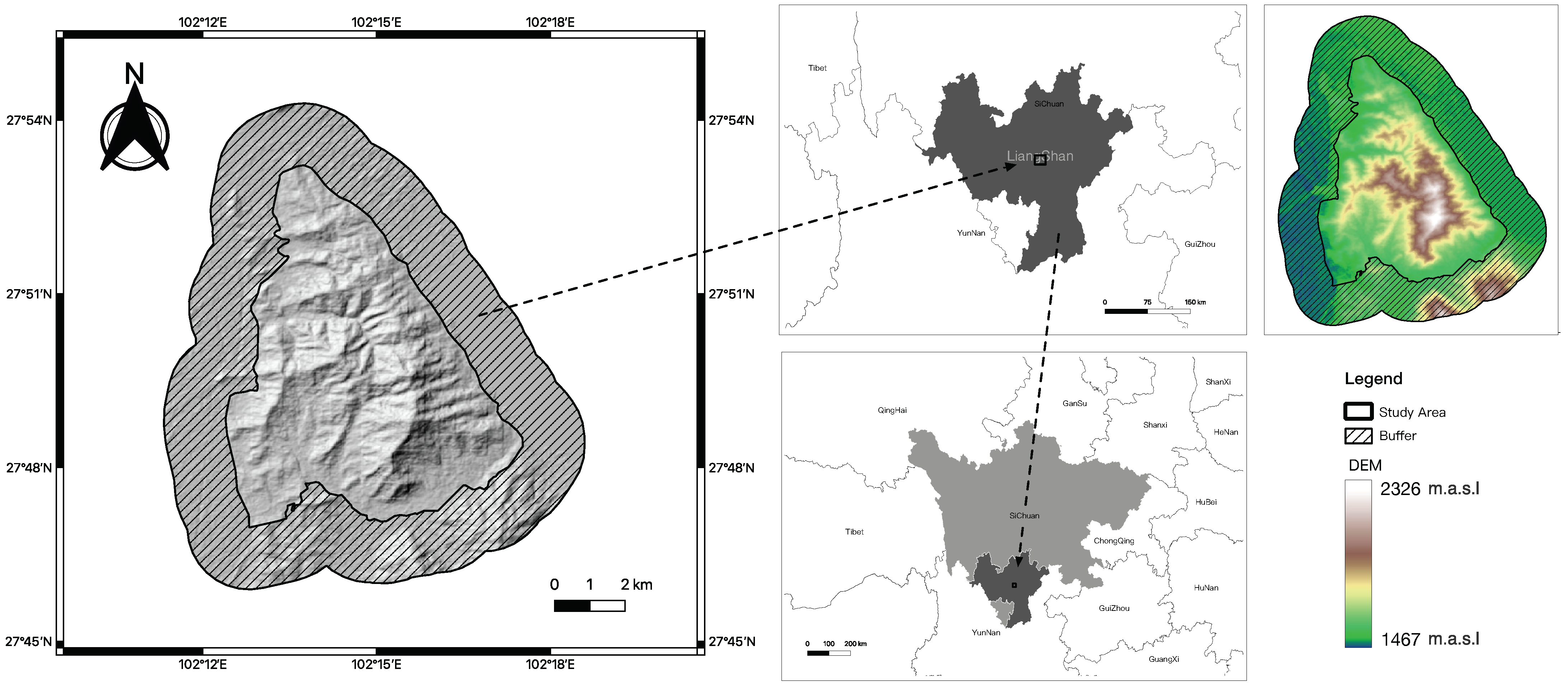
2.1. Study Area
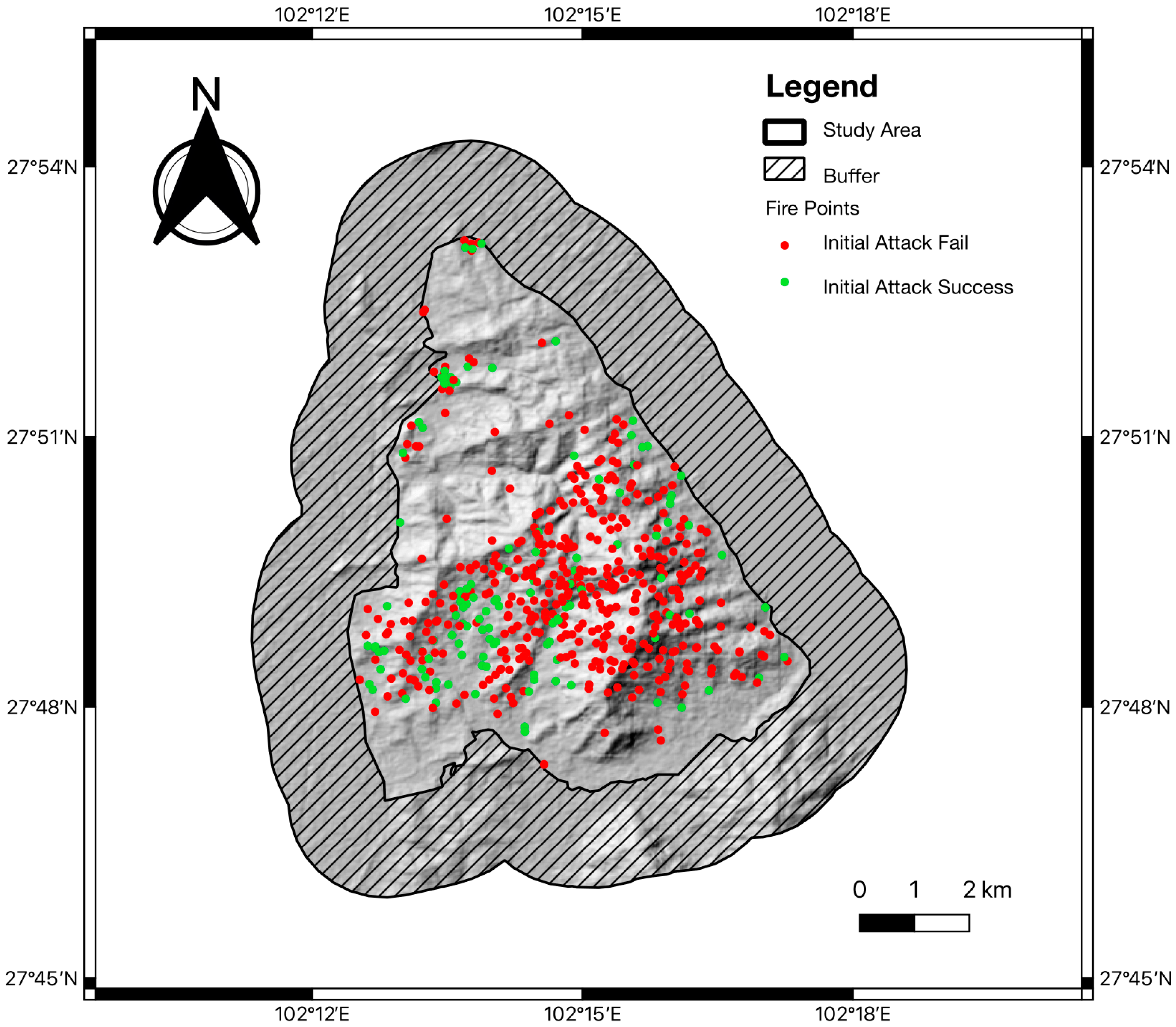
2.2. Data Source
2.3. Feature Selection
2.3.1. Initial Attack Delay
- (1)
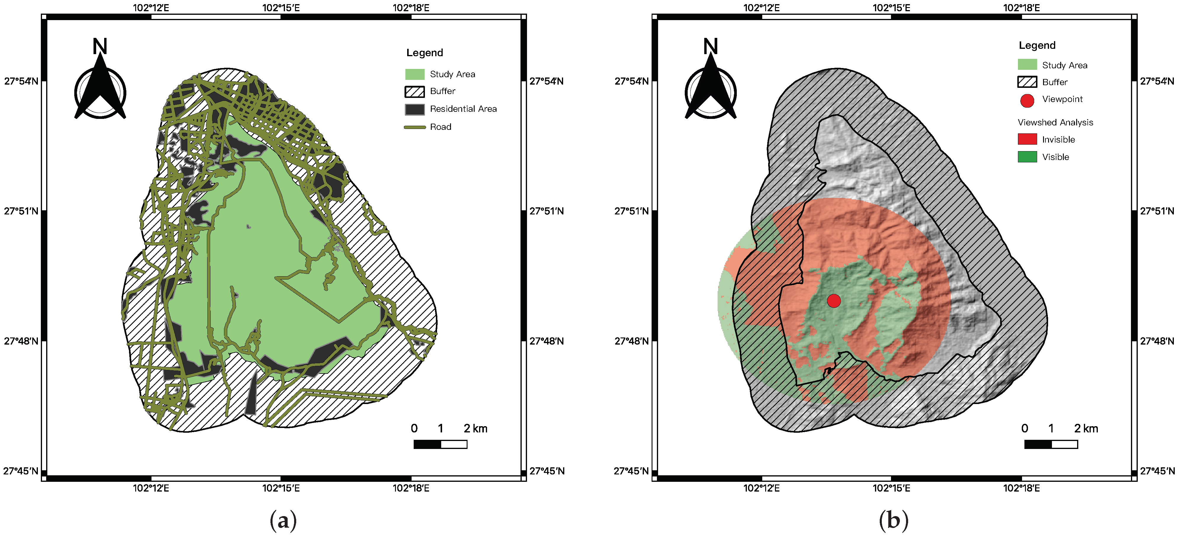
- The size of the sight field of the fire point
- (2)
- Time period of fire
- (3)
- The brightness of the fire point
- (4)
- Thermal radiation from the fire point
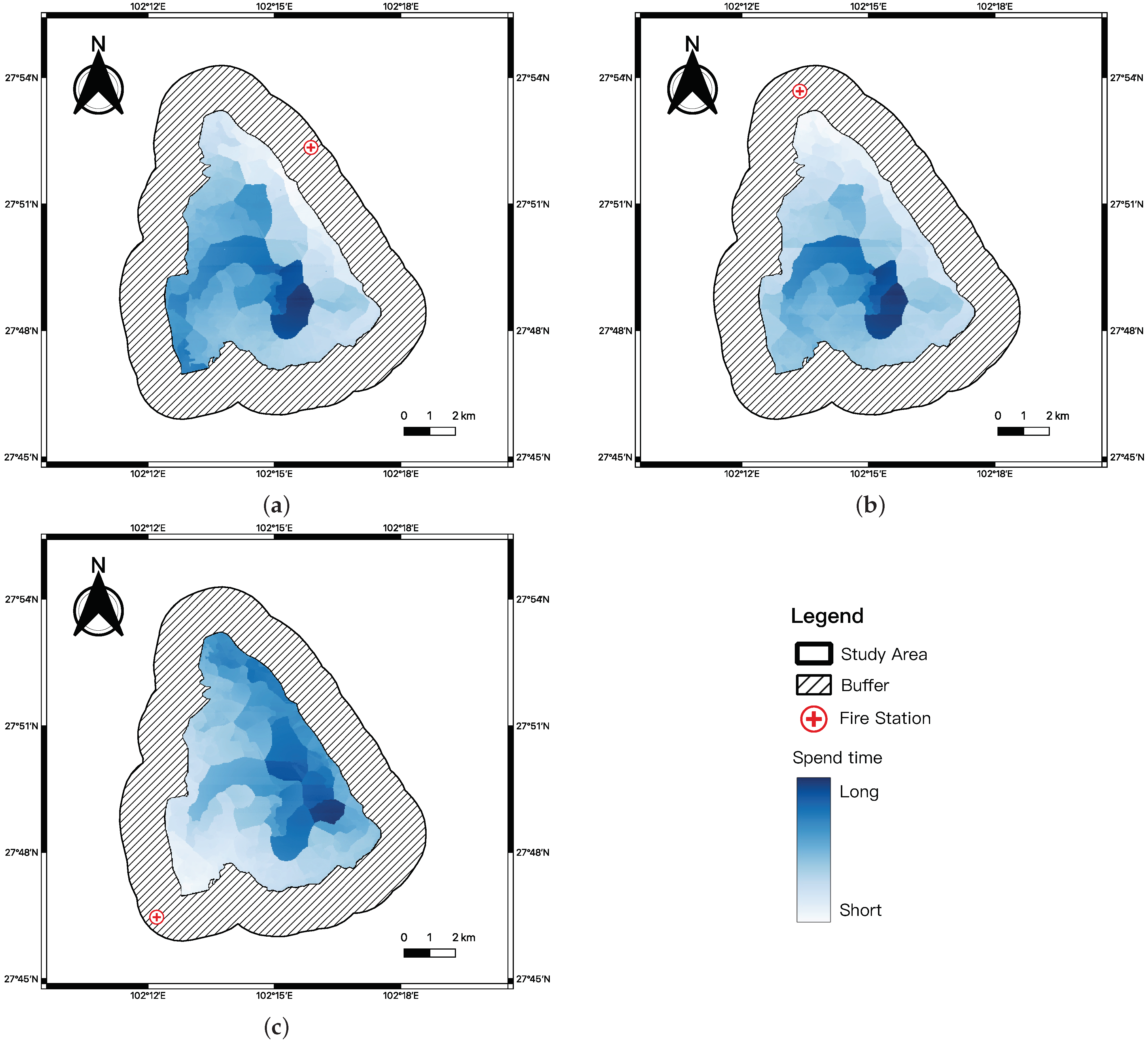
2.3.2. Arrival Time
2.3.3. Spread Potential
- (1)
- Weather factor
- (2)
- Vegetation density
- (3)
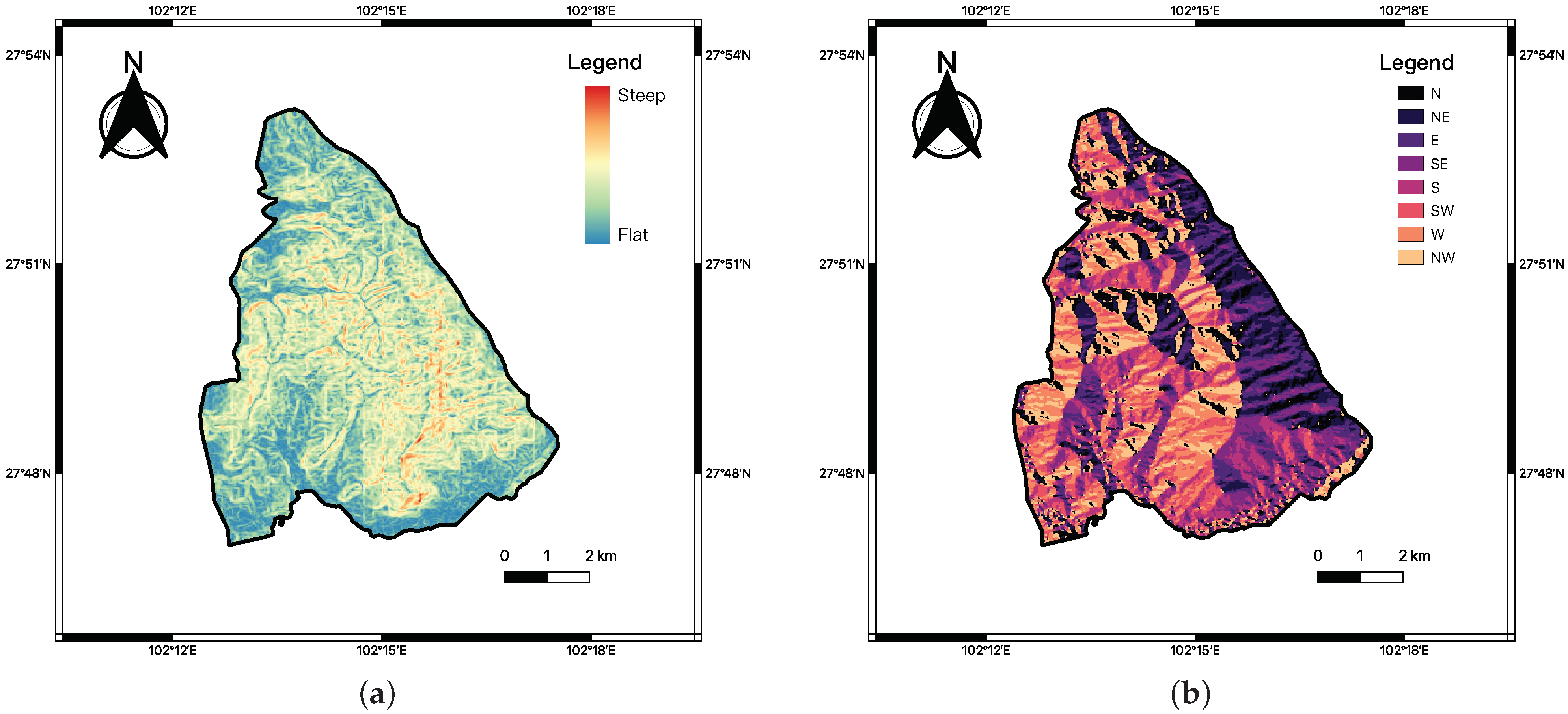
- Topography
2.3.4. Wildfire Fighting Capability
2.4. Feature Pretreatment
2.4.1. SMOTE Oversampling
2.4.2. Correlation Analysis
2.5. Machine Learning Model
2.5.1. Logical Regression
2.5.2. XGBoost
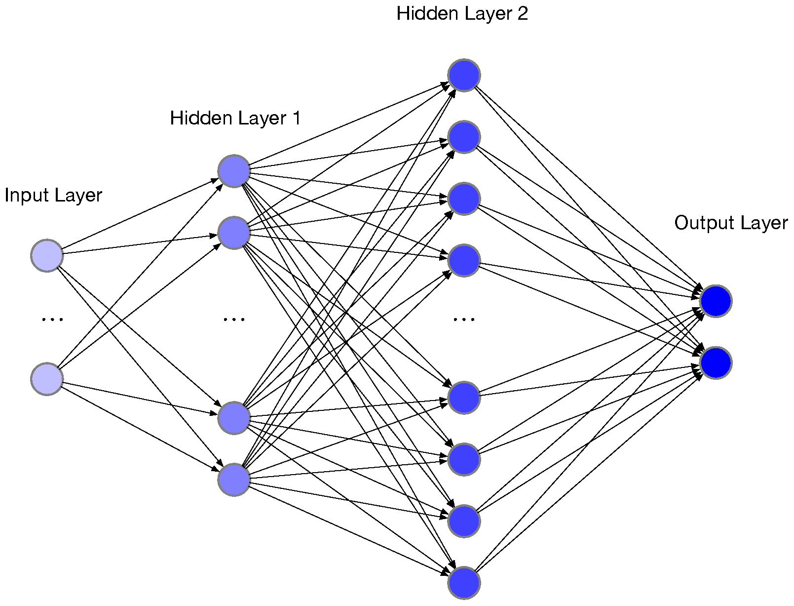
2.5.3. Artificial Neural Networks
3. Results and Discussion
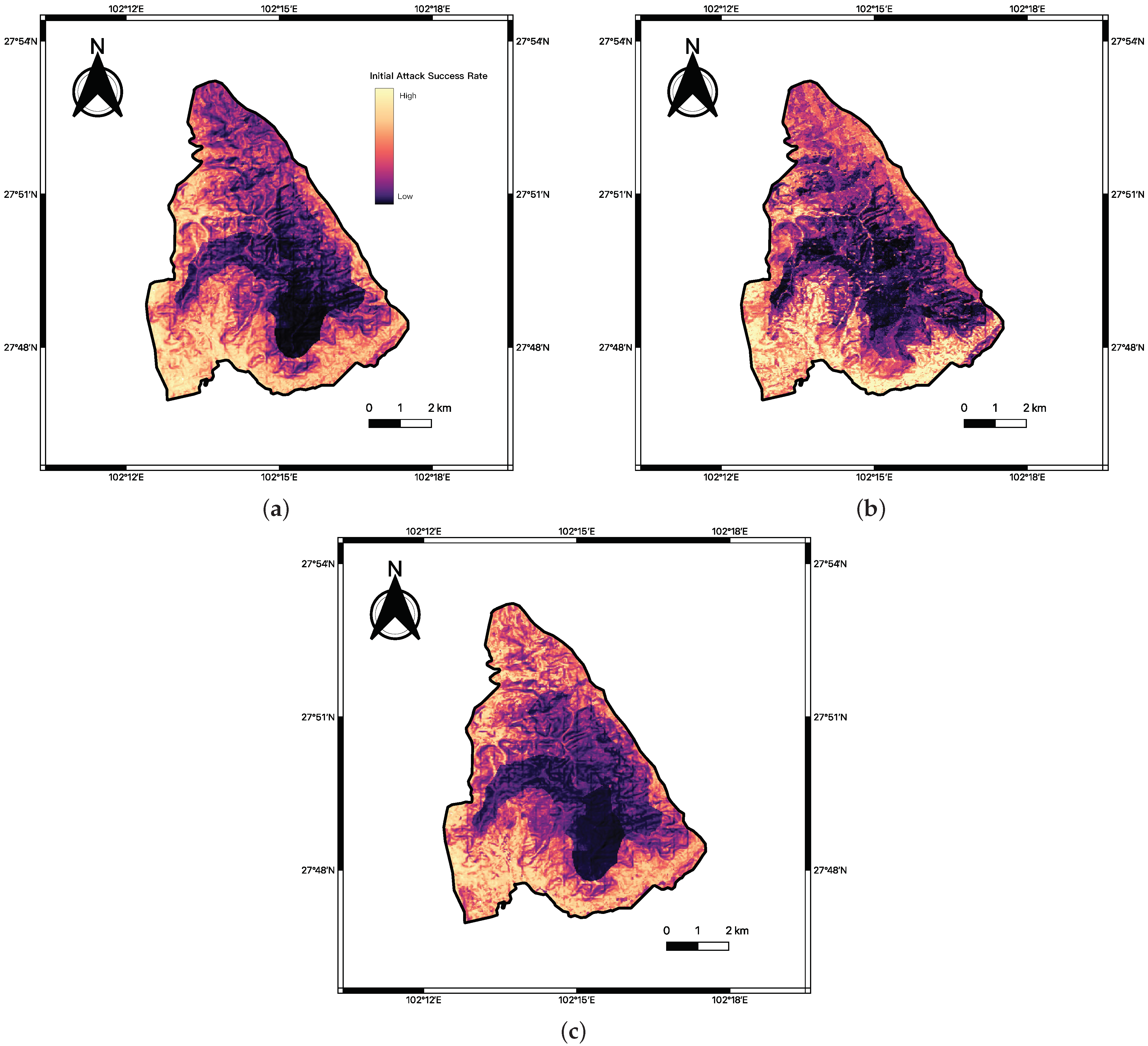
3.1. Normal Weather
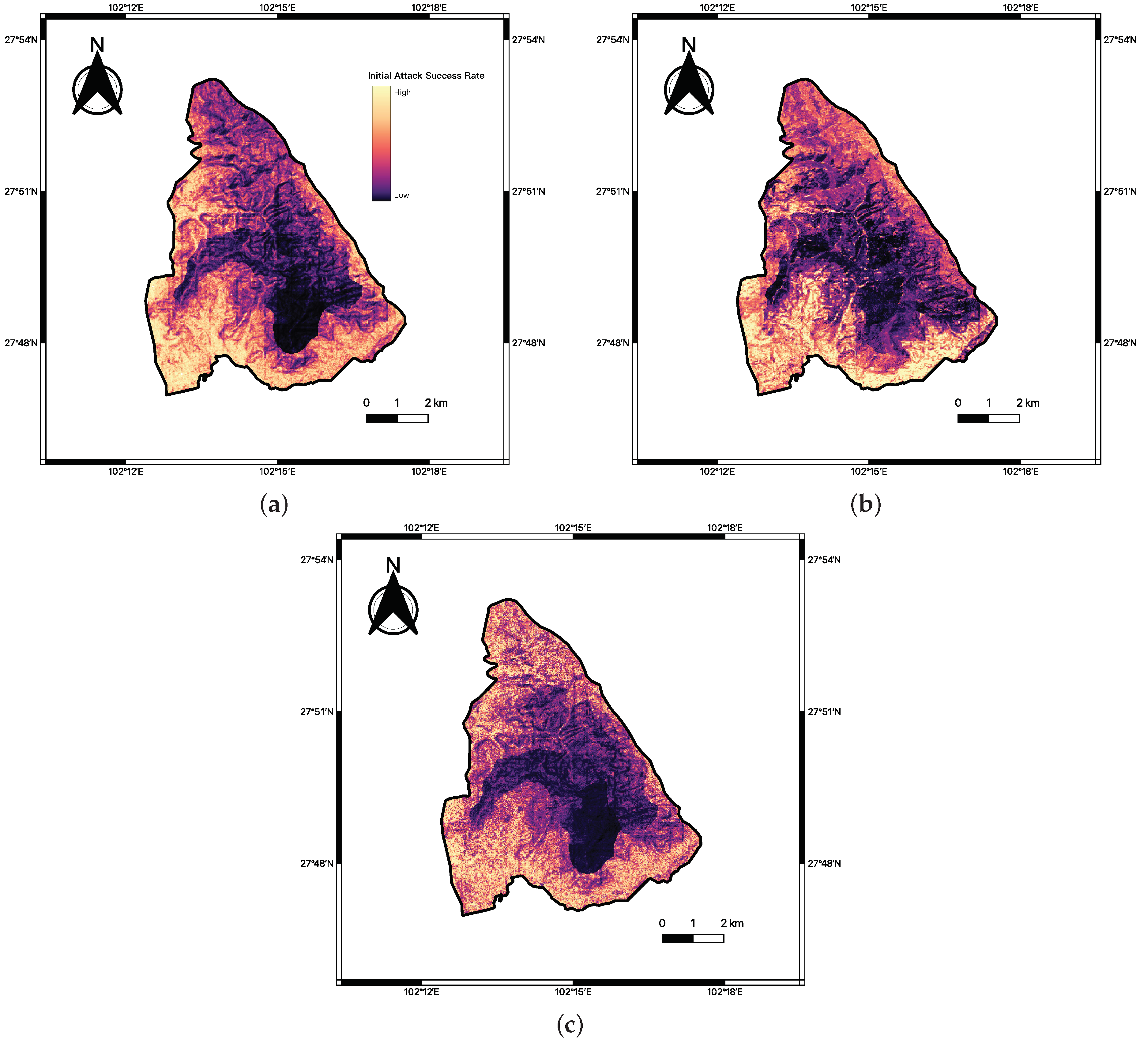
3.2. Extreme Weather
3.3. Comparison under Different Scenes
3.4. Model Evaluation
4. Conclusions
Author Contributions
Funding
Data Availability Statement
Conflicts of Interest
References
- Zhan, Z. Li Keqiang Made Important Instructions on Forest and Grassland Fire Prevention and Control Work. Mod. Occup. Saf. 2020. Available online: http://www.xinhuanet.com/politics/2020-09/18/c_1126513000.htm (accessed on 13 February 2023).
- Gao, C.; Lin, H.L.; Hu, H.Q.; Song, H. A review of models of forest fire occurrence prediction in China. Ying Yong Sheng Tai Xue Bao J. Appl. Ecol. 2020, 31, 3227–3240. [Google Scholar]
- Cao, Y.; Wang, M.; Liu, K. Wildfire susceptibility assessment in Southern China: A comparison of multiple methods. Int. J. Disaster Risk Sci. 2017, 8, 164–181. [Google Scholar] [CrossRef]
- Zhong, M.; Fan, W.; Liu, T.; Li, P. Statistical analysis on current status of China forest fire safety. Fire Saf. J. 2003, 38, 257–269. [Google Scholar] [CrossRef]
- Zhang, F.; Dong, Y.; Xu, S.; Yang, X.; Lin, H. An approach for improving firefighting ability of forest road network. Scand. J. For. Res. 2020, 35, 547–561. [Google Scholar] [CrossRef]
- Paudel, A.; Martell, D.L.; Woolford, D.G. Factors that affect the timing of the dispatch of initial attack resources to forest fires in northeastern Ontario, Canada. Int. J. Wildland Fire 2018, 28, 15–24. [Google Scholar] [CrossRef]
- Lee, Y.; Fried, J.S.; Albers, H.J.; Haight, R.G. Deploying initial attack resources for wildfire suppression: Spatial coordination, budget constraints, and capacity constraints. Can. J. For. Res. 2013, 43, 56–65. [Google Scholar] [CrossRef]
- Reimer, J.; Thompson, D.K.; Povak, N. Measuring initial attack suppression effectiveness through burn probability. Fire 2019, 2, 60. [Google Scholar] [CrossRef]
- Arienti, M.C.; Cumming, S.G.; Boutin, S. Empirical models of forest fire initial attack success probabilities: The effects of fuels, anthropogenic linear features, fire weather, and management. Can. J. For. Res. 2006, 36, 3155–3166. [Google Scholar] [CrossRef]
- Beverly, J.L. Time since prior wildfire affects subsequent fire containment in black spruce. Int. J. Wildland Fire 2017, 26, 919–929. [Google Scholar] [CrossRef]
- Cardil, A.; Lorente, M.; Boucher, D.; Boucher, J.; Gauthier, S. Factors influencing fire suppression success in the province of Quebec (Canada). Can. J. For. Res. 2019, 49, 531–542. [Google Scholar] [CrossRef]
- Tremblay, P.O.; Duchesne, T.; Cumming, S.G. Survival analysis and classification methods for forest fire size. PLoS ONE 2018, 13, e0189860. [Google Scholar] [CrossRef]
- Podur, J.J.; Martell, D.L. A simulation model of the growth and suppression of large forest fires in Ontario. Int. J. Wildland Fire 2007, 16, 285–294. [Google Scholar] [CrossRef]
- Gonzalez-Olabarria, J.R.; Reynolds, K.M.; Larrañaga, A.; Garcia-Gonzalo, J.; Busquets, E.; Pique, M. Strategic and tactical planning to improve suppression efforts against large forest fires in the Catalonia region of Spain. For. Ecol. Manag. 2019, 432, 612–622. [Google Scholar] [CrossRef]
- Rashidi, E.; Medal, H.; Hoskins, A. An attacker-defender model for analyzing the vulnerability of initial attack in wildfire suppression. Nav. Res. Logist. (NRL) 2018, 65, 120–134. [Google Scholar] [CrossRef]
- Collins, K.M.; Price, O.F.; Penman, T.D. Suppression resource decisions are the dominant influence on containment of Australian forest and grass fires. J. Environ. Manag. 2018, 228, 373–382. [Google Scholar] [CrossRef]
- Minas, J.; Hearne, J.; Martell, D. An integrated optimization model for fuel management and fire suppression preparedness planning. Ann. Oper. Res. 2015, 232, 201–215. [Google Scholar] [CrossRef]
- Mendes, A.B.; e Alvelos, F.P. Iterated local search for the placement of wildland fire suppression resources. Eur. J. Oper. Res. 2022. [Google Scholar] [CrossRef]
- Ntaimo, L.; Arrubla, J.A.G.; Stripling, C.; Young, J.; Spencer, T. A stochastic programming standard response model for wildfire initial attack planning. Can. J. For. Res. 2012, 42, 987–1001. [Google Scholar] [CrossRef]
- Ntaimo, L.; Gallego-Arrubla, J.A.; Gan, J.; Stripling, C.; Young, J.; Spencer, T. A simulation and stochastic integer programming approach to wildfire initial attack planning. For. Sci. 2013, 59, 105–117. [Google Scholar] [CrossRef]
- Wei, Y.; Bevers, M.; Belval, E.J. Designing seasonal initial attack resource deployment and dispatch rules using a two-stage stochastic programming procedure. For. Sci. 2015, 61, 1021–1032. [Google Scholar] [CrossRef]
- Rodrigues, M.; Alcasena, F.; Vega-García, C. Modeling initial attack success of wildfire suppression in Catalonia, Spain. Sci. Total Environ. 2019, 666, 915–927. [Google Scholar] [CrossRef] [PubMed]
- Marshall, E.; Dorph, A.; Holyland, B.; Filkov, A.; Penman, T.D. Suppression resources and their influence on containment of forest fires in Victoria. Int. J. Wildland Fire 2022, 31, 1144–1154. [Google Scholar] [CrossRef]
- Jia, L. Research on Forest Fire Prevention and Control Countermeasures in Liangshan Prefecture. For. Fire Prev. 2019, 3, 9–14. [Google Scholar]
- Chander, G.; Markham, B.L.; Helder, D.L. Summary of current radiometric calibration coefficients for Landsat MSS, TM, ETM+, and EO-1 ALI sensors. Remote Sens. Environ. 2009, 113, 893–903. [Google Scholar] [CrossRef]
- Mutanga, O.; Kumar, L. Google Earth Engine Applications; MDPI: Basel, Switzerland, 2019. [Google Scholar]
- Gorelick, N.; Hancher, M.; Dixon, M.; Ilyushchenko, S.; Thau, D.; Moore, R. Google Earth Engine: Planetary-scale geospatial analysis for everyone. Remote Sens. Environ. 2017, 202, 18–27. [Google Scholar] [CrossRef]
- Giglio, L.; Descloitres, J.; Justice, C.O.; Kaufman, Y.J. An enhanced contextual fire detection algorithm for MODIS. Remote Sens. Environ. 2003, 87, 273–282. [Google Scholar] [CrossRef]
- Xofis, P.; Konstantinidis, P.; Papadopoulos, I.; Tsiourlis, G. Integrating remote sensing methods and fire simulation models to estimate fire hazard in a south-east mediterranean protected area. Fire 2020, 3, 31. [Google Scholar] [CrossRef]
- Keane, R.E.; Burgan, R.; van Wagtendonk, J. Mapping wildland fuels for fire management across multiple scales: Integrating remote sensing, GIS, and biophysical modeling. Int. J. Wildland Fire 2001, 10, 301–319. [Google Scholar] [CrossRef]
- Plucinski, M.P. Factors affecting containment area and time of Australian forest fires featuring aerial suppression. For. Sci. 2012, 58, 390–398. [Google Scholar] [CrossRef]
- Plucinski, M.P. Modelling the probability of Australian grassfires escaping initial attack to aid deployment decisions. Int. J. Wildland Fire 2012, 22, 459–468. [Google Scholar] [CrossRef]
- Wooster, M.; Roberts, G.; Freeborn, P.; Xu, W.; Govaerts, Y.; Beeby, R.; He, J.; Lattanzio, A.; Fisher, D.; Mullen, R. LSA SAF Meteosat FRP products–Part 1: Algorithms, product contents, and analysis. Atmos. Chem. Phys. 2015, 15, 13217–13239. [Google Scholar] [CrossRef]
- Cuckovic, Z. Advanced viewshed analysis: A Quantum GIS plug-in for the analysis of visual landscapes. J. Open Source Softw. 2016, 1, 32. [Google Scholar] [CrossRef]
- Pettorelli, N.; Vik, J.O.; Mysterud, A.; Gaillard, J.M.; Tucker, C.J.; Stenseth, N.C. Using the satellite-derived NDVI to assess ecological responses to environmental change. Trends Ecol. Evol. 2005, 20, 503–510. [Google Scholar] [CrossRef] [PubMed]
- Myneni, R.B.; Hall, F.G.; Sellers, P.J.; Marshak, A.L. The interpretation of spectral vegetation indexes. IEEE Trans. Geosci. Remote Sens. 1995, 33, 481–486. [Google Scholar] [CrossRef]
- Lydersen, J.M.; North, M.P.; Collins, B.M. Severity of an uncharacteristically large wildfire, the Rim Fire, in forests with relatively restored frequent fire regimes. For. Ecol. Manag. 2014, 328, 326–334. [Google Scholar] [CrossRef]
- Prichard, S.J.; Kennedy, M.C. Fuel treatments and landform modify landscape patterns of burn severity in an extreme fire event. Ecol. Appl. 2014, 24, 571–590. [Google Scholar] [CrossRef]
- Chawla, N.V.; Bowyer, K.W.; Hall, L.O.; Kegelmeyer, W.P. SMOTE: Synthetic minority over-sampling technique. J. Artif. Intell. Res. 2002, 16, 321–357. [Google Scholar] [CrossRef]
- Maalouf, M. Logistic regression in data analysis: An overview. Int. J. Data Anal. Tech. Strateg. 2011, 3, 281–299. [Google Scholar] [CrossRef]
- Pedregosa, F.; Varoquaux, G.; Gramfort, A.; Michel, V.; Thirion, B.; Grisel, O.; Blondel, M.; Prettenhofer, P.; Weiss, R.; Dubourg, V.; et al. Scikit-learn: Machine Learning in Python. J. Mach. Learn. Res. 2011, 12, 2825–2830. [Google Scholar]
- Hosmer, D.W., Jr.; Lemeshow, S.; Sturdivant, R.X. Applied Logistic Regression; John Wiley & Sons: Hoboken, NJ, USA, 2013; Volume 398. [Google Scholar]


| Data | Description | Source |
|---|---|---|
| Landsat 7 | NDVI (2008–2013) | https://developers.google.com/earth-engine/data (access date: 2 April 2022) |
| Landsat 8 | NDVI (2014–2021) | https://developers.google.com/earth-engine/datasets (access date: 2 April 2022) |
| ASTGTMv003 | Slope, Aspect | https://lpdaac.usgs.gov/products/astgtmv003/ (access date: 2 April 2022) |
| MODIS | Fire points Distribution, Brightness, Thermal Radiation | https://earthdata.nasa.gov/earth-observation-data/near-real-time/firms/about-firms (access date: 2 April 2022) |
| S-NPP | Fire points Distribution, Brightness, Thermal Radiation | https://earthdata.nasa.gov/earth-observation-data/near-real-time/firms/about-firms (access date: 2 April 2022) |
| NOAA-20 | Fire points Distribution, Brightness, Thermal Radiation | https://earthdata.nasa.gov/earth-observation-data/near-real-time/firms/about-firms (access date: 2 April 2022) |
| OSM | Road network | https://www.openstreetmap.org/ (access date: 2 April 2022) |
| CDRs | Temperature, Wind speed, Wind direction | https://www.ncei.noaa.gov/products/climate-data-records (access date: 2 April 2022) |
| Grading | Speed Interval (km/h) | Description |
|---|---|---|
| Walking Road | 0–20 | Vehicles are difficult to pass and can pass a limited number of pedestrians. |
| Third Class Highway | 30–40 | The terrain is more tortuous and can only pass small vehicles |
| Second Class Highway | 60–80 | Set with single lane, flat terrain, able to pass through medium-sized vehicles |
| First Class Highway | 80–100 | There are multiple lanes, which can accommodate multiple large vehicles at the same time |
| Machine Learning Model | Initial Scene | Number of Escape Fire Points | Escape Rate (%) | Escape Rate Increase (%) |
|---|---|---|---|---|
| logistic regression | Normal weather | 14,927 | 22.22% | N/A |
| logistic regression | Extreme weather | 15,144 | 22.54% | 0.32% |
| XGBoost | Normal weather | 15,112 | 22.49% | N/A |
| XGBoost | Extreme weather | 15,432 | 22.97% | 0.48% |
| Artificial neural network | Normal weather | 14,926 | 22.22% | N/A |
| Artificial neural network | Extreme weather | 16,015 | 23.84% | 1.62% |
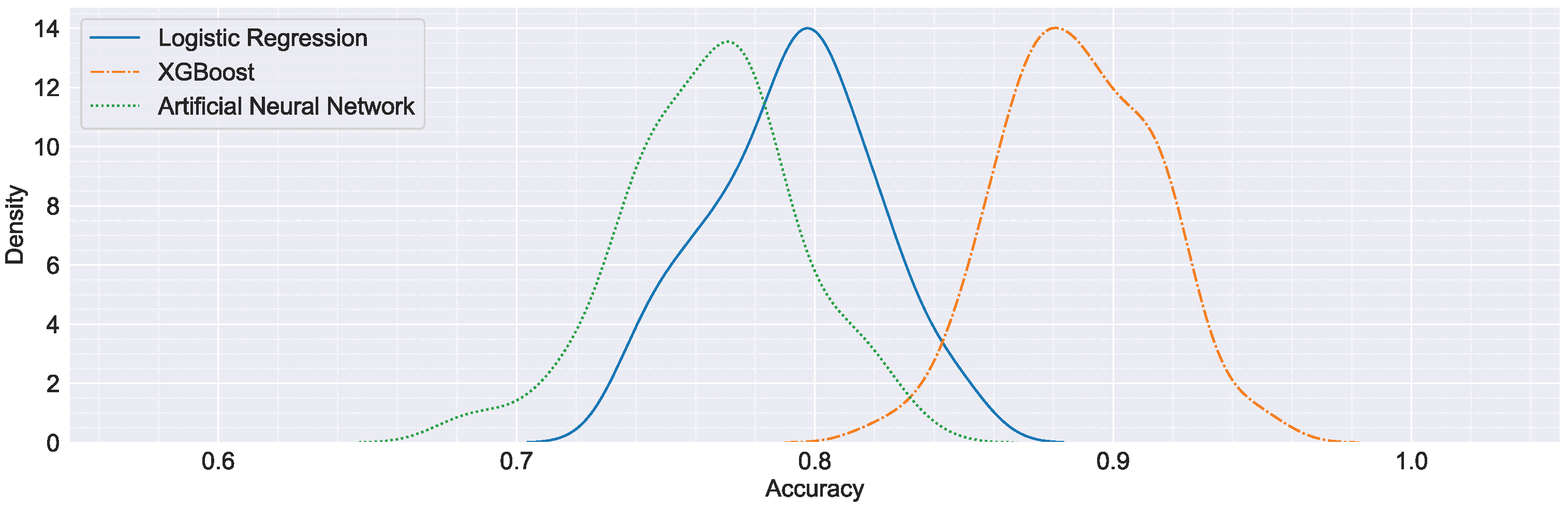
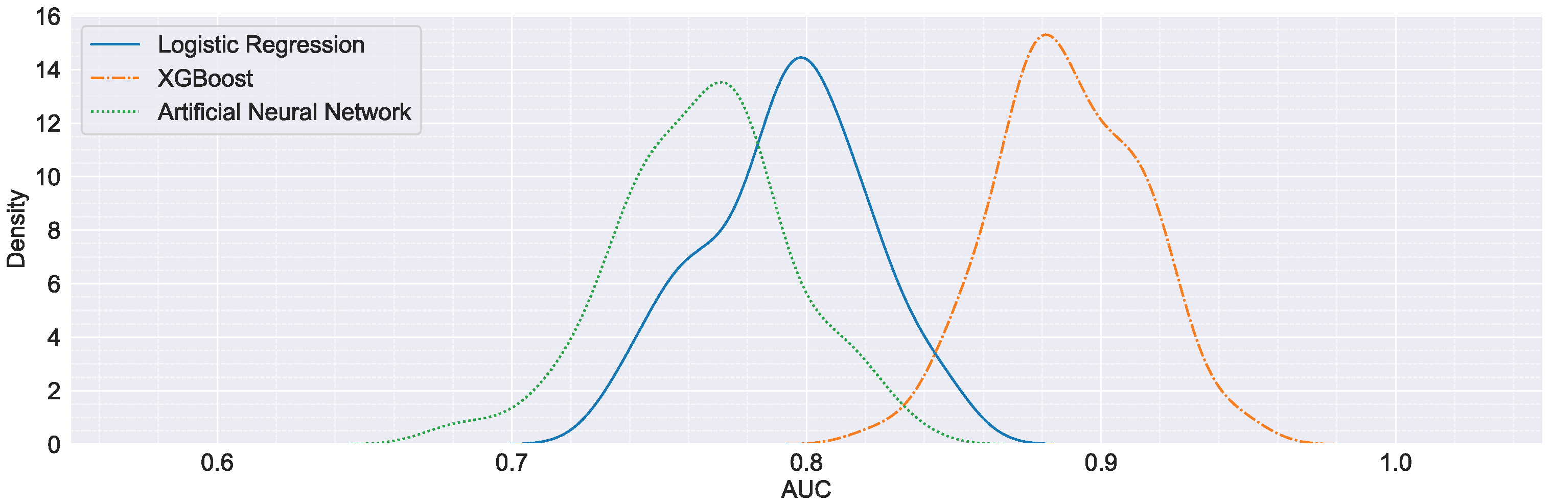
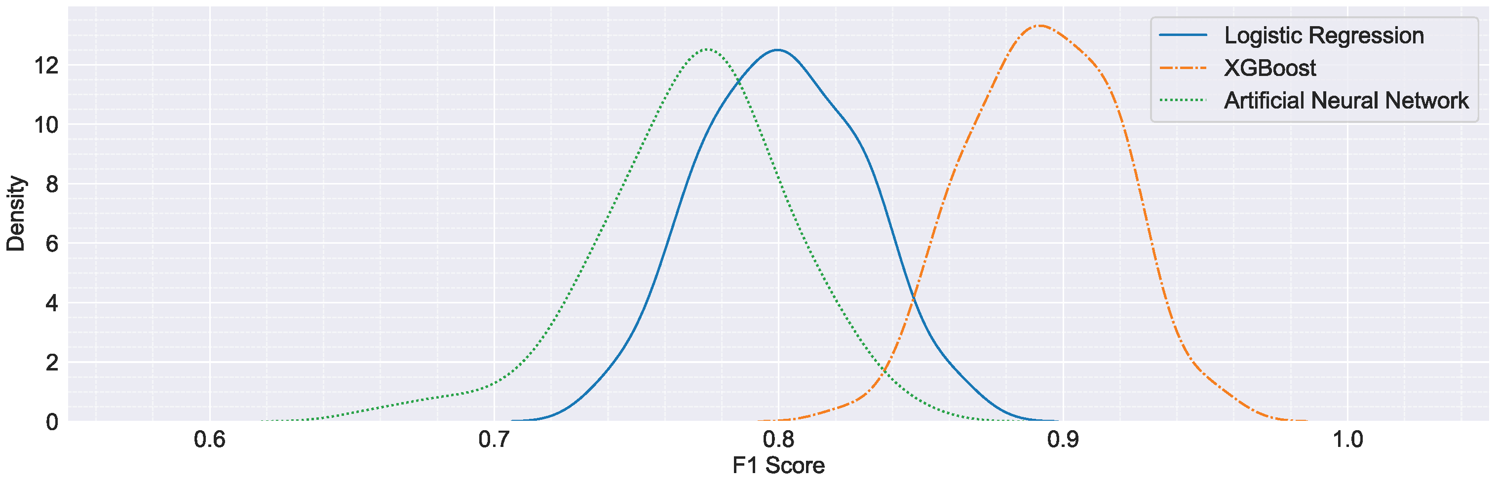
| Model | LR | XGBoost | ANN | ||||||
|---|---|---|---|---|---|---|---|---|---|
| Accuracy | AUC | F1 Score | Accuracy | AUC | F1 Score | Accuracy | AUC | F1 Score | |
| mean | 0.793 | 0.793 | 0.801 | 0.888 | 0.889 | 0.893 | 0.764 | 0.764 | 0.77 |
| std | 0.028 | 0.027 | 0.028 | 0.025 | 0.025 | 0.026 | 0.03 | 0.03 | 0.034 |
| min | 0.737 | 0.733 | 0.739 | 0.82 | 0.823 | 0.824 | 0.683 | 0.681 | 0.658 |
| 25% | 0.772 | 0.777 | 0.779 | 0.868 | 0.873 | 0.876 | 0.743 | 0.745 | 0.752 |
| 50% | 0.796 | 0.795 | 0.802 | 0.886 | 0.887 | 0.894 | 0.766 | 0.766 | 0.771 |
| 75% | 0.81 | 0.811 | 0.822 | 0.91 | 0.906 | 0.913 | 0.784 | 0.782 | 0.79 |
| max | 0.85 | 0.851 | 0.865 | 0.952 | 0.95 | 0.956 | 0.832 | 0.832 | 0.846 |
Disclaimer/Publisher’s Note: The statements, opinions and data contained in all publications are solely those of the individual author(s) and contributor(s) and not of MDPI and/or the editor(s). MDPI and/or the editor(s) disclaim responsibility for any injury to people or property resulting from any ideas, methods, instructions or products referred to in the content. |
© 2023 by the authors. Licensee MDPI, Basel, Switzerland. This article is an open access article distributed under the terms and conditions of the Creative Commons Attribution (CC BY) license (https://creativecommons.org/licenses/by/4.0/).
Share and Cite
Xu, Y.; Zhou, K.; Zhang, F. Modeling Wildfire Initial Attack Success Rate Based on Machine Learning in Liangshan, China. Forests 2023, 14, 740. https://doi.org/10.3390/f14040740
Xu Y, Zhou K, Zhang F. Modeling Wildfire Initial Attack Success Rate Based on Machine Learning in Liangshan, China. Forests. 2023; 14(4):740. https://doi.org/10.3390/f14040740
Chicago/Turabian StyleXu, Yiqing, Kaiwen Zhou, and Fuquan Zhang. 2023. "Modeling Wildfire Initial Attack Success Rate Based on Machine Learning in Liangshan, China" Forests 14, no. 4: 740. https://doi.org/10.3390/f14040740
APA StyleXu, Y., Zhou, K., & Zhang, F. (2023). Modeling Wildfire Initial Attack Success Rate Based on Machine Learning in Liangshan, China. Forests, 14(4), 740. https://doi.org/10.3390/f14040740