Article

Estimation of Forest Stock Volume Combining Airborne LiDAR Sampling Approaches with Multi-Sensor Imagery

1
Key Laboratory of Sustainable Forest Ecosystem Management—Ministry of Education, School of Forestry, Northeast Forestry University, Harbin 150040, China
2
Engineering Consulting & Design Institute, Northeast Forestry University, Harbin 150040, China
*
Author to whom correspondence should be addressed.
Forests 2023, 14(12), 2453; https://doi.org/10.3390/f14122453
Submission received: 22 November 2023 / Revised: 8 December 2023 / Accepted: 14 December 2023 / Published: 15 December 2023
(This article belongs to the Section Forest Inventory, Modeling and Remote Sensing)

Abstract

:
Timely and reliable estimation of forest stock volume is essential for sustainable forest management and conservation. Light detection and ranging (LiDAR) data can provide an effective depiction of the three-dimensional structure information of forests, but its large-scale application is hampered by spatial continuity. This study aims to construct a LiDAR sampling framework, combined with multi-sensor imagery, to estimate the regional forest stock volume of natural secondary forests in Northeast China. Two sampling approaches were compared, including systematic sampling and classification-based sampling. First, the forest stock volume was mapped using a combination of field measurement data and full-coverage LiDAR data. Then, the forest stock volume obtained in the first step of estimation was used as a reference value, and optical images and topographic features were combined for secondary modeling to compare the effectiveness and accuracy of different sampling methods, including 12 systematic sampling and classification-based sampling methods. Our results show that the root mean square error (RMSE) of the 12 systematic sampling approaches ranged from 55.81 to 57.42 m3/ha, and the BIAS ranged from 21.55 to 24.89 m3/ha. The classification-based LiDAR sampling approach outperformed systematic sampling, with an RMSE of 55.56 (<55.81 m3/ha) and a BIAS of 20.68 (<21.55 m3/ha). This study compares different LiDAR sampling approaches and explores an effective LiDAR sample collection scheme for estimating forest stock, while balancing cost and accuracy. The classification-based LiDAR sampling approach described in this study is easy to apply and portable and can provide a reference for future LiDAR sample collection.

1. Introduction

Forest ecosystems are an important component of terrestrial ecosystems and play a vital role in maintaining the global carbon balance [1]. To quantitatively evaluate forest quality and its continuous spatial distribution, a timely and reliable forest inventory is needed, and forest stock volume is one of the important measurement parameters [2].
Traditionally, forest surveys rely on the collection of field data from sample plots, where the stand-level volume is obtained by aggregating the volumes of individual trees, requiring measurements for each tree [3,4,5]. Such surveys are time-consuming, labor-intensive, and space-limited. Integration of various remote sensing data with field measurements has been an effective method for the spatially continuous estimation of forest stock volume [6,7]. Optical imagery, which can receive forest canopy reflections through sensors, was first applied to estimate forest stock volume [8,9]. However, optical imagery can only provide partial horizontal structural information about the forest and is affected by cloud cover, leading to saturation issues in forest stock volume estimation [10]. Active microwave sensors can perform ground observations throughout the day and under all weather conditions, and they have a certain ability to penetrate the surface [11]. However, there is still a saturation problem in estimating forest stock volume above 200 m3/ha in high-density forests [12]. In recent years, LiDAR has been able to accurately and comprehensively reconstruct the three-dimensional structure information of forests using laser scanners in a short period. This capability reduces saturation problems and improves the accuracy of forest stock volume estimation [13,14]. However, the collection of LiDAR data is often limited by accessibility, cost, flight policies, etc., making it difficult to obtain spatially continuous data [15]. Therefore, it is still considered auxiliary data in large-scale forest surveys and mapping.
Compared to multispectral imagery, hyperspectral imagery covers more discrete spectral bands, allowing it to capture more subtle spectral features. With the continuous advancement of technology and improvement in data processing capabilities, hyperspectral imagery has a wide range of applications in forest resource management, monitoring forest health, and tree species identification [16,17,18,19]. Wan et al. used Landsat 8, Simulated Hyperion, and GF-5 datasets to classify four mangrove tree species. It was shown that the classification accuracy of the GF-5 satellite reached 87.12%, which may be attributed to the improvement in spectral resolution (spectral resolution of 5 nm) for enhancing the classification accuracy [20]. Kaja Kandare et al. used airborne LiDAR and hyperspectral imagery to estimate overall and species-specific volumes in Italian alpine forests and concluded that both LiDAR and hyperspectral metrics were important for estimating forest stock volumes, with an RMSE of 30.95% for estimating plot volumes [21]. Almeida et al. fused airborne hyperspectral and LiDAR data for aboveground biomass estimation in tropical forests. The results showed that the most important hyperspectral features were related to the near-infrared and shortwave infrared bands, especially the canopy water and lignin–cellulose absorption bands [22].
Different remote sensing data have distinct advantages and disadvantages in forest stock volume estimation. Satellite-borne spectral images offer comprehensive spectral characteristics at a relatively low cost but lack the ability to capture vertical characteristics [23]. On the other hand, LiDAR can provide accurate vertical geometric features of the forest [24]. Despite their respective limitations [25,26], fusing LiDAR and hyperspectral data offers a dual advantage: (1) leveraging the strengths of both datasets; and (2) utilizing an appropriate sampling approach without the need for full-coverage LiDAR. This fusion method enhances the utilization of diverse data sources, addressing limitations and thereby improving estimation accuracy and efficiency [27]. The fusion approach involves using LiDAR data as an intermediate sample to connect measured plots with full-coverage imagery in two steps. Initially, the measured volume is combined with LiDAR variables, and subsequently, the satellite prediction factors model the estimated volume of LiDAR data, generating forest stock volume estimation results and maps [28,29]. Additionally, the digital elevation model (DEM) of the Advanced Land Observing Satellite (ALOS) provides accurate topographic information, which is helpful for estimating forest stock volume [30].
The LiDAR sampling approach significantly influences estimation outcomes, with different methods yielding varied results. It is recommended to use the LiDAR sampling approach that best aligns with the overall distribution of the study area to achieve the best accuracy in forest parameter estimation. Common LiDAR sampling approaches include random sampling, systematic sampling, and stratified sampling by land cover [31]. Systematic sampling refers to extracting samples (points, lines, grids) at predetermined intervals. Tsui et al. utilized systematic grid sampling at different intervals (500 m, 1000 m, 2000 m) for LiDAR sampling to predict biomass over a larger area [32]. Hudak et al. used different intervals (250 m, 500 m, 1000 m, 2000 m) with different systematic sampling (points, lines) for LiDAR to estimate and map regional forest canopy height in combination with Landsat ETM+ data [33]. Systematic sampling is relatively simple and easy to apply, but it tends to ignore the heterogeneity within the study area, which may lead to under-coverage in specific regions. In contrast, classification-based sampling allows a targeted sample selection based on different classes or characteristics, enhancing sample representation [27]. Chen and Hay used optical images with LiDAR strips to simulate full-coverage forest canopy height, revealing that optimal LiDAR strips had similar canopy height variations as the entire LiDAR dataset [34]. Previous studies have considered systematic sampling and classification-based sampling, but few have compared these two sampling methods.
This study aims to explore the application of LiDAR sampling combined with multi-sensor imagery in estimating forest stock volume. Although the value of LiDAR sampling has been widely recognized and various sampling approaches have been proposed, there is still a lack of widely accepted and cost-effective LiDAR sampling protocols for estimating forest stock volume. In addition, although forest type has always been considered an important factor in volume estimation, there have been few studies on LiDAR sampling based on forest type classification and combined with multi-sensor imagery for volume estimation. This study combines field data, various LiDAR sampling samples, and multi-sensor imagery to estimate the volume of natural secondary forests. Our research focuses on: (1) exploring whether LiDAR samples can achieve or approach the accuracy of using full-coverage LiDAR data; (2) comparing the differences between systematic and classification-based LiDAR sampling approaches for forest stock volume estimation; and (3) providing recommendations for obtaining LiDAR data samples.

2. Materials and Methods
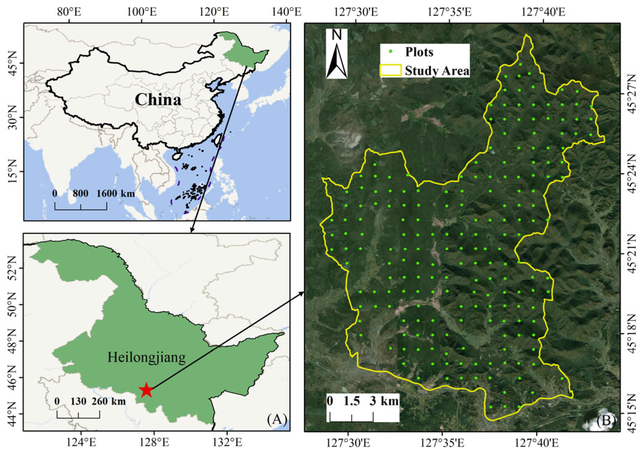
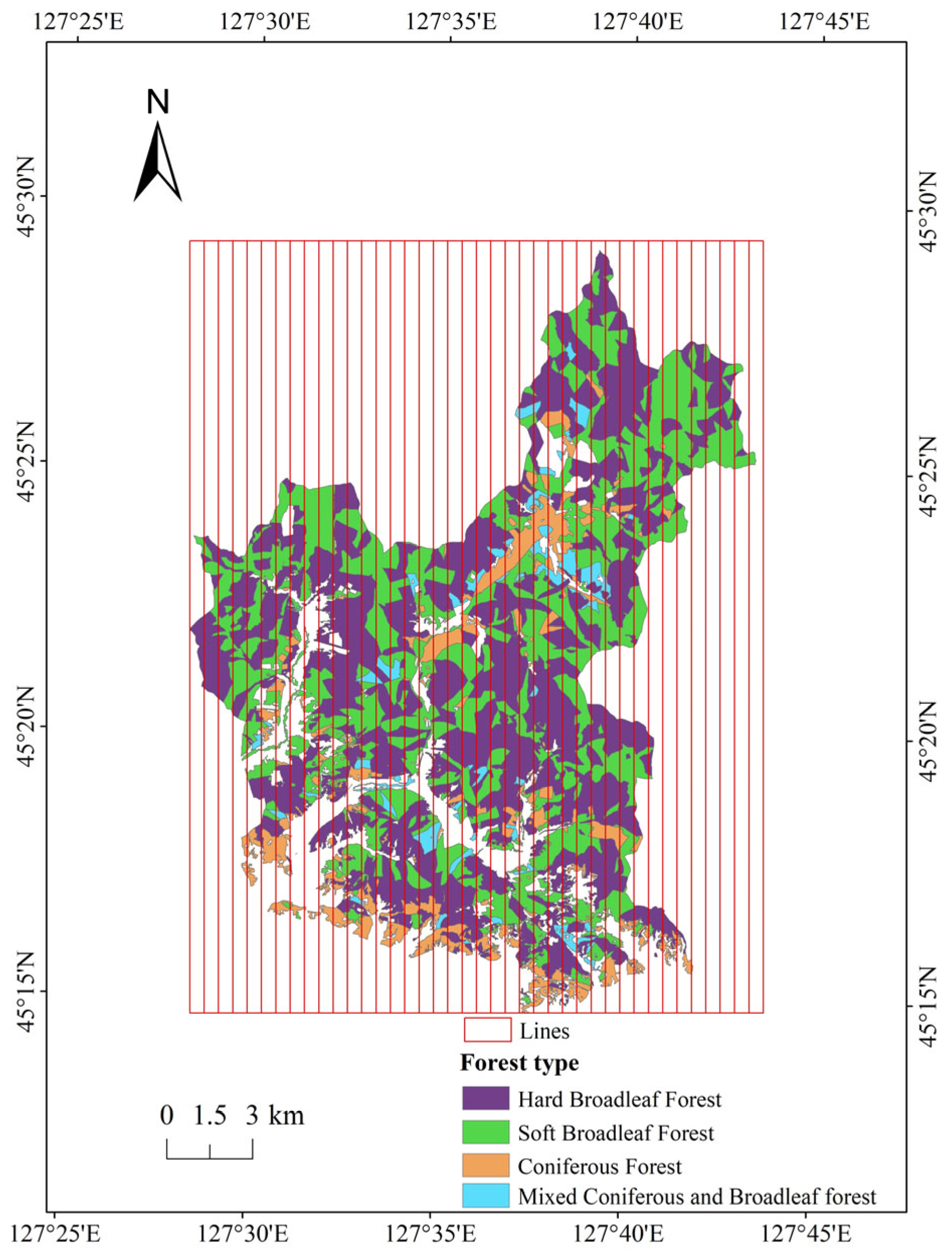
2.1. Study Area

Maoshan Forest Farm (45°14′–45°29′ N, 127°29′–127°44′ E) is a typical natural secondary forest in Northeast China and covers 26,496 ha (Figure 1). The terrain of the forest area is gradual and gentle from north to south, with an average elevation of around 300 m [35]. It is located in Harbin City, Heilongjiang Province, China, where the soil is dominated by dark brown loam, and which has a mid-temperate continental monsoon climate, with an average annual temperature of 2.8 °C and an average annual precipitation of about 723 mm. The original dominant community in this area was a Korean pine (Pinus koraiensis) forest, which has evolved into a typical natural secondary forest after years of human disturbance. The forest vegetation is dominated by broad-leaved trees, such as Mongolian oak (Quercus mongolica), walnut (Juglans mandshurica), Manchurian ash (Fraxinus manchuria), and white birch (Betula platyphylla), accompanied by a small number of coniferous trees such as Korean pine and larch (Larix olgensis).

2.2. Field and Multi-Sensor Data Acquisition

The field investigation was conducted in August 2016 using systematic sampling (sampling interval of 1 km). In total, 197 plots with an area of 0.06 ha (24.5 m × 24.5 m) were measured. Trees with a diameter at breast height (DBH) greater than 5 cm in the plots were measured, including species and status, and the center of each plot was recorded using the global positioning system receiver (positioning accuracy of ±5 m). Field plot volume was calculated according to the tree volume table of the National Forestry and Grassland Administration of China (https://www.forestry.gov.cn/ (accessed on 5 August 2020)) combined with the measured DBH, and the plot volume was calculated according to the average volume per unit area within each field plot in cubic meters per hectare (m3/ha). The 197 plots were randomly allocated into 137 plots for modeling and 60 plots for independent validation. The statistical data for the field plot is presented in Table 1. In addition, the forest type of the whole forest was investigated and counted, and mainly divided into hard broadleaf forests, soft broadleaf forests, coniferous forests, and mixed coniferous and broadleaf forests.
The LiDAR and hyperspectral data were collected in September 2015 using the LiCHy airborne observation system of the Chinese Academy of Forestry (CAF), which was equipped on a fixed-wing aircraft [36]. The flight speed was approximately 65 m/s and the altitude was 1200 m above the ground. The scanning coverage area was approximately 360 km2. LiDAR data were acquired using a Riegl LMS-Q680i sensor with a wavelength of 1550 nm, beam divergence of 0.5 mrad, pulse length of 3 ns, and scanning angle of ±30° (perpendicular to flight direction). The average density of point clouds in the plots was 8 pts/m2. The hyperspectral data were collected using the AISA Eagle II sensor. The hyperspectral image had 64 bands that spanned the spectral range from 380 to 1000 nm, including 39 bands between the visible and red-edge regions and 25 bands in the near-infrared. It had a spatial resolution of 1.5 m and a spectral resolution of 3.3 nm. In addition, the DEM data from ALOS (derived from PALSAR data during 2006 to 2011) were downloaded from the Japan Aerospace Exploration Agency.

2.3. Methods

2.3.1. Remote Sensing Data Processing
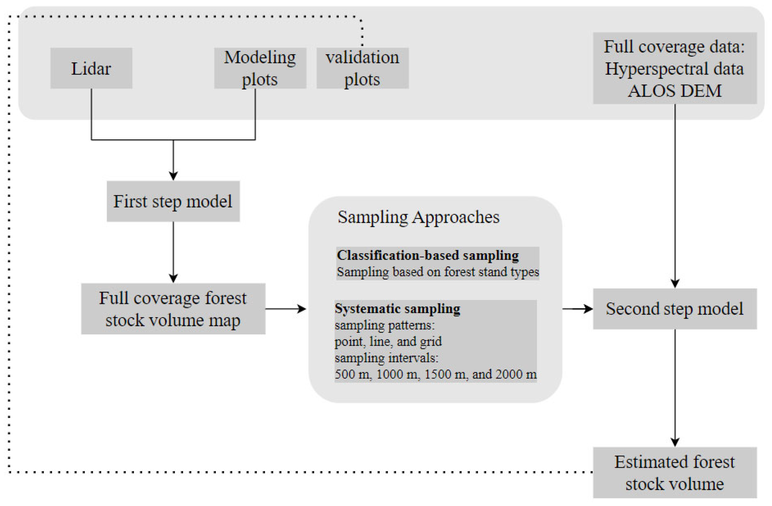
Preprocessing of LiDAR data involved first identifying and removing noise points (isolated points, low points, etc.). Then, the point cloud classification (ground and vegetation points) was performed using a modified progressive triangular irregular network (TIN) densification algorithm, and the digital terrain model (DTM) was generated from the ground points using the kriging method with a spatial resolution of 1 m [37]. Finally, the elevation values of the original point cloud were subtracted from the corresponding nearest DTM values to obtain the height above ground for each point. The LiDAR data preprocessing was performed using LiDAR360 V5.0 software [38]. To eliminate the influence of low shrubs, the height threshold was set to 2 m. Point cloud features that could reflect the internal structure and radiation information of the forest were extracted from LiDAR data, which mainly included 5 categories: (1) height features, (2) density features, (3) intensity features, (4) canopy features, and (5) topographic features. Detailed information on LiDAR features is listed in Table 2.
Hyperspectral data preprocessing was performed using FLAASH atmospheric correction (ENVI; version 5.6) to remove atmospheric and illumination effects to obtain surface reflectance data. For hyperspectral images, we extracted 64 original bands ( B λ , where λ is the center wavelength in nm) and 14 spectral vegetation indices, and these features mainly explored the potential correlation between spectral bands and vegetation properties: the visible band (380–690 nm) is mainly related to vegetation color (i.e., pigments); the red-edge band (690–760 nm) is sensitive to chlorophyll changes; the near-infrared band (760–1000 nm) reflects the scattering of radiation by the vegetation canopy. The spectral features at the pixel level were first extracted, and then the pixel average within the plot was counted to obtain the spectral features at the plot level. In addition, topographic features were extracted from the ALOS DEM (including DEM, slope, and aspect). The complete description of the vegetation index is shown in Table 3. All extracted remote sensing features were resampled to 24.5 m utilizing the nearest-neighbor algorithm to match the plot size.

2.3.2. Overview

This study is mainly divided into two steps (Figure 2). As the first step, the forest stock volume of the entire region was modeled and estimated based on ground-measured plots and full-coverage LiDAR data. In the second step, the influence of different sampling approaches was explored. By using systematic sampling (point, line, grid) and classification-based sampling to select samples, the forest stock volume estimated in the first step was used as reference data, combined with remote sensing features (spectral and topographic features) for modeling, to evaluate whether a two-step forest stock volume model constructed using a small number of LiDAR samples can achieve or approximate the accuracy of using full-coverage LiDAR data. The study also aims to determine the impact of sampling approaches on the accuracy of forest stock volume estimation and find an optimal scheme for collecting LiDAR samples (a trade-off between cost and accuracy). The accuracy of the forest stock volume estimation was verified by independent plots, utilizing the root mean square error (RMSE, in m3/ha) and mean error (BIAS, in m3/ha) computed from observed and predicted data to evaluate the accuracy of different sampling approaches.

2.3.3. Modeling and Feature Selection

This study used a multiple linear model (LM) to explore the relationship between forest stock volume and multi-source remote sensing features.
V = u 0 + j = 1 p u j X i j + ε i   ( i = 1 , , n )
where u 0 is the intercept, u j is the model coefficient, X i j is the remote sensing feature, and ε i represents the error term. The LM model was used in both steps of the model in this study. In the first-step model, the stand volume of the 137 plots was used as the explanatory variable, LiDAR features were used as the explanatory variables, and a logarithmic transformation was used to reduce the heteroscedasticity [50]. In the second-step model, the estimated volume from LiDAR was the dependent variable, and the model was constructed by combining spectral and topographic features.
When applying multiple linear models, the commonly used feature selection methods mainly include forward selection, backward selection, and stepwise selection. Among these, stepwise multiple linear regression (SMLR) is the most widely used [51]. SMLR combines the advantages of the forward and backward selection methods, where the features are ranked in descending order of their contribution to the regression equation and introduced sequentially into the regression model at a set F-test level. If a factor that has been selected becomes no longer significant due to a decrease in importance caused by the influence of a newly added factor, it is deleted from the regression equation to ensure the value of each feature left in the model, and features are introduced or deleted according to this pattern until there are no more new features to be introduced or deleted, and the regression model thus obtained is considered to be the optimal regression model. All models in this study were filtered for features using the SMLR method. In addition, the second-step models used forest stock volumes estimated from full-coverage LiDAR data with remote sensing features (spectral and topographic features) for stepwise filtering to ensure that all of the second-step models had the same features.

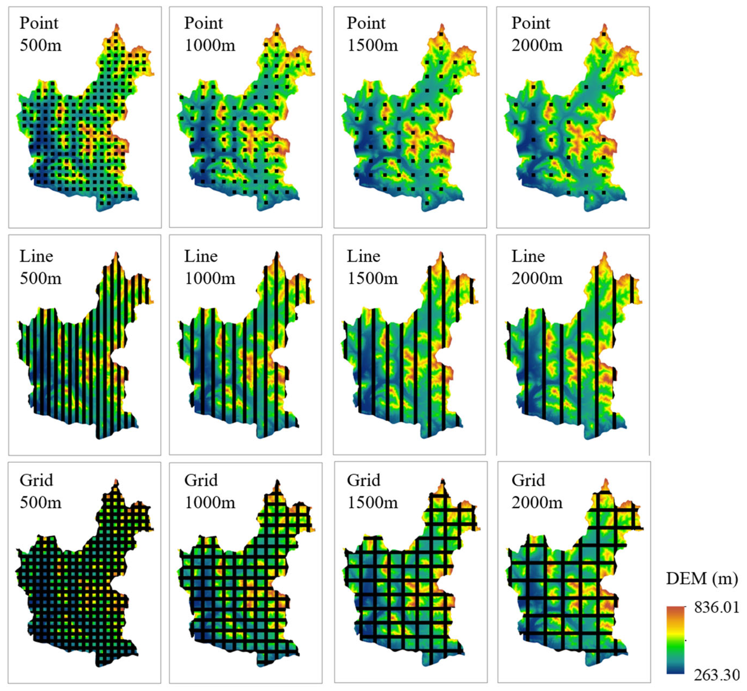
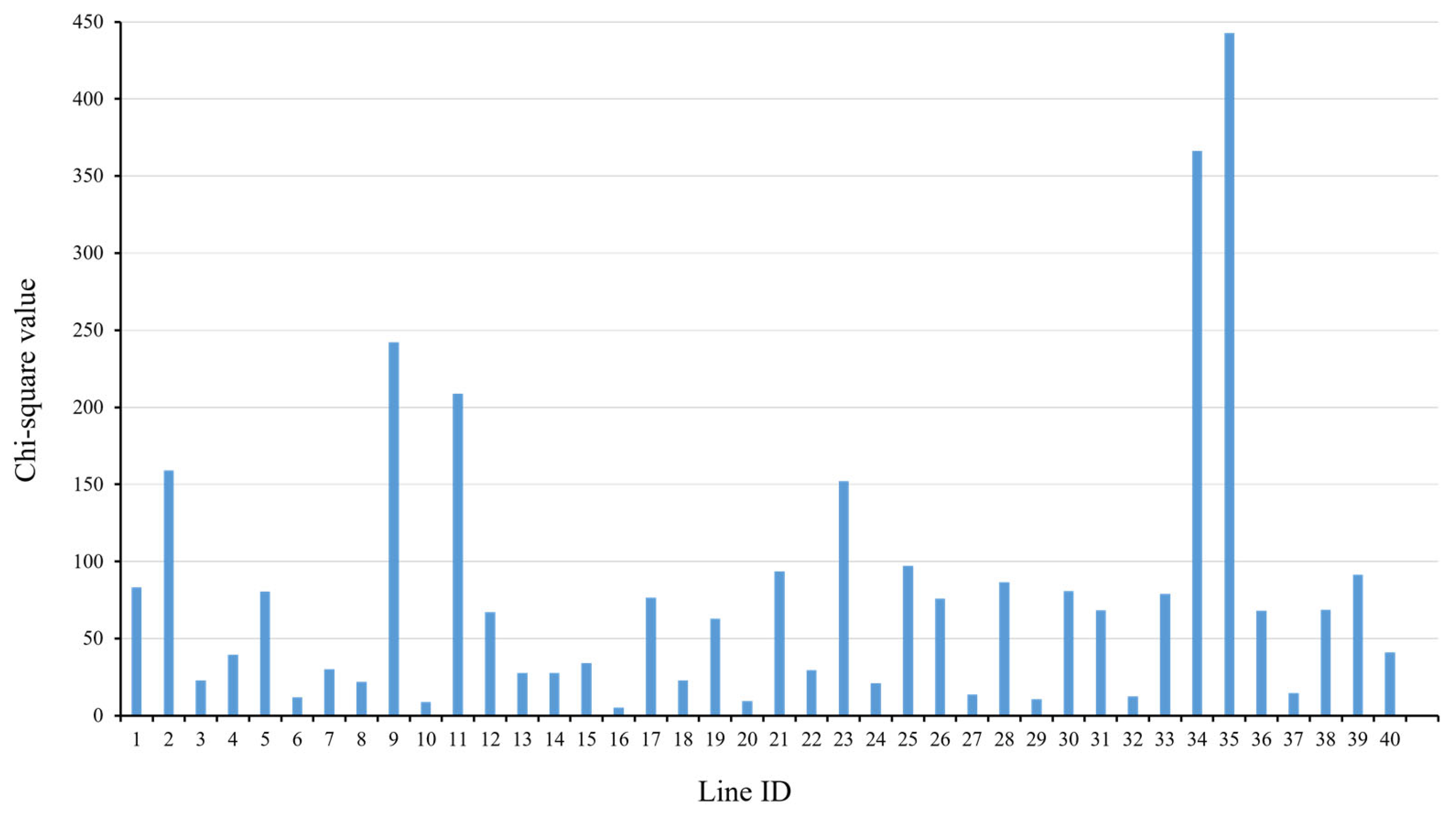
2.3.4. Systematic Sampling

The sampling approaches of this study include systematic sampling and classification-based sampling. Systematic sampling, also known as equidistant sampling or mechanical sampling, is a sampling method in which samples are taken at pre-specified intervals after determining the starting point. We used three sampling patterns (point, line, and grid) and four sampling intervals (500 m, 1000 m, 1500 m, and 2000 m) for systematic sampling to obtain 12 systematic LiDAR samples (Figure 3). Considering the aircraft line characteristics, we adopted 500 × 500 m as the basic sampling unit.

2.3.5. Sampling Based on Forest Stand Types

Classification-based sampling differs from systematic sampling in that, instead of sampling at predetermined intervals, samples are selected from forest types that best match the study area. There are many ways to explore the relationship between samples and population. The chi-square goodness-of-fit test is a statistical hypothesis test used to determine whether a variable is likely to come from a specified distribution, and it is often used to assess whether sample data are representative of the population [34]. The principle is to calculate the difference between the observed frequencies obtained from sampling and the theoretical frequencies (i.e., expected frequencies) in the original hypothetical distribution; if the observed and theoretical frequencies are closer, it means that the degree of conformity is better, i.e., the goodness of fit is better.
χ 2 = i = 1 k O i T i 2 T i ,     T i = n P i
where O i denotes the frequency of observations, T i denotes the theoretical frequency, P i denotes the percentage of group i in the theoretical distribution, n denotes the total number of observations, and k denotes the number of groups. A smaller χ 2 value indicates no significant difference between the samples and the population, whereas a larger value indicates a greater difference between the sample and the population. We divided the entire study area into 40 lines (500 m apart), O i being the distribution of forest types in each line and T i the overall distribution of forest types in the study area, calculated the χ 2 value of each line, and selected the line with the smaller χ 2 value to represent the entire study area.

2.3.6. Accuracy Evaluation

We used 10-fold cross-validation to evaluate the first-step model’s performance by the coefficient of determination (R2) and root mean square error (RMSE). The second-step model was evaluated for accuracy using measured data from 60 independent plots, and the root mean square error (RMSE, in m3/ha) and mean error (BIAS, in m3/ha) calculated using observed and predicted data were used to evaluate the accuracy of different sampling approaches.
R 2 = 1 i = 1 n ( y i y ^ i ) 2 i = 1 n ( y i y ¯ ) 2
R M S E = i = 1 n ( y i y ^ i ) 2 n
B I A S = i = 1 n ( y i y ^ i ) n
where y i denotes measured volume, y ^ i denotes predicted volume, and n denotes the number of validation plots.

3. Results

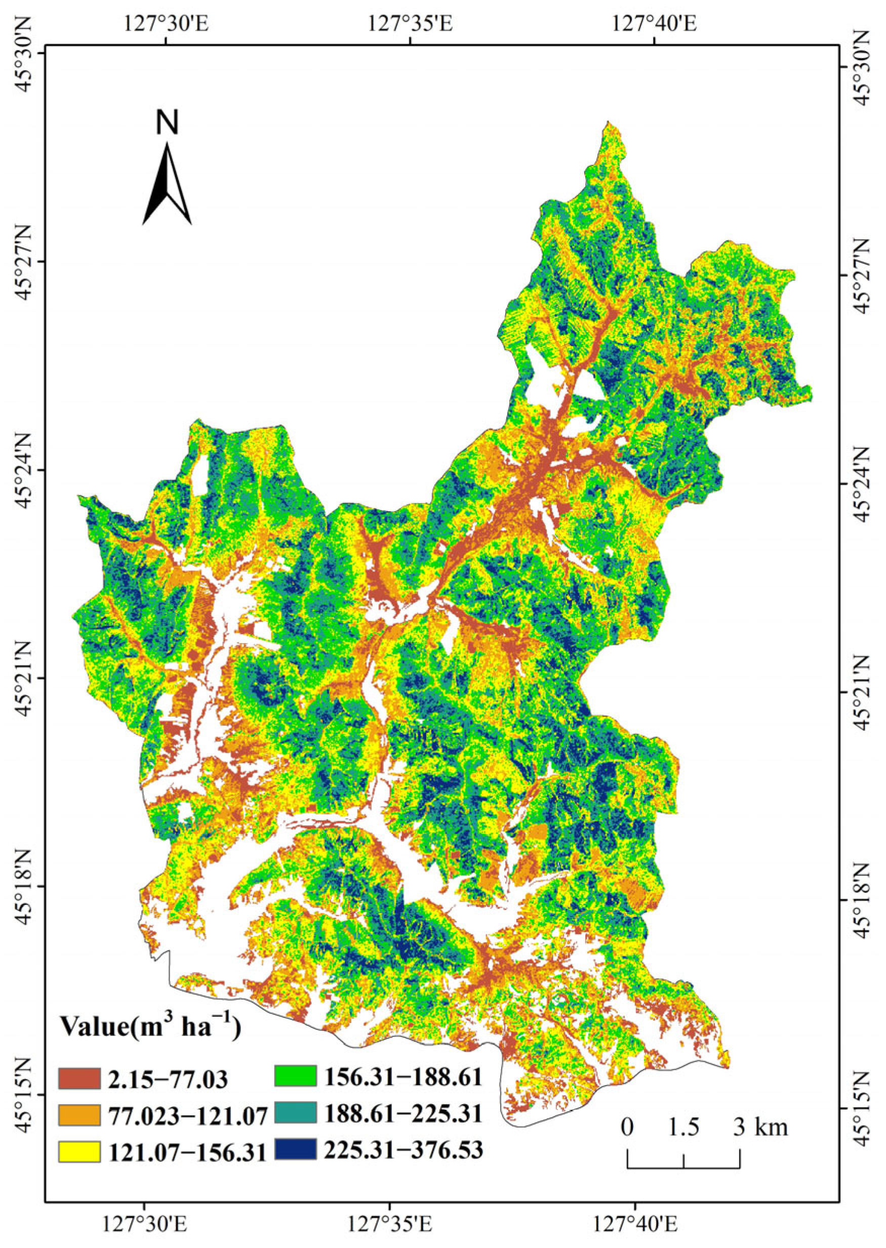
3.1. Full-Coverage LiDAR Forest Stock Volume Estimation

The LM model was constructed based on 137 plots of measured data with LiDAR features and validated with 10-fold cross-validation. The regression equation is shown in Equation (6), and four LiDAR features were obtained using the stepwise regression method: Hmean, slope, aspect, and I01. The R2 value was 0.43 and the RMSE was 49.91 m3/ha. The scatterplot of the forest stock volume model constructed based on the full-coverage LiDAR is presented in Figure 4.
V = e 3.20 + 1.18 × H m e a n + 0.19 × S l o p e + 0.12 × A s p e c t 1.07 × I 01
The measured values of forest stock volume ranged from 34.01 to 468.99 m3/ha, mainly below 250 m3/ha, with a mean and standard deviation of 175.32 and 64.76 m3/ha, respectively. The range of forest stock volume values estimated for the whole region using the LM model was 2.15–376.53 m3/ha, with a mean and standard deviation of 152.66 and 53.14 m3/ha, respectively. Overall, the forest stock volume distribution obtained from the full-coverage LiDAR-based estimation was similar to the measured values (Figure 5).

3.2. Systematic Sampling for Forest Stock Volume Estimation

We used the forest stock volume obtained from the first-step estimation as the reference data, and used a small amount of LiDAR as an intermediate sample to construct a two-step volume model to explore whether it could reach or approach the accuracy of using full-coverage LiDAR data. Eight variables were obtained by stepwise regression filtering (slope, DEM, SR, aspect, CRI1, PRI, ARI2, and B657), which were used to construct regression models for multiple sampling approaches, and 60 independent validation data plots were used to evaluate the accuracy of the second-step models, and the number of pixels used in different sampling approaches was also counted (Table 4).
Among the 12 systematic sampling methods, line sampling with a sampling interval of 1000 m had the highest accuracy, with an RMSE of 55.81 m3/ha and a BIAS of 21.55 m3/ha. In the sampling intervals of 500 m, 1000 m, and 1500 m, line sampling had the lowest values for the RMSE and BIAS, and was better than point and grid sampling. The RMSE of the models with different systematic sampling methods ranged from 55.81 to 57.42 m3/ha. Compared to the full-coverage LiDAR model (RMSE = 49.91 m3/ha), the RMSE of the line sampling with the highest accuracy increased by 11.8%. Overall, line sampling performed well in terms of accuracy and was consistent with the characteristics of aircraft routes and easier to plan, which makes it easier to apply in reality. Therefore, we chose to use line sampling for further analysis.

3.3. Classification-Based Sampling for Forest Stock Volume Estimation

For the classification-based sampling approach, we used 500 m as the sampling interval, and the entire study area was divided into 40 lines, with the forest types consisting of four main forest types: hard broadleaf forests, soft broadleaf forests, coniferous forests, and mixed coniferous and broadleaf forests (Figure 6). To select the most representative lines to represent the entire study area, we calculated the chi-square value for each line by combining the proportion of forest types within each line and across the region. Lines with smaller chi-square values imply that their forest-type distribution is closer to the entire study area. We selected eight lines (6, 10, 16, 20, 27, 29, 32, and 37) as LiDAR samples depending on the results in Figure 7.
Forest stock volume in eight lines was used to construct a regression model with eight remote sensing features (five spectral features and three topographic features). The model results are presented in Table 5. The RMSE was 55.56 (<55.81 m3/ha) and the BIAS was 20.68 (<21.55 m3/ha). The classification-based sampling estimation results outperformed the systematic sampling.

4. Discussion

The goal of this study was to explore the use of a small number of LiDAR samples as intermediate data to link field data with full-coverage multi-sensor imagery for reliable wall-to-wall forest stock volume mapping. Specifically, we aimed to evaluate the robustness of the sampling technique and find an optimal scheme for collecting LiDAR samples that allows an accurate estimation of forest stock volume without relying on full-coverage LiDAR data and without a significant reduction in accuracy.
We compared the modeling accuracies of systematic sampling and classification-based sampling with that of full-coverage LiDAR. The sampling-based modeling accuracy was found to decrease by 11.3%–15.0%, with the most accurate being the classification-based sampling approach, which accounted for 22.64% of the total pixels, and did not account for more pixels the higher the modeling accuracy (the grid sampling with 500 m intervals accounted for 74.65% of the total pixels, but the RMSE increased by 15.0%). This is different from the findings of Tusi et al., whose study showed that model accuracy increased with the number of pixels, possibly because their study area was simpler and fewer sampling methods were explored [32]. The conclusion of this study suggests that classification-based sampling is more representative of the population.
The study area was a natural secondary forest, and its complex stand conditions, such as vegetation overlap between stands, uneven canopy cover, and dense near-surface scrub, may have led to difficulties in capturing stand structure and vegetation distribution from LiDAR data, which affected the accurate estimation of forest stock volume by the first-step model [22]. In addition, we used the forest stock volume estimated by LiDAR as a reference value for secondary modeling, which introduced additional uncertainty [52]. Compared with the volume values estimated in the first step, the volume values estimated by the regression model in the second step have a narrower range, which indicates the existence of a saturation effect. This saturation effect may be influenced by limitations in the spatial and temporal resolution of the optical images, the diversity of forest types, and the complexity of the forest structure [53]. The saturation effect limits the accuracy and validity of forest stock volume estimation from optical images, which is a factor that needs to be explored and considered in future research.
Several studies have explored LiDAR sampling approaches, among which the line sampling approach has been widely utilized. Line sampling fits the characteristics of aircraft routes, which makes it a good balance between practical applications, cost-effectiveness, and accuracy [31]. As pointed out by Chen and Hay, different intervals of the LiDAR sample lines led to different results, which is consistent with our results (Table 5). However, the difference in model accuracy between the different sampling methods in this study was not significant, which may be due to the lower accuracy of the first-step model [54]. Subsequent consideration should be paid to improving the first-step model’s accuracy to reduce error transmission.
We used airborne hyperspectral imagery for the second step of modeling, which has a wider spectral range and more detailed features than multispectral imagery and explores forest vegetation information (e.g., structure, pigmentation, water content, etc.), which helps to improve model performance [55]. Regarding the results of model feature filtering in the second step, there were mainly five spectral features and three topographic features, of which the spectral features were the simple ratio index (SR), the photochemical reflectance index (PRI), and the vegetation indices related to carotenoids and anthocyanins (CRI1 and ARI2), which mainly involved the green band (510–570 nm), the red-edge band (700 nm), and the near-infrared band (900 nm), which is consistent with previous studies showing that these biochemical traits covary with forest canopy structure, which is important for estimating forest stock volume [22]. In addition, topographic relief may lead to differences in vegetation distribution, and joint analysis of hyperspectral data and DEM can reveal this relationship. We used airborne hyperspectral imagery rather than hyperspectral satellite imagery with the intention of exploring the potential of hyperspectral data in estimating forest parameters, and the hyperspectral features obtained from the filtering in this study can also be transferred to other multispectral or hyperspectral imagery, and in addition, as resources such as the Zhuhai-1 hyperspectral satellite imagery can be downloaded and utilized after application, we believe that hyperspectral satellite imagery will certainly be more open and gain wider application in the future [56].
Our study used forest-type data provided by the forest farm for sample selection. For the portability of the method, the study area can be categorized in advance based on optical imagery to obtain regionally representative LiDAR lines, and Chen et al. showed that more accurate results can be obtained by modeling different forest types separately [57]. A classification-based sampling method fully considers the diversity of forest types and can better capture the characteristics of, and changes in, different types of forests, especially when there are significant differences in forest types. The sampling method provides a way in which we can reduce the acquisition of LiDAR data without significantly reducing accuracy. It is noted that additional analytical work is required to perform the classification.

5. Conclusions

In this study, we explored a sampling framework that uses a small number of LiDAR data samples as intermediate data to link measured forest stock volume and full-coverage multi-source remote sensing data for efficient and reliable full-coverage forest stock volume estimation. We compared two sampling approaches, systematic sampling and classification-based sampling, and the results showed that the classification-based LiDAR sampling has a higher modeling accuracy (RMSE = 55.56 m3/ha, BIAS = 20.68 m3/ha). In addition, different sampling intervals and sampling methods can affect the results of systematic sampling. It is not as if the higher the number of pixels, the higher the accuracy of the model; the samples selected based on the classification are more representative of the overall picture. The study site covers most of the tree species and forest types in Northeast China and is transferable. In the future, further experiments can be conducted in other forest types and climatic zones, and the mechanism of error transfer can be considered to understand how errors accumulate at different modeling stages. Given the results of the study, we recommend a classification-based sampling approach as the basis for LiDAR sample collection in applications. This study contributes to the exploration of more cost-effective airborne LiDAR data acquisition schemes.

Author Contributions

Conceptualization, M.L. and B.W.; methodology, Y.Q.; software, J.L.; validation, J.S. and J.L.; formal analysis, J.S.; investigation, L.M.; resources, M.L.; data curation, B.W.; writing—original draft preparation, J.L.; writing—review and editing, Y.Q.; visualization, J.S.; supervision, Y.Q.; project administration, B.W.; funding acquisition, M.L. All authors have read and agreed to the published version of the manuscript.

Funding

This research was funded by the National Key Research and Development Program of China (grant number 2020YFC1511603-1); Fundamental Research Funds for the Central Universities (grant number 2572022DT03); carbon neutrality special scientific foundation project (grant number HFW220100054); and the China Longjiang Forest Industry Group Subsidized scientific and technological projects (grant number HFW230100074).

Data Availability Statement

Due to the nature of this research, participants of this study did not agree for their data to be shared publicly, so supporting data is not available.

Acknowledgments

The authors would like to thank the faculty and students of the Department of Forest Management, Northeast Forestry University (NEFU), China, who collected and provided the data for this study.

Conflicts of Interest

The authors declare no conflict of interest.

References

  1. Pan, Y.D.; Birdsey, R.A.; Fang, J.Y.; Houghton, R.; Kauppi, P.E.; Kurz, W.A.; Phillips, O.L.; Shvidenko, A.; Lewis, S.L.; Canadell, J.G.; et al. A Large and Persistent Carbon Sink in the World’s Forests. Science 2011, 333, 988–993. [Google Scholar] [CrossRef]
  2. Condés, S.; McRoberts, R.E. Updating national forest inventory estimates of growing stock volume using hybrid inference. For. Ecol. Manag. 2017, 400, 48–57. [Google Scholar] [CrossRef]
  3. Liang, X.L.; Hyyppä, J.; Kaartinen, H.; Lehtomäki, M.; Pyörälä, J.; Pfeifer, N.; Holopainen, M.; Brolly, G.; Pirotti, F.; Hackenberg, J.; et al. International benchmarking of terrestrial laser scanning approaches for forest inventories. ISPRS J. Photogramm. 2018, 144, 137–179. [Google Scholar] [CrossRef]
  4. Boisvenue, C.; Smiley, B.P.; White, J.C.; Kurz, W.A.; Wulder, M.A. Integration of Landsat time series and field plots for forest productivity estimates in decision support models. For. Ecol. Manag. 2016, 376, 284–297. [Google Scholar] [CrossRef]
  5. Hao, Y.S.; Widagdo, F.R.A.; Liu, X.; Quan, Y.; Dong, L.H.; Li, F.R. Individual Tree Diameter Estimation in Small-Scale Forest Inventory Using UAV Laser Scanning. Remote Sens. 2021, 13, 24. [Google Scholar] [CrossRef]
  6. Tomppo, E.; Olsson, H.; Ståhl, G.; Nilsson, M.; Hagner, O.; Katila, M. Combining national forest inventory field plots and remote sensing data for forest databases. Remote Sens. Environ. 2008, 112, 1982–1999. [Google Scholar] [CrossRef]
  7. Saarela, S.; Grafström, A.; Ståhl, G.; Kangas, A.; Holopainen, M.; Tuominen, S.; Nordkvist, K.; Hyyppä, J. Model-assisted estimation of growing stock volume using different combinations of LiDAR and Landsat data as auxiliary information. Remote Sens. Environ. 2015, 158, 431–440. [Google Scholar] [CrossRef]
  8. Kilpeläinen, P.; Tokola, T. Gain to be achieved from stand delineation in LANDSAT TM image-based estimates of stand volume. For. Ecol. Manag. 1999, 124, 105–111. [Google Scholar] [CrossRef]
  9. Chrysafis, I.; Mallinis, G.; Tsakiri, M.; Patias, P. Evaluation of single-date and multi-seasonal spatial and spectral information of Sentinel-2 imagery to assess growing stock volume of a Mediterranean forest. Int. J. Appl. Earth Obs. 2019, 77, 1–14. [Google Scholar] [CrossRef]
  10. Long, J.P.; Lin, H.; Wang, G.X.; Sun, H.; Yan, E.P. Mapping Growing Stem Volume of Chinese Fir Plantation Using a Saturation-based Multivariate Method and Quad-polarimetric SAR Images. Remote Sens. 2019, 11, 1872. [Google Scholar] [CrossRef]
  11. Chen, L.; Ren, C.Y.; Zhang, B.; Wang, Z.M. Multi-Sensor Prediction of Stand Volume by a Hybrid Model of Support Vector Machine for Regression Kriging. Forests 2020, 11, 296. [Google Scholar] [CrossRef]
  12. Santi, E.; Paloscia, S.; Pettinato, S.; Chirici, G.; Mura, M.; Maselli, F. Application of Neural Networks for the retrieval of forest woody volume from SAR multifrequency data at L and C bands. Eur. J. Remote Sens. 2015, 48, 673–687. [Google Scholar] [CrossRef]
  13. Cartus, O.; Kellndorfer, J.; Rombach, M.; Walker, W. Mapping Canopy Height and Growing Stock Volume Using Airborne Lidar, ALOS PALSAR and Landsat ETM. Remote Sens. 2012, 4, 3320–3345. [Google Scholar] [CrossRef]
  14. Puliti, S.; Saarela, S.; Gobakken, T.; Ståhl, G.; Næsset, E. Combining UAV and Sentinel-2 auxiliary data for forest growing stock volume estimation through hierarchical model-based inference. Remote Sens. Environ. 2018, 204, 485–497. [Google Scholar] [CrossRef]
  15. Chen, L.; Ren, C.Y.; Zhang, B.; Wang, Z.M.; Liu, M.Y.; Man, W.D.; Liu, J.F. Improved estimation of forest stand volume by the integration of GEDI LiDAR data and multi-sensor imagery in the Changbai Mountains Mixed forests Ecoregion (CMMFE), northeast China. Int. J. Appl. Earth Obs. 2021, 100, 102326. [Google Scholar] [CrossRef]
  16. Gong, P.; Pu, R.L.; Biging, G.S.; Larrieu, M.R. Estimation of forest leaf area index using vegetation indices derived from Hyperion hyperspectral data. IEEE T Geosci. Remote 2003, 41, 1355–1362. [Google Scholar] [CrossRef]
  17. Psomas, A.; Kneubühler, M.; Huber, S.; Itten, K.; Zimmermann, N.E. Hyperspectral remote sensing for estimating aboveground biomass and for exploring species richness patterns of grassland habitats. Int. J. Remote Sens. 2011, 32, 9007–9031. [Google Scholar] [CrossRef]
  18. Roth, K.L.; Roberts, D.A.; Dennison, P.E.; Peterson, S.H.; Alonzo, M. The impact of spatial resolution on the classification of plant species and functional types within imaging spectrometer data. Remote Sens. Environ. 2015, 171, 45–57. [Google Scholar] [CrossRef]
  19. Quan, Y.; Li, M.Z.; Hao, Y.S.; Liu, J.Y.; Wang, B. Tree species classification in a typical natural secondary forest using UAV-borne LiDAR and hyperspectral data. Gisci Remote Sens. 2023, 60, 2171706. [Google Scholar] [CrossRef]
  20. Wan, L.M.; Lin, Y.Y.; Zhang, H.S.; Wang, F.; Liu, M.F.; Lin, H. GF-5 Hyperspectral Data for Species Mapping of Mangrove in Mai Po, Hong Kong. Remote Sens. 2020, 12, 656. [Google Scholar] [CrossRef]
  21. Kandare, K.; Dalponte, M.; Orka, H.O.; Frizzera, L.; Naesset, E. Prediction of Species-Specific Volume Using Different Inventory Approaches by Fusing Airborne Laser Scanning and Hyperspectral Data. Remote Sens. 2017, 9, 400. [Google Scholar] [CrossRef]
  22. De Almeida, C.T.; Galvao, L.S.; Aragao, L.E.D.E.; Ometto, J.P.H.B.; Jacon, A.D.; Pereira, F.R.D.; Sato, L.Y.; Lopes, A.P.; Graça, P.M.L.D.; Silva, C.V.D.; et al. Combining LiDAR and hyperspectral data for aboveground biomass modeling in the Brazilian Amazon using different regression algorithms. Remote Sens. Environ. 2019, 232, 111323. [Google Scholar] [CrossRef]
  23. Fassnacht, F.E.; Hartig, F.; Latifi, H.; Berger, C.; Hernández, J.; Corvalán, P.; Koch, B. Importance of sample size, data type and prediction method for remote sensing-based estimations of aboveground forest biomass. Remote Sens. Environ. 2014, 154, 102–114. [Google Scholar] [CrossRef]
  24. Koch, B. Status and future of laser scanning, synthetic aperture radar and hyperspectral remote sensing data for forest biomass assessment. ISPRS J. Photogramm. 2010, 65, 581–590. [Google Scholar] [CrossRef]
  25. Chirici, G.; Giannetti, F.; McRoberts, R.E.; Travaglini, D.; Pecchi, M.; Maselli, F.; Chiesi, M.; Corona, P. Wall-to-wall spatial prediction of growing stock volume based on Italian National Forest Inventory plots and remotely sensed data. Int. J. Appl. Earth Obs. 2020, 84, 101959. [Google Scholar] [CrossRef]
  26. De Souza, G.S.A.; Soares, V.P.; Leite, H.G.; Gleriani, J.M.; do Amaral, C.H.; Ferraz, A.S.; Silveira, M.V.D.; dos Santos, J.F.C.; Velloso, S.G.S.; Domingues, G.F.; et al. Multi-sensor prediction of stand volume: A support vector approach. ISPRS J. Photogramm. 2019, 156, 135–146. [Google Scholar] [CrossRef]
  27. Li, S.Q.; Quackenbush, L.J.; Im, J. Airborne Lidar Sampling Strategies to Enhance Forest Aboveground Biomass Estimation from Landsat Imagery. Remote Sens. 2019, 11, 1906. [Google Scholar] [CrossRef]
  28. Matasci, G.; Hermosilla, T.; Wulder, M.A.; White, J.C.; Coops, N.C.; Hobart, G.W.; Zald, H.S.J. Large-area mapping of Canadian boreal forest cover, height, biomass and other structural attributes using Landsat composites and lidar plots. Remote Sens. Environ. 2018, 209, 90–106. [Google Scholar] [CrossRef]
  29. Li, W.; Niu, Z.; Shang, R.; Qin, Y.C.; Wang, L.; Chen, H.Y. High-resolution mapping of forest canopy height using machine learning by coupling ICESat-2 LiDAR with Sentinel-1, Sentinel-2 and Landsat-8 data. Int. J. Appl. Earth Obs. 2020, 92, 102163. [Google Scholar] [CrossRef]
  30. Rahlf, J.; Breidenbach, J.; Solberg, S.; Næsset, E.; Astrup, R. Comparison of four types of 3D data for timber volume estimation. Remote Sens. Environ. 2014, 155, 325–333. [Google Scholar] [CrossRef]
  31. Wulder, M.A.; White, J.C.; Nelson, R.F.; Næsset, E.; Orka, H.O.; Coops, N.C.; Hilker, T.; Bater, C.W.; Gobakken, T. Lidar sampling for large-area forest characterization: A review. Remote Sens. Environ. 2012, 121, 196–209. [Google Scholar] [CrossRef]
  32. Tsui, O.W.; Coops, N.C.; Wulder, M.A.; Marshall, P.L. Integrating airborne LiDAR and space-borne radar via multivariate kriging to estimate above-ground biomass. Remote Sens. Environ. 2013, 139, 340–352. [Google Scholar] [CrossRef]
  33. Hudak, A.T.; Lefsky, M.A.; Cohen, W.B.; Berterretche, M. Integration of lidar and Landsat ETM+ data for estimating and mapping forest canopy height. Remote Sens. Environ. 2002, 82, 397–416. [Google Scholar] [CrossRef]
  34. Chen, G.; Hay, G.J. An airborne lidar sampling strategy to model forest canopy height from Quickbird imagery and GEOBIA. Remote Sens. Environ. 2011, 115, 1532–1542. [Google Scholar] [CrossRef]
  35. Quan, Y.; Li, M.Z.; Hao, Y.S.; Wang, B. Comparison and Evaluation of Different Pit-Filling Methods for Generating High Resolution Canopy Height Model Using UAV Laser Scanning Data. Remote Sens. 2021, 13, 2239. [Google Scholar] [CrossRef]
  36. Pang, Y.; Li, Z.; Ju, H.; Lu, H.; Jia, W.; Si, L.; Guo, Y.; Liu, Q.; Li, S.; Liu, L.; et al. LiCHy: The CAF’s LiDAR, CCD and Hyperspectral Integrated Airborne Observation System. Remote Sens. 2016, 8, 398. [Google Scholar] [CrossRef]
  37. Guo, Q.; Li, W.; Yu, H.; Alvarez, O. Effects of Topographic Variability and Lidar Sampling Density on Several DEM Interpolation Methods. Photogramm. Eng. Remote Sens. 2010, 76, 701–712. [Google Scholar] [CrossRef]
  38. Zhen, Z.; Yang, L.; Ma, Y.; Wei, Q.B.; Il Jin, H.; Zhao, Y.H. Upscaling aboveground biomass of larch (Henry) plantations from field to satellite measurements: A comparison of individual tree-based and area-based approaches. Gisci Remote Sens. 2022, 59, 722–743. [Google Scholar] [CrossRef]
  39. Gitelson, A.A.; Keydan, G.P.; Merzlyak, M.N. Three-band model for noninvasive estimation of chlorophyll, carotenoids, and anthocyanin contents in higher plant leaves. Geophys. Res. Lett. 2006, 33, L11402. [Google Scholar] [CrossRef]
  40. Huete, A.; Didan, K.; Miura, T.; Rodriguez, E.P.; Gao, X.; Ferreira, L.G. Overview of the radiometric and biophysical performance of the MODIS vegetation indices. Remote Sens. Environ. 2002, 83, 195–213. [Google Scholar] [CrossRef]
  41. Sims, D.A.; Gamon, J.A. Relationships between leaf pigment content and spectral reflectance across a wide range of species, leaf structures and developmental stages. Remote Sens. Environ. 2002, 81, 337–354. [Google Scholar] [CrossRef]
  42. Tucker, C.J. Red and photographic infrared linear combinations for monitoring vegetation. Remote Sens. Environ. 1979, 8, 127–150. [Google Scholar] [CrossRef]
  43. Evangelides, C.; Nobajas, A. Red-Edge Normalised Difference Vegetation Index (NDVI705) from Sentinel-2 imagery to assess post-fire regeneration. Remote Sens. Appl. Soc. Environ. 2020, 17, 100283. [Google Scholar] [CrossRef]
  44. Gamon, J.A.; Peñuelas, J.; Field, C.B. A narrow-waveband spectral index that tracks diurnal changes in photosynthetic efficiency. Remote Sens. Environ. 1992, 41, 35–44. [Google Scholar] [CrossRef]
  45. Merzlyak, M.N.; Gitelson, A.A.; Chivkunova, O.B.; Rakitin, V.Y.U. Non-destructive optical detection of pigment changes during leaf senescence and fruit ripening. Physiol. Plant. 2002, 106, 135–141. [Google Scholar] [CrossRef]
  46. Jordan, C.F. Derivation of Leaf-Area Index from Quality of Light on the Forest Floor. Ecology 1969, 50, 663–666. [Google Scholar] [CrossRef]
  47. You, W.Q.; Wang, Z.Y.; Lu, F.; Zhao, Y.S.; Lu, S. Spectral indices to assess the carotenoid/chlorophyll ratio from adaxial and abaxial leaf reflectance. Spectrosc. Lett. 2017, 50, 387–393. [Google Scholar] [CrossRef]
  48. Vogelmann, J.E.; Rock, B.N.; Moss, D.M. Red edge spectral measurements from sugar maple leaves. Int. J. Remote Sens. 2007, 14, 1563–1575. [Google Scholar] [CrossRef]
  49. Penuelas, J.; Pinol, J.; Ogaya, R.; Filella, I. Estimation of plant water concentration by the reflectance Water Index WI (R900/R970). Int. J. Remote Sens. 2010, 18, 2869–2875. [Google Scholar] [CrossRef]
  50. Dong, L.H.; Zhang, Y.; Zhang, Z.; Xie, L.F.; Li, F.R. Comparison of Tree Biomass Modeling Approaches for Larch (Henry) Trees in Northeast China. Forests 2020, 11, 202. [Google Scholar] [CrossRef]
  51. Yu, X.H.; Ge, H.L.; Lu, D.S.; Zhang, M.Z.; Lai, Z.X.; Yao, R.T. Comparative Study on Variable Selection Approaches in Establishment of Remote Sensing Model for Forest Biomass Estimation. Remote Sens. 2019, 11, 1437. [Google Scholar] [CrossRef]
  52. Skowronski, N.S.; Clark, K.L.; Gallagher, M.; Birdsey, R.A.; Hom, J.L. Airborne laser scanner-assisted estimation of aboveground biomass change in a temperate oak-pine forest. Remote Sens. Environ. 2014, 151, 166–174. [Google Scholar] [CrossRef]
  53. Zhao, P.P.; Lu, D.S.; Wang, G.X.; Wu, C.P.; Huang, Y.J.; Yu, S.Q. Examining Spectral Reflectance Saturation in Landsat Imagery and Corresponding Solutions to Improve Forest Aboveground Biomass Estimation. Remote Sens. 2016, 8, 469. [Google Scholar] [CrossRef]
  54. Hao, Y.S.; Widagdo, F.R.A.; Liu, X.; Quan, Y.; Liu, Z.G.; Dong, L.H.; Li, F.R. Estimation and calibration of stem diameter distribution using UAV laser scanning data: A case study for larch forests in Northeast China. Remote Sens. Environ. 2022, 268, 112769. [Google Scholar] [CrossRef]
  55. Zhou, K.; Cao, L.; Liu, H.; Zhang, Z.N.; Wang, G.B.; Cao, F.L. Estimation of volume resources for planted forests using an advanced LiDAR and hyperspectral remote sensing. Resour. Conserv. Recy 2022, 185, 106485. [Google Scholar] [CrossRef]
  56. Wang, D.Z.; Qiu, P.H.; Wan, B.; Cao, Z.X.; Zhang, Q.F. Mapping α- and β-diversity of mangrove forests with multispectral and hyperspectral images. Remote Sens. Environ. 2022, 275, 113021. [Google Scholar] [CrossRef]
  57. Chen, Q.; Laurin, G.V.; Battles, J.J.; Saah, D. Integration of airborne lidar and vegetation types derived from aerial photography for mapping aboveground live biomass. Remote Sens. Environ. 2012, 121, 108–117. [Google Scholar] [CrossRef]
Figure 1. The location of the study area (Maoshan Forest Farm). (A): The location of Harbin in Heilongjiang Province. (B): The locations of field plots in the study area from Google imagery (coordinate system: WGS 1984 UTM Zone 52N).
Forests 14 02453 g001
Figure 2. Overall workflow of the LiDAR sampling framework of forest stock volume estimation.
Forests 14 02453 g002
Figure 3. Spatial distribution of 12 systematic sampling-based LiDAR samples over the DEM.
Forests 14 02453 g003
Figure 4. Scatterplot of measured versus predicted volume values.
Forests 14 02453 g004
Figure 5. Spatial distribution of forest stock volume based on full-coverage LiDAR estimation. Non-forest areas are masked out.
Forests 14 02453 g005
Figure 6. Forest-type distribution and line delineation in the study area.
Forests 14 02453 g006
Figure 7. The chi-square value for each line in the study area. The X-axis represents the line ID and the Y-axis represents the chi-square value.
Forests 14 02453 g007
Table 1. Description of field plots volume divided into modeling and validation plots.
Plot GroupPlot
Number
Volume (m3/ha)
MeanMaxMinSD
Modeling137172.62468.9934.0166.91
Validation60181.49347.1154.3459.64
Total197175.32468.9934.0164.76
Table 2. List of LiDAR features derived from point cloud data. Calculation details are described by Zhen (2022) [38].
Metric TypeMetricsDescription
Height (38)Hmax, HmeanMaximum height, mean height
HVAR, HSD, HCVVariance of heights, standard deviation of heights, coefficient of variation of heights
HSK, HKSkewness of heights, kurtosis of heights
HIQInterquartile distance of percentile heights
H01, H05, H10, H20, H25, H30, H40, H50, H60, H70, H75, H80, H90, H95, H99Height percentiles. Point clouds are sorted by elevation. HX is the height of X% of the point clouds.
AIH01, AIH05, AIH10, AIH20, AIH25, AIH30, AIH40, AIH50, AIH60, AIH70, AIH75, AIH80, AIH90, AIH95, AIH99Cumulative height percentiles. Point clouds are sorted by elevation and the cumulative height of all points is calculated. AIHX is the cumulative height of X% of the point clouds.
Density (10)D01, D02, D03, D04, D05, D06, D07, D08, D09Canopy return density. Point clouds are divided into ten slices of the same interval from low to high elevation. DX is the ratio of the number of echoes per layer.
Intensity (38)Imax, ImeanMaximum intensity, mean intensity
IVAR, ISD, ICVVariance of intensities, standard deviation of intensities, Coefficient of variation of intensities
ISK, IKSkewness of intensities, kurtosis of intensities
HIQInterquartile distance of percentile intensities
I01, I05, I10, I20, I25, I30, I40, I50, I60, I70, I75, I80, I90, I95, I99Intensity percentiles. Point clouds are sorted by intensity. IX is the intensity of X% of the point clouds.
AII01, AII05, AII10, AII20, AII25, AII30, AII40, AII50, AII60, AII70, AII75, AII80, AII90, AII95, AII99Cumulative intensity percentiles. Point clouds are sorted by intensity and the cumulative intensity of all points is calculated. AIIX is the cumulative intensity of X% of the point clouds.
Canopy (2)CCCanopy cover
CRRCanopy relief ratio
Topography (3)DEM, Slope, AspectElevation, slope, aspect
Table 3. List of vegetation indices derived from hyperspectral data.
Abbr.Vegetation IndexEquationReference
ARI1Anthocyanin Reflectance Index 11/B550 − 1/B700[39]
ARI2Anthocyanin Reflectance Index 2B800 × (1/B550 − 1/B700)[39]
CRI1Carotenoid Reflectance Index 11/B510 − 1/B550[39]
CRI2Carotenoid Reflectance Index 21/B510 − 1/B700[39]
EVIEnhanced Vegetation Index2.5 × (B797 − B673)/(B797 + 6 × B673 − 7.5 × B474 + 1)[40]
mSR705Modified Red-Edge Simple Ratio Index(B750 − B445)/(B750 + B445)[41]
NDVINormalized Difference Vegetation Index(B797 − B680)/(B797 + B680)[42]
NDVI705Red-Edge Normalized Difference Vegetation Index(B750 − B705)/(B750 + B705)[43]
PRIPhotochemical Reflectance Index(B531 − B570)/(B531 + B570)[44]
PSRIPlant Senescence Reflectance Index(B680 − B500)/B750[45]
SRSimple Ratio IndexB797/B680[46]
SIPIStructure-Insensitive Pigment Index(B800 − B445)/(B800 + B680)[47]
VOG1Vogelmann Red-Edge Index 1B740/B720[48]
WBIWater Band IndexB900/B970[49]
Table 4. Results of systematic sampling with 3 sampling patterns (point, line, grid) and 4 sampling intervals (500 m, 1000 m, 1500 m, 2000 m). Accuracy evaluation based on 60 independent validation plots.
Sampling
Pattern
Sampling
Interval (m)
Pixel
Count
RMSE (m3/ha)RMSE% (%)BIAS (m3/ha)BIAS% (%)
Point50085,00656.4631.1122.3712.32
100036,78556.2631.0022.1012.18
150020,86056.4131.0823.1612.76
200014,49656.5131.1322.9812.66
Line500187,23456.0930.9022.2012.23
1000124,69155.8130.7521.5511.87
150097,02456.2130.9722.0012.12
200075,24257.4231.6424.8913.71
Grid500280,34856.5631.1622.6412.48
1000207,54856.3731.0622.0712.16
1500165,92756.2831.0122.0712.16
2000132,81256.9931.4023.9713.21
Table 5. Results of the classification-based sampling approach.
Sampling
Lines
Pixel
Count
RMSE (m3/ha)RMSE% (%)BIAS (m3/ha)BIAS% (%)
Line 6, 10, 16, 20, 27, 29, 32, 3782,29155.5630.6120.6811.40
Disclaimer/Publisher’s Note: The statements, opinions and data contained in all publications are solely those of the individual author(s) and contributor(s) and not of MDPI and/or the editor(s). MDPI and/or the editor(s) disclaim responsibility for any injury to people or property resulting from any ideas, methods, instructions or products referred to in the content.

