1. Introduction
Extensive research conducted in recent decades has focused on the use of unmanned platforms in forestry [
1,
2,
3]. The rapid progress in the forestry industry has generated growing global interest in deployment of unmanned vehicle systems with different levels of automation [
4,
5]. Sun et al. [
3], identified two types of forestry unmanned platforms (FUPs) that serve different forestry applications: unmanned ground vehicles (UGVs) and unmanned air vehicles (UAVs). Both platforms have been increasingly used in recent years to acquire different types of data and to perform various forestry tasks [
3,
6].
Although numerous studies over the past decade have explored UAVs equipped with different sensors for forestry applications [
7,
8,
9], there has been relatively less interest in the use of UGVs. However, according to Oliveria et al. [
6], the development of robotic UGV systems capable of operating autonomously in forest environments is of considerable importance for the public and private sectors in the context of precision forestry. Distinctively, Forestry 4.0 has gained recognition for the integration of robotic systems and electronic devices into a wide range of forestry activities, including environmental monitoring, fire prevention, inventory management, tree planting, pruning, and harvesting.
In the context of forest inventories where the time spent on field data acquisition is considerable, UGVs have the potential to bring about fundamental changes in data collection methods [
10,
11]. UGVs equipped with different sensors, such as LiDAR and cameras (e.g., 360°, RGB, multispectral, thermal), and with mobility, perception, and adaptability to different environments can autonomously collect a wide array of high-resolution data [
12]. This data acquisition capability can in principle provide detailed information on forest variables, including tree height, diameter and biomass, thus potentially contributing to comprehensive and accurate mapping of individual trees [
11].
While UAVs today can operate with fully autonomous mission controls, robotic UGVs are still “teleoperated” in most cases. Teleoperation refers to the remote control and operation of these vehicles by a human operator. It involves using communication technologies, such as wireless networks or satellite links, to establish a connection between the operator and the UGV. The operator can then control the movements, activities and operations of the UGV from a remote location using various input devices, such as joysticks, keyboards, or graphical user interfaces. The UGV can also provide feedback to the operator, such as live video feeds or sensor data, to help him make informed decisions during operation.
On this note, we present the first test carried out in the field of forest inventory and mensuration with the SPOT legged robot from Boston Dynamics [
13]. Since its release on the market, SPOT has found applications in various fields, such as mining [
14,
15], construction [
16,
17,
18], police operations [
19] and in the guidance of blind people [
20]. However, as far as we know, its use in forestry is still unexplored.
This first test was carried out to evaluate the general behavior of SPOT in a forest environment and to assess whether the default LiDAR system (the so-called enhanced autonomy payload—EAP), installed onboard SPOT to guide its autonomous movements, can also be useful for the identification, mapping and DBH assessment of individual trees.
2. Materials and Methods
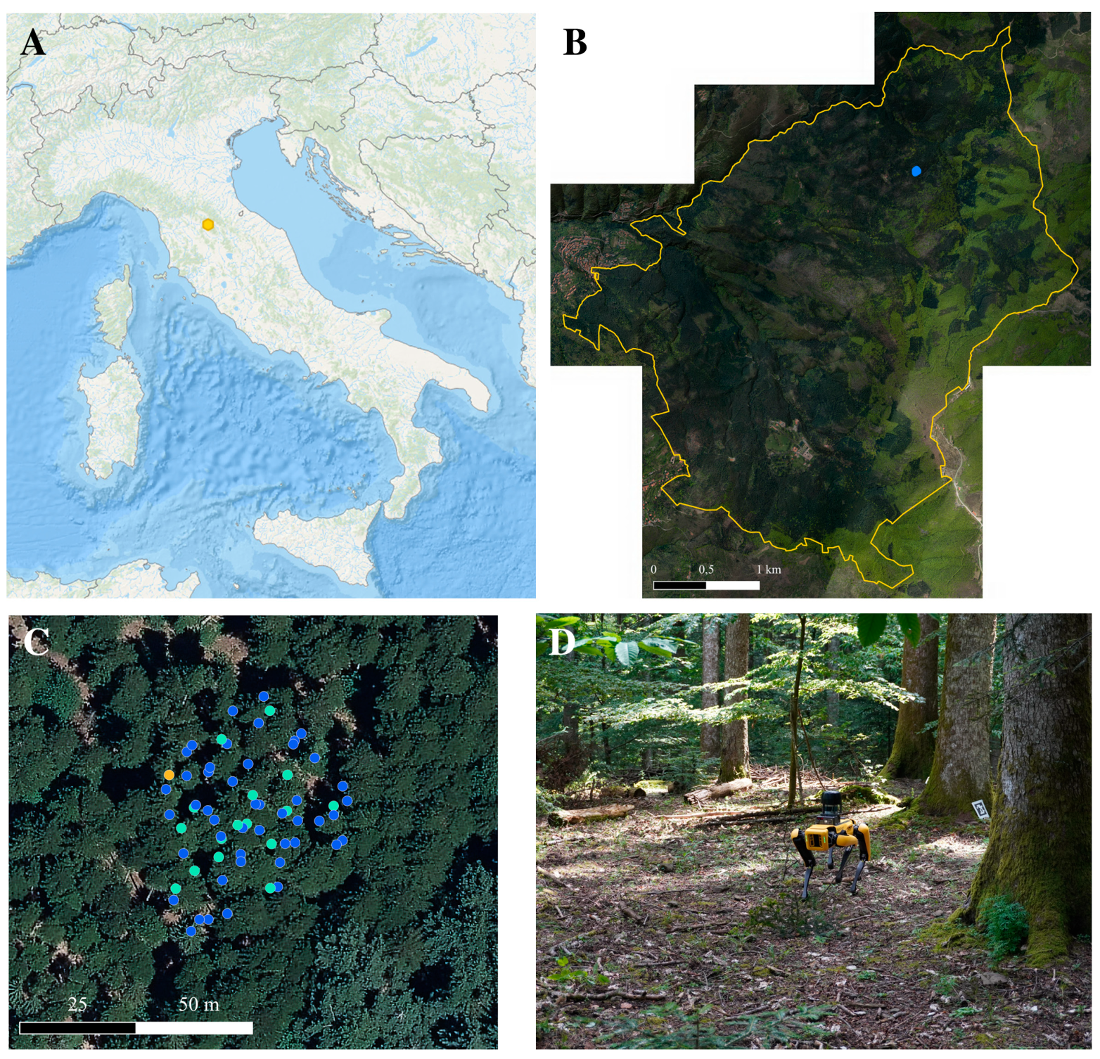
2.1. Test Site
The test site is located in the Vallombrosa Biogenetic National Nature Reserve in central Italy. The reserve extends for 1273 ha, with an altitude between 470 and 1447 m a.s.l. [
8,
21]. The analysis was conducted in a flat test area of 500 m
2 characterized by the presence of silver fir (
Abies alba Mill.), in the dominant layer, and European beech (
Fagus sylvatica L.), with sporadic presence of chestnut (
Castanea sativa L.), belonging to the European Forest Type no. 7.3—Apennine–Corsican mountainous beech forests [
22] (
Figure 1).
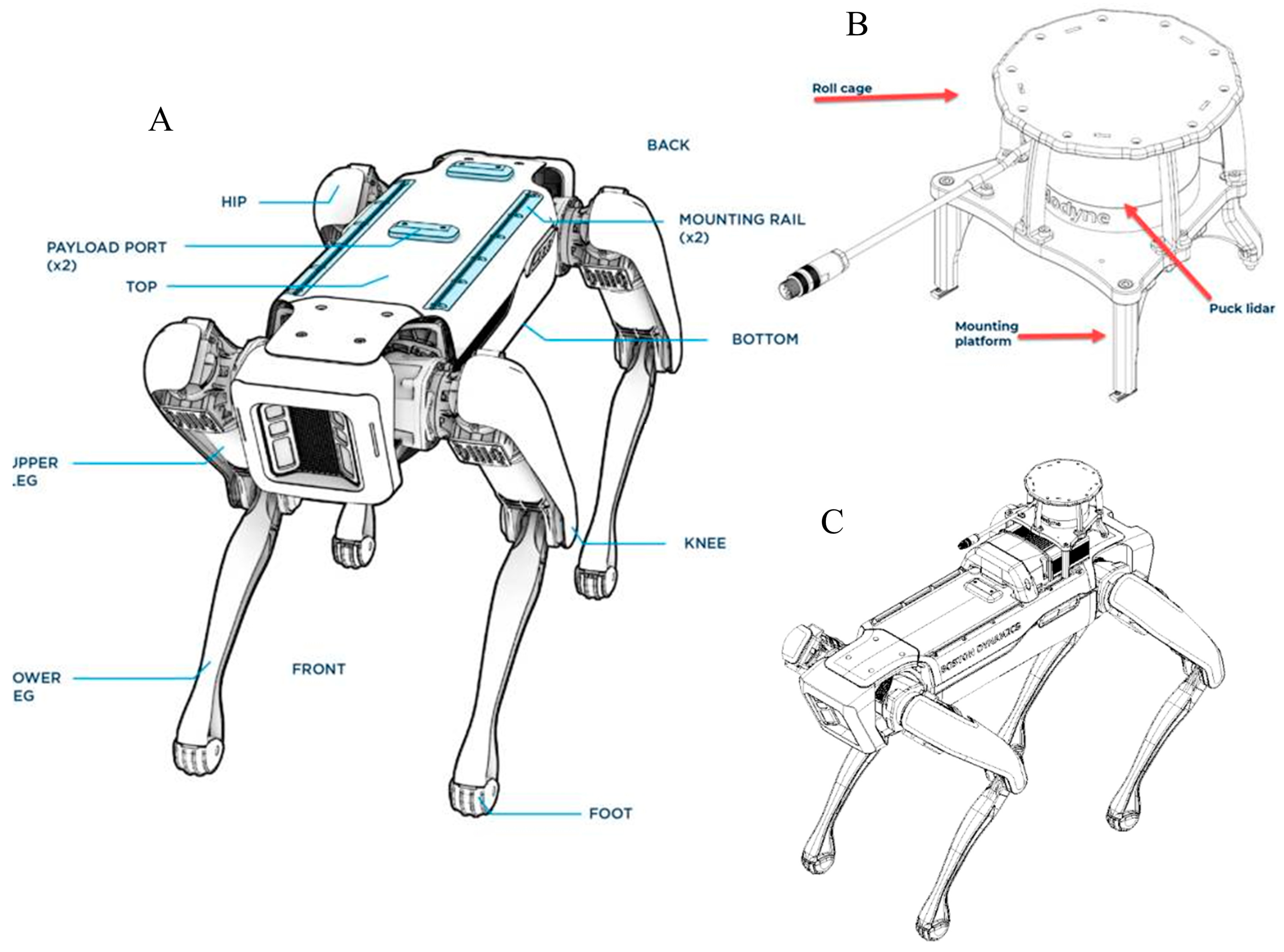
2.2. Overview of SPOT Capabilities and Functioning
The SPOT legged robot [
15], developed by Boston Dynamics, was used as a platform for teleoperated data collection. The robot, inspired by the physiognomy of the dog, is 1.10 m long and 0.50 m wide. It has an adjustable walking height from 0.52 to 0.70 m and a sitting height of 0.19 m for a total battery net weight of 32.7 kg. This robot can move at three different speeds up to 1.6 m s
−1, carrying up to 14 kg with two payload ports. SPOT’s main parts include the body, which houses computers and cameras, and the four legs, each composed of a hinged knee that connects the upper and lower sections of the leg and a ball joint at the hip where the upper leg connects to the body, for a total of 12 degrees of freedom (
Figure 2). The hip joints can perform an external/internal rotation of ±45° and a flexion/extension of ±91° with a deviation of 50° from the vertical, on the X and Y axis, respectively, while the knee joints have a flexion/extension range from 14° to 160°. Motors, cameras, sensors and payloads are powered by a single battery with a capacity of 564 Wh and a maximum voltage of 58.5 V, which requires a charging power of 400 W at a maximum current of 7 A. The battery autonomy in a typical runtime is around 90 min and up to 180 min in standby mode. SPOT can work in temperatures ranging from 0 °C to 40 °C. Charging time strongly depends on the ambient temperature and the type of charger: it varies between 50 min (Spot Dock charger at 25 °C) and 180 min (SPOT Dock charger at 35 °C). The expected battery life is around 500 cycles at 80% capacity. The weight of the battery varies between 4.2 kg (Explorer model) and 5.2 kg (Enterprise model).
SPOT is equipped with default with five optical cameras that allow a 360° field of view (FOV). Camera functions include: black-and-white and color fisheye, range (depth), and infrared. Five stereo pairs of depth cameras are used for depth perception and obstacle avoidance up to a distance of 2 m, with an FOV of ~90° in each direction, with four blind spots near the hip joints where FOV does not overlap. Obstacle avoidance is automatic and fully managed by SPOT software. The user can disable the obstacle avoidance function or modulate the minimum distance at which obstacles are detected to suit a wide range of situations and terrainn even in rough and obstacle-rich environments.
Nominally, the robot can walk in steep terrain, up to ±30°, in a temperature range of −20/+45 °C with illumination of at least 2 lux, making it particularly suitable for forestry applications. The maximum step height is 30 cm on flat terrain and 22 cm on stairs.
The SPOT enhanced autonomy payload (EAP), consisting of a SPOT CORE I/O GXP and a Velodyne VLP-16 LiDAR sensor, is placed in the front payload port to improve depth perception and detection capabilities up to ~120 m, recording the point cloud generated when working in Autowalk mode. The VLP-16 has a range of 100 m, and the sensor’s low power consumption (~8W), lightweight (0.83 kg), compact footprint (~Ø103 mm × 72 mm) and dual return capability make it ideal for UGVs and other mobile applications. Velodyne’s LiDAR Puck supports 16 channels, ~300,000 points/sec, a 360° horizontal field of view, and a 30° vertical field of view, with ±15° up and down shooting pulses at 903 nm wavelength. The Velodyne LiDAR Puck has no visible rotating parts, making it highly resistant in harsh environments. SPOT CORE I/O provides additional computing capability, with 48 tensor cores, NVIDIA Volta GPU for intensive tasks, and hosts the software required for the Velodyne LiDAR service to connect with the SPOT robot. SPOT GXP is a part of SPOT CORE and provides network and data interfaces and regulated power in an integrated package, greatly enhancing the computing and communications capabilities of the SPOT platform.
The fundamental aspects of SPOT operations, including walking, posing and safety, can be performed from a simple tablet or smartphone using the SPOT Boston Dynamics application. The robot is easy to use and autonomous in everything related to stability and obstacle avoidance. It features stand and walking modes and can be maneuvered using the joysticks on the SPOT tablet controller or touch-to-go mode on the controller screen. It also features an Autowalk mode that allows to record and replay autonomous behaviors. Autowalk consists of two parts:
recording missions: drive SPOT along a path and create actions (usually data acquisition) for the robot to carry out and perform along the way;
replaying a mission: SPOT will perform recorded movements and actions while adapting to small changes in the environment.
In the Autowalk mode, SPOT automatically places navigation waypoints along its path during mission recording and walks from waypoint to waypoint during mission replay. The basic SPOT platform tracks visual features within 2 m of the robot with stereo cameras. If SPOT is equipped with a LiDAR, it can track features within that sensor’s range, typically beyond 50 m. The additional detection range of LiDAR allows SPOT to travel away from features and through more dynamic environments. During mission replay, SPOT calculates its position by comparing the characteristics of current sensor data to those of data snapshots taken at each waypoint during mission recording. SPOT automatically compensates for deviations in its path and small changes in the environment, but large discrepancies may require operator intervention. Each mission must begin with a Fiducial, a specially designed image similar to QR codes that SPOT uses to match its internal map to the world around it. Fiducials are also used in locations with information gaps along the mission path to determine the location of SPOT.
2.3. Reference Measurements
All trees with a diameter at breast height (DBH) greater than 2.5 cm within the field test area were measured with a traditional caliper and their positions were measured using a Topcon GPT3000M topographic total station in combination with global navigation satellite systems (GNSSs) Topcon HiPer SR three-frequency receiver, observing the pseudo-range of GPS, GLONASS, and GALILEO satellites. The GNSS receiver was used to measure the location and orientation points of the total station used in post-processing to obtain the geographic coordinates. All data were collected from a total station positioned in the center of the test area. The polar coordinates of the trees at a height of 1.3 m were measured by length offset of the spatial polar method, which allows obtainment of Cartesian coordinates (x, y). Such coordinates were converted into geographic coordinates (WGS84UTM32N) using the two points measured with GNSS receiver in postprocessing. The resulting tree positions achieved sub-centimeter accuracy.
2.4. SPOT Data Acquisition
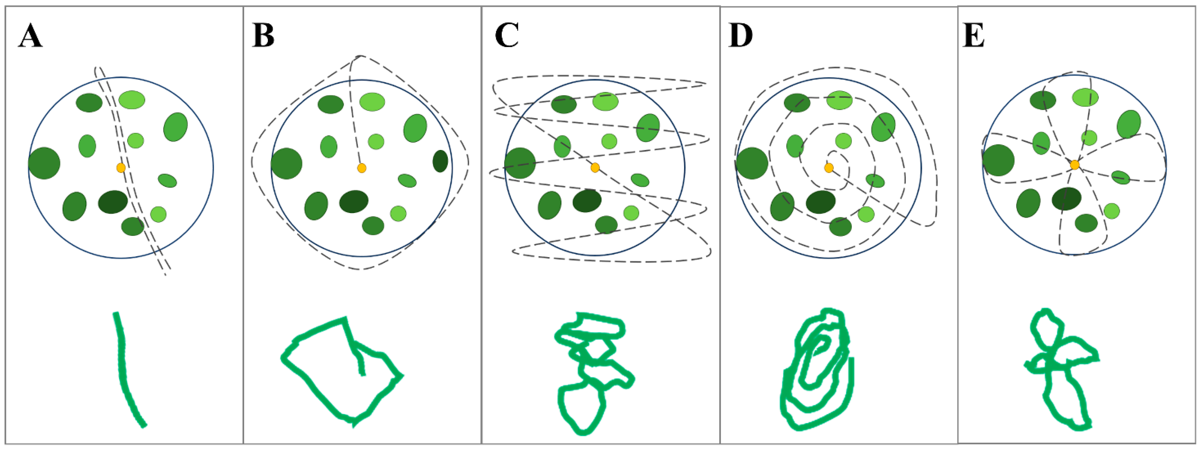
We tested a total of seven acquisition protocols to evaluate the performance of SPOT together with the EAP Velodyne LiDAR in tree detection and mapping and to assess the accuracy of DBH measurements. In each scan path, SPOT was teleoperated with a Wi-Fi connection with the remote controller, but SPOT used its ability to autonomously avoid the obstacles.
First, we simply guided SPOT to run a transect across the plot (A in
Figure 3) using a one-way at slow speed (OW slow) and then with two back-and-forth ways with both slow and medium speeds (TW slow and TW med, respectively). Second, we teleguided SPOT through more complex paths at medium speed with diamond, zig-zag, spiral and, finally, with a four-petal protocol (
Figure 3).
Each scan started and ended (i.e., the initialization of each Autowalk mode) approximately at the center of the test area, where a fiducial was placed to ensure a closed loop, as required when the SLAM (simultaneous localization and mapping) algorithm is used [
11,
23]. The time required to perform each scan and the length of the path were recorded.
2.5. Tree Detection and DBH Estimation
The final tree position and DBH assessment processing workflows were the same for all point clouds obtained from SPOT paths. Velodyne point cloud data were processed via R-CRAN using the lid-R, TreeLS, and rlas packages.
To segment the point clouds obtained from the different protocols into a single tree, a common procedure was followed using terrestrial or mobile laser scanner. First, the point clouds were classified into ground and non-ground using the cloth simulation filter (CFS) algorithm by Zhang et al. [
24] and implemented in the lid-r package. Second, the point cloud was normalized using the classified ground terrain.
The normalized point clouds were then processed using the treeMap. StemPoint functions implemented in TreeLS into single tree. The Hough transform (HT) method was used in both functions. The HT circle search algorithm applies a constrained circle search on discretized point cloud layers. Tree-wise, the circular search is recursive, where the search for the circle parameters of a stem section is constrained to the feature space of the underlying stem section. Initial estimates of the stem feature space are performed on a baseline stem segment, i.e., a low height interval where a tree stem is expected to be clearly visible in the point cloud: the algorithm is described in detail by de Conto et al. [
25]. The two functions allow extraction of the positions of each tree. Then, for each segmented tree, forest inventory data were automatically extracted using tlsInventory function implemented in TreeLS which allows obtainment of the estimates of DBH and H for a normalized point cloud with assigned stem points. At the end of the procedure for each tree, we obtained the Cartesian coordinates position in a Cartesian coordinate system. The results were then rototranslated in geographic coordinate system according to the benchmark field reference using three trees recognized in the cloud manually. The results were finally clipped within the test area. Indeed, since some survey protocols required SPOT to walk in the borders of the test area, and since the sensor has detection capabilities up to 120 m, other trees had also been detected.
2.6. Data Evaluation
Tree positions and DBHs were calculated from the point clouds generated by each protocol presented in
Figure 3. The estimated DBH and position of the trees were compared with field-measured reference data, considering only trees with DBH greater than 20 cm. First, manual co-registration was performed in QGIS software by identifying pairs of corresponding survey trees. Specifically, the raw data had relative metric coordinates (surveys started with coordinates 0, 0), which were converted to absolute coordinates of the center of the study area. Then, each protocol was appropriately georeferenced by translating the surveyed trees in concordance with the reference trees. Finally, for each identified tree, the best match was manually identified [
26] based on location, DBH and spatial pattern of neighboring trees.
2.7. Position Error
The estimated position error of each tree was calculated both as bias on the X and Y coordinates and as the Euclidean distance between the estimated position and the reference position measured by the total station. The bias was calculated as the average difference between the estimated coordinates and those measured with the Topcon station, both for X and Y. Furthermore, the azimuth in decimal degrees, ranging between 0 and 360 clockwise from north, was calculated from each pair of estimated position and reference one. The final position error was calculated by averaging the individual tree distance within each protocol.
2.8. DBH Error
We calculated the estimation errors in DBH when all pairs of trees were identified. Errors were calculated in terms of bias, root-mean-squared error (RMSE) and percentage RMSE (RMSE%) with respect to the average reference DBH:
where
and
are the measured and estimated DBH, respectively, and
n is the number of trees measured in each protocol.
3. Results
3.1. Total Station Reference Measurements
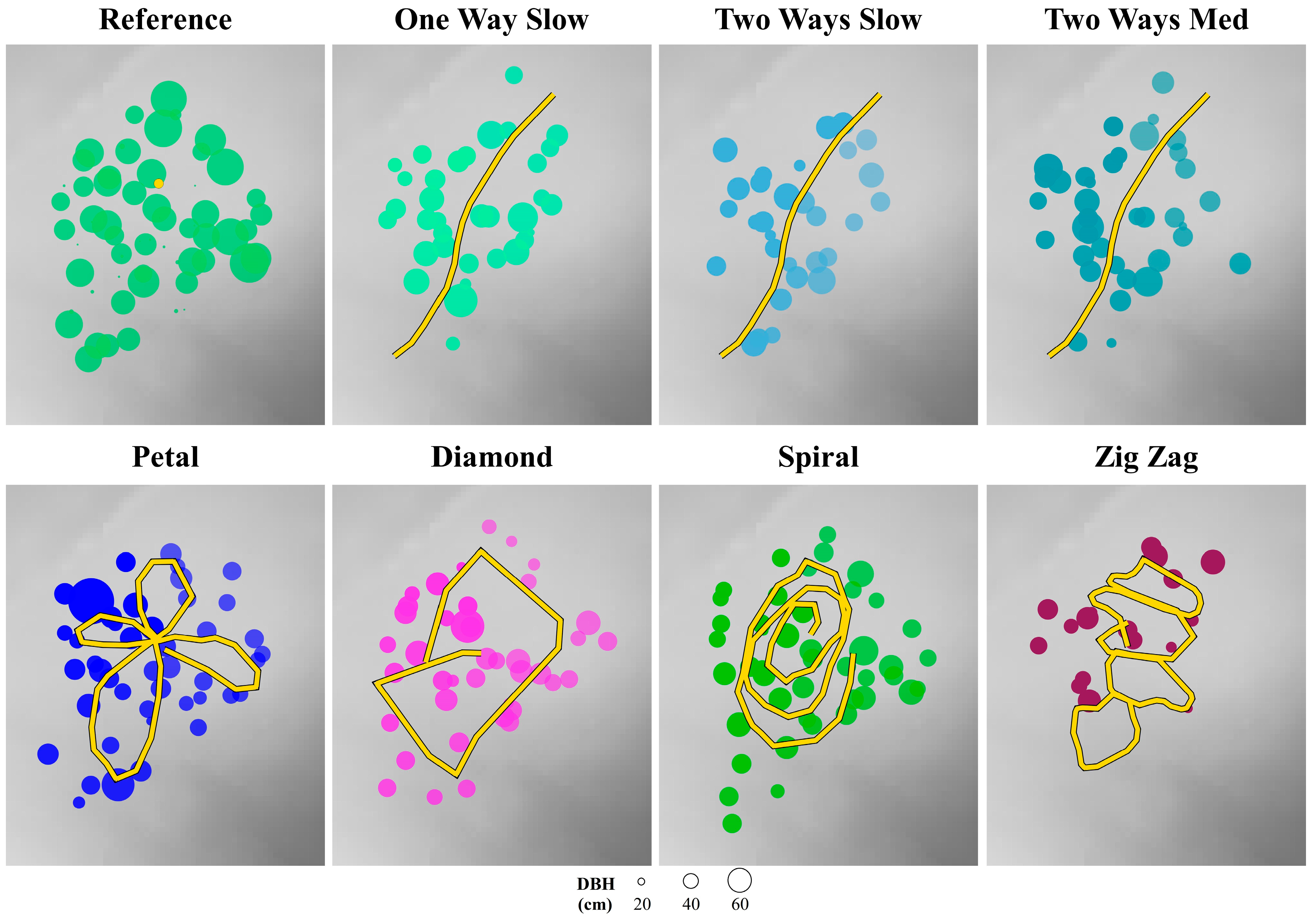
A total of 67 trees were measured and calipered, of which 45 had a DBH ≥ 20 cm (
Figure 4). The mean DBH measured in the field was 58.3 cm.
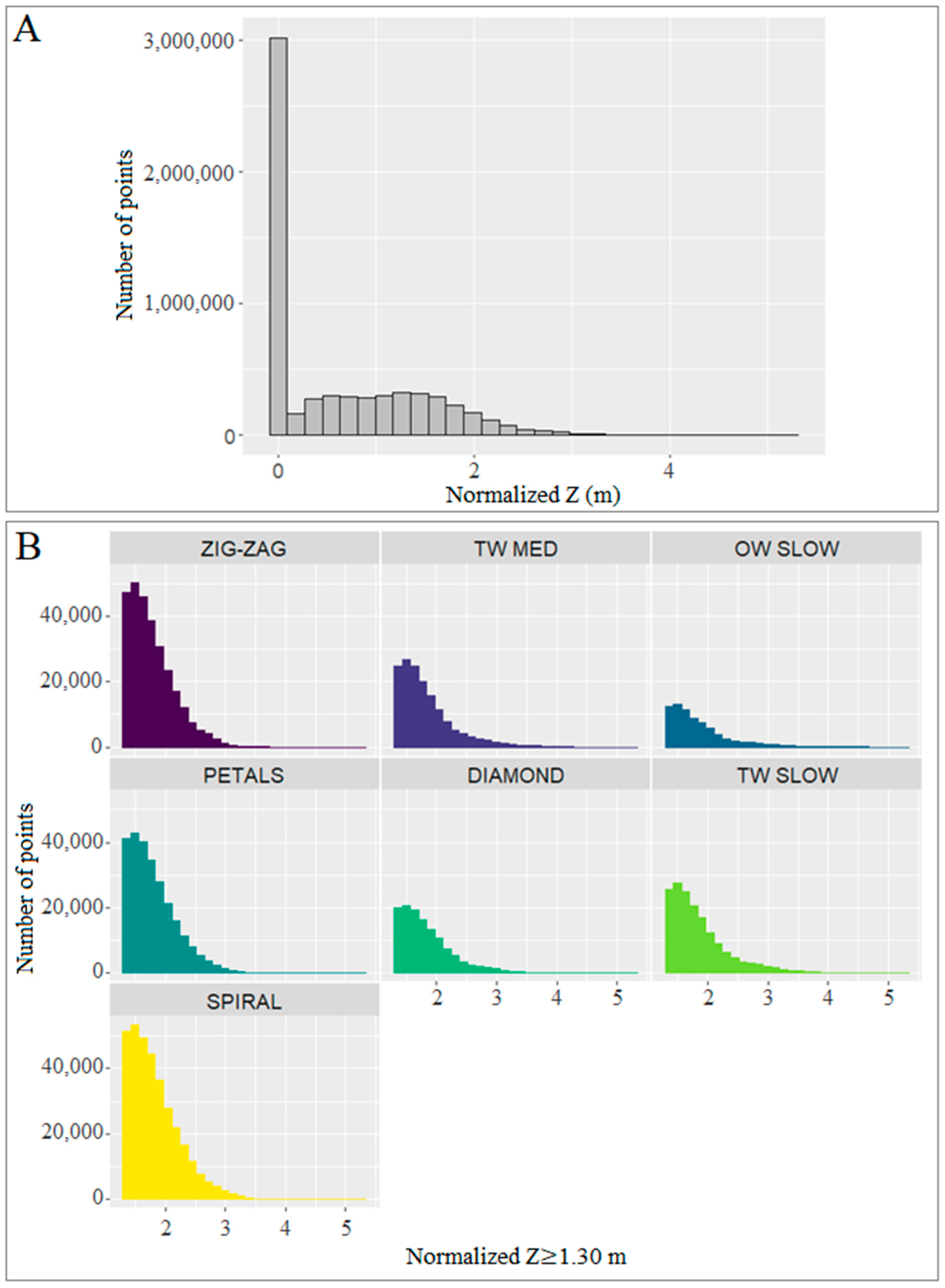
A point cloud was obtained from each one of the field-tested protocols. The acquisition path that allows obtaining a denser point cloud in terms of point/m
2 was the “zig-zag,” followed by “spiral” and “petals” (
Table 1). These paths allow obtainment of point clouds with a point density greater than 110 point/m
2, while the “diamond,” “TW_slow, “OW_Med” paths allow obtainment of comparable densities between 74.27 and 76.48 point/m
2 (
Table 1). The path OW_slow obtained the lowest point/density of 41.38 point/m
2.
By analyzing the distribution of points along the Z for the normalized point clouds, the majority of the points proved to be recorded in the ground (normalized Z = 0), and the majority of the remaining points were located in the Z range between 0.1 and 2 m, while few points reached a normalized Z of 3–5 m (
Figure 5).
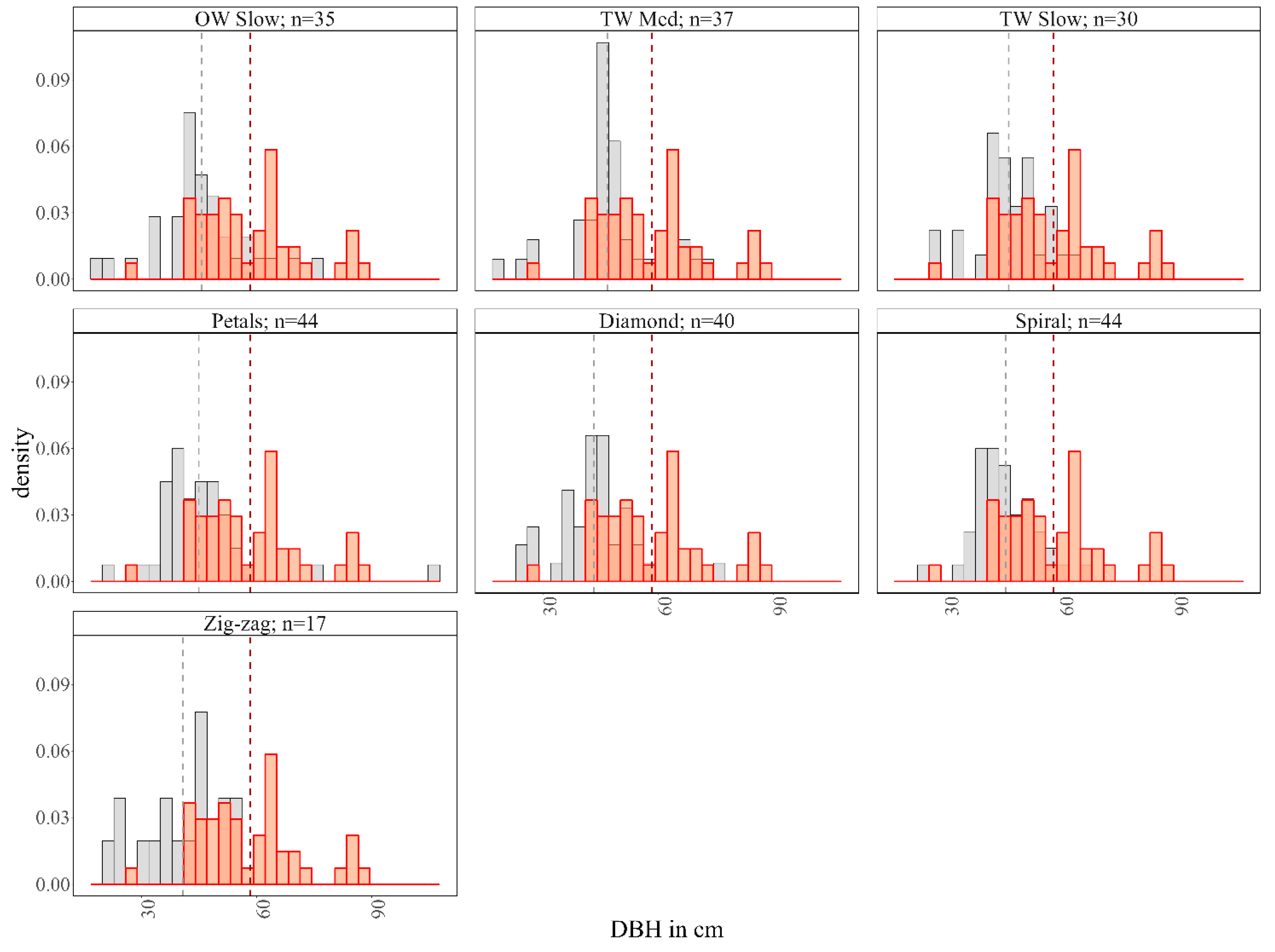
3.2. Tree DBH Errors
Due to the noise in the point cloud, only a few small trees were identified. For this reason, we focused our comparative analysis on trees with DBH ≥ 20 cm. In the different protocols, the number of trees detected varied between 17 (for the zig-zag protocol) and 44 (for the petals and spiral protocols) against the 45 measured in the benchmark. The mean DBH varied from 40.8 cm (zig-zag protocol) to 46.6 cm (TW med and TW slow protocols) (
Table 2) against the true value of 58.3 cm.
Figure 6 shows the DBH > 20 cm distribution from each protocol against the reference DBH distribution. The RMSE% ranged from a minimum of 39.6 for the TW slow protocol to a maximum of 56.9 for the zig-zag protocol.
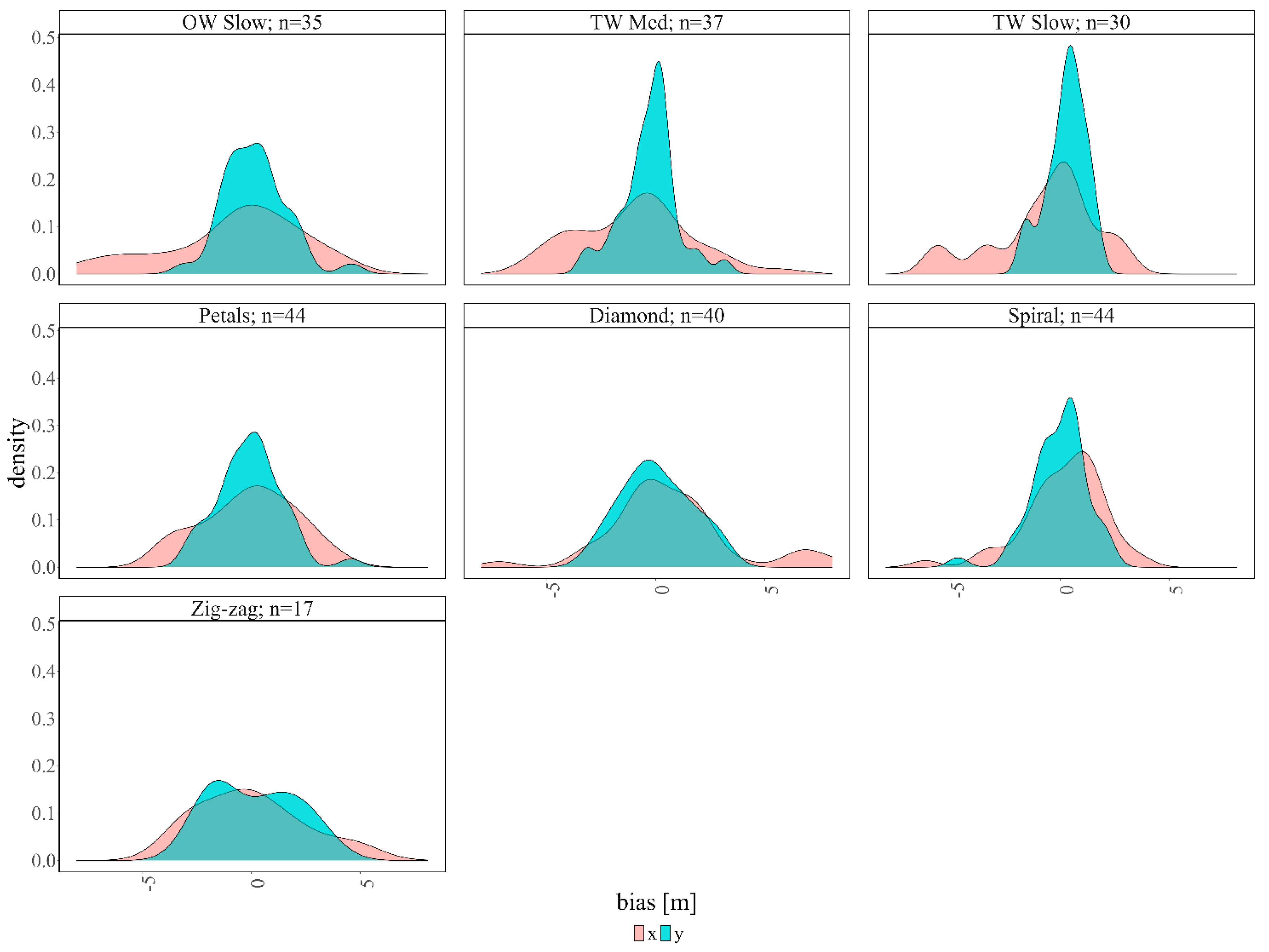
3.3. Tree Positioning Errors
The average distance between observed tree position and that estimated by SPOT acquisitions ranged between 1.9 m (spiral protocol) and 2.9 m (OW slow protocol) (
Table 3), with a minimum single distance of 0.09 m and a maximum of 8.13. The zig-zag protocol achieved the minimum bias on the X coordinate (0 m), while the petals and diamond protocols achieved the minimum bias on the Y one (0 m). The maximum bias on the X coordinate was −0.8 m (protocol OW slow), while it was ±0.3 on the Y one (protocols TW slow and TW med). The minimum and maximum absolute difference were 0.002 and 8.1 m and 0.006 and 4.7 m in the X and Y coordinates, respectively (
Figure 7).
4. Discussion
With this contribution, we have presented for the first time in the scientific literature the potential of the SPOT legged robot to support forest inventory and mensuration by individual tree detection, mapping and DBH measurements using the LiDAR EAP systems on board.
SPOT was driven via teleoperation by an operator with no prior specific experience. From this point of view, SPOT was easy to drive and its autonomous ability to avoid obstacles worked well in the field, although the test area was quite flat and almost, but not completely, free of obstacles such as stones, small plants and deadwood. This is especially true when SPOT was used at slow or medium speed. For this reason, in complex forest terrain, we recommend avoiding use at higher speed.
The point clouds recorded by the Velodyne LiDAR of the EAP SPOT system in the different acquisitions in our test area ranged between 41 and 152 pulses/m
2, but the vast majority of the returns were for relative heights from the ground not higher than 3 meters. Most of the pulses returned from the ground (
Figure 5).
Results in identifying large trees were strongly influenced by the differences in cloud density. However, it was impossible to identify small trees (DBH < 20 cm) regardless of cloud characteristics.
When SPOT was operated at low speed, the results were slightly better, but without strong differences from those obtained with medium speed, while the results in DBH measurements when more complex paths were run resulted in denser point clouds. The results of DBH measurements showed RMSE% of 40% for TW at medium and low speed and below 50% for OW, spiral, and diamond protocols. With the petals and spiral patterns, it was possible to correctly identify 97% of the large trees. With the zig-zag pattern, the resulting point cloud was dense but the result in the identification of the trees was poor, most likely because the frequent changes in the walking direction of the robot negatively impacted the SLAM procedure and therefore the tree identification.
Regarding the positioning of the trees, the test area elongated in the north–south direction resulted in less bias in identifying trees according to the y coordinate. However, although the bias in X and Y coordinates was quite normally distributed (
Figure 7), the resulting error in tree positioning was consistent: only with the spiral pattern was it possible to have an average positioning error lower than 2 m. Once again, the density of the point cloud significantly influenced the results.
5. Conclusions
Forest tree monitoring and assessment are rapidly evolving as new information needs arise and new techniques and tools become available. However, the exploitation of the latter, as well as their implementation within operative management processes, should be evidence-based [
28]. From this perspective, based on this first experience with SPOT and from the comparison with a traditional forest survey, some pros and cons clearly emerged so far.
The pros are that the SPOT robot is able to move in the forest terrain, autonomously avoiding obstacles, at least in the conditions we experienced in this first test and if maneuvered at slow speed. It is therefore plausible that in the future systems could be developed for a more automatic acquisition of point clouds with SPOT to avoid the need for teleoperation. The battery use of SPOT is also good as it easily reaches its maximum nominal potential: this is an important aspect because SPOT is quite heavy and if it is not able to walk, its transportation in the field is not easy.
The cons are mainly due to the limited capacity of its EAP LiDAR system. Even though the hardware (the Velodyne LiDAR) has excellent potential, a formal SLAM procedure is not yet implemented in the SPOT system and the resulting point clouds are noisy and difficult to interpret (trees smaller than 20 cm are almost not detected). SPOT’s ability to move its torso to direct the laser pulses in different directions is good, even though the resulting cloud had a maximum height above the ground of about 3 m. In this way, it is possible to measure the DBH of the trees, but not their height. Of course, the SPOT LiDAR cloud can be combined with the pulses from ALS to create a more complete assessment of 3D forest structure.
It is important to note that the accuracy of the results (especially in DBH measurements) was highly variable in the different protocols tested, mainly due to the different densities of the resulting point cloud.
In the near future, we will continue to explore SPOT capabilities for forest inventory support with a different TLS system connected to payload docks, capable of implementing a better SLAM procedure. Furthermore, the SPOT’s capabilities could be further explored for monitoring and analysis of forest tree plantations, both in stands for industrial timber production (e.g., hybrid poplar plantations) and in short-rotation forestry. In fact, these plantations, which play a significant role in wood production [
29], are typically located in flat areas and with homogeneous conditions, particularly suitable for SPOT. Future research could also explore the feasibility of assessing forest-floor biodiversity attributes, such as fallen trees, coarse woody debris, and trunk- and root-related microhabitats [
30,
31], which can usually require significant time and manual effort during field inventories [
32]. In this context, the wide range of movements of SPOT could overcome the problems related to static terrestrial laser scanning in detection of microhabitats [
33,
34].
From these first results, the future use of legged robots seems to be promising to support forest inventory and mensuration, especially if systems for carrying out missions in a totally autonomous manner become possible, as is already possible with UAVs.
Author Contributions
Conceptualization, G.C.; formal analysis, F.G., G.D. and E.V.; investigation, G.D., E.V., S.F. and C.B.; data curation, F.G., G.D. and E.V.; writing—original draft preparation, F.G., G.D., E.V., S.F. and C.B.; writing—review and editing, G.C., P.C. and D.T. All authors have read and agreed to the published version of the manuscript.
Funding
The research received support to buy the Boston Dynamics SPOT legged robot from the University of Florence within the call “Bando di Ateneo per l’acquisizione di strumenti finalizzati alla ricerca nell’ambito delle tematiche del PNR 2021-2027—Anno 2022”.
Data Availability Statement
The data that support the findings of this study are available from the authors upon reasonable request.
Conflicts of Interest
The authors declare no conflict of interest.
References
- Hamedianfar, A.; Mohamedou, C.; Kangas, A.; Vauhkonen, J. Deep learning for forest inventory and planning: A critical review on the remote sensing approaches so far and prospects for further applications. Forestry 2022, 95, 451–465. [Google Scholar] [CrossRef]
- Bechar, A.; Vigneault, C. Agricultural robots for field operations. Part 2: Operations and systems. Biosyst. Eng. 2017, 153, 110–128. [Google Scholar] [CrossRef]
- Sun, H.; Yan, H.; Hassanalian, M.; Zhang, J.; Abdelkefi, A. UAV Platforms for Data Acquisition and Intervention Practices in Forestry: Towards More Intelligent Applications. Aerospace 2023, 10, 317. [Google Scholar] [CrossRef]
- Visser, R.; Obi, O.F. Automation and robotics in forest harvesting operations: Identifying near-term opportunities. Croat. J. For. Eng. J. Theory Appl. For. Eng. 2021, 42, 13–24. [Google Scholar] [CrossRef]
- Tang, L.; Shao, G. Drone remote sensing for forestry research and practices. J. For. Res. 2015, 26, 791–797. [Google Scholar] [CrossRef]
- Oliveira, L.F.P.; Moreira, A.P.; Silva, M.F. Advances in Forest Robotics: A State-of-the-Art Survey. Robotics 2021, 10, 53. [Google Scholar] [CrossRef]
- Fardusi, M.J.; Chianucci, F.; Barbati, A. Concept to Practice of Geospatial-Information Tools to Assist Forest Management and Planning under Precision Forestry Framework: A review. Ann. Silvic. Res. 2017, 41, 3–14. [Google Scholar] [CrossRef]
- Giannetti, F.; Puletti, N.; Puliti, S.; Travaglini, D.; Chirici, G. Assessment of UAV photogrammetric DTM-independent variables for modelling and mapping forest structural indices in mixed temperate forests. Ecol. Indic. 2020, 117, 106513. [Google Scholar] [CrossRef]
- Puliti, S.; Granhus, A. Drone data for decision making in regeneration forests: From raw data to actionable insights. J. Unmanned Veh. Syst. 2021, 9, 45–58. [Google Scholar] [CrossRef]
- Fankhauser, P.; Hutter, M. ANYmal: A Unique Quadruped robot conquering harsh environments. Res. Features 2018, 126, 54–57. [Google Scholar]
- Idrissi, M.; Hussain, A.; Barua, B.; Osman, A.; Abozariba, R.; Aneiba, A.; Asyhari, T. Evaluating the Forest Ecosystem through a Semi-Autonomous Quadruped Robot and a Hexacopter UAV. Sensors 2022, 22, 5497. [Google Scholar] [CrossRef] [PubMed]
- Chen, G.; Hong, L. Research on Environment Perception System of Quadruped Robots Based on LiDAR and Vision. Drones 2023, 7, 329. [Google Scholar] [CrossRef]
- Koval, A.; Kanellakis, C.; Nikolakopoulos, G. Evaluation of Lidar-based 3D SLAM algorithms in SubT environment. IFAC-PapersOnLine 2022, 55, 126–131. [Google Scholar] [CrossRef]
- Crespo, C.; Rodríguez, F. Integration of robotics in underground mining construction works. In Proceedings of the Expanding Underground-Knowledge and Passion to Make a Positive Impact on the World-Proceedings of the ITA-AITES World Tunnel Congress, WTC 2023, Athens, Greece, 12–18 May 2023; CRC Press: Boca Raton, FL, USA, 2023; pp. 2414–2421. [Google Scholar] [CrossRef]
- Koval, A.; Karlsson, S.; Nikolakopoulos, G. Experimental evaluation of autonomous map-based spot navigation in confined environments. Biomim. Intell. Robot. 2022, 2, 100035. [Google Scholar] [CrossRef]
- Afsari, K.; Halder, S.; Ensafi, M.; DeVito, S.; Serdakowski, J. Fundamentals and Prospects of Four-Legged Robot Application in Construction Progress Monitoring. In Proceedings of the 57th Annual Associated Schools of Construction International Conference, Chico, CA, USA, 5–9 April 2021; pp. 263–274. [Google Scholar] [CrossRef]
- Wetzel, E.M.; Liu, J.; Leathem, T.; Sattineni, A. The Use of Boston Dynamics SPOT in Support of LiDAR Scanning on Active Construction Sites. In Proceedings of the 39th ISARC, Bogotá, Colombia, 13–15 July 2022. [Google Scholar] [CrossRef]
- Wetzel, E.M.; Umer, M.; Richardson, W.; Patton, J. A Step Towards Automated Tool Tracking on Construction Sites: Boston Dynamics SPOT and RFID. EPiC Ser. Built Environ. 2022, 3, 478–488. [Google Scholar] [CrossRef]
- Yunus, A.; Doore, S.A. Responsible use of agile robots in public spaces. In Proceedings of the IEEE International Symposium on Ethics in Engineering, Science and Technology, Waterloo, ON, Canada, 28–31 October 2021. [Google Scholar] [CrossRef]
- Due, B.L. A Walk in the Park with Robodog: Navigating Around Pedestrians Using a Spot Robot as a “Guide Dog”. Space Cult. 2023. [Google Scholar] [CrossRef]
- Ciancio, O. Riserva Naturale Statale Biogenetica di Vallombrosa. Piano di Gestione e Silvomuseo 2006–2025; Corpo Forestale dello Stato; Ufficio Territoriale per la Biodiversità di Vallombrosa; Tipografia Coppini: Firenze, Italy, 2009. [Google Scholar]
- Barbati, A.; Marchetti, M.; Chirici, G.; Corona, P. European forest types and forest europe SFM indicators: Tools for monitoring progress on forest biodiversity conservation. For. Ecol. Manag. 2014, 321, 145–157. [Google Scholar] [CrossRef]
- Tang, J.; Chen, Y.; Kukko, A.; Kaartinen, H.; Jaakkola, A.; Khoramshahi, E.; Hakala, T.; Hyyppä, J.; Holopainen, M.; Hyyppä, H. SLAM-aided stem mapping for forest inventory with small-footprint mobile LiDAR. Forests 2015, 6, 4588–4606. [Google Scholar] [CrossRef]
- Zhang, W.; Qi, J.; Wan, P.; Wang, H.; Xie, D.; Wang, X.; Yan, G. An easy-to-use airborne LiDAR data filtering method based on cloth simulation. Remote Sens. 2016, 8, 501. [Google Scholar] [CrossRef]
- De Conto, T.; Olofsson, K.; Görgens, E.B.; Rodriguez, L.C.E.; Almeida, G. Performance of stem denoising and stem modelling algorithms on single tree point clouds from terrestrial laser scanning. Comput. Electron. Agric. 2017, 143, 165–176. [Google Scholar] [CrossRef]
- Mokroš, M.; Mikita, T.; Singh, A.; Tomaštík, J.; Chudá, J.; Wężyk, P.; Kuželka, K.; Surový, P.; Klimánek, M.; Zięba-Kulawik, K.; et al. Novel low-cost mobile mapping systems for forest inventories as terrestrial laser scanning alternatives. Int. J. Appl. Earth Obs. Geoinf. 2021, 104, 102512. [Google Scholar] [CrossRef]
- Giannetti, F.; Puletti, N.; Quatrini, V.; Travaglini, D.; Bottalico, F.; Corona, P.; Chirici, G. Integrating terrestrial and airborne laser scanning for the assessment of single-tree attributes in Mediterranean forest stands. Eur. J. Remote Sens. 2018, 51, 795–807. [Google Scholar] [CrossRef]
- Corona, P. Communicating facts, findings and thinking to support evidence-based strategies and decisions. Ann. Silvic. Res. 2018, 42, 1–2. [Google Scholar]
- D’Amico, G.; Francini, S.; Giannetti, F.; Vangi, E.; Travaglini, D.; Chianucci, F.; Mattioli, W.; Grotti, M.; Puletti, N.; Corona, P.; et al. A deep learning approach for automatic mapping of poplar plantations using Sentinel-2 imagery. GIScience Remote Sens. 2021, 58, 1352–1368. [Google Scholar] [CrossRef]
- Bradley, H.S.; Craig, M.D.; Cross, A.T.; Tomlinson, S.; Bamford, M.J.; Bateman, P.W. Revealing microhabitat requirements of an endangered specialist lizard with LiDAR. Sci. Rep. 2022, 12, 5193. [Google Scholar] [CrossRef] [PubMed]
- Larrieu, L.; Paillet, Y.; Winter, S.; Bütler, R.; Kraus, D.; Krumm, F.; Lachat, T.; Michel, A.K.; Regnery, B.; Vandekerkhove, K. Tree related microhabitats in temperate and Mediterranean European forests: A hierarchical typology for inventory standardization. Ecol. Indic. 2018, 84, 194–207. [Google Scholar] [CrossRef]
- Rehush, N.; Abegg, M.; Waser, L.T.; Brändli, U.B. Identifying tree-related microhabitats in TLS point clouds using machine learning. Remote Sens. 2018, 10, 1735. [Google Scholar] [CrossRef]
- Siitonen, J.; Pasanen, H.; Ylänne, M.; Saaristo, L. Comparison of four alternative survey methods in assessing dead wood at the stand level. Scand. J. For. Res. 2023, 38, 244–253. [Google Scholar] [CrossRef]
- Frey, J.; Asbeck, T.; Bauhus, J. Predicting Tree-Related Microhabitats by Multisensor Close-Range Remote Sensing Structural Parameters for the Selection of Retention Elements. Remote Sens. 2020, 12, 867. [Google Scholar] [CrossRef]
| Disclaimer/Publisher’s Note: The statements, opinions and data contained in all publications are solely those of the individual author(s) and contributor(s) and not of MDPI and/or the editor(s). MDPI and/or the editor(s) disclaim responsibility for any injury to people or property resulting from any ideas, methods, instructions or products referred to in the content. |
© 2023 by the authors. Licensee MDPI, Basel, Switzerland. This article is an open access article distributed under the terms and conditions of the Creative Commons Attribution (CC BY) license (https://creativecommons.org/licenses/by/4.0/).


 ,
, 


