Land Cover Classification of Remote Sensing Images Based on Hierarchical Convolutional Recurrent Neural Network

Abstract

Convolutional neural networks (CNNs) and recurrent neural networks (RNNs) have gained improved results in remote sensing image data classification. Multispectral image classification can benefit from the rich spectral information extracted by these models for land cover classification. This paper proposes a classification model called a hierarchical convolutional recurrent neural network (HCRNN) to combine the CNN and RNN modules for pixel-level classification of multispectral remote sensing images. In the HCRNN model, the original 13-band information from Sentinel-2 is transformed into a 1D multispectral sequence using a fully connected layer. It is then reshaped into a 3D multispectral feature matrix. The 2D-CNN features are extracted and used as inputs to the corresponding hierarchical RNN. The feature information at each level is adapted to the same convolution size. This network structure fully leverages the advantages of CNNs and RNNs to extract temporal and spatial features from the spectral data, leading to high-precision pixel-level multispectral remote sensing image classification. The experimental results demonstrate that the overall accuracy of the HCRNN model on the Sentinel-2 dataset reaches 97.62%, which improves the performance by 1.78% compared to the RNN model. Furthermore, this study focused on the changes in forest cover in the study area of Laibin City, Guangxi Zhuang Autonomous Region, which was 7997.1016 km², 8990.4149 km², and 8103.0020 km² in 2017, 2019, and 2021, respectively, with an overall trend of a small increase in the area covered.

1. Introduction

Land is a fundamental element for human survival and serves as a crucial foundation for social and economic development. Land is closely related to the human living environment and crop production, and yet it is also closely related to most of the pressing challenges facing mankind [1,2,3]. The gradual development of remote sensing technology makes it play an increasingly important role in the fields of environmental monitoring, geological exploration, precision agriculture, and land cover mapping [4,5,6,7,8,9]. Among these applications, land cover classification, which is a vital component of remote sensing technology, has always been a prominent area of research and a challenging task in extracting valuable information from remote sensing images. How to recognize different features and classify them with high accuracy using remote sensing images, as well as the statistics of various types of feature information, is a key concern in the field.

In the past decades of research, scholars have studied and discussed various types of supervised classification models. These models include the maximum likelihood (ML) [10,11], support vector machine (SVM) [12], and random forest(RF) [13,14]. In this case, the maximum likelihood method is based on the assumption that the statistical distribution of each category conforms to a normal distribution, and classification is achieved by calculating the likelihood that an input pixel belongs to a particular category. Support vector machine (SVM) is a supervised classification model that has been widely used in various applications with great success. In the classification of multispectral images, support vector machine has been proved an effective method. The model separates the data by investigating the optimal classification decision hyperplane, making it possible to better divide the training samples in a high-dimensional feature space. Random forest is a supervised classification model based on multiple decision trees. The model obtains the final prediction by randomly sampling the input spectral pixel sequences generating multiple decision trees and then combining the outputs of these decision trees through a voting mechanism. However, with the wide application of various multispectral or high-resolution remote sensing satellite image products, the classification accuracy of the traditional methods needs to be improved. To get around this problem, a deep learning approach was used for land cover classification.

Deep learning methods have significantly enhanced the capabilities of land cover classification by excelling in feature learning and prediction. Compared to traditional methods, deep learning techniques are capable of extracting more complex structural features from the data and possess superior feature selection and data noise processing capabilities. Particularly in recent years, deep learning has developed more and more rapidly, and it has become the mainstream method for land cover classification [15,16,17]. Among these methods, the backpropagation (BP) neural network, a widely adopted artificial neural network, has demonstrated excellent performance in remote sensing classification. B. Ahmed et al. [18] used the spectral and texture features of high-resolution images of Beijing as inputs to a BP neural network and used a backpropagation neural network (BPNN) to find a set of weights that minimized the error, thus completing the training of the network and obtaining classification results. Semantic segmentation is the segmentation of an entire remote sensing image by pixel-level classification, where each pixel is assigned to a different category. This method can extract the classification result for each pixel in the image [19]. U-Net [20] is a classical network architecture for dealing with semantic segmentation problems, which was initially widely used in the field of biomedical images. In recent years, U-Net and its variants have also been gradually used for land cover classification tasks due to their ability to achieve better segmentation results with relatively less data and in a shorter time. Stoian A et al. [21] proposed FG-Unet, a network architecture specialized in processing sparsely annotated data and maintaining high-resolution image output, which was successfully used for land cover classification tasks in the Mediterranean region. Zhang P et al. [22] proposed a model called Asp-Unet that consists of contraction paths with high-level features and generates high-resolution outputs by creating expansion paths. The model used the pyramid pooling (Aspp) technique for multi-scale feature fusion at the bottom layer to generate discriminative features. Chen S et al. [23] enhanced the conventional U-Net semantic segmentation network by replacing the original U-Net convolution unit with a residual convolution module. This modification increased the network’s depth and improved its segmentation performance, especially for small target categories.

Convolutional neural networks (CNNs) and recurrent neural networks (RNNs) are widely used deep learning models in remote sensing data classification, and they have achieved good results in this field. Convolutional neural networks (CNNs) can learn and extract advanced spatial features efficiently due to their multi-layer feature extraction capability [24]. Ce Zhang et al. [25] came out with a new convolutional neural network (OCNN) specifically applied to land use, whose functional unit is object-based segmentation. In addition, Hu et al. [26] proposed a 1D-CNN network for hyperspectral data classification, whose structure contains an input layer, a convolutional layer, a max-pooling layer, and a fully connected layer. To improve classification accuracy, researchers have also developed variant CNN structures, including 2D-CNN and 3D-CNN. Although CNN can extract spectral information and semantic features from satellite images, 1D-CNN can only handle one-dimensional sequence data and cannot deal with time series features. Thus, these new CNN variants can better handle multidimensional data and improve classification accuracy. Lu Y et al. [27] presented a hybrid 2D and 3D CNN model, which firstly utilizes multiple 3D-CNN modules to extract spatiotemporal features and downscale the output feature sequence. Then, the downscaled features are used as inputs to the 2D-CNN module, and, finally, the fully connected layer is used to predict the class of the feature. Thus far, 2D-CNN cannot extract time-scale information, while 3D-CNN is computationally complex with a much larger number of parameters [28].

Recurrent neural networks (RNNs) have great applications in processing time series data in multispectral remote sensing images. R. Hang et al. [29] designed a backbone network consisting of two RNN layers. The first RNN layer efficiently reduces redundant information in adjacent spectral bands, simplifying the spectral feature information to be fed into the second RNN layer for feature complementation. With the advancement of RNNs, novel variants such as long short-term memory (LSTM) and gated recurrent unit (GRU) have been introduced to tackle the gradient vanishing problem and capture long-term dependencies. Feng Q et al. [30] designed a bi-directional LSTM model to obtain spatio-temporal sequence features in UAV images. This model stacks two LSTMs, inputs the hidden states of the first LSTM to the second LSTM, and, in this way, fully understands the long-term dependencies between sequence signals. Erting Pan et al. [31] proposed a hyperspectral image classification model based on a single-gate recursive unit (GRU), which realizes the simultaneous computation and unfolding of spatial–spectral features through a single GRU to improve computational efficiency and avoid the use of complex models. The GRU is a simplified structure of the LSTM network, which is more concise.

A single model may not be able to fulfill multiple tasks simultaneously when used independently [32]. For example, most convolutional neural networks (CNNs) are based on convolutional operators only for spatial feature extraction and cannot utilize pixel information about spatial correlations between pixels. To further improve the accuracy of land cover classification, many scholars have proposed a combined modeling approach in the last few years. Zhao W et al. [32] proposed a combined model architecture based on a CNN and RNN, in which a CNN is utilized to extract robust features from SAR noisy data, while an RNN is used to establish the relationship between optical information and SAR to achieve the goal of agricultural monitoring. Cao et al. [33] utilized a CNN to extract the height–depth features of ships, which were then passed to SVM for automatic identification of ships. Yan C et al. [34] presented a classification framework fusing 2D-CNN and Transformer, with 2D-CNN as the input to Transformer, to further improve the classification accuracy of pixel sequences and complete the distribution of features in the eastern part of Changxing County, Zhejiang Province.

Prior studies have indicated that many deep learning algorithms adopt a patchwise approach for land cover classification in remote sensing images [35]. Nevertheless, the patchwise method is not completely accurate in low-resolution remote sensing image data [36]. This method takes each center pixel as the basis for deciding whether the surrounding pixels belong to the same category or not, and its precision will affect the classification results directly. Recently, researchers and scholars have more often selected multispectral satellite data with higher resolutions, such as the Landsat-8 satellite data with a 30 m resolution and the Sentinel-2 satellite data with a 10 m resolution, as open satellite data sources for the realization of land cover classification. Resolution refers to the actual ground area represented by each pixel, and a higher resolution provides more details about the land cover, resulting in more accurate and finer feature classification results. Nonetheless, a higher resolution also results in more complex computational requirements, necessitating the selection of appropriate resolution satellite imagery. While some unpublished hyperspectral data might have higher resolutions, they are unlikely to be practical for most scientific research due to the high cost of data collection. To get around this problem, we can choose a suitable mathematical method to turn 1D pixel spectral sequences into 3D spectral feature matrices to fit most 2D-CNN models, increasing the applicability of the model and enabling pixel-level classification. Meanwhile, this method avoids the overfitting problem of 3D-CNN caused by too many parameters.

Previously, several researchers and scholars have been concerned about classification models with the combination of a CNN and RNN. Liu Q et al. [37] proposed a classification model combining a CNN and LSTM to classify three publicly available hyperspectral datasets. The CNN was used to replace the fully connected part of the LSTM for spatial feature pixel block extraction, and the unfolded 3D matrix spectral information was sequentially fed into the bidirectional cyclically connected Bi-CLSTM network. Wu H and Prasad S [38] used a convolutional recurrent neural network (CRNN) for the classification of hyperspectral datasets. The architecture used 1D-CNN to extract features from the input sequence, and subsampling using max-pooling reduced the length of the features to half their original length, which forms the convolutional layer. The RNN part extracted the contextual information from the feature information of the previous convolutional layers, and the classification of hyperspectral images is achieved by the fusion of several convolutional layers and several recurrent layers. For 10 m resolution Sentinel-2 images, a pixel block may contain pixels of multiple classes, so the use of pixel blocks to extract feature information is not conducive to accurate classification for Sentinel-2 multispectral remote sensing data. The capability of 1D-CNN to extract spatial feature information is slightly less than that of 2D-CNN, which is more effective in capturing the spatial feature information required in classification tasks [39]. In the conventional combined CNN and RNN model, feature extraction is mainly focused on the convolutional layer of the CNN and the output layer of the RNN, which might lose some feature details.

In summary, this paper proposes a network framework called HCRNN consisting of a 2D-CNN module and four parallel RNN structures for pixel-level classification of multispectral images. Firstly, the original 13-band information of Sentinel-2 is adjusted to a 1D multispectral sequence by using the fully connected layer and reshaped to the 3D multispectral feature matrix. Secondly, extracting the 2D-CNN features of each convolutional layer as inputs to the corresponding recurrent layer of the RNN captures spatial and temporal features in more detail and adapts the feature information of each convolutional layer to the same convolutional size. Finally, the feature information of the four levels is added and fused to obtain the classification results of the image data.

The contribution of this paper to the literature is reflected in the following three areas:

(1) A multispectral remote sensing image classification model fusing a CNN and RNN is proposed. The model extracts features from the four levels of the CNN as inputs to the RNN, enabling the architecture to deliver more effective feature information to deeper levels and improve classification accuracy.

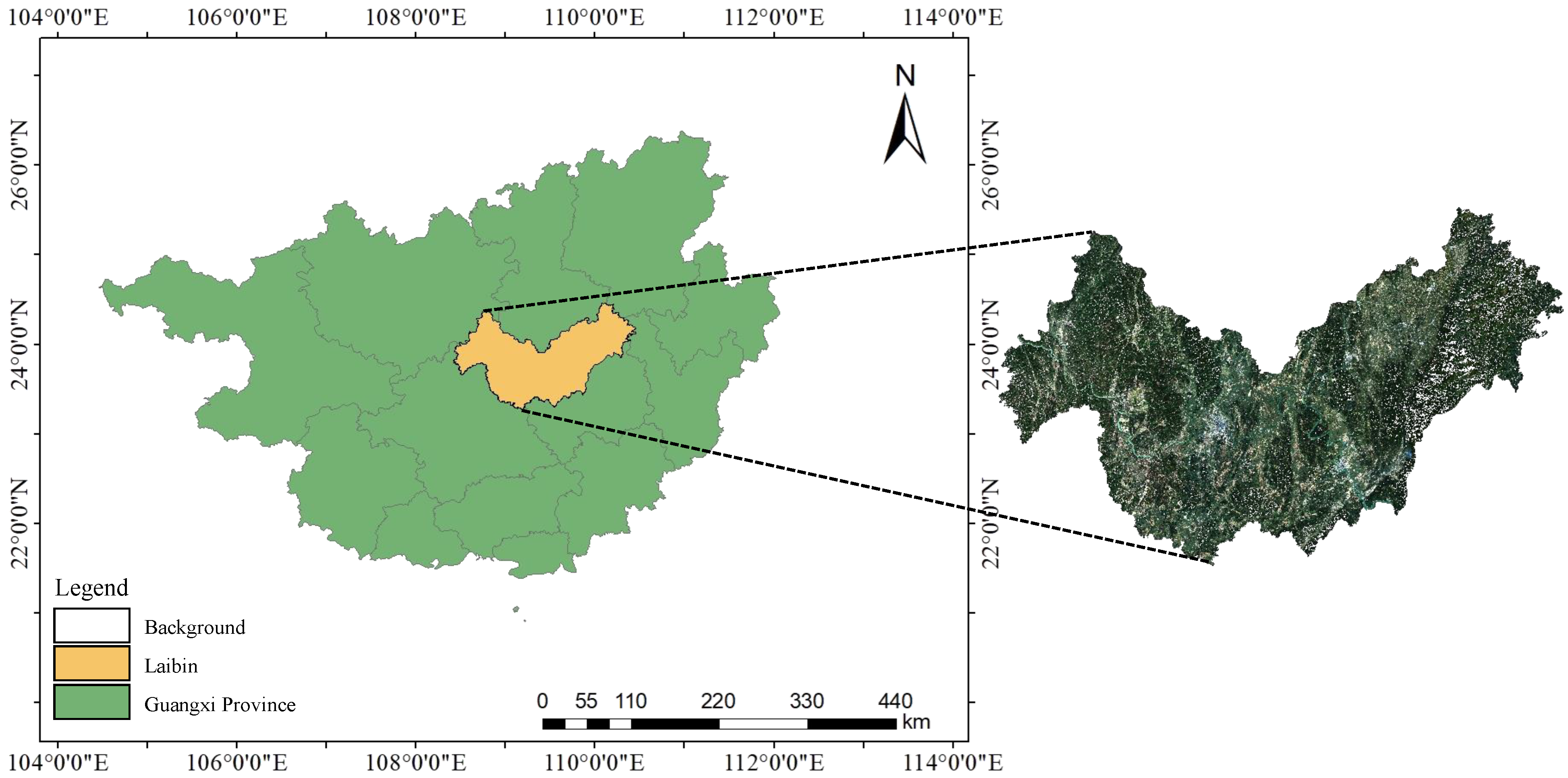
(2) Land cover in Laibin City, Guangxi Zhuang Autonomous Region, is classified using 10 m resolution public optical satellite images, and three public hyperspectral datasets are selected to test the generalizability of the classification model.

(3) The Forest, Sugarcane, and Rice areas of Laibin City, Guangxi Zhuang Autonomous Region, the study area, are taken as the focused areas for land use analyses.

The structure of this paper is shown as follows: Section 2 describes the study area and the data; Section 3 introduces the land cover classification algorithm proposed in this paper, the HCRNN; Section 4 consists of analyzing the experimental results and comparing them with various methods; and Section 5 presents the conclusions of this paper and the outlook for future work.

2. Study Area and Datasets

2.1. Study Area Overview

In this paper, the city of Laibin in the Guangxi Zhuang Autonomous Region is selected as the study area, which has coordinates ranging from 108°24′–110°28′ E to 23°16′–24°29′ N, with a total land area of 13,411 square kilometers [40]. The region presents a hilly and mountainous landscape with rolling mountain ranges and complex topography. The soil thickness is approximately 50 cm, and it falls within the subtropical monsoon climate zone. The climate is warm and humid in summer under the influence of the monsoon circulation, which is mainly characterized by sea-phase air masses; in winter, it is more influenced by cold and dry continental air masses. The summer is long, and the winter is short. The rainfall and temperature display contemporaneity. The climatic and soil conditions in Laibin are highly conducive to the growth and sugar accumulation of sugarcane. Consequently, sugarcane is one of the predominant crops in the Guangxi region, with the cultivated area accounting for approximately 60% of the country’s total. Accurate and efficient estimation of sugarcane acreage is of the utmost importance for local agricultural development, precision management, and yield estimation. The geographical location of the study area is indicated in Figure 1.

(1) Image Preprocessing

The 10 m resolution data of Laibin City, Guangxi Zhuang Autonomous Region, acquired by Sentinel-2 photography in 2017, 2019, and 2021, are used in this study, and the data in this paper are from the European Space Agency’s data storage server. Sentinel-2 is an optical remote sensing satellite with a wide-range, high-resolution, multispectral imaging mission, carrying a multispectral instrument (MSI) that can cover 13 spectral bands covering visible (VNIR), near-infrared (NIR), and short-wave infrared (SWIR), and has the uniqueness of containing three bands of data in the red-rimmed range, which provides a new source of data for classifying and counting the features in Laibin, Guangxi.

In processing the data, Sen2Cor-02.10.01 software (available for download from https://step.esa.int/main/snap-supported-plugins/sen2cor/, accessed on 16 June 2022) was first applied to perform radiometric calibration, atmospheric correction, terrain correction, and cirrus correction on Level-1C data to improve the quality of remote sensing images. Next, the SNAP 8.0 software (available for download from https://step.esa.int/main/download/snap-download/, accessed on 16 September 2021) was applied to resample the resolution of the bands to 10 m. Finally, the 13 bands were sorted in the order in the ENVI 5.6 software, and then waveband synthesis was performed. The image stitching was completed using the seamless mosaic tool, and then the TIFF-formatted Laibin City, Guangxi Zhuang Autonomous Region image data was exported.

(2) Sample Collection

In this paper, we obtained sample bank data from Laibin City, Guangxi Zhuang Autonomous Region, by collecting field data from the study area and labeling the region of interest (ROI) using ENVI 5.6 software. The main feature types in the study area include seven categories: sugarcane, forest, water, buildup, bareland, rice, and otherland. Samples were selected by using a GPS camera for field acquisition of selected pure sample areas in the study area, and then these samples were projected into the image and combined with expert empirical data for sample selection. A total of 24,818 feature-type sample points were obtained. During field collection of the sugarcane and rice samples, priority was given to the selection of contiguous planting areas with an area larger than 100 square meters to obtain data for the accumulation of a priori knowledge and later accuracy verification. Through these data collection methods, a more comprehensive and accurate understanding of the distribution of features in the study area can be obtained, providing data support for subsequent feature classification studies. The details of the sample library in the study area are shown in

Table 1. Sample size of the Laibin dataset.

Class No.	Class Name	2017 Laibin		2019 Laibin		2021 Laibin
		Training	Testing	Training	Testing	Training	Testing
1	Buildup	531	4779	585	5267	455	4100
2	Forest	991	8925	1029	9264	903	8133
3	Water	391	3521	311	2802	271	2447
4	Bareland	24	225	59	533	55	499
5	Sugarcane	188	1701	251	2260	116	1047
6	Rice	16	152	17	162	17	158
7	Otherland	337	3037	216	1948	324	2922
	Total	2478	22,340	2468	22,236	2141	19,306

; each category has a standard training and testing set. A total of 10% of the samples in each category are randomly selected as the training set, and the remaining 90% of the samples are used as the testing set. The information for the 13 bands of Sentinel-2 is shown in

Table 2. Sentinel-2’s 13 bands of information.

Band	Spatial Resolution (m)	Central Wavelength (nm)	Description
B1	60	443	Ultra blue (Coastal and Aerosol)
B2	10	490	Blue
B3	10	560	Green
B4	10	665	Red
B5	20	705	Visible and Near Infrared (VNIR)
B6	20	740	Visible and Near Infrared (VNIR)
B7	20	783	Visible and Near Infrared (VNIR)
B8	10	842	Visible and Near Infrared (VNIR)
B8a	20	865	Visible and Near Infrared (VNIR)
B9	60	940	Short Wave Infrared (SWIR)
B10	60	1375	Short Wave Infrared (SWIR)
B11	20	1610	Short Wave Infrared (SWIR)
B12	20	2190	Short Wave Infrared (SWIR)

.

2.2. Hyperspectral Data Description

In order to discuss whether the model proposed in this paper has high accuracy and better qualitative results for land cover classification on multiple-satellite remote sensing image products with universal and generalizability, in the experiments of this paper, we selected three hyperspectral publicly known available datasets. The Houston data, Indian Pines data, and Pavia University data are described below.

(1) The Houston data: The first set of data is a hyperspectral image of the University of Houston and the surrounding areas in Texas, USA, acquired by the ITRES CASI-1500 sensor. The dataset was provided by the NSF-funded National Center for Airborne Laser Mapping (NCALM) at the University of Houston. The image size is 349 × 1905 pixels and contains 144 bands. The spectral range is between 364 nm and 1046 nm, and the spatial resolution of the image is 2.5 m.

Table 3. Training and testing sets for different categories in the Houston dataset.

Class No.	Class Name	Training	Testing
1	Healthy Grass	198	1053
2	Stressed Grass	190	1064
3	Synthetic Grass	192	505
4	Tree	188	1056
5	Soil	186	1056
6	Water	182	143
7	Residential	196	1072
8	Commercial	191	1053
9	Road	193	1059
10	Highway	191	1036
11	Railway	181	1054
12	Parking Lot1	192	1041
13	Parking Lot2	184	285
14	Tennis Court	181	247
15	Running Track	187	473
	Total	2832	12,197

shows the category labels of the different categories in the sample bank of this dataset, as well as the samples that are divided into the training set and the testing set.

(2) Indian Pines data: The second set of data was acquired in 1992 using the Airborne Visual Infrared Imaging Spectrometer (Aviris) in the Indian Pines region of northwestern Indiana, USA. The total size of the image data is 145 × 145 pixels with a spatial resolution of 20 m, covering a spectral range of 400–2500 nm with 220 bands. However, special attention should be paid to the fact that from the 104th to the 108th, from the 150th to the 163rd, and the 220th bands are identified as noisy bands and are therefore eliminated from the subsequent analysis; the remaining 200 bands are finally used for the study.

Table 4. Training and testing sets for different categories in the Indian Pines dataset.

Class No.	Class Name	Training	Testing
1	Corn Notill	50	1384
2	Corn Mintill	50	784
3	Corn	50	184
4	Grass Pasture	50	447
5	Grass Trees	50	697
6	Hay Windrowed	50	439
7	Soybean Notill	50	918
8	Soybean Mintill	50	2418
9	Soybean Clean	50	564
10	Wheat	50	162
11	Woods	50	1244
12	Buildings Grass Trees Drives	50	330
13	Stones Steel Towers	50	45
14	Alfalfa	15	39
15	Grass Pasture Mowed	15	11
16	Oats	15	5
	Total	695	9671

shows the category labels of the different categories in the sample bank of this dataset, as well as the samples that are divided into the training set and the testing set.

(3) Pavia University data: The third set of data consists of images acquired in 2003, in the city of Pavia, Italy, using the German Rosis-03 airborne reflectance optical spectral imager. The dimensions of this dataset are 610 × 340 pixels with a spatial resolution of 1.3 m. This dataset contains 115 spectral channels covering the wavelength range of 430–860 nm. Since 12 bands are affected by noise, we selected 103 noise-rejected bands for the classification study.

Table 5. Training and testing sets for different categories in the Pavia University dataset.

Class No.	Class Name	Training	Testing
1	Asphalt	548	6304
2	Meadows	540	18,146
3	Gravel	392	1815
4	Trees	524	2912
5	Metal Sheets	265	1113
6	Bare Soil	532	4572
7	Bitumen	375	981
8	Bricks	514	3364
9	Shadows	231	795
	Total	3921	40,002

shows the category labels of the different categories in the sample bank of this dataset, as well as the samples that are divided into the training set and the testing set.

3. Research Methods

The workflow of the method included the following steps: (1) preprocessing of the Sentinel-2 data, which focused on processing the raw data with corrections, radiometric corrections, atmospheric corrections, and geometric corrections to make the data more accurate and usable (please refer to Section 2.1 for details); (2) production of sample library data, which selected a certain number of areas with known land cover types, collected and labeled within these areas, and constructed the sample library data used to train the model (please refer to Section 2.1 for details); (3) training the model, using the CNN as a front-end to receive spectral information, and the RNN was responsible for processing and predicting the feature information output from CNN; and (4) prediction to realize the land cover-type images of Laibin City, Guangxi Zhuang Autonomous Region.

The structure of the HCRNN neural network proposed in this paper is shown in Figure 2, which achieves the pixel-level classification of multispectral remote sensing images by fusing the CNN and RNN modules. Firstly, the original 13-band information of Sentinel-2 is adjusted to the 1D multispectral sequence using the fully connected layer and reshaped into a 3D multispectral feature matrix. The 2D-CNN structure, consisting of four convolutional layers, is designed to extract multi-scale feature information and generate higher-level, robust feature representations. The size of the input features is adjusted using the stride size to capture deeper feature information. Then, the extracted 2D-CNN spatial feature information at each level was input into the corresponding RNN structure, which consisted of two GRU units. To facilitate the following information fusion operation and to avoid overfitting, the global average pooling is used to adjust the 2D-CNN feature information at each level to the same convolution size before inputting the spectral–spatial feature information of the 2D-CNN into the RNN. The RNN is more sensitive to time series information, so the structure that contains four parallel RNNs can utilize the feature information generated by each convolutional layer to extract the contextual information among them, and capture the dependencies between different bands in multispectral images, thus making the classification task more stable and effective. Finally, the pixel superposition of the four levels of feature information through the add operation enriches the amount of information under the image features and realizes the fusion summation of the features, and then the fused features are processed by the activation function ReLU and sent to the MLP Head for classification, which achieved the high-precision pixel-level multispectral remote sensing image classification. The ReLU introduced the nonlinearities as the activation function. The network structure makes full use of the advantages of CNNs and RNNs to better mine time series information as well as spatial features in spectral data.

3.1. Recurrent Neural Network

The recurrent neural network (RNN) has become a popular method for processing sequence data and is distinct from the feedforward neural network in that the RNN is able to use recurrent edges to connect the neurons to themselves, which allows the probability distributions of the sequence data to be modeled at different time steps [41]. Figure 3 shows the classical recurrent neural network (RNN) structure.

In multispectral image classification, give a sequence data $x=(x_1,x_2,\dots ,x_t)$, and include among these $x_t$, $t\in \{1,2,\dots ,t\}$. In general, the information at moment t is denoted as the input vector $x_t$, and the output of the hidden layer at the $t-th$ time step is denoted as $s_t$. The output of the hidden layer can be calculated using the following formula:

$$s_t=f(u{x}_t+w{s}_{t-1}+b_s),$$

(1)

The $s_t$ in Equation (1) denotes the hidden state of the current time step, $x_t$ denotes the input of the current time step, w is the weight matrix from the input to the hidden state, $w{s}_{t-1}$ is the weight matrix from the hidden state of the previous time step to the hidden state of the current time step, and $b_s$ is the bias vector.

The output layer can be represented as:

$$o_t=f(v{s}_t+b_o),$$

(2)

The v in Equation (2) is the weight matrix, and $b_o$ is the bias vector.

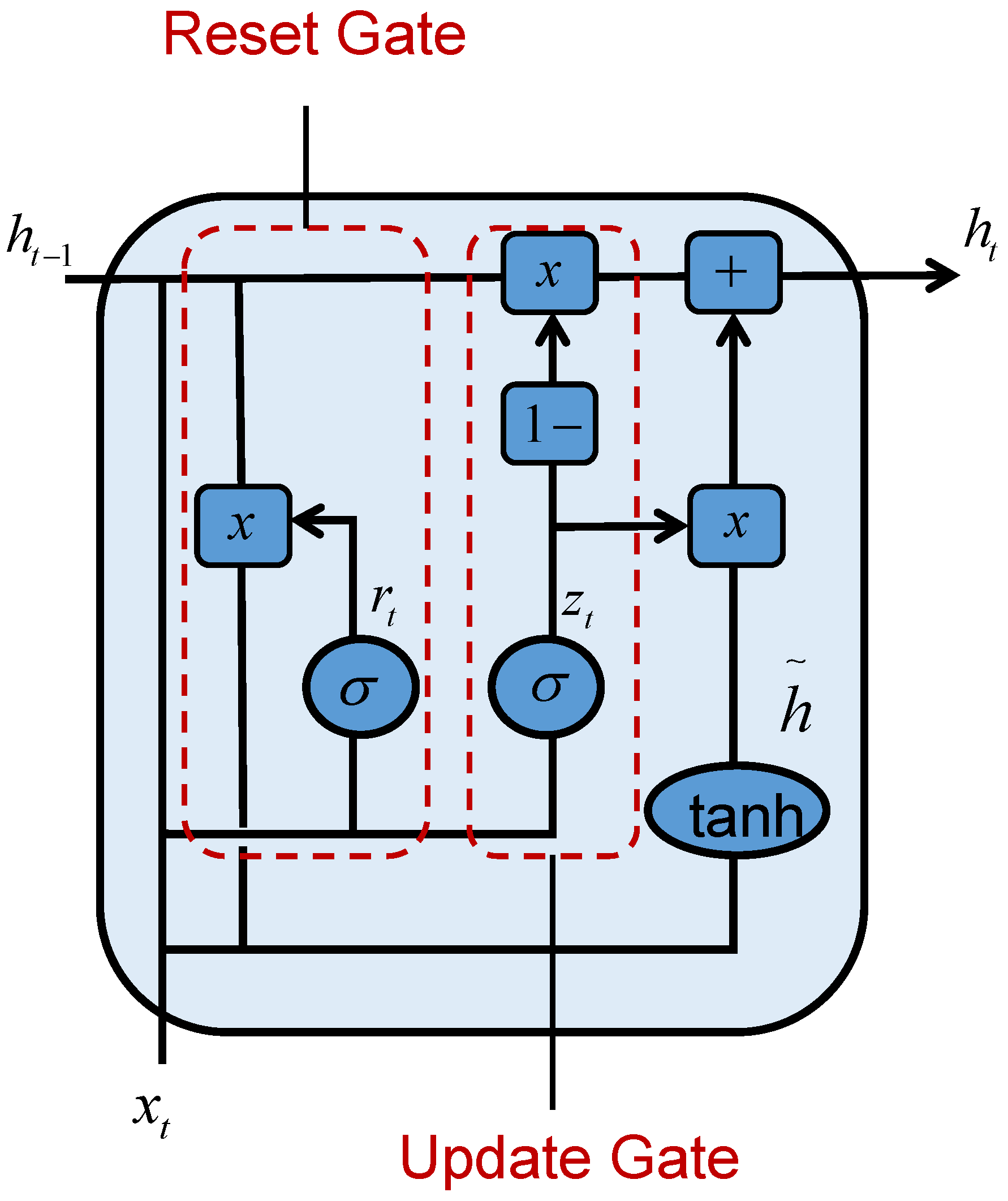
The RNN encountered the long-term dependency problem, i.e., it is difficult to train and process long-term sequential data because the gradient fades away as it propagates over time. To solve this problem, the LSTM [42] and GRU [43] were proposed. In comparison to the LSTM, the GRU has fewer parameters and can be trained faster or requires fewer data to generalize. Therefore, we choose the GRU to constitute the RNN module in our proposed framework. We can overcome the problem of vanishing gradient by using the GRU while reducing model complexity and training time. The RNN used in the experiments of this paper is composed of two GRU recurrent layers. The structure of the GRU is shown in Figure 4.

For the pixel-level input of the multispectral images, each pixel point in the image data is taken as an input in the form of $x_t$. The spatial feature vector of the image extracted by the 2D-CNN is taken as the hidden state of the previous time step of $h_{t-1}$ together with $x_t$ as the input to the GRU, thus realizing the pixel-level classification of multispectral images. The expressions for the reset gate and update gate are as follows:

$$r_t=\sigma (x_t{w}_r+u_r{h}_{t-1}+b_r),$$

(3)

$$z_t=\sigma (x_t{w}_z+u_z{h}_{t-1}+b_z),$$

(4)

where $\sigma (·)$ represents the logistic sigmoid function; $w_r$, $u_r$, $w_z$, and $u_z$ are the weight matrices; and $b_r$, $b_z$ represent the bias vectors in the neural network. $x_t$ is denoted as $s\times 1$ vectors in the pixel-level classification of multispectral images; s is the number of wavebands; and, in this paper’s experiments, we have chosen the number of wavebands to be 13, i.e., $s=13$.

The formula for calculating the candidate’s hidden state is:

$$\tilde{h}=tanh(w_{\tilde{h}}{x}_t+u_{\tilde{h}}(r_t\odot h_{t-1})+b_{\tilde{h}}),$$

(5)

In Equation (5), $tanh(·)$ represents the hyperbolic tangent function, $w_{\tilde{h}}$, $u_{\tilde{h}}$ are the weight matrices, and $b_{\tilde{h}}$ represents the bias vector. This part integrates the spectral feature information stored in the GRU, which needs to be combined with the information of the update gate for the next calculation of the hidden state:

$$h_t=z_t\odot h_{t-1}+(1-z_t)\odot \tilde{h},$$

(6)

In the GRU, the hidden state is passed to the output layer, and then the output layer computation at a time step t is expressed as:

$$y_t=h_t{w}_q+b_q,$$

(7)

where $w_q$ is the weight matrix, and $b_q$ represents the bias vector.

3.2. 2D-CNN

The convolutional neural network (CNN) was proposed by Yann Lecun of New York University in 1998 [44]. The convolutional neural network (CNN) is a deep learning model that is commonly used in image recognition, speech recognition, and other fields.

The following equation is applied to define the multispectral image in this paper: $X={\left\{x_i\right\}}_{i=1}^{H\times W\times 1}\in R^{H\times W\times C}$. In the above equation, $x_i\in R^{1\times 1\times C}$ represents the $i$-th pixel in the image, and H, W, and C represent the height, width, and number of bands of the multispectral image, respectively.

$$y_i=w{x}_i+b,$$

(8)

In this paper, w and b represent the weight matrix and bias vector of the fully connected layer, respectively. $x_i$ denotes the input 1D-pixel sequence, m is the output dimension of the fully connected layer, and $y_i$ represents the remodeling output with ${y_i}^{\prime }$, $y_i\in R^{1\times 1\times m}$, ${y_i}^{\prime }\in R^{n\times n\times \frac{m}{n^2}}$ where $m=13$ and $n=256$.

Throughout this section, we designed a 2D-CNN module as shown in Figure 5. Firstly, we used a fully connected layer to linearly stretch the input 1D pixel sequence to resize it into a 1D pixel sequence. To enhance the dimensionality and as an input to the 2D-CNN, we reshaped the 1D pixel sequence to a 3D pixel feature matrix. This stretch 2D-CNN module contains four convolutional layers. The first convolutional layer contains 32 convolutional kernels, the second convolutional layer contains 64 convolutional kernels, the third convolutional layer contains 128 convolutional kernels, and the last convolutional layer contains 256 convolutional kernels. In the selection of convolution kernels, except for the first convolutional layer, which uses a convolution kernel of size 1 × 1, the remaining three convolutional layers use a convolution kernel of size 2 × 2. With the above design, we can achieve feature extraction and increase the dimensions of the input image for better application in subsequent tasks.

3.3. Loss Function

Cross-entropy is a commonly used loss function that is particularly suitable for multi-classification problems. In deep learning, the cross-entropy loss function can be used to evaluate the difference between the model output results and the true labels and update and optimize the model parameters accordingly. With a separate calculation for each node, cross-entropy can effectively measure the difference between the probability distribution of the model output and the probability distribution of the true labels. During the model training process, the back-propagation algorithm is used to calculate the gradient, and the model parameters are continuously adjusted to minimize the cross-entropy loss function. Eventually, a classification model with high accuracy can be obtained by continuously optimizing the cross-entropy loss function. The expression is as follows:

$$L=\frac{1}{N}\sum _i{L}_i=-\frac{1}{N}\sum _i\sum _{c=1}^M{y}_{ic}log\left(p_{ic}\right),$$

(9)

where M represents the number of categories; $y_{ic}$ represents the sign function (0 or 1), taking 1 when the true category of sample i is equal to c, and 0 otherwise; and $p_{ic}$ is the predicted probability that the observation sample i belongs to category c.

3.4. Evaluation Metrics

A confusion matrix is a common method for evaluating the performance of classification models. For the multispectral pixel-level classification problem, the article used three confusion matrix-based evaluation metrics, namely, the accuracy rate, precision rate, and Kappa coefficient. The accuracy rate refers to the ratio of the number of samples correctly classified by the classifier to the total number of samples. The precision rate measures the percentage of samples that belong to a category out of all the samples classified by the classifier as belonging to that category. The Kappa coefficient, on the other hand, which considers the distribution of classification errors, is evaluated based on the classification consistency between samples. It is a more comprehensive and reliable indicator for model evaluation. The calculation of these three metrics is based on the confusion matrix, which can reflect the performance of the classifier more comprehensively. The three expressions are as follows:

$$Accuracy=\frac{TP+TN}{TP+FN+FP+TN},$$

(10)

$$Precision=\frac{TP}{TP+FP},$$

(11)

$$Kappa=\frac{P_o-P_e}{1-P_e},$$

(12)

In the above equations, $TP$ (true positive) is the number of samples correctly predicted to be positive, $FP$ (false positive) is the number of samples that are negative but incorrectly predicted to be positive, $TN$ (true negative) is the number of samples that are correctly predicted to be negative, $FN$ (false negative) is the number of samples that are positive but incorrectly predicted to be negative, $P_o$ is the overall classification accuracy, and $P_e$ is the expected consistency rate.

3.5. Experimental Setting

The experiments in this paper used ENVI software to obtain the coordinate point data of sample points and regions of interest collected outdoors and export them to text files as a dataset. During the model training, a batch size of 32, a maximum number of iterations of 300, and a learning rate decay multiplier of 0.9 were used. The experimental code is all implemented by Python 3.9 in PyTorch 1.10.2. The training environment for the model is Windows 11 + 12th Gen Intel(R) Core(TM) i5-12400F + NVIDA GeForce RTX 3060 GPU.

4. Results of the Experiment

The study area classification experiments in this paper are conducted using the data in Table 1, and the hyperspectral dataset classification experiments are conducted using Table 3, Table 4 and Table 5.

To evaluate the performance and effectiveness of our models, we selected SVM, KNN (k-nearest neighbor), RF (random forest), ViT (vision Transformer), SpectralFormer, 1D-CNN, an RNN, and the HCRNN for comparison on the study area Guangxi Laibin dataset, the Houston dataset, the Indian Pines dataset, and the Pavia University dataset.

(1) SVM: In the SVM model, the penalty factor is set to 10, which helps to limit model overfitting. Meanwhile, we use the radial basis function (RBF) as the kernel function to transform the SVM into a nonlinear model. When choosing the decision function, we use the “ovr” (one-vs.-rest) strategy to deal with multi-category classification problems.

(2) KNN: The number of nearest neighbors (the k value) is set to three, i.e., for each test data. The European distance is used as the distance metric.

(3) RF: Random forest with 100 trees.

(4) ViT: The structure of ViT is set up as five encoders. Each encoder’s module consists of four self-attentive layers, eight hidden layers of MLPs, and a dropout layer that suppresses 0% of the neurons, with an arbitrary grouping embedded in a spectral dimension of 64.

(5) SpectralFormer: The SpectralFormer module is designed with five encoder modules, each containing four self-attentive layers, eight hidden layers of MLPs, and a dropout layer that suppresses 10% of the neurons. The length of any group of spectral embedding vectors is 64.

(6) 1D-CNN: The 1D-CNN structure consists of a convolutional layer, a batch normalization layer, a maximum-pooling layer, a fully connected layer, an output layer, and a ReLU activation function.

(7) RNN: The structure of RNN is a two-layer gated recurrent unit (GRU).

(8) HCRNN: THe HCRNN model contains a CNN module and an RNN module. The fully connected layer of the CNN module has an input dimension of 13 and an output dimension of 256, which is transformed into an 8 × 8 × 4 3D feature matrix after the reshaping operation. The convolutional layers are set up as follows: the first convolutional layer has 32 convolutional kernels, the second convolutional layer has 64 convolutional kernels, the third convolutional layer has 128 convolutional kernels, and the last convolutional layer has 256 convolutional kernels. The RNN module consists of two layers of GRUs.

4.1. Comparative Analysis of Multiple Methods

In this section, we compared the proposed method with other representative and advanced models to obtain the corresponding qualitative results.

Table 6. Classification results of different classification methods on the Laibin 2017 dataset. The best results for each row are shown in bold.

Class No.	Method
	SVM	KNN	RF	1D-CNN	ViT	SpectralFormer	RNN	HCRNN
1	94.89	90.83	94.56	91.80	96.00	95.40	95.33	97.09
2	98.42	98.10	98.88	98.30	99.04	99.31	98.92	99.22
3	96.39	96.45	95.60	95.80	97.61	97.13	96.96	98.35
4	100.00	96.44	92.89	93.33	100.00	99.56	99.11	100.00
5	79.19	85.89	84.30	72.03	90.65	90.83	88.18	92.83
6	28.29	33.55	39.47	37.50	71.05	69.74	69.08	78.95
7	95.92	91.77	92.10	89.06	90.18	93.94	91.64	96.34
OA (%)	95.08	94.04	94.94	92.79	96.14	96.55	95.84	97.62
AA (%)	84.73	84.72	85.40	82.54	92.08	92.27	91.32	94.68
Kappa	0.9340	0.9201	0.9321	0.9031	0.9482	0.9538	0.9442	0.9681

gives the classification results of different models on the study area dataset with quantitative classification accuracies, OA, AA, and Kappa. Table 6 shows the classification results of the 2017 Laibin dataset with different classification methods. In general, 1D-CNN performs the worst. The qualitative indexes’ OA, AA, and Kappa values are the lowest among all the classification methods, 92.79%, 82.54%, and 0.9031, respectively, and, for sugarcane and rice, the classification ability is weaker, only 72.03% and 37.50%. The reason for the poor classification effect of 1D-CNN on multispectral data is probably because multispectral data have multiple dimensions spatially, whereas 1D-CNN can only learn and extract features from the data in one dimension, which cannot make full use of the spatially rich information of multispectral data. SVM, KNN, and RF are traditional machine learning classification algorithms, and their classification performances are comparable as measured by the qualitative metrics OA, AA, and Kappa. The OA of SVM is 95.08%, the AA is 84.73%, and the Kappa is 0.9340, and the classification ability for rice is the worst among all of the compared methods with only 28.29%, but, in the classification performance for bareland, SVM achieves a classification accuracy of 100%, which is the best result among all of the classification methods. The classification methods for deep learning are ViT, SpectralFormer, the RNN, and our proposed HCRNN algorithm in addition to the 1D-CNN analyzed above. ViT also achieves a promising classification performance for bareland, with a classification accuracy of 100%, and SpectralFormer has the best classification ability of all classification methods for forest, with a classification accuracy of 99.31%. However, our proposed HCRNN algorithm outperforms the other models on the 2017 dataset, achieving an OA of 97.62%, an AA of 94.68%, and a Kappa value of 0.9681. The HCRNN has the best classification performance for the six feature classes of buildup, water, bareland, rice, sugarcane, and otherland with classification accuracies of 97.09%, 98.35%, 100%, 92.83%, 78.95%, and 96.34%, respectively. Our combined model algorithm, the HCRNN, compares favorably with the single RNN model with improvements in buildup (+1.76%), water (+1.39%), sugarcane (+4.65%), rice (+9.9%), and otherland (+4.7%). Undoubtedly, the HCRNN algorithm is better at mining time series information as well as spatial features in spectral data, and its classification accuracy is better than other methods.

The land cover-type maps of different classification methods to classify the city of Laibin in Guangxi are shown in Figure 6. We marked and magnified the red boxes of the classification map based on the sample points information obtained from fieldwork and prior knowledge. In the red boxes are buildup, forest, water, bareland, sugarcane, rice, and otherland. 1D-CNN has a poor classification performance overall, but, for the better-differentiated categories (e.g., buildup, water, etc.), the differentiation is also higher. However, 1D-CNN is confused when facing indistinguishable categories, e.g., mistakenly detecting rice in categories such as bareland and otherland. SVM performs poorly in distinguishing rice and bareland and is prone to recognition errors in localized areas. Four deep learning classification models, ViT, SpectralFormer, the RNN, and the HCRNN are chosen for our experiments, and they perform well in terms of overall classification results, being able to clearly extract the outlines of feature classes and better identify classes with smaller differences. However, we find that the HCRNN performs much better when observed on a local scale, and it is significantly better at identifying otherland and sugarcane than the other classification methods.

Now, we will discuss whether the model proposed in this paper has a high accuracy and better qualitative results for land cover classification of multiple-satellite remote sensing image products with universal and general applicability. In the Houston dataset, the Indian Pines dataset, and the Pavia University dataset, our proposed classification method is compared with other advanced and representative models to produce qualitative results. The classification results of different models on the Houston dataset, the Indian Pines dataset, and the Pavia University dataset with quantitative classification accuracies, the OA, AA, and, Kappa are given in

Table 7. Classification accuracy of different classification models in the Houston dataset. The best results for each row are shown in bold.

Class No.	Method
	SVM	KNN	RF	1D-CNN	ViT	SpectralFormer	RNN	HCRNN
1	82.53	83.19	83.57	84.24	84.14	83.38	83.29	85.09
2	98.68	96.15	98.40	97.56	92.76	97.37	98.12	95.77
3	99.01	99.60	98.02	99.60	98.81	99.41	99.41	99.41
4	97.63	98.30	97.16	98.48	96.12	97.92	98.11	90.44
5	95.93	96.69	96.31	97.06	96.40	97.25	95.08	96.50
6	74.13	94.41	97.20	99.30	94.41	99.30	97.02	95.10
7	82.56	83.58	76.49	89.27	76.77	75.40	76.49	81.92
8	30.48	48.91	38.08	73.41	47.77	47.10	38.08	63.44
9	78.94	69.69	71.67	72.71	72.99	68.84	71.67	65.34
10	27.41	70.46	66.41	67.47	47.68	52.32	66.41	77.12
11	87.29	81.50	75.33	83.11	80.46	80.55	75.33	75.14
12	36.12	50.62	60.61	65.32	40.92	52.16	60.61	75.98
13	29.47	41.75	51.58	58.95	44.91	46.32	51.58	65.26
14	97.98	98.38	100.00	98.79	99.19	97.17	100.00	98.79
15	98.10	98.10	91.54	97.67	98.94	98.52	91.54	98.10
OA (%)	73.63	79.42	77.59	84.15	75.82	77.31	78.07	82.32
AA (%)	74.42	80.76	80.41	85.53	78.15	79.56	80.19	84.23
Kappa	0.7141	0.7769	0.7625	0.8280	0.7383	0.7541	0.7625	0.8084

,

Table 8. Classification accuracy of different classification models in the Indian Pines dataset. The best results for each row are shown in bold.

Class No.	Method
	SVM	KNN	RF	1D-CNN	ViT	SpectralFormer	RNN	HCRNN
1	37.07	56.14	58.38	62.64	47.98	62.57	73.63	63.29
2	20.41	53.70	57.65	42.73	38.90	62.37	42.98	73.34
3	76.09	77.17	82.61	89.67	71.74	91.85	27.72	88.59
4	45.19	80.71	84.79	82.10	76.06	88.14	24.38	75.62
5	79.34	77.33	79.91	82.64	72.45	86.08	79.91	80.49
6	98.86	94.99	95.90	96.13	95.67	96.58	97.27	95.22
7	52.94	62.96	75.71	72.98	57.52	71.68	6.97	83.22
8	53.35	43.67	59.10	65.22	30.07	72.70	42.18	71.22
9	24.29	45.04	57.80	65.07	25.18	62.77	18.44	82.27
10	98.77	94.44	95.68	96.91	95.68	98.77	91.98	98.77
11	96.06	73.55	88.10	91.88	69.21	93.89	93.89	84.24
12	11.82	35.15	56.67	62.42	18.48	49.09	26.06	73.03
13	91.11	97.78	97.78	100.00	95.56	100.00	97.78	97.78
14	0.00	79.49	56.41	74.36	17.95	71.79	28.21	94.87
15	0.00	81.82	81.82	63.64	45.45	90.91	18.18	90.91
16	0.00	80.00	100.00	100.00	40.00	100.00	80.00	100.00
OA (%)	55.32	60.56	69.66	71.74	50.64	75.38	53.27	76.79
AA (%)	49.08	71.40	76.77	78.03	56.12	81.20	53.10	84.55
Kappa	0.4916	0.5564	0.6576	0.6787	0.4486	0.7192	0.4673	0.7365

and

Table 9. Classification accuracy of different classification models in the Pavia University dataset. The best results for each row are shown in bold.

Class No.	Method
	SVM	KNN	RF	1D-CNN	ViT	SpectralFormer	RNN	HCRNN
1	70.11	75.52	80.44	73.89	64.70	75.21	79.92	76.59
2	73.98	61.18	53.90	82.04	65.74	69.43	72.21	83.81
3	30.03	52.78	46.39	66.94	53.11	71.46	63.47	60.88
4	98.70	96.77	98.49	95.88	96.02	97.91	98.11	96.12
5	99.37	99.37	98.65	99.37	99.28	99.01	98.47	99.46
6	35.28	69.20	76.22	72.35	51.66	67.61	78.26	78.30
7	89.30	83.89	78.90	93.58	91.34	92.15	82.10	93.27
8	93.25	84.42	89.77	91.97	77.50	77.44	87.51	92.69
9	99.87	96.10	97.36	99.87	99.87	99.50	96.48	96.60
OA (%)	71.97	70.83	69.28	81.93	68.83	74.95	78.35	83.57
AA (%)	76.65	79.92	80.01	86.21	77.69	83.30	84.05	86.41
Kappa	0.6320	0.6323	0.6196	0.7628	0.6018	0.6797	0.7223	0.7847

. The data in bold in each row is the best result of classification for each category. From Table 9, it can be concluded that as a whole ViT is the worst (the OA, AA, and Kappa are all lower than the other models), but interestingly, ViT has the best classification ability for shadows with 99.87%; meanwhile, SVM and 1D-CNN also have 99.87% classification accuracy for shadows. Figure 7, Figure 8 and Figure 9 indicate the classification maps obtained from different classification models on the Houston dataset, the Indian Pines dataset, and the Pavia University dataset.

Overall, the traditional classifiers RF, KNN, and SVM appear to have similar classification performances on all three hyperspectral datasets, i.e., they are all ordinary in qualitative evaluation, with the OA, AA, and Kappa values in the lower-middle range of all the classifiers. However, their performance is more prominent in the individual classification categories. SVM has the highest classification accuracy in the Houston dataset for the categories of stressed grass, road, and railway with 98.68%, 78.94%, and 87.29%, respectively. RF even achieves 100% classification accuracy for the category of tennis court in the Houston dataset. Deep learning has powerful learning skills, the recurrent neural network (RNN) and SpectralFormer perform more prominently, and the three qualitative metrics of OA, AA, and Kappa are higher than the traditional classifiers on both the Houston dataset and the Pavia University dataset. However, in the Indian Pines dataset, the RNN has an overfitting problem for soybean notill, a category with more training and testing samples, which results in a classification accuracy of only 6.97% but still reflects the superiority of deep learning in land cover classification. 1D-CNN is more excellent at capturing spatial features in a large number of continuous spectral data, such as hyperspectral data, so 1D-CNN performs well in the three hyperspectral datasets, especially in the Houston dataset where OA, AA, and Kappa are the highest values among all classification methods. The HCRNN algorithm proposed in this paper can better mine the time series information as well as the spatial features in the spectral data, and its classification accuracy is better than the other methods, with the highest OA, AA, and Kappa values in the Indian Pines dataset and the Pavia University dataset. Additionally, for categories with a small number of training samples, such as alfalfa, oats, and grass pasture mowed, in the Indian Pines dataset, the HCRNN presents a better performance capability, with classification accuracies of 94.87%, 100%, and 90.91%. 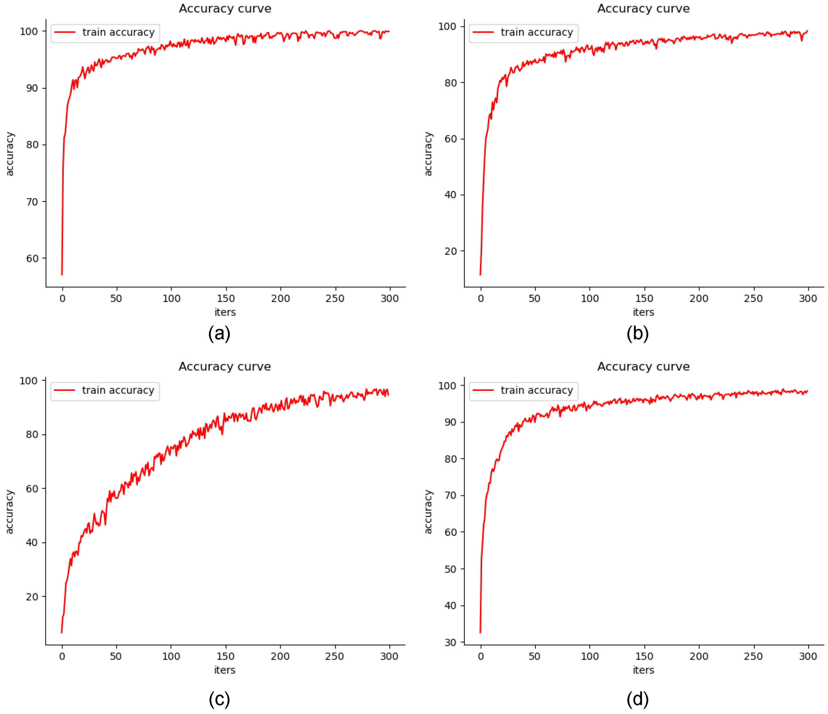Figure 10 and Figure 11 show the accuracy curves and loss curves of the HCRNN during training on the four datasets.

4.2. Analysis of Land-Use Change in the Study Area

In this paper, the land cover classification of Laibin was carried out using Sentinel-2 series imagery for 2017, 2019, and 2021, downloaded from the official ESA website (https://scihub.copernicus.eu, accessed on 3 February 2023). After the preprocessing operation of the image data (please refer to Section 2.1 for details), the ENVI software was used to mark the region of interest (ROI) of the sample data collected in the field, and the ROI coordinate point data were exported to text files. The training and testing sets were divided using a ratio of 1:9. Table 1 shows the sample data for the years 2017, 2019, and 2021. The algorithm proposed in this paper was used to classify the land cover, analyze the land use changes, and compare and analyze with the previously accumulated classification knowledge and models. Focused analyses of forest, rice, and sugarcane in Laibin were conducted, and we delineated these portions of the area as the key areas of focus for the region. The analysis of changes in these areas enables a better understanding of the distribution of forests and agricultural production in the region. According to the data in Table 6,

Table 10. Classification results of different classification methods on the Laibin 2019 dataset. The best results for each row are shown in bold.

Class No.	Method
	SVM	KNN	RF	1D-CNN	ViT	SpectralFormer	RNN	HCRNN
1	98.35	98.01	99.30	96.81	99.11	99.13	98.99	98.93
2	97.87	95.65	97.31	93.87	97.19	97.88	97.01	99.03
3	97.47	97.89	97.32	96.25	97.64	98.64	97.04	98.07
4	93.06	97.00	92.50	93.25	93.80	95.86	95.31	97.56
5	87.7	88.89	86.81	84.44	89.77	85.42	89.54	91.50
6	70.99	75.93	67.28	65.22	80.86	76.54	72.84	74.07
7	74.08	80.34	77.05	71.84	81.20	88.49	81.39	89.09
OA (%)	94.50	94.35	94.61	91.76	95.34	95.98	95.14	97.03
AA (%)	88.50	90.53	88.23	85.95	91.37	91.71	90.93	92.61
Kappa	0.9247	0.9232	0.9262	0.8877	0.9366	0.9452	0.9337	0.9596

, and

Table 11. Classification results of different classification methods on the Laibin 2021 dataset. The best results for each row are shown in bold.

Class No.	Method
	SVM	KNN	RF	1D-CNN	ViT	SpectralFormer	RNN	HCRNN
1	96.27	94.32	96.31	94.60	95.09	95.36	95.12	96.49
2	92.99	90.95	90.42	91.32	94.22	96.03	93.99	96.64
3	96.46	96.51	95.64	94.59	97.32	96.93	97.66	97.80
4	71.53	79.36	73.67	57.47	74.73	87.54	89.50	93.42
5	92.69	89.91	91.42	85.70	85.83	91.86	87.45	89.57
6	16.06	38.32	14.60	1.82	69.23	64.47	46.52	73.26
7	63.86	68.34	71.12	49.55	78.98	71.84	75.63	85.95
OA (%)	89.03	88.51	88.97	84.43	90.85	91.58	90.70	93.93
AA (%)	75.69	79.67	76.17	67.87	85.06	86.29	83.70	90.45
Kappa	0.8600	0.8541	0.8598	0.8002	0.8836	0.8629	0.8818	0.9230

, it can be concluded that the HCRNN algorithm is the best at classifying the Sentinel-2 images of Laibin City for the years 2017, 2019, and 2021. Therefore, land use change in Laibin City was analyzed in this section using the classification proposed in this article.

The classification results obtained by the different classification methods on the datasets of Guangxi Laibin City for the years 2017, 2019, and 2021 are shown in Table 6, Table 10, and Table 11. It is possible to clearly and unambiguously conclude that the qualitative results of the classification of the HCRNN model for all three phases of the city of Laibin, in Guangxi, are optimal. The HCRNN has OA values of 97.62%, 97.03%, and 93.93% in the 2017, 2019, and 2021 datasets, respectively. In comparison to the classification performance of a single RNN model, the HCRNN improves the OA values by 1.78%, 1.89%, and 3.23% over the RNN. For the focused forest region, the HCRNN performs well in the 2017 Laibin dataset, and even better in the 2019 and 2021 Laibin datasets, i.e., it is the most prominent in classifying this category of forest, with the highest classification accuracy of all the classification methods. In the agricultural cultivation area, focusing on rice and sugarcane regions, rice and sugarcane had the highest classification accuracy of all classification methods on the 2017 Laibin dataset, with the sugarcane category having a more favorable classification performance in 2019, and the rice category having the optimal classification in 2021, in comparison with the remaining methods. As a result, it is more appropriate to use the land cover classification results of Laibin City obtained from the HCRNN for land-use change analysis.

It is concluded from

Table 12. Changes in land-use types in the Laibin City area, Guangxi, during the three years of 2017, 2019, and 2021.

Class No.	Class Name	Area (km2)			Area Change Rate (%)
		2017	2019	2021	2017–2019	2019–2021	2017–2021
1	Buildup	848.1643	680.2361	957.4973	−19.80	40.80	12.89
2	Forest	7997.1016	8990.4149	8103.0020	12.42	−9.87	1.32
3	Water	456.4951	249.7476	377.0088	−45.29	−50.95	−17.41
4	Bareland	140.5018	131.5372	125.2932	−6.38	−4.75	−10.82
5	Sugarcane	832.3258	965.4852	1546.5997	14.92	60.76	85.82
6	Rice	110.5949	184.1268	164.9849	66.49	−10.40	49.18
7	Otherland	2988.1359	2171.7716	2098.9335	−27.32	−3.35	−29.76

that the area occupied by the forest area is the largest in the city of Laibin, followed by otherland. The extent of the area covered by buildup varied considerably over the three years. The area of buildup is mainly concentrated around the areas of active agricultural cultivation in the central part of the city of Laibin, with a growing trend in general. The area covered by bareland is a small proportion of the size of the city of Laibin. It is mainly concentrated in the vicinity of the buildup area. The bareland region has seen a relatively small change in area, showing a downward trend from year to year over the three years. The water area is extensive in the city of Laibin, with the river spanning the entire city of Laibin, covering an area range that appears to be decreasing and then increasing over the three years and still showing an overall decreasing trend. The reason for this phenomenon may be attributed to the fact that there has been less rain and a significant increase in extreme weather in recent years. The type of crop cultivation in Laibin City mainly includes sugarcane and rice. The area range covered by sugarcane is increasing year by year, and the area range covered by rice shows an expansion and then a decline, but the overall observation is that it is still increasing. The detailed land cover distribution map of Laibin City is shown in Figure 12.

The vegetation cover type of Laibin City is mainly forest, sugarcane, and rice. To better monitor the vegetation change and understand the ecological development, we considered the forest, sugarcane, and rice areas as the focus areas of the study in this region. In the spatial feature distribution maps of forest, rice, and sugarcane in Laibin City, the other feature categories were unified in the same color, as shown in Figure 13. It is clear from the graph that the forest and rice areas had the largest acreage in 2019 of the last three years, while the sugarcane area had the largest planting acreage in 2021 of the last three years. An in-depth study of the changes in these key areas can help us better understand the trends in land resource use and changes in the region, further promoting optimization of resource allocation, balance in ecological development, and enhancement of agricultural and plantation production capacity. The land use analyses of forest, rice, and sugarcane have significant implications for achieving sustainable development and ecological protection in Laibin City.

In Table 12, we analyze the change in land-use types in the Laibin City area of Guangxi during the three years of 2017, 2019, and 2021. For the forest area, which has the largest coverage, the change in area is relatively small, with 7997.1016 km² in 2017, and a three-year peak of 8990.4149 km² in 2019, which is an increase of 12.42% compared to 2017. The area covered by forest area was 8103.0020 km² in 2021, which is a decrease of 9.87% in comparison with 2019, but still shows a small increase in comparison with the area covered in 2017, with an improvement of 1.32%. This may be due to the call to return farmland to forests in recent years, so the forest area still shows an increasing trend. The gradual expansion of sugarcane cultivation areas to fulfill the needs of the development of the agricultural economy in Laibin City is probably the reason for the reduction of forest cover during a short period in the year 2021. The cultivated rice area was 110.5949 km² in 2017, 184.1268 km² in 2019, and 164.9869 km² in 2021. The rate of change in the area under cultivation for rice improved by 66.49% from 2017 to 2019 and then decreased by 10.40% from 2019 to 2021, compared to 2017–2021, when the rice area under cultivation was still growing, improving by 49.18%. It is possible that due to the advancement of modernization of food crops in Laibin in recent years, the cultivation range is wider than before, so the rice cultivation area shows a substantial increase in 2017–2019, and the agricultural cultivation area is more stable. Therefore, this may be the reason for a slight decline in rice acreage in 2019–2021. The sugarcane region is more variable in terms of acreage. The cultivation area for sugarcane is 832.3258 km² in 2017, which increases to 965.4852 km² in 2019, and further expands to 1546.5997 km² in 2021. The growth rate of the cultivation area for sugarcane has shown improvement over these years, with a 14.92% increase from 2017 to 2019, a 60.76% increase from 2019 to 2021, and a substantial 85.52% increase from 2017 to 2021. This is due to the vigorous development of modern characteristic agriculture in Laibin City in recent years, and the climate and soil conditions in Laibin City are suitable for cultivating sugarcane. The annual sugarcane production in Laibin City can account for one-eighth of China’s total sugarcane production. Sugar production in Laibin City in 2021 has reached another historical high, which proves that the area of sugarcane cultivation has changed so much and grown so rapidly. Figure 14 shows the dynamics of forest, rice and sugarcane in Laibin City over three years.

4.3. Analysis of Samples with Different Proportions

In order to assess the impact of the small number of training samples on the experimental results, in this paper, we randomly selected different proportions of training samples from a given dataset in our sample data of Laibin City in 2017, 2019, and 2021, and run it nine times with 10%, 20%, …, 90% intervals of 10%, and the remaining samples in each run were used as the testing set without setting up the validation set. The classification accuracies obtained by the HCRNN algorithm proposed in this paper with different proportions of training samples in the 2017, 2019, and 2021 Laibin data are shown in Figure 15. As the training samples increase, the classification accuracy becomes higher and higher, while the noise gradually decreases. For example, when the proportion of training samples reaches 70%, 80%, and 90%, the classification accuracy is further improved, and the OA value stabilizes more and more, which shows that the HCRNN algorithm is reliable.

4.4. Discussion

In this article, the Sentinel-2 image data of Laibin City was selected for the experiments, and all 13 bands were included to achieve the land cover classification of the study area. The aim is to obtain more complete information about the land, which will help to achieve a more detailed and comprehensive classification of features for the identification of the different land cover types. Meanwhile, 13 bands are selected so that we can also flexibly combine them according to different classification requirements. In the study area dataset and the three hyperspectral public datasets, the traditional classification methods SVM, KNN, and RF, and the deep learning classification methods 1D-CNN, ViT, SpectralFormer, the RNN, and the HCRNN present different experimental results. SVM and RF have the advantage of lower computational cost and the ability to handle relatively complex classification tasks with fewer training samples [45]. However, their classification performance is not superior enough when compared to deep learning methods such as RNN and SpectralFormer, which are good at capturing deep feature information, such as sequences [46]. In multispectral datasets, the performance of SVM and RF is not outstanding compared to the RNN and SpectralFormer in deep learning methods. KNN can learn from a limited number of samples to complete the classification task, but KNN is similarly not sensitive enough to sequence information [47] and performs moderately well in experiments. 1D-CNN is widely used in problems related to time series and is better at capturing spatial features in large amounts of continuous spectral data, such as hyperspectral data [48]. Thus, 1D-CNN performs well in the three hyperspectral datasets, with the best classification performance in the Houston dataset. The reason for the weak performance in multispectral data may be that multispectral data has multiple dimensions in space, whereas 1D-CNN can only learn and extract features from one dimension of the data. ViT still outperforms traditional methods in multispectral datasets due to its ability to long-term dependence on modeling [49]. In contrast, although the RNN can process time-series data in multispectral remote sensing images, it does not work as well as the HCRNN which combines a CNN and an RNN, when the RNN is used alone.

Based on the experimental results presented in this paper, it can be concluded that the proposed HCRNN model outperforms the other classification methods in achieving pixel-level classification of Sentinel-2 remote sensing images. The HCRNN model exhibits the best classification performance in the multispectral dataset and produces good results in the three hyperspectral datasets, demonstrating its reliability and universality in different scenarios. However, it is worth noting that the HCRNN model has a larger number of parameters due to the extraction of multi-scale features. As a result, the computation time is longer, and the computation cost is higher than single deep learning classification models, such as a CNN or an RNN. Therefore, it is essential to explore more efficient methods of combining a CNN and RNN, which will be a focus of future work.

5. Conclusions

In this study, the city of Laibin, Guangxi Zhuang Autonomous Region, is used as the study area, and the Sentinel-2 series of images from 2017, 2019, and 2021 are utilized to classify the features. We proposed a multispectral remote sensing image classification model fusing a CNN and RNN, which improves the classification accuracy and realizes pixel-level classification by extracting feature information at four levels of the 2D-CNN module as the input to the RNN, ensuring that the effective feature information is delivered to deeper levels. The experimental results show that our network structure is superior to traditional models and other deep learning models in land cover classification, which provides a new technical model with practical significance for agricultural monitoring. However, the 2D-CNN module designed in this paper is relatively simple, and, in future work, we can continue to explore ways to upgrade the dimension of 1D pixel feature sequences into 2D or 3D pixel feature matrices to enrich the feature information and enhance the diversity of features. In addition, the recently proposed Transformer model also performs well in classification tasks on pixel sequences, so the fusion of 2D-CNN and Transformer can be considered to further improve the classification performance.