Article

Tree Species Classification over Cloudy Mountainous Regions by Spatiotemporal Fusion and Ensemble Classifier

1
College of Geo-Exploration Science and Technology, Jilin University, Changchun 130026, China
2
Flight Research Institute, Air Force Aviation University, Changchun 130022, China
*
Author to whom correspondence should be addressed.
Forests 2023, 14(1), 107; https://doi.org/10.3390/f14010107
Submission received: 7 November 2022 / Revised: 17 December 2022 / Accepted: 3 January 2023 / Published: 5 January 2023
(This article belongs to the Special Issue Mapping Forest Vegetation via Remote Sensing Tools)

Abstract

:
Accurate mapping of tree species is critical for the sustainable development of the forestry industry. However, the lack of cloud-free optical images makes it challenging to map tree species accurately in cloudy mountainous regions. In order to improve tree species identification in this context, a classification method using spatiotemporal fusion and ensemble classifier is proposed. The applicability of three spatiotemporal fusion methods, i.e., the spatial and temporal adaptive reflectance fusion model (STARFM), the flexible spatiotemporal data fusion (FSDAF), and the spatial and temporal nonlocal filter-based fusion model (STNLFFM), in fusing MODIS and Landsat 8 images was investigated. The fusion results in Helong City show that the STNLFFM algorithm generated the best fused images. The correlation coefficients between the fusion images and actual Landsat images on May 28 and October 19 were 0.9746 and 0.9226, respectively, with an average of 0.9486. Dense Landsat-like time series at 8-day time intervals were generated using this method. This time series imagery and topography-derived features were used as predictor variables. Four machine learning methods, i.e., K-nearest neighbors (KNN), random forest (RF), artificial neural networks (ANNs), and light gradient boosting machine (LightGBM), were selected for tree species classification in Helong City, Jilin Province. An ensemble classifier combining these classifiers was constructed to further improve the accuracy. The ensemble classifier consistently achieved the highest accuracy in almost all classification scenarios, with a maximum overall accuracy improvement of approximately 3.4% compared to the best base classifier. Compared to only using a single temporal image, utilizing dense time series and the ensemble classifier can improve the classification accuracy by about 20%, and the overall accuracy reaches 84.32%. In conclusion, using spatiotemporal fusion and the ensemble classifier can significantly enhance tree species identification in cloudy mountainous areas with poor data availability.

1. Introduction

Tree species composition and species changes have widespread effects on forest functions, such as soil and water conservation, biodiversity maintenance, and carbon storage [1,2,3]. Knowledge about accurate tree species distribution is essential for the sustainable development of forest ecosystems [4,5]. Forest species distribution data are mainly provided by traditional forest inventories or remote sensing methods. Forest inventories are labor-intensive, making it challenging to obtain spatially continuous information on tree species in large areas. Remote sensing methods can make synchronous observations over large areas compared to forest inventories. Various optical and radar data have been utilized for tree species mapping with satisfactory accuracy [6,7,8]. Compared to airborne data, satellite multispectral images are more suitable for mapping tree species in large areas due to the spatial and temporal resolution, rapid wide coverage capability, and open access to image archives.
Currently, the data used to classify tree species based on satellite images mainly consist of single-temporal, multitemporal, and time series data. First, single-temporal imagery, which is mostly acquired when trees are in leaf, was used to classify tree species. The results are unsatisfactory and do not meet the application requirements [9,10]. Each tree species has unique phenological characteristics. These characteristics can be extracted from the reflectance of images in different seasons. Some scholars have suggested that multitemporal data should be introduced [11,12]. Four Sentinel-2 images from three seasons improved the classification accuracy from 80.5% to 88.2% compared to single-temporal images [13]. However, multitemporal data usually consist of only a few images from different seasons or seasonal composite images. This insufficient number of images may lead to a lack of phenological information at key time nodes of tree species growth [14]. Recently, time series data were composited for tree species identification [15,16,17]. Some relevant research showed that tree species classification accuracy was improved from 76.14% to 79.4% when using images with 10-day temporal resolution compared to monthly data [18], indicating that denser time series may help to identify tree species more accurately. However, in cloudy mountainous regions, dense time series are difficult to obtain directly for tree species classification within and between years due to frequent cloud contamination.
The spatiotemporal fusion technique was developed to create time series with fine spatial and temporal resolutions [19,20,21]. Relevant spatiotemporal fusion algorithms include the following types: pixel unmixing-based, weighting function-based, dictionary learning-based, Bayesian-based, and multiple hybrid methods [22]. Among them, the weighting function-based and hybrid methods are the two most widely used methods, owing to their advantages in computational cost and fusion accuracy. The spatial and temporal adaptive reflectance fusion model (STARFM) is the most representative weight function-based algorithm. It uses a weighting function calculated from the spectral differences between the data and the information of neighboring pixels to predict pixels [23]. The recently proposed spatial and temporal non-local filter-based fusion model (STNLFFM) algorithm extended the STARFM fusion framework to improve the prediction performance [24]. Flexible spatiotemporal data fusion (FSDAF) is a typical hybrid model that combines pixel unmixing and a weight function [25]. It can automatically identify gradual and abrupt surface reflectance changes by analyzing the errors in the fusion process, predicting the high-resolution surface reflectance with higher accuracy. The fused images generated by these methods have been widely applied for crop growth monitoring, biomass estimation, and forest cover classification, but rarely for tree species discrimination [26,27,28]. Therefore, these methods are potential options for generating dense time series to map tree species. However, the applicability of different fusion methods still needs to be systematically investigated.
In tree species classification using time series images, existing classification methods include parametric and non-parametric models. Parametric models usually assume that the population obeys a certain distribution. This distribution can be determined by some parameters. For example, the normal distribution is determined by the mean and standard deviation. A model built on this basis is called a parametric model. Such assumptions do not exist in non-parametric models [29]. A parameter classifier model, i.e., the maximum likelihood method, was successfully utilized to map tree species in southern Sweden based on 23 images from 2016 to 2018 [30], with an overall accuracy of 87%. However, parameter models may underfit when dealing with complex classification problems, resulting in unsatisfactory accuracy. Many non-parameter supervised classification algorithms have recently been developed and applied. A total of 12 major tree species were classified in southwestern France using 17-date Formosat-2 satellite image data acquired across one year and three non-parametric classifiers [15], i.e., the K-nearest neighbor algorithm (KNN), support vector machine (SVM), and random forest (RF) [31,32,33]. The kappa coefficient of the three methods was higher than 0.9. More advanced classifiers, such as artificial neural networks (ANNs) and light gradient boosting machine (LightGBM), have also been applied to classification using remote sensing time series with ideal accuracy [34,35,36]. However, according to relevant studies, each classification method has its limitations and cannot meet all aspects of classification performance requirements simultaneously. Therefore, combining various classifiers with complementary advantages is an effective way to improve classification accuracy [37,38].
Existing ensemble strategies for combining different classifiers include four categories: voting, bagging, boosting, and stacking. Voting is the most popular ensemble method [39]. It consists of hard voting and soft voting. In hard voting, the output result corresponds to the class with the most allocation among multiple classifiers. In soft voting, the corresponding weight is set for each classifier; then, a specific weight fusion is carried out to obtain a better classifier [40]. A previous study showed that an ensemble model based on a voting strategy enhanced the overall accuracy by 1%–5% relative the best single classifier [41]. The voting strategy has also been applied in other classification studies, such as for river detection, scene classification, and land cover mapping, with the ensemble model always performing better than the best individual classifier [42,43,44]. However, to the best of our knowledge, ensemble models have rarely been applied to tree species discrimination. Therefore, the development an ensemble model to improve tree species mapping based on dense time series is necessary.
In this study, the main aims are as follows: (1) to examine the performance of different spatiotemporal fusion methods to generate high-quality time series, (2) to map tree species more accurately in cloudy mountainous regions based on fused time series, and (3) to explore the application potential of multiclassifier fusion in tree species identification.

2. Study Area

Helong City, located in southeast Jilin Province, with an area of 5068.62 square kilometers, was used to test our proposed method (Figure 1). It has a mid-temperate, semi-humid monsoon climate. The yearly average temperature, sunshine, and precipitation are 5.6 °C, 2387.2 h, and 573.6 mm, respectively. This region is located in the Changbai Mountains, with more than 1000 peaks higher than 1000 m above sea level. The sufficient sunshine, abundant rainfall, fertile soil, and mountainous terrain provide a suitable environment for the development of forests. Forests cover more than 80% of Helong City. The dominant tree species are oak, larch, Korean pine, Pinus sylvestris, and birch. Another important reason for choosing this region is the poor availability of satellite data. For example, in this region, there were only 3 Landsat 8 images with less than 10% cloud cover captured in 2016. The availability of other satellite imagery is similar. Therefore, this region is very suitable for testing our proposed classification procedure.

3. Data and Methods

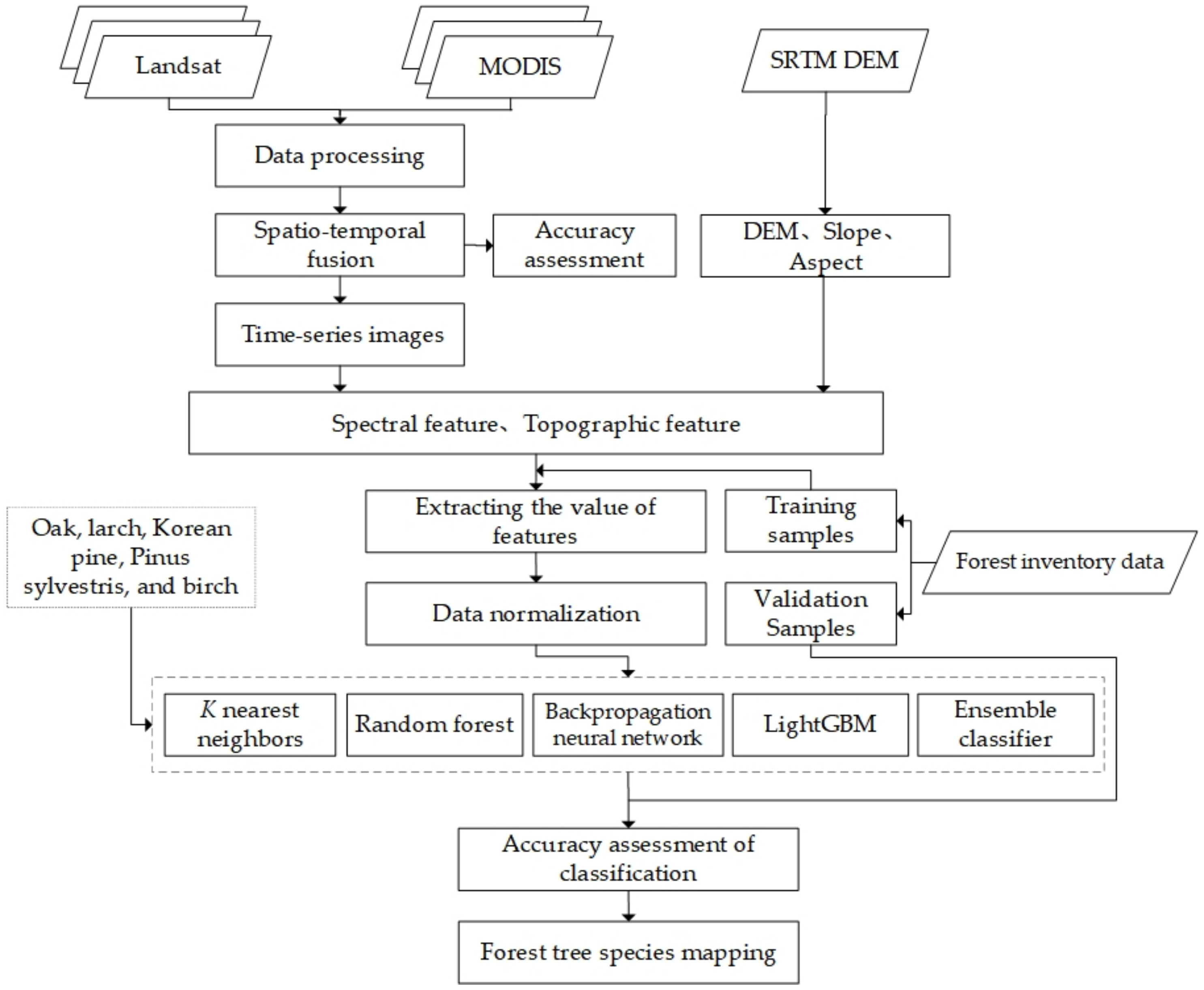
Our workflow includes (1) data preprocessing, (2) comparison and selection of spatiotemporal fusion methods, (3) generation of high-resolution time series images, (4) tree species classification based on various feature combinations and different classifiers, (5) classification accuracy assessment, and (6) tree species distribution mapping (Figure 2).

3.1. Remote Sensing Data and Preprocessing

The spatial resolution of the Landsat data is 30 m. However, the 16-day revisit cycle of Landsat has long limited its use for the study of global biophysical processes. MODIS involves daily data collection, so the probability of collecting cloud-free images is many times higher in MODIS compared to Landsat. However, the spatial resolution of MOIDS data at 500 m is not sufficient for mapping of tree species. Therefore, MODIS data were used to improve the temporal resolution of the available Landsat data for our study.
The only three cloud-free Landsat 8 OLI images in 2016 from different dates and the MCD43A4 product from MODIS on the same day were applied to select the best spatiotemporal fusion algorithm [45,46]. Each Landsat image consists of two adjacent paths (paths/rows: 116/30, 116/31). The image pair on May 19 was defined as the reference images of spatiotemporal fusion algorithms. The other two image pairs were used to assess the accuracy of different fusion algorithms. Figure 3 shows the MCD43A4 images of the base date (May 19) and two predicted dates (May 28 and October 19). The time series consisting of 28 images from March 21 to October 28 in the MCD43A4 product was input into the optimal spatiotemporal fusion algorithm to generate fine-pixel-resolution dense time series with 8-day intervals. The imaging time range of these images covers the whole growth period of various tree species. Table 1 lists the imaging date and spatiotemporal spectral information of all images. In addition, the Shuttle Radar Topography Mission (SRTM) V3 product provided by NASA JPL was selected to extract topographic information [47].
The MODIS and Landsat 8 images were acquired through the Google Earth Engine platform [48]. MODIS data preprocessing steps are as follows: (1) application of a forest mask to extract forest pixels, (2) filling in of missing values in the MCD43A4 images with image values from the same date in adjacent years [49,50], and (3) resampling of MODIS images to 30 m resolution using bicubic interpolation in ArcGIS 10.8. The USGS Landsat 8 Tier 1 dataset on the GEE platform was calibrated to surface reflectance after atmospheric and radiometric correction. Images taken on the same day were seamlessly mosaiced using ENVI 5.3 software and clipped to the forest area. The spatial reference for all data was unified to the WGS84 coordinate system.

3.2. Field Data

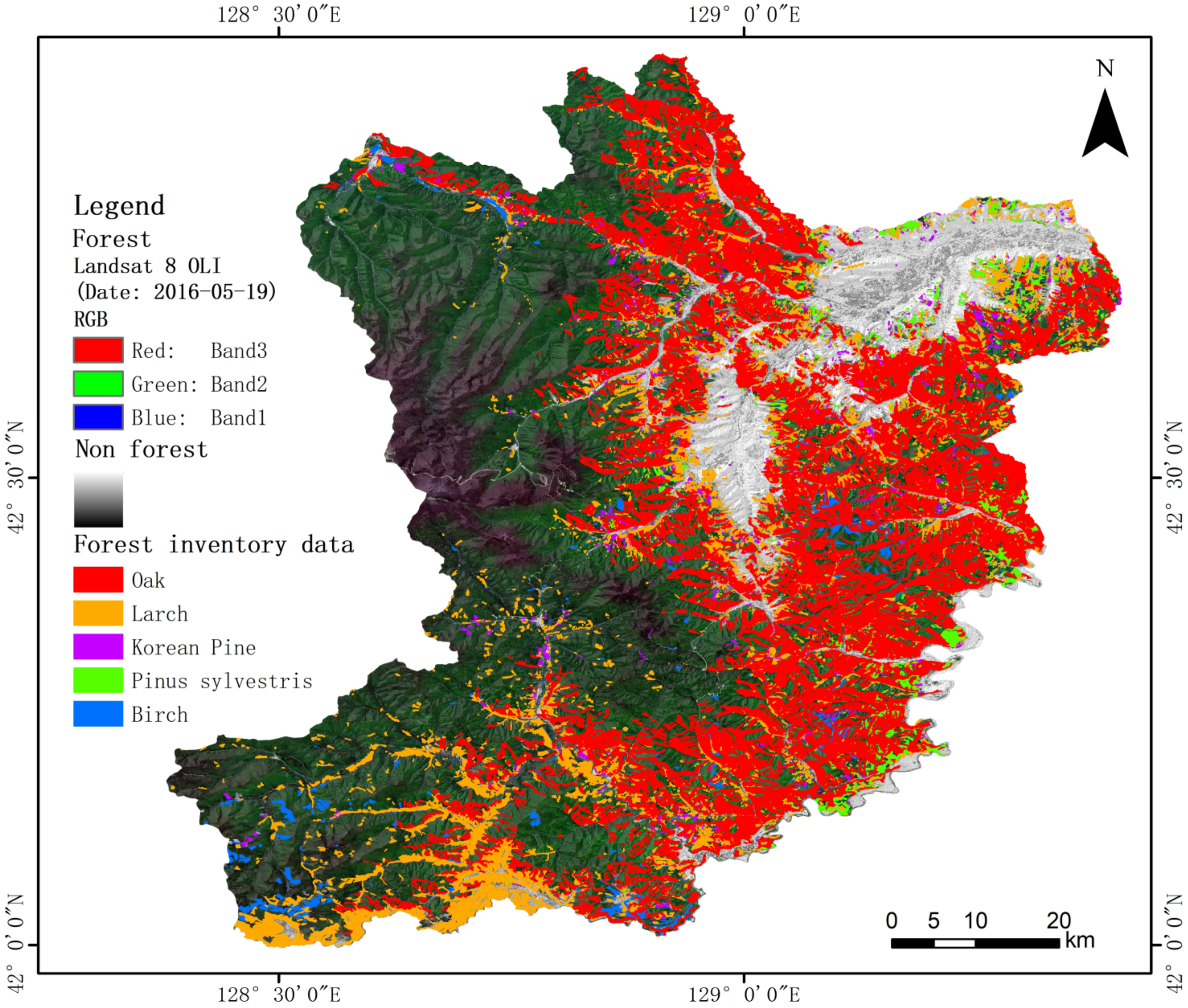
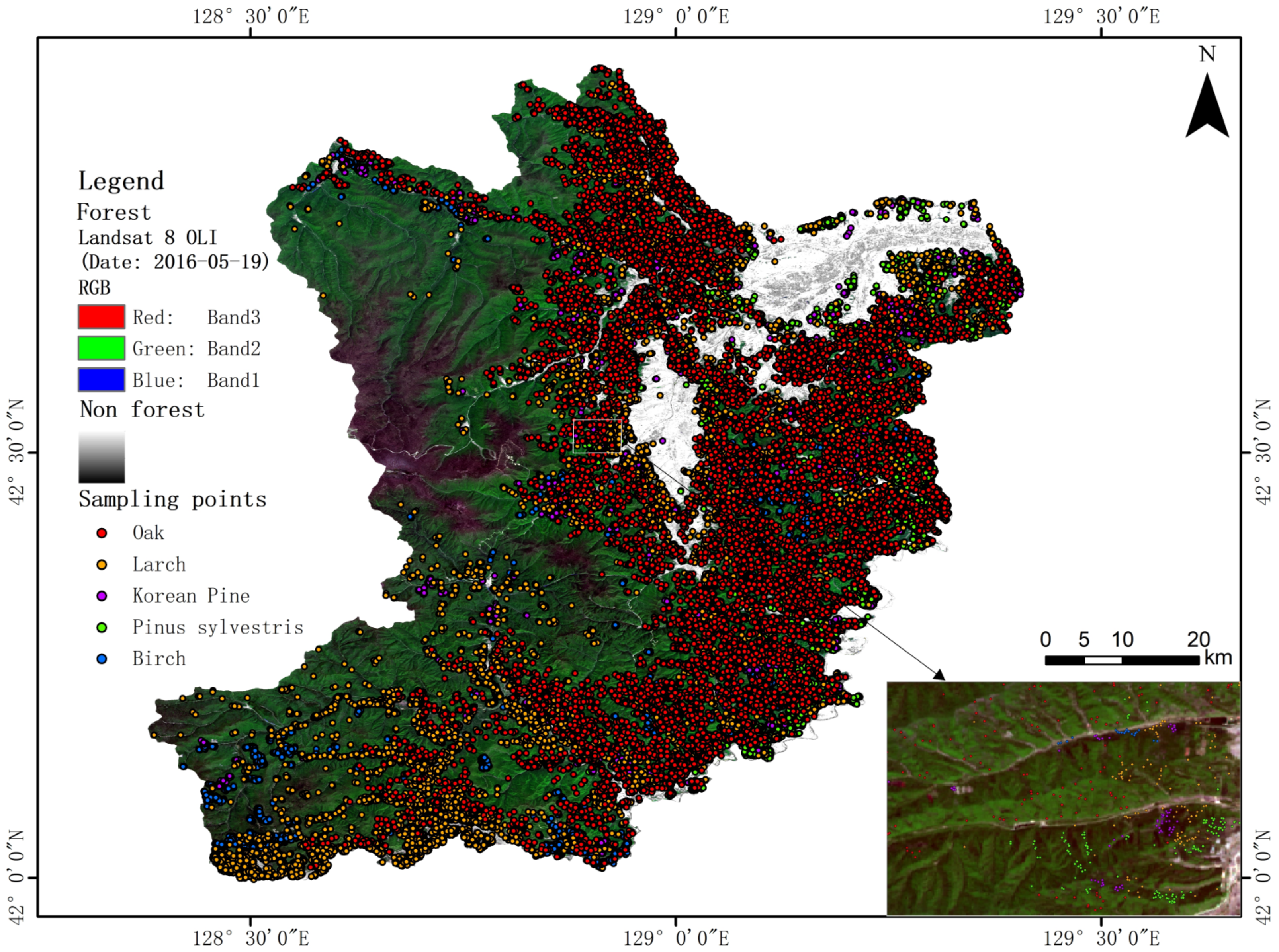
The reference data of land cover types and dominant tree species were derived based on the forest inventory data of Jilin Province for 2016 (Figure 4). In GIS, the data divide the study area into polygons representing separate, homogeneous stands. The training and validation samples were generated according to these data. The feature data of forests and five dominant tree species, i.e., oak, larch, Korean pine, Pinus sylvestris, and birch, were extracted separately, and small polygons with an area of less than 0.01 hm2 were removed. A 30 m inward buffer was applied to each polygon to minimize edge effects between patches of different tree species [51]. The sample points of each tree species were randomly sampled in the polygons (Figure 5). The minimum distance between adjacent sampling points was required to be greater than 30 m. Table 2 lists the number of samples for each tree species. Each category of sample points was randomly divided into a training set and a validation set in a ratio of 8:2. The training and validation samples do not contain the same sample points. The above process was completed using ArcGIS 10.8 software.

3.3. Spatiotemporal Fusion

Three typical spatiotemporal fusion methods were selected, i.e., STARFM, STNLFFM, and FSDAF. These fusion algorithms need at least one pair of high-resolution and low-resolution images at base date t0 and a known low-spatial-resolution image at predicted date tk; these images are then fused to obtain a high-spatial-resolution image for date tk. The Landsat 8 image and the MODIS image of May 19 (base date) were applied to predict the fused images on May 28 and October 19 (predicted date). The Landsat 8 images of May 28 and October 19 were used to verify the accuracy. The algorithm with the highest accuracy was selected to generate dense time series with 8-day intervals.

3.3.1. STARFM

The STARFM algorithm performs the fusion process using Equation (1) for MODIS (M) and Landsat (L):
L x w 2 , y w 2 , t k = i , j = 1 N W i j × M x i , y j , t k + L x i , y j , t 0 M x i , y j , t 0
where w is the size of the moving window, N is the number of similar pixels filtered by the local moving window, L x w 2 , y w 2 , t k is the value of the central pixel of the moving window for the Landsat image at predicted date t k , and x w 2 , y w 2 is the central pixel within the moving window. The spatial weighting function ( W i j ) determines how much each neighboring pixel ( x i , y j ) in w contributes to the estimated reflectance of the central pixel. M x i , y j , t k is the MODIS reflectance at the window location ( x i , y j ) observed at predicted date t k , while L x i , y j , t 0 and M x i , y j , t 0 are the corresponding Landsat and MODIS pixel values, respectively, observed on the base date ( t 0 ) [23].

3.3.2. FSDAF

FSDAF is a multisource remote sensing spatiotemporal fusion algorithm that combines unmixing, spatial interpolation, and similar neighboring pixel smoothing to obtain robust fusion results. It can be used to obtain land surface information of gradual changes or sudden changes in land cover types in heterogeneous regions [25]. First, FSDAF estimates the temporal variation of Landsat pixels Δ F t p based on the unmixing of the entire image to generate a temporal prediction ( F 2 t p ). Secondly, using thin-plate spline interpolation to generate spatial prediction ( F 2 S P ), the residuals between the Landsat pixels and the MODIS pixels are considered in FSDAF as [52]:
R x , y = Δ C x , y 1 n i = 1 n F 2 t p x i , y i i = 1 n F 1 x i , y i
where R x , y is the residual in the MODIS pixel at a given location x , y , n is the number of Landsat pixels inside a MODIS pixel, and the Landsat pixel at location x i , y i is inside the MODIS pixel at location x , y . In a homogenous area, spatial prediction performs well, which is applied to calculate a new residual [52]:
R h 0 x , y = F 2 S P x , y F 2 t p x , y
A weighted function ( w h ) is used for a homogeneity index of residual compensation to integrate the two residuals (i.e., R h 0 and R ). The final prediction of FSDAF can be expressed as [52]:
F 2 ^ x , y = F 1 x , y + i = 1 n s W i Δ F t p x i , y i + n × R x i , y i × w h x i , y i
where W i is the weight of similar pixels, and F 2 ^ x , y is the predicted image.

3.3.3. STNLFFM

STNLFFM extends the STARFM fusion framework. Based on the basic assumption of scale invariance between the temporal relationship of low-resolution images and the temporal relationship of high-resolution images, it solves the linear temporal relationship between the known low-resolution images of the base date and the predicted date and maps it to the high-resolution image to generate fusion results. This process can be expressed by Equation (5):
F x , y , t p = k = 1 M i = 1 N W ( x i , y i , t k ) × a x i , y i , Δ t k × F x i , y i , t k + b x i , y i , Δ t k
where F x , y , t p is the predicted image of the target pixel x , y for the predicted date t p ; M is the number of base (reference) dates; N is the total number of similar pixels (of the same type as the target pixel) in the image; x i , y i is the position of the ith similar pixel; a x i , y i , Δ t k ,   b x i , y i , Δ t k are the linear fit coefficients of the MODIS similar pixel set between the reference moment t k and the predicted moment t p , which are calculated using the least squares method; and W x i , y i , t k is the weight of the ith similar pixel of the Landsat image for the reference date ( t k ).

3.4. Tree Species Classification

The spectral reflectance (6 bands) and topographic features (3 variables) of elevation, slope, and aspect constitute input features that are combined in sets of up to 171 depending on the experiment [53]. The time series consists of 28 fused images. Each image contains 6 spectral bands. These variables and the three topographic features comprise up to 171 variables.
Seven experiments were set up to explore the effects of multitemporal spectral and topographic features on tree species classification. The input feature of experiment 1 was the single-temporal image surface reflectance. Experiment 2 added topographic features based on Experiment 1. Because the time series contains 28 images, both Experiment 1 and Experiment 2 needed to be performed 28 times. The input features of Experiment 3, Experiment 4, and Experiment 5 were the spectral features of spring, summer, and autumn images, respectively. The rest of the experiments were classified based on all spectral features. In addition, three experiments using real observation Landsat data were designed as a baseline to compare with experiments using fused images. These three experiments used the only three cloud-free Landsat images from 2016, the seasonal composite images of spring, summer, and autumn from 2016; and the seasonal composite images of spring, summer, and autumn from 2015, 2016, and 2017. Each composite image was obtained by averaging all available imagery throughout the season. The feature combinations for each experiment are shown in Table 3. All experiments used the same training and testing sampling points.
Four supervised classification methods, i.e., KNN [31], RF [33], ANN [34], and LightGBM [34], were selected in this research. In addition, a new ensemble model based on the soft voting strategy was proposed. The soft voting rule of an ensemble model on decision problem x works as follows [41]:
D x = m a x i d x i = 1 L w i d x , i
where D x is the selected class number of hard voting on decision problem x, L is the number of voters (base classifiers), d x , i is the binary vector output (e.g., [0, …, 0, 1, 0, …, 0]) of the classifier on decision problem x, w i is the weight of the ith base classifier, and m a x i d x is the index for which the maximum value was obtained in the summation vector ( i = 1 L w i d x , i ). Multiple maximum values return the index of first occurrence.
In our ensemble model, the results of KNN, RF, ANN, and LightGBM are fused with the same weights. The deep forest algorithm proposed by Zhou et al. was used for comparison with our proposed ensemble model [54]. This algorithm is a deep ensemble model. Its core technology is cascade forest and multigranularity scanning. This method requires little parameter tuning and performs better than traditional machine learning methods on many datasets.
The abovementioned algorithms were implemented using the scikit-learn and LightGBM libraries in Python [55]. Bayesian optimization was used to tune the main parameters of each method [56]. Table 4 lists the main parameter settings for base classifiers.

3.5. Accuracy Assessment

Five metrics were chosen to assess the performance of the three spatiotemporal fusion algorithms, i.e., correlation coefficient (CC), root mean square error (RMSE), structural similarity index (SSIM), spectral angle (SAM), and global relative error (ERGAS) (Equations (7)–(11)) [57,58,59]. A total of 10,000 pixels were randomly selected, and the correlation coefficients (Equation (12)) between the predicted images (pixel values) and the actual Landsat 8 image in the red and near-infrared bands on the two predicted dates were calculated. Relevant studies have shown that the red band and the near-infrared band are most related to the chlorophyll content and water content of vegetation, respectively [55]. The Landsat image on the base date was compared to Landsat images on the two predicted dates as a control. The correlation coefficients between each band and their average were calculated.
CC F , G = 1 B b = 1 B c o v F b , G b σ F b σ G b
where F and G represent the fusion image and the real image, respectively; c o v (·) is the covariance; σ represents the standard deviation of the image; b is the band number; and B is the total number of bands.
RMSE F , G = 1 B b = 1 B F b G b 2 N 1 N 2
where N 1 and N 2 are the height and width of the image, respectively.
SSIM F , G = 1 B b = 1 B 2 μ F b μ G b + C 1 2 c o v F b , G b + C 2 μ F b 2 + μ G b 2 + C 1 σ F b 2 + σ G b 2 + C 2
where μ represents the mean value of a given band of the image.
SAM F , G = 1 N 1 N 2 i = 1 N 1 N 2 a r c c o s V F i T V G i V F i 2 · V G i 2
where V F i and V G i are the spectral vectors of the ith pixel of images F and G, respectively.
ERGAS = 100 h l 1 B b = 1 B R M S E b 2 μ G b 2
where h is the spatial resolution of the high-resolution image, and l is the spatial resolution of the low-resolution image.
r X , Y = C o v X , Y V a r X V a r Y
where X and Y are the pixel-value vectors of the fusion image and the real image, respectively; Cov(X,Y) is the covariance of X and Y; Var[X] is the variance of X; and Var[Y] is the variance of Y.
The overall accuracy of tree species classification was assessed using the overall accuracy (OA) and kappa coefficient (Equations (13) and (14)). The class-wise accuracies were evaluated by the producer accuracy (PA), user accuracy (UA), and F-value (Equations (15)–(17)) [60].
OA = T P + T N T P + T N + F P + F N
Kappa = P 0 P e 1 P e
PA = T P T P + F N
UA = T P T P + F P
F 1 = 2 × U A × P A U A + P A
where TP is true positive, representing the number of correct predictions for positive samples; TN is true negative, showing the number of correct predictions for negative samples; FP is false positive, indicating the number of incorrect predictions for positive samples; FN is false negative, denoting the number of incorrect predictions for negative samples; Po is the number of correctly predicted samples divided by the total number of samples; and Pe is equal to (a1 × b1 + a2 × b2 + … + am × bm)/n × n, where a1 to am represent the number of true samples for each tree species, and b1 to bm indicate the number of samples predicted for each tree species.

4. Results

4.1. Image Fusion and Evaluation

The STARFM, FSDAF, and STNLFFM were applied to generate the fused images of May 28 and October 19. Figure 6 shows a comparison of the Landsat image of the base date and the Landsat images of the two predicted dates. Table 5 shows the correlation coefficients of each band and their mean values between the Landsat images of the base date and the predicted date. Compared with the Landsat image of October 19, the reflectance of the Landsat image on May 28 was closer to the Landsat image of the base date. The correlation coefficient of each band on May 28 was also higher, which was an average of 0.12 higher than that on October 19. The Landsat images between the two prediction dates and the base date were significantly correlated, and the correlation coefficients were both greater than 0.8. MODIS pixels, which is equivalent to aggregating multiple Landsat pixels at the same location. This temporal correlation also exists on MODIS images. Therefore, high-quality Landsat-like images can be generated through spatiotemporal fusion technology based on MODIS.
Figure 7 shows a typical region of these fused images. Table 6 shows the metrics of different methods. It can be seen that the fusion accuracy of the two dates varies greatly. The fusion results of different algorithms on May 28 are very similar and satisfactory. The high accuracy metrics indicate very little difference between fused and reference images. On October 19, the performance of the three algorithms was significantly worse than that on May 28. The levels of several metrics were also significantly lower but still acceptable. Among the three algorithms, STNLFFM achieved the highest accuracy. The STARFM model performed slightly worse than STNLFFM. FSDAF is the most unsatisfactory algorithm because the fusion results were severely blurred, and a considerable amount of spatial information was lost.
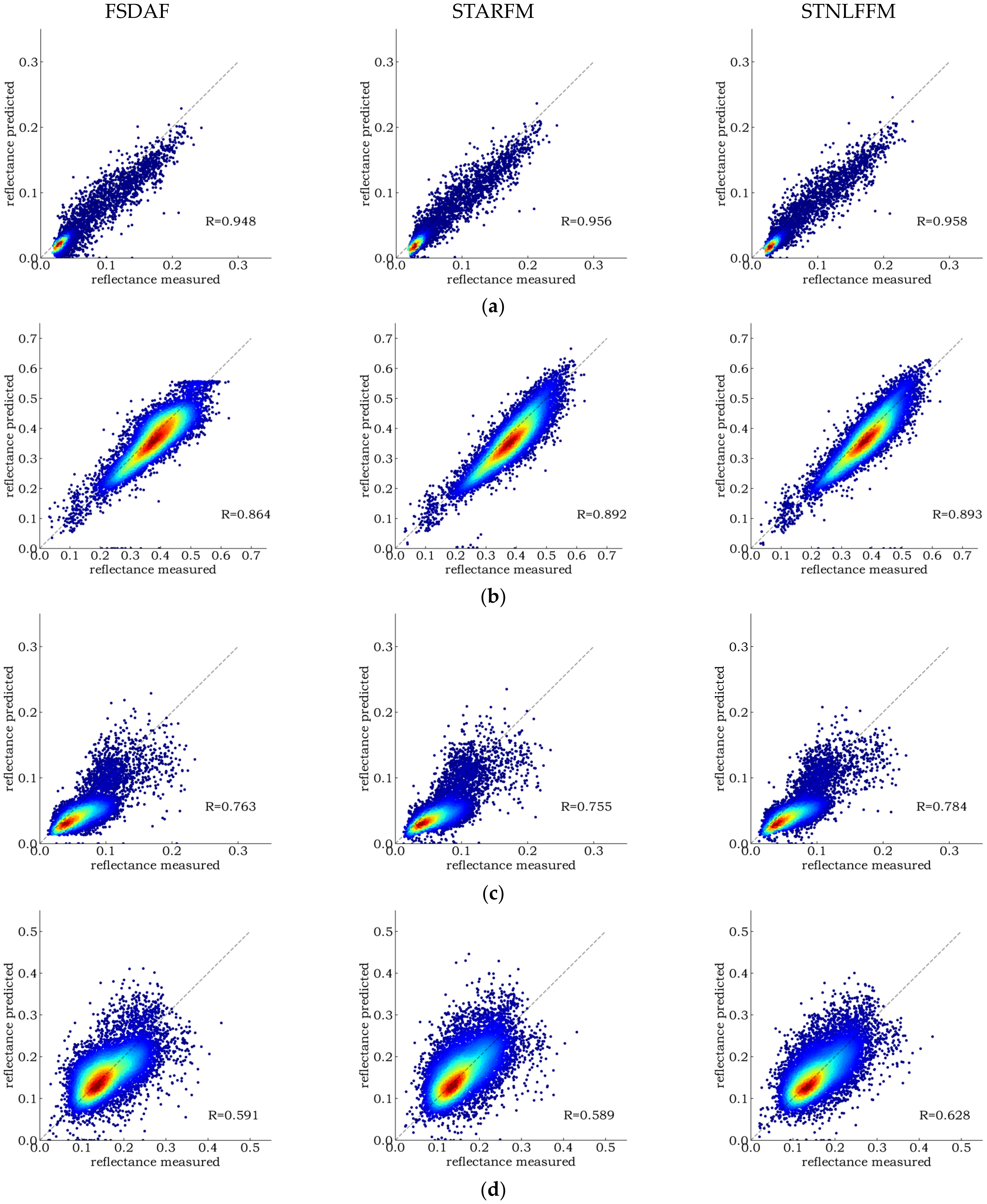
The scatter plots in Figure 8 show the correlation of the red and near-infrared bands between the fused and reference images. The STNFLLM correlation coefficient is always the highest, which indicates that the fusion results correlate more with the actual observations. The average correlation coefficient of STARFM is close to that of STNLFFM and higher than that of FSDAF. In conclusion, STNLFFM performed best in both qualitative and quantitative evaluations. Therefore, the STNLFFM algorithm was selected to generate dense time series images for tree species classification.

4.2. Classification and Mapping of Tree Species

4.2.1. The Overall Accuracy of Five Tree Species

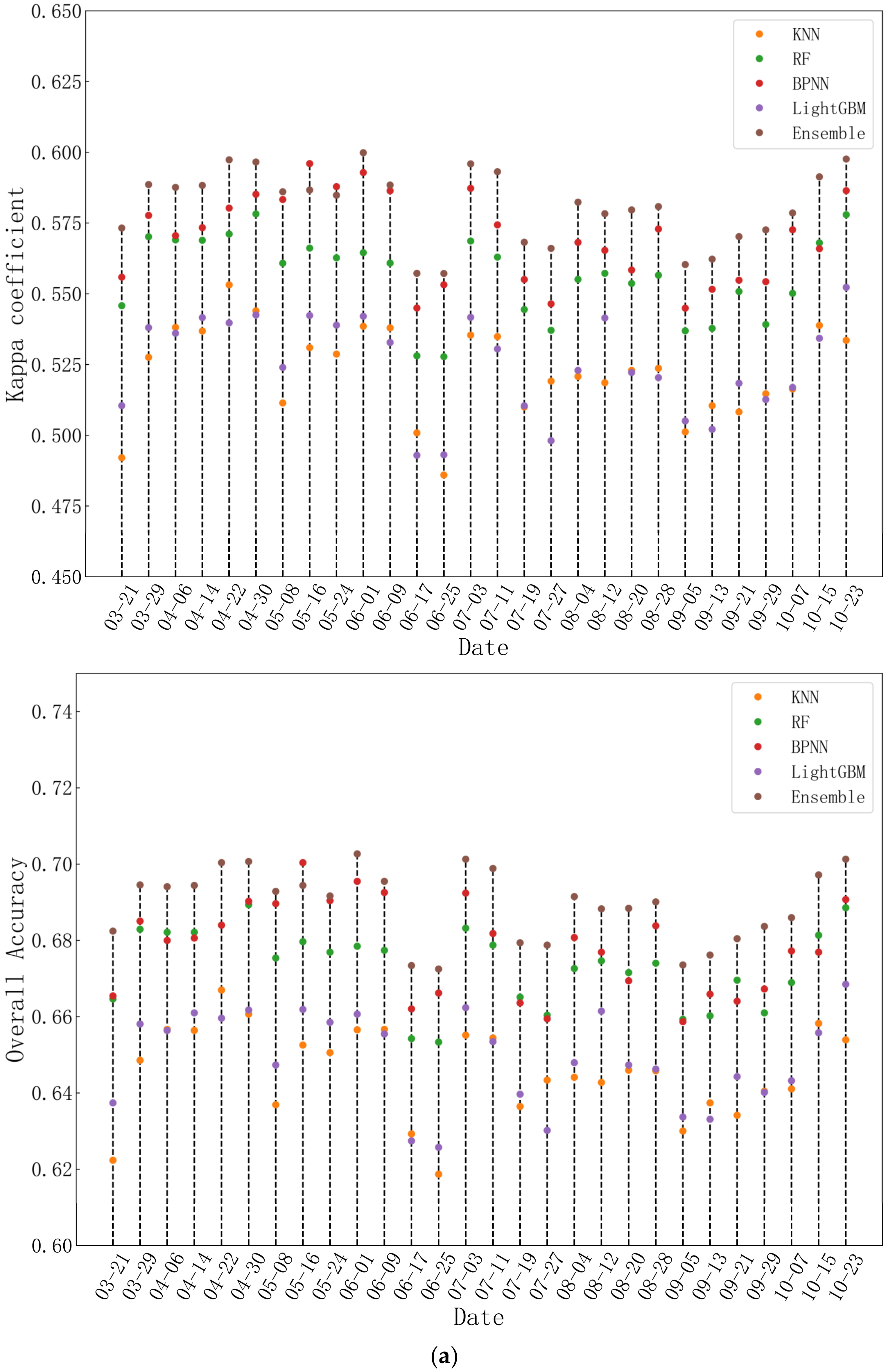
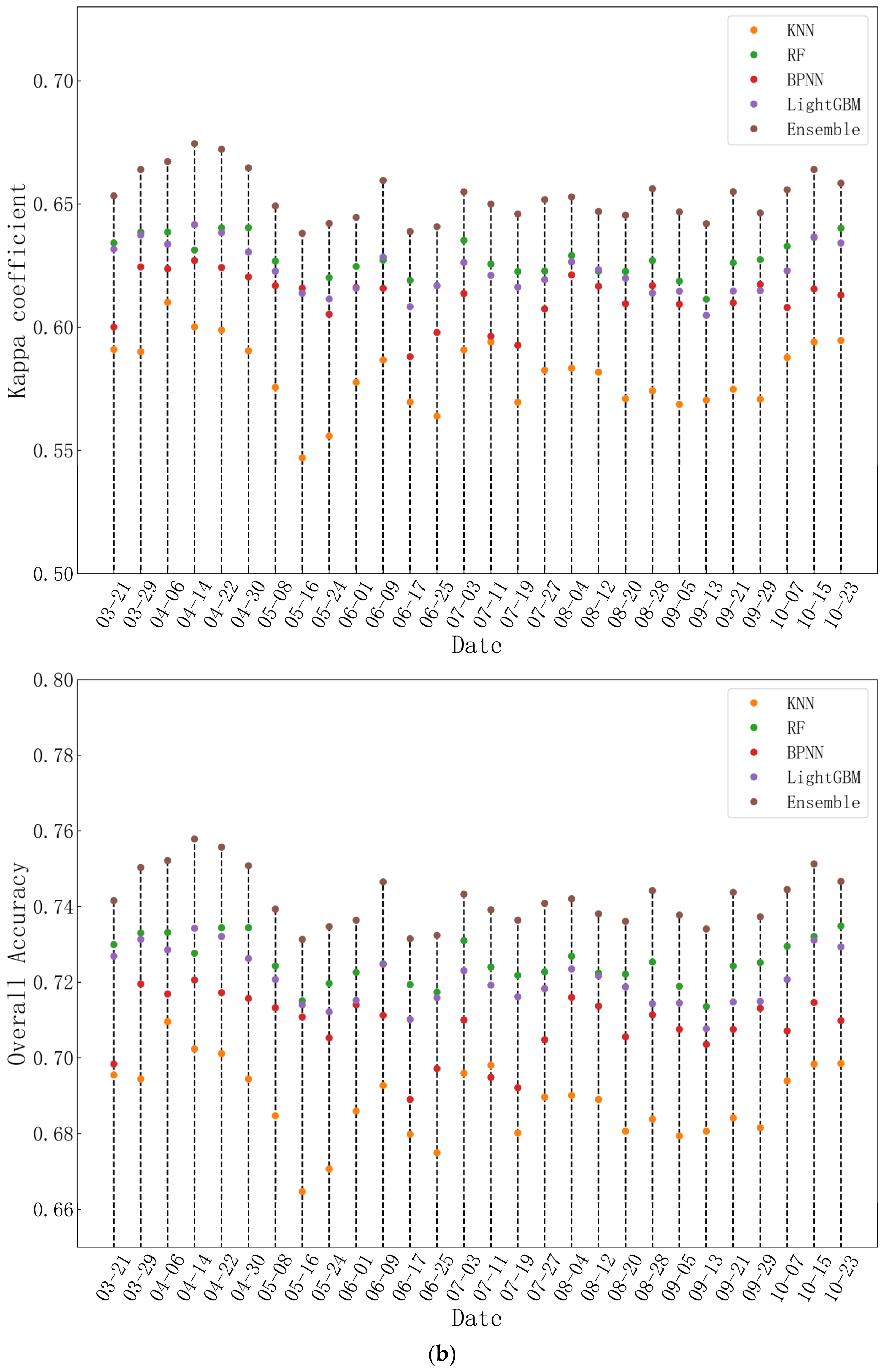
Four existing machine learning algorithms and our proposed ensemble algorithm were used to classify tree species in ten experiments. Lollipop plots were generated to display the accuracy for different dates in Experiment 1 and Experiment 2 (Figure 9). Table 7 shows the kappa coefficients and overall accuracy for all experiments. The accuracy of Experiment 1 and Experiment 2 is the mean value of the whole experiment.
Figure 9 shows that the classification accuracy is not satisfactory based only on a single image. The kappa coefficient is only around 0.55, and the overall accuracy is approximately 65%. The introduction of topographic features in Experiment 2 significantly improved the classification accuracy by approximately 6% overall, with a kappa coefficient improvement of approximately 0.07. Table 7 shows that multitemporal images can significantly enhance classification precision compared with single-temporal classification. Satisfactory accuracy can be achieved using images from only one season. When using the ensemble classifier based on images of different seasons, the kappa coefficients were all higher than 0.75, and the overall accuracy was higher than 0.8. The classification based on spring images had the highest accuracy among the three seasons, with 82.41% OA and a 0.765 kappa coefficient. Adding topographic features to time series data improved classification accuracy, but the effect was not as pronounced as adding it to single-phase images. Compared with using only three Landsat images and seasonal composite images from one year and three years, the overall accuracy classification using the full time series, topographic variables, and the ensemble classifier was improved by 11.4%, 12.48%, and 4.87%, respectively. Therefore, the complete fused time series with topographic features as auxiliary variables constitutes the optimal feature combination.
The performance of the evaluated classifiers differed significantly. In Experiment 1, ANN and RF significantly outperformed KNN and LightGBM. After adding topographic features, the model with the highest average overall accuracy was RF, followed by LightGBM, ANN, and KNN. In multitemporal classification, ANN and LightGBM achieved significantly higher classification accuracy than KNN and RF. However, the ensemble classifier achieved the highest accuracy in almost all experiments. Compared to the best base classifier, the most significant improvements in overall accuracy and kappa coefficients were around 3.4% and 0.047, respectively. When classifying based on the optimal feature combination in Experiment 7, compared with KNN, RF, ANN, and LightGBM, the classification accuracy of the ensemble classifier was improved by 4.89%, 4.07%, 1.42%, and 1.56%, respectively. Therefore, the ensemble classifier was ultimately selected for tree species mapping.

4.2.2. The Class-Wise Accuracies of Five Tree Species

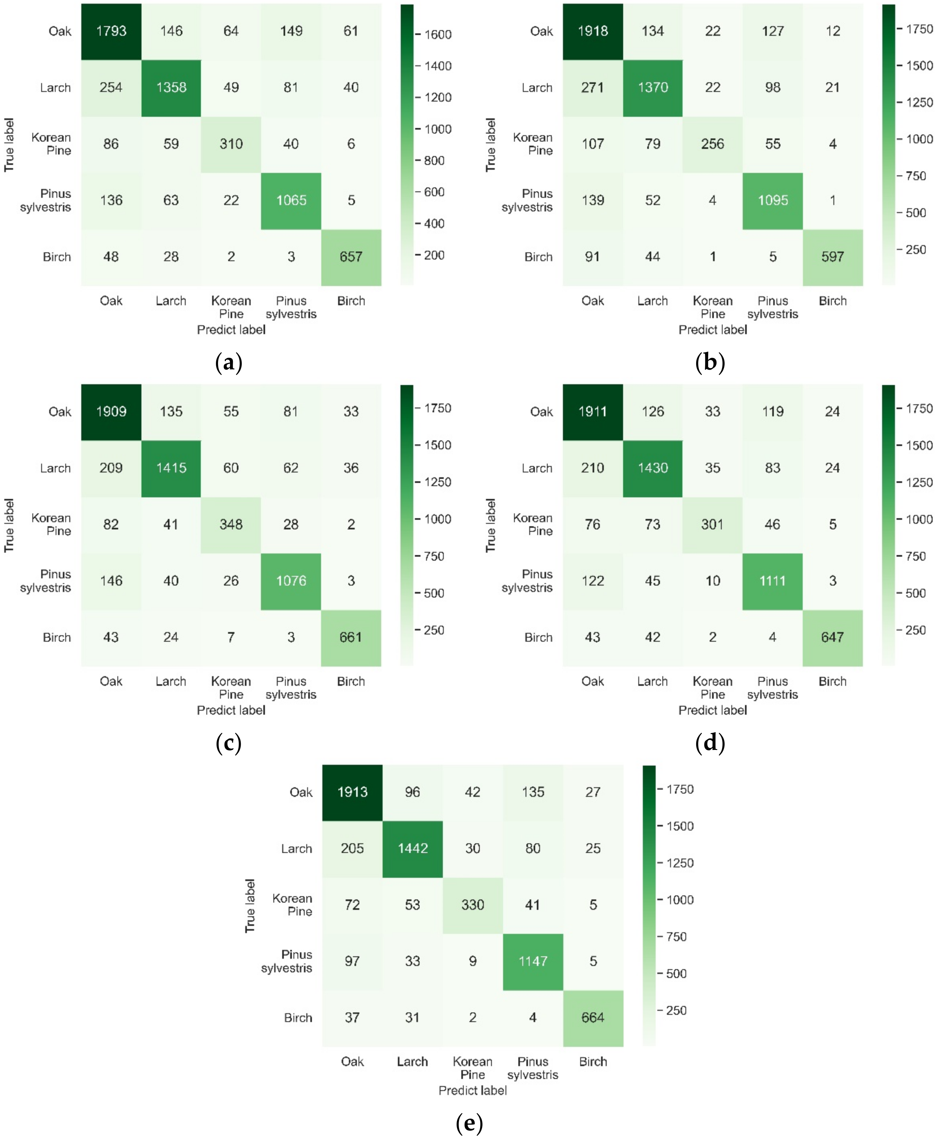
The user accuracy, producer accuracy, and F-value of each classifier in Experiment 7 are reported in Table 8. As a control, the mean user accuracy, producer accuracy, and F-value of the other nine experiments are reported in Table 9. The confusion matrix for each classifier is shown in Figure 10. The F-value was chosen to measure the classification accuracy of each category. The ensemble method achieved the highest accuracy in all classes of tree species. Except for Korean pine, the classification accuracy was satisfactory, and the F-value was above 80%. Birch had the highest classification accuracy at 90.71%. In contrast, Korean pine had the lowest classification accuracy, with an F-value of 72.21%. However, the ensemble classifier exhibited the most significant improvement in classification accuracy of this category, with the F-value improved by approximately 2.5% compared with ANN.

4.2.3. Comparison with Other Ensemble Models

Table 10 shows the classification accuracy of the deep forest algorithm and our proposed ensemble method with the optimal feature combination (Experiment 7). The overall accuracy of our ensemble model was about 2% higher than that of the deep forest model, which indicates that our proposed model is more advanced.

4.2.4. Tree Species Mapping

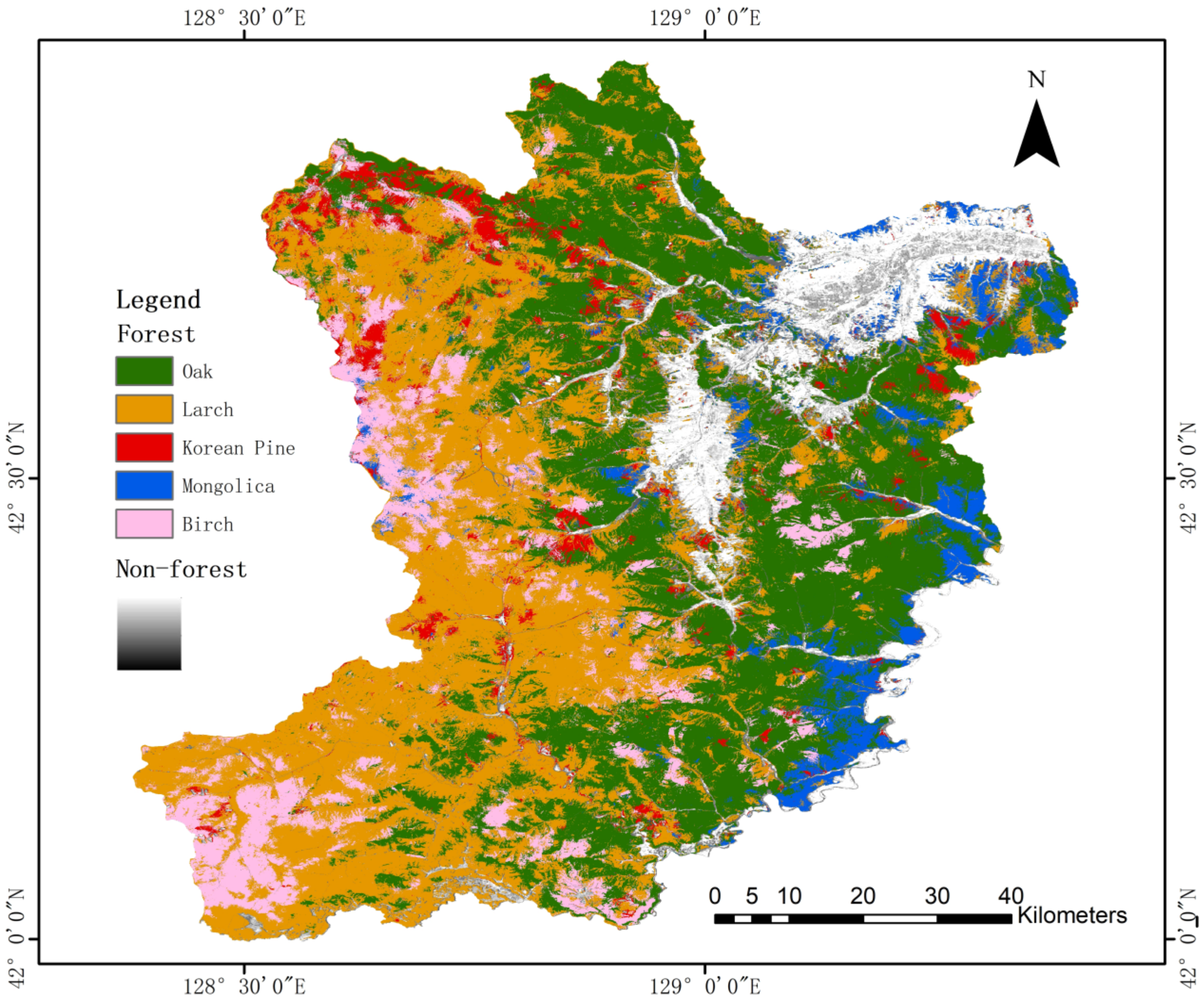
A tree species distribution map of the study area (Figure 11) was produced using the ensemble classifier based on spectral and topographic features. The most common species were oak (39.15%) and larch (39.87%), whereas the other three species were relatively less distributed, with area proportions of 4.65% (Korean Pine), 5.40% (Pinus sylvestris), and 10.93% (Birch).

5. Discussion

5.1. Error Sources in Spatiotemporal Fusion Algorithms

The three spatiotemporal fusion methods are mathematically different. By assuming a linear relationship between fine and coarse images or between coarse prediction and base date images, STARFM uses a linear regression model to describe this linear relationship, followed by prediction through the application of the linear regression model to the coarse image on the prediction date or the fine image on the base date. However, the performance of STARFM for reflectance change areas and heterogeneous landscapes is not satisfactory [61]. The flexible spatiotemporal data fusion (FSDAF) model is a method involving the use of one pair of fine- and coarse-resolution images and one coarse-resolution image acquired on the prediction date. This method integrates unmixing-based methods, spatial interpolation, and STARFM into one framework. However, this method is computationally expensive, and the prediction accuracy greatly depends on the extent of land cover changes between the two dates of the input images [62]. In STNLFFM, the coefficients of the linear equation of a given pair of coarse-spatial-resolution pixels can be acquired using the least squares method based on the neighboring pixels and the given pixels themselves. Then, the coefficients can be used for the observed fine-spatial-resolution image to acquire a prediction. To decrease the effects of heterogeneous landscapes, STNLFFM uses neighboring spectrally similar pixels to make a more accurate prediction [63]. The accuracy of the three fusion algorithms is similar and acceptable. STNLFFM performs best because it pays more attention to changes in the reflectance of multitemporal images [64]. However, it is necessary to point out that the fusion precision of all methods on October 19 was lower than that on May 28 because the time interval between the prediction and reference dates was longer. The difference in phenology was more significant, leading to a decrease in fusion accuracy [21]. In cases in which the reference and prediction dates are closer and the correlation between the images is strong, the prediction results are generally more reliable [65]. Another limitation of the three algorithms described above is that these methods only use information from images obtained on the two individual dates and ignore the temporal information of time series with different resolutions. The use of additional images can help to improve fusion results [66].

5.2. The Influence of Different Features on Classification Accuracy

In different feature combinations, the classification accuracy increases continuously with the number of images because multitemporal or time series data contain phonological and tree species growth information, and growth characteristics differ depending on the tree species [13,51,67]. Tree species are difficult to classify in a single temporal image, but time series growth information benefits tree species discrimination [68]. Among topographic features, elevation is highly correlated with tree species distribution. Larch and birch trees are mainly distributed in high-altitude regions. In contrast, the other three tree species are distributed primarily in flat areas. Therefore, when the input data are only a single temporal image, topographic features can complement single-temporal spectral information and significantly improve classification accuracy. However, when the input features contain enough temporal-phase spectral features, topographic features can only slightly improve the accuracy because the classification is mainly based on spectral features [69].

5.3. The Advantages and Limitations of Ensemble Classifiers

The proposed ensemble classifier combining KNN, RF, ANN, and LightGBM consistently achieved the best accuracy. By introducing the advanced classification methods of ANN and LightGBM, the ensemble model we proposed not only performed well on low-dimensional data but also on high-dimensional data such as time series. Compared with other studies, our reported classification accuracy is similar [70]. The classification accuracy of Korean pine was the least satisfactory, possibly owing to the small number of samples and the uncertainty of the reference data. The confusion matrix shows that the ensemble model reduced the occurrence of misclassification and underclassification. Our results reflect the effectiveness and generalizability of ensemble learning in tree species classification. However, compared to ANN, the number of correctly classified pixels of Korean pine was reduced in the ensemble method because KNN, RF, and LightGBM have lower classification accuracies for Korean pine. These classifiers did not help the classification of Korean pine in the ensemble model but reduced its classification accuracy. The soft voting strategy is simple and easy to implement, but there are still some limitations in selecting its base classifiers. First, the classification results between base models should not differ too much. When a base model works poorly relative to other models, the results are likely to become noise and affect the ensemble effect, and there should be less homogeneity among the base models [71].

5.4. Comparison with Other Studies

We compared our results with those reported in similar studies. In terms of spatiotemporal fusion, the fusion accuracies were close to those of the associated developers [23,24,25]. Cheng et al. showed that STNLFFM always outperforms STARFM. The correlation coefficients between the fusion image and the real Landsat image of STNLFFM in the two test areas were all higher than 0.9 [24]. In a study by Li et al., FSDAF predicted blurred image texture information with unclear edges [72]. These results are consistent with our findings. In terms of tree species classification, Wang et al. fused GF-1, Landsat 8, and MODIS NDVI data to obtain enough spatial and temporal resolution for six forest types distinguished in Duchang County by utilizing the STNLFFM model and support vector machines [64], achieving an overall accuracy of 82%, which is slightly lower than that reported in our study. The tree species classification system proposed in a study by Joongbin Lim et al. is similar to ours [70]. They developed a model to classify the five dominant tree species in North Korea (Korean red pine, Korean pine, Japanese larch, needle fir, and oak) using Sentinel-2 data and machine learning techniques. In the Gwangneung Forest area, the proposed model achieved an overall accuracy of 83%, which is at the same level as our results (84.32%). However, the spatial resolution of the Sentinel-2 images they used was 10 m. This is higher than the 30 m of the Landsat-like time series we used in the present study. The above comparisons show the reliability and advances achieved in our research.

6. Conclusions

Owing to the poor availability of remote sensing data, tree species classification in cloudy mountain areas remains a challenge. In this research, we improved tree species mapping in cloudy mountainous regions from the perspectives of remote sensing data, classification features, and classification algorithms. Three spatiotemporal fusion methods, i.e., FSDAF, STARFM, and STNLFFM, were compared. The best-performing STNLFFM algorithm was applied to generate a dense time series with 8-day intervals. In addition to the spectral features of the fused time series, topographic features were also added to the classification procedure. KNN, RF, ANN, LightGBM, and our proposed ensemble classifier were selected for tree species classification. The results show that the fused time series improved the classification accuracy by approximately 20% compared with the single-phase images. The ensemble classifier consistently achieved the highest accuracy, with a maximum improvement of approximately 3.4% compared to the best base classifier. The final classification accuracy reached 84.32%. In conclusion, it is necessary to use spatiotemporal fusion to generate dense time series to alleviate the problem of poor image availability in cloudy mountainous areas. Topographic features also help to enhance the classification precision of tree species in mountainous areas. The ensemble classifier, which combines the results of multiple classifiers, is suitable for classification based on time series images and can effectively reduce the misclassification of pixels. This study illustrates a tree species classification method integrating temporal and spatial information from remote sensing data with differing resolution in areas with poor data availability and represents a valuable reference for improved tree species mapping.

Author Contributions

All of authors contributed to the study. L.C. designed and completed the whole experiment and wrote the paper. S.C., X.Z., Y.M., X.X. and B.Z. revised the paper and provided valuable advice for the experiments. All authors have read and agreed to the published version of the manuscript.

Funding

This research was funded and supported by the National Key Research and Development Program of China (No. 2020YFA0714103), capital construction funds (innovative capacity building) within the provincial budget in 2021 (No.2021C045-8), the Jilin Province Science and Technology Development Plan Project (No.20210201138GX), and the Science and technology project in Chaoyang District, Changchun City (Chaoyang Science and Technology Co-202101).

Informed Consent Statement

Not applicable.

Data Availability Statement

Not applicable.

Conflicts of Interest

The authors declare no conflict of interest.

References

  1. Portillo-Quintero, C.; Sanchez-Azofeifa, A.; Calvo-Alvarado, J.; Quesada, M.; do Espirito Santo, M.M. The role of tropical dry forests for biodiversity, carbon and water conservation in the neotropics: Lessons learned and opportunities for its sustainable management. Reg. Environ. Chang. 2015, 15, 1039–1049. [Google Scholar] [CrossRef]
  2. Watson, J.E.; Evans, T.; Venter, O.; Williams, B.; Tulloch, A.; Stewart, C.; Thompson, I.; Ray, J.C.; Murray, K.; Salazar, A. The exceptional value of intact forest ecosystems. Nat. Ecol. Evol. 2018, 2, 599–610. [Google Scholar] [CrossRef] [PubMed]
  3. Führer, E. Forest functions, ecosystem stability and management. For. Ecol. Manag. 2000, 132, 29–38. [Google Scholar] [CrossRef]
  4. Chiarucci, A.; Piovesan, G. Need for a global map of forest naturalness for a sustainable future. Conserv. Biol. 2020, 34, 368–372. [Google Scholar] [CrossRef] [PubMed]
  5. McRoberts, R.E.; Tomppo, E.O. Remote sensing support for national forest inventories. Remote Sens. Environ. 2007, 110, 412–419. [Google Scholar] [CrossRef]
  6. Hemmerling, J.; Pflugmacher, D.; Hostert, P. Mapping temperate forest tree species using dense Sentinel-2 time series. Remote Sens. Environ. 2021, 267, 112743. [Google Scholar] [CrossRef]
  7. Lim, J.; Kim, K.-M.; Jin, R. Tree species classification using hyperion and sentinel-2 data with machine learning in South Korea and China. ISPRS Int. J. Geo-Inf. 2019, 8, 150. [Google Scholar] [CrossRef] [Green Version]
  8. Harikumar, A.; Paris, C.; Bovolo, F.; Bruzzone, L. A crown quantization-based approach to tree-species classification using high-density airborne laser scanning data. IEEE Trans. Geosci. Remote Sens. 2020, 59, 4444–4453. [Google Scholar] [CrossRef]
  9. Li, Z.; Zhang, Q.-Y.; Qiu, X.-C.; Peng, D.-L. Temporal stage and method selection of tree species classification based on GF-2 remote sensing image. Ying Yong Sheng Tai Xue Bao J. Appl. Ecol. 2019, 30, 4059–4070. [Google Scholar]
  10. Grabska, E.; Hostert, P.; Pflugmacher, D.; Ostapowicz, K. Forest stand species mapping using the Sentinel-2 time series. Remote Sens. 2019, 11, 1197. [Google Scholar] [CrossRef] [Green Version]
  11. Bjerreskov, K.S.; Nord-Larsen, T.; Fensholt, R. Classification of nemoral forests with fusion of multi-temporal sentinel-1 and 2 data. Remote Sens. 2021, 13, 950. [Google Scholar] [CrossRef]
  12. Grybas, H.; Congalton, R.G. A comparison of multi-temporal RGB and multispectral UAS imagery for tree species classification in heterogeneous New Hampshire Forests. Remote Sens. 2021, 13, 2631. [Google Scholar] [CrossRef]
  13. Persson, M.; Lindberg, E.; Reese, H. Tree species classification with multi-temporal Sentinel-2 data. Remote Sens. 2018, 10, 1794. [Google Scholar] [CrossRef] [Green Version]
  14. Liu, H. Classification of urban tree species using multi-features derived from four-season RedEdge-MX data. Comput. Electron. Agric. 2022, 194, 106794. [Google Scholar] [CrossRef]
  15. Sheeren, D.; Fauvel, M.; Josipović, V.; Lopes, M.; Planque, C.; Willm, J.; Dejoux, J.-F. Tree species classification in temperate forests using Formosat-2 satellite image time series. Remote Sens. 2016, 8, 734. [Google Scholar] [CrossRef] [Green Version]
  16. Wan, H.; Tang, Y.; Jing, L.; Li, H.; Qiu, F.; Wu, W. Tree species classification of forest stands using multisource remote sensing data. Remote Sens. 2021, 13, 144. [Google Scholar] [CrossRef]
  17. Xu, K.; Zhang, Z.; Yu, W.; Zhao, P.; Yue, J.; Deng, Y.; Geng, J. How spatial resolution affects forest phenology and tree-species classification based on satellite and up-scaled time-series images. Remote Sens. 2021, 13, 2716. [Google Scholar] [CrossRef]
  18. Xu, K.; Tian, Q.; Zhang, Z.; Yue, J.; Chang, C.-T. Tree species (genera) identification with GF-1 time-series in a forested landscape, Northeast China. Remote Sens. 2020, 12, 1554. [Google Scholar] [CrossRef]
  19. Belgiu, M.; Stein, A. Spatiotemporal image fusion in remote sensing. Remote Sens. 2019, 11, 818. [Google Scholar] [CrossRef] [Green Version]
  20. Gao, F.; Hilker, T.; Zhu, X.; Anderson, M.; Masek, J.; Wang, P.; Yang, Y. Fusing Landsat and MODIS data for vegetation monitoring. IEEE Geosci. Remote Sens. Mag. 2015, 3, 47–60. [Google Scholar] [CrossRef]
  21. Chen, B.; Huang, B.; Xu, B. Comparison of spatiotemporal fusion models: A review. Remote Sens. 2015, 7, 1798–1835. [Google Scholar] [CrossRef]
  22. Zhu, X.; Cai, F.; Tian, J.; Williams, T.K.-A. Spatiotemporal fusion of multisource remote sensing data: Literature survey, taxonomy, principles, applications, and future directions. Remote Sens. 2018, 10, 527. [Google Scholar] [CrossRef] [Green Version]
  23. Gao, F.; Masek, J.; Schwaller, M.; Hall, F. On the blending of the Landsat and MODIS surface reflectance: Predicting daily Landsat surface reflectance. IEEE Trans. Geosci. Remote Sens. 2006, 44, 2207–2218. [Google Scholar]
  24. Cheng, Q.; Liu, H.; Shen, H.; Wu, P.; Zhang, L. A spatial and temporal nonlocal filter-based data fusion method. IEEE Trans. Geosci. Remote Sens. 2017, 55, 4476–4488. [Google Scholar] [CrossRef] [Green Version]
  25. Zhu, X.; Helmer, E.H.; Gao, F.; Liu, D.; Chen, J.; Lefsky, M.A. A flexible spatiotemporal method for fusing satellite images with different resolutions. Remote Sens. Environ. 2016, 172, 165–177. [Google Scholar] [CrossRef]
  26. Gao, F.; Anderson, M.C.; Zhang, X.; Yang, Z.; Alfieri, J.G.; Kustas, W.P.; Mueller, R.; Johnson, D.M.; Prueger, J.H. Toward mapping crop progress at field scales through fusion of Landsat and MODIS imagery. Remote Sens. Environ. 2017, 188, 9–25. [Google Scholar] [CrossRef] [Green Version]
  27. Zhang, B.; Zhang, L.; Xie, D.; Yin, X.; Liu, C.; Liu, G. Application of Synthetic NDVI Time Series Blended from Landsat and MODIS Data for Grassland Biomass Estimation. Remote Sens. 2015, 8, 10. [Google Scholar] [CrossRef] [Green Version]
  28. Jia, K.; Liang, S.; Wei, X.; Yao, Y.; Su, Y.; Jiang, B.; Wang, X. Land Cover Classification of Landsat Data with Phenological Features Extracted from Time Series MODIS NDVI Data. Remote Sens. 2014, 6, 11518–11532. [Google Scholar] [CrossRef] [Green Version]
  29. Chaudhuri, P.; Ghosh, A.K.; Oja, H. Classification based on hybridization of parametric and nonparametric classifiers. IEEE Trans. Pattern Anal. Mach. Intell. 2008, 31, 1153–1164. [Google Scholar] [CrossRef]
  30. Axelsson, A.; Lindberg, E.; Reese, H.; Olsson, H. Tree species classification using Sentinel-2 imagery and Bayesian inference. Int. J. Appl. Earth Obs. Geoinf. 2021, 100, 102318. [Google Scholar] [CrossRef]
  31. Zhang, M.-L.; Zhou, Z.-H. ML-KNN: A lazy learning approach to multi-label learning. Pattern Recognit. 2007, 40, 2038–2048. [Google Scholar] [CrossRef] [Green Version]
  32. Noble, W.S. What is a support vector machine? Nat. Biotechnol. 2006, 24, 1565–1567. [Google Scholar] [CrossRef]
  33. Pal, M. Random forest classifier for remote sensing classification. Int. J. Remote Sens. 2005, 26, 217–222. [Google Scholar] [CrossRef]
  34. Hepner, G.; Logan, T.; Ritter, N.; Bryant, N. Artificial neural network classification using a minimal training set- Comparison to conventional supervised classification. Photogramm. Eng. Remote Sens. 1990, 56, 469–473. [Google Scholar]
  35. Ke, G.; Meng, Q.; Finley, T.; Wang, T.; Chen, W.; Ma, W.; Ye, Q.; Liu, T.-Y. Lightgbm: A highly efficient gradient boosting decision tree. Adv. Neural Inf. Process. Syst. 2017, 30, 3147–3155. [Google Scholar]
  36. Li, D.; Yang, F.; Wang, X. Study on ensemble crop information extraction of remote sensing images based on SVM and BPNN. J. Indian Soc. Remote Sens. 2017, 45, 229–237. [Google Scholar] [CrossRef]
  37. Pham, H.; Olafsson, S. Bagged ensembles with tunable parameters. Comput. Intell. 2019, 35, 184–203. [Google Scholar] [CrossRef] [Green Version]
  38. Pham, H.; Olafsson, S. On Cesaro averages for weighted trees in the random forest. J. Classif. 2020, 37, 223–236. [Google Scholar] [CrossRef]
  39. Kim, H.; Kim, H.; Moon, H.; Ahn, H. A weight-adjusted voting algorithm for ensembles of classifiers. J. Korean Stat. Soc. 2011, 40, 437–449. [Google Scholar] [CrossRef]
  40. Du, P.; Xia, J.; Zhang, W.; Tan, K.; Liu, Y.; Liu, S. Multiple classifier system for remote sensing image classification: A review. Sensors 2012, 12, 4764–4792. [Google Scholar] [CrossRef]
  41. Ge, H.; Ma, F.; Li, Z.; Tan, Z.; Du, C. Improved Accuracy of Phenological Detection in Rice Breeding by Using Ensemble Models of Machine Learning Based on UAV-RGB Imagery. Remote Sens. 2021, 13, 2678. [Google Scholar] [CrossRef]
  42. Chen, H.; Liu, W.; Xiao, C.; Qin, R. Large-scale land cover mapping of satellite images using ensemble of random forests—IEEE Data Fusion Contest 2020 Track 1. In Proceedings of the IGARSS 2020—2020 IEEE International Geoscience and Remote Sensing Symposium, Waikoloa, HI, USA, 26 September–2 October 2020; pp. 7058–7061. [Google Scholar]
  43. Deepan, P.; Sudha, L. Scene Classification of Remotely Sensed Images using Ensembled Machine Learning Models. In Machine Learning, Deep Learning and Computational Intelligence for Wireless Communication; Springer: Berlin/Heidelberg, Germany, 2021; pp. 535–550. [Google Scholar]
  44. Qingchun, Z.; Guofeng, T.; Yong, L.; Liwei, G.; Huairong, C. River Detection in Remote Sensing Images Based on Multi-Feature Fusion and Soft Voting. Acta Opt. Sin. 2018, 38, 0628002. [Google Scholar] [CrossRef]
  45. Vermote, E.; Justice, C.; Claverie, M.; Franch, B. Preliminary analysis of the performance of the Landsat 8/OLI land surface reflectance product. Remote Sens. Environ. 2016, 185, 46–56. [Google Scholar] [CrossRef] [PubMed]
  46. Chen, B.; Huang, B.; Xu, B. Multi-source remotely sensed data fusion for improving land cover classification. ISPRS J. Photogramm. Remote Sens. 2017, 124, 27–39. [Google Scholar] [CrossRef]
  47. Farr, T.G.; Rosen, P.A.; Caro, E.; Crippen, R.; Duren, R.; Hensley, S.; Kobrick, M.; Paller, M.; Rodriguez, E.; Roth, L.; et al. The Shuttle Radar Topography Mission. Rev. Geophys. 2007, 45, RG2004. [Google Scholar] [CrossRef] [Green Version]
  48. Gorelick, N.; Hancher, M.; Dixon, M.; Ilyushchenko, S.; Thau, D.; Moore, R. Google Earth Engine: Planetary-scale geospatial analysis for everyone. Remote Sens. Environ. 2017, 202, 18–27. [Google Scholar] [CrossRef]
  49. Hauser, L.T.; An Binh, N.; Viet Hoa, P.; Hong Quan, N.; Timmermans, J. Gap-free monitoring of annual mangrove forest dynamics in ca mau province, vietnamese mekong delta, using the landsat-7-8 archives and post-classification temporal optimization. Remote Sens. 2020, 12, 3729. [Google Scholar] [CrossRef]
  50. Weiss, D.J.; Atkinson, P.M.; Bhatt, S.; Mappin, B.; Hay, S.I.; Gething, P.W. An effective approach for gap-filling continental scale remotely sensed time-series. ISPRS J. Photogramm. Remote Sens. 2014, 98, 106–118. [Google Scholar] [CrossRef] [Green Version]
  51. Hościło, A.; Lewandowska, A. Mapping forest type and tree species on a regional scale using multi-temporal Sentinel-2 data. Remote Sens. 2019, 11, 929. [Google Scholar] [CrossRef] [Green Version]
  52. Zhou, J.; Chen, J.; Chen, X.; Zhu, X.; Qiu, Y.; Song, H.; Rao, Y.; Zhang, C.; Cao, X.; Cui, X. Sensitivity of six typical spatiotemporal fusion methods to different influential factors: A comparative study for a normalized difference vegetation index time series reconstruction. Remote Sens. Environ. 2021, 252, 112130. [Google Scholar] [CrossRef]
  53. Wang, Y.C.; Feng, C.C.; Vu Duc, H. Integrating Multi-Sensor Remote Sensing Data for Land Use/Cover Mapping in a Tropical Mountainous Area in Northern Thailand. Geogr. Res. 2012, 50, 320–331. [Google Scholar] [CrossRef]
  54. Zhou, Z.-H.; Feng, J. Deep forest. Natl. Sci. Rev. 2019, 6, 74–86. [Google Scholar] [CrossRef] [Green Version]
  55. Pedregosa, F.; Varoquaux, G.; Gramfort, A.; Michel, V.; Thirion, B.; Grisel, O.; Blondel, M.; Prettenhofer, P.; Weiss, R.; Dubourg, V. Scikit-learn: Machine learning in Python. J. Mach. Learn. Res. 2011, 12, 2825–2830. [Google Scholar]
  56. Tetteh, G.O.; Gocht, A.; Conrad, C. Optimal parameters for delineating agricultural parcels from satellite images based on supervised Bayesian optimization. Comput. Electron. Agric. 2020, 178, 105696. [Google Scholar] [CrossRef]
  57. Wang, Z.; Bovik, A.C.; Sheikh, H.R.; Simoncelli, E.P. Image quality assessment: From error visibility to structural similarity. IEEE Trans. Image Process. 2004, 13, 600–612. [Google Scholar] [CrossRef]
  58. Khan, M.M.; Alparone, L.; Chanussot, J. Pansharpening quality assessment using the modulation transfer functions of instruments. IEEE Trans. Geosci. Remote Sens. 2009, 47, 3880–3891. [Google Scholar] [CrossRef]
  59. Dennison, P.E.; Halligan, K.Q.; Roberts, D.A. A comparison of error metrics and constraints for multiple endmember spectral mixture analysis and spectral angle mapper. Remote Sens. Environ. 2004, 93, 359–367. [Google Scholar] [CrossRef]
  60. Olofsson, P.; Foody, G.M.; Herold, M.; Stehman, S.V.; Woodcock, C.E.; Wulder, M.A. Good practices for estimating area and assessing accuracy of land change. Remote Sens. Environ. 2014, 148, 42–57. [Google Scholar] [CrossRef]
  61. Jia, D.; Cheng, C.; Song, C.; Shen, S.; Ning, L.; Zhang, T. A hybrid deep learning-based spatiotemporal fusion method for combining satellite images with different resolutions. Remote Sens. 2021, 13, 645. [Google Scholar] [CrossRef]
  62. Liao, C.; Wang, J.; Pritchard, I.; Liu, J.; Shang, J. A spatio-temporal data fusion model for generating NDVI time series in heterogeneous regions. Remote Sens. 2017, 9, 1125. [Google Scholar] [CrossRef] [Green Version]
  63. Ping, B.; Meng, Y.; Su, F. An enhanced linear spatio-temporal fusion method for blending Landsat and MODIS data to synthesize Landsat-like imagery. Remote Sens. 2018, 10, 881. [Google Scholar] [CrossRef] [Green Version]
  64. Wang, J.; Cai, X.; Chen, X.; Zhang, Z.; Tang, L. Classification of forest vegetation type using fused NDVI time series data based on STNLFFM. In Proceedings of the IGARSS 2019—2019 IEEE International Geoscience and Remote Sensing Symposium, Yokohama, Japan, 28 July–2 August 2019; pp. 6047–6050. [Google Scholar]
  65. Xie, D.; Gao, F.; Sun, L.; Anderson, M. Improving spatial-temporal data fusion by choosing optimal input image pairs. Remote Sens. 2018, 10, 1142. [Google Scholar] [CrossRef] [Green Version]
  66. Qiu, Y.; Zhou, J.; Chen, J.; Chen, X. Spatiotemporal fusion method to simultaneously generate full-length normalized difference vegetation index time series (SSFIT). Int. J. Appl. Earth Obs. Geoinf. 2021, 100, 102333. [Google Scholar] [CrossRef]
  67. Immitzer, M.; Neuwirth, M.; Böck, S.; Brenner, H.; Vuolo, F.; Atzberger, C. Optimal input features for tree species classification in Central Europe based on multi-temporal Sentinel-2 data. Remote Sens. 2019, 11, 2599. [Google Scholar] [CrossRef] [Green Version]
  68. Jia, K.; Liang, S.; Zhang, L.; Wei, X.; Yao, Y.; Xie, X. Forest cover classification using Landsat ETM+ data and time series MODIS NDVI data. Int. J. Appl. Earth Obs. Geoinf. 2014, 33, 32–38. [Google Scholar] [CrossRef]
  69. Zhu, X.; Liu, D. Accurate mapping of forest types using dense seasonal Landsat time-series. ISPRS J. Photogramm. Remote Sens. 2014, 96, 1–11. [Google Scholar] [CrossRef]
  70. Lim, J.; Kim, K.-M.; Kim, E.-H.; Jin, R. Machine learning for tree species classification using sentinel-2 spectral information, crown texture, and environmental variables. Remote Sens. 2020, 12, 2049. [Google Scholar] [CrossRef]
  71. Ma, X.; Shen, H.; Yang, J.; Zhang, L.; Li, P. Polarimetric-spatial classification of SAR images based on the fusion of multiple classifiers. IEEE J. Sel. Top. Appl. Earth Obs. Remote Sens. 2013, 7, 961–971. [Google Scholar] [CrossRef]
  72. Li, W.; Wu, F.; Cao, D. Dual-Branch Remote Sensing Spatiotemporal Fusion Network Based on Selection Kernel Mechanism. Remote Sens. 2022, 14, 4282. [Google Scholar] [CrossRef]
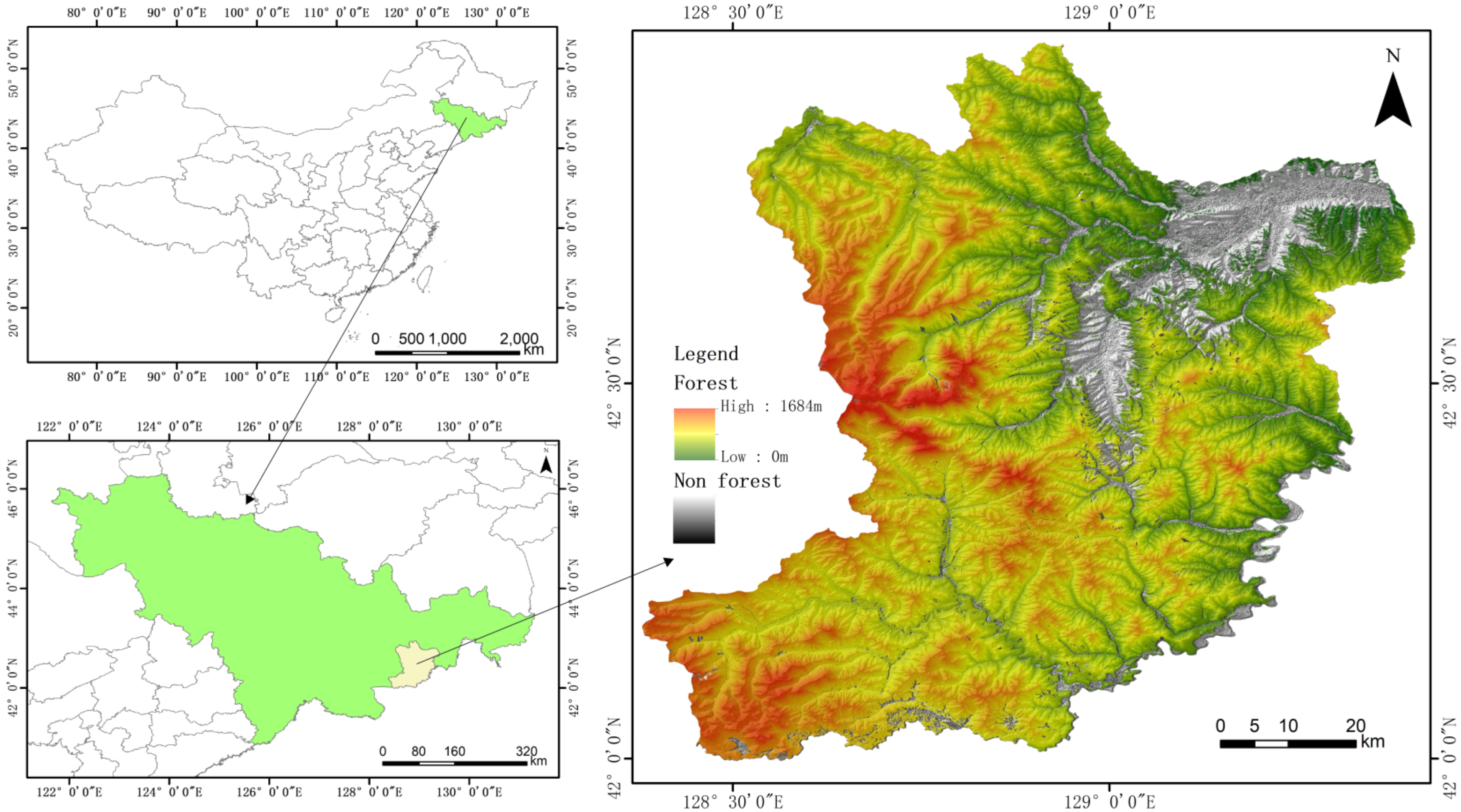
Figure 1. The study area. The forest area is overlaid with Shuttle Radar Topography Mission elevation data.
Forests 14 00107 g001
Figure 2. Flow diagram of tree species classification. The content bordered by a short dotted line represents the dominant tree species to be classified, and the content in the long dotted line box is several machine learning methods for comparison.
Forests 14 00107 g002
Figure 3. MCD43A4 images of the base date (May 19) and two predicted dates (May 28 and October 19).
Forests 14 00107 g003
Figure 4. Forest inventory data of the study area in 2016.
Forests 14 00107 g004
Figure 5. Distribution of sampling point data used in this study.
Forests 14 00107 g005
Figure 6. Real Landsat images on the base date and predicted dates.
Forests 14 00107 g006
Figure 7. RGB composition of the fusion results. The first and second rows are the MCD43A4, Landsat 8 OLI imagery, and the fused images of the three different methods (STARFM, FSDAF, and STNLFFM) on May 28 and October 19, respectively.
Forests 14 00107 g007
Figure 8. Correlation between the red and near-infrared bands on May 28 and October 19. (a) Correlation coefficient of the red band on May 28. (b) Correlation coefficient of the NIR band on May 28. (c) Correlation coefficient of the red band on October 19. (d) Correlation coefficient of the NIR band on October 19.
Forests 14 00107 g008
Figure 9. Overall accuracy and kappa coefficient of Experiments 1 and 2. (a) Experiment 1 (spectral features only). (b) Experiment 2 (spectral plus topographic features).
Forests 14 00107 g009aForests 14 00107 g009b
Figure 10. Confusion matrix for various classification methods: (a) KNN; (b) RF; (c) ANN; (d) LightGBM; (e) ensemble.
Forests 14 00107 g010
Figure 11. Classification results of forest tree species in Helong City based on the ensemble classifier and the optimal feature combination.
Forests 14 00107 g011
Table 1. Detailed information on remote sensing data used in this study.
Landsat 8MODIS
Date (all in 2016) 05-19, 05-28, 10-1905-19, 05-28, 10-19
03-21, …,10-28
Wavelength (nm)Blue
Green
Red
NIR
SWIR-1
SWIR-2
450–515
525–600
630–680
845–885
1560–1660
2100–2300
459–479
545–565
620–672
841–890
1628–1652
2105–2155
Resolution 30 m500 m
Repeat cycle 16 daysdaily
Table 2. Number of sampling points for each tree species.
Tree SpeciesTraining SamplesValidation Samples
Oak89462236
Larch67281682
Korean pine2170543
Pinus sylvestris49441236
Birch3145786
Table 3. The feature combinations of seven scenarios.
ExperimentInput DataNumber of Feature Variables
1Single-temporal surface reflectance (28 groups)6
2Single-temporal surface reflectance, topographic features (28 groups)9
310 fused images in spring60
49 fused images in summer54
59 fused images in autumn54
6All fused images in the time series168
7All fused images in the time series, topographic features171
83 cloud-free Landsat images on May 19, May 28, and October 19 201618
93 seasonal composite images of spring, summer, and autumn 201618
109 seasonal composite images of spring, summer, and autumn 2015, 2016, and 201754
Table 4. Main parameter settings of the base classifiers.
Base ClassifierParameterValue
KNNN_neighbors
N_jobs
3
−1
RFN_estimators
criterion
Max_depth
Min_samples_split
Min_samples_leaf
Max_features
N_jobs
870
‘gini’
None
2
1
‘sqrt’
−1
ANNHidden layer sizes
Learning rate
(400, 200, 100, 50)
0.0005
LightGBMN_estimators
Learning_rate
Num_leaves
Max_depth
N_jobs
1527
0.098
19
−1
−1
Table 5. Comparison of original Landsat imagery on the base date and predicted date.
DateCorrelation Coefficient
BlueGreenRedNIRSWIR1SWIR2Average
28 May 20160.96890.98420.97170.97500.98620.97200.9763
19 October 20160.81230.91200.80510.87120.91210.82510.8563
Table 6. Quantitative evaluation of spatiotemporal fusion accuracy.
DateMethodMetrics
CCRMSESSIMSAMERGAS
28 May 2016FSDAF0.97300.01650.99010.79422.3177
STARFM0.97440.01580.99070.79152.2258
STNLFFM0.97460.01560.99040.79212.2794
19 October 2016FSDAF0.91530.02580.97660.83443.2679
STARFM0.91350.02600.97640.84273.2861
STNLFFM0.92260.02480.97810.83293.1740
Table 7. Classification accuracy of different classifiers.
ExperimentKappa CoefficientOverall Accuracy
KNNRFANNLight
GBM
EnsembleKNNRFANNLight
GBM
Ensemble
10.52270.55610.56950.52520.58110.64560.67320.67830.64930.6895
20.58090.62760.61170.62290.65290.68840.72540.70860.72070.7420
30.69500.71410.75280.73670.76500.77100.78770.81440.80350.8241
40.69650.68260.74550.71110.75650.77260.76550.80830.78530.8178
50.67360.68790.73400.70660.75040.75560.76900.79910.78180.8092
60.72020.73030.76390.76010.78210.78970.79980.82150.82080.8368
70.72620.73380.77200.76930.78970.79430.80250.82900.82760.8432
80.55090.59150.58900.61210.63230.67020.70160.69150.71460.7292
90.52390.55810.58390.57270.61800.64970.68030.68790.68810.7184
100.63370.63170.67510.67360.72170.72750.73310.75960.76060.7945
Table 8. Producer precision, user precision, and F-value (%) for each category for different methods in Experiment 7 (italics indicate the best result).
ClassAccuracyKNNRFANNLightGBMEnsemble
OakUA77.38575.93079.90880.90682.315
PA81.02186.67086.26386.35386.444
F-value79.16180.94582.96483.54184.329
LarchUA82.10481.59685.49883.33387.130
PA76.20776.88079.40580.24780.920
F-value79.04579.16882.33981.76183.910
Korean PineUA69.35183.93470.16179.00379.903
PA61.87651.09869.46160.08065.868
F-value65.40163.52469.80968.25472.210
Pinus sylvestrisUA79.59679.34886.08081.51181.521
PA82.49484.81883.34686.05788.846
F-value81.01981.99284.69183.72385.026
BirchUA85.43694.01689.93292.03491.460
PA89.02480.89489.56687.66989.973
F-value87.19386.96389.74989.79990.710
Table 9. Producer precision, user precision, and F-value (%) for each category for different methods in the other nine experiments (italics indicate the best result).
ClassAccuracyKNNRFANNLightGBMEnsemble
OakUA69.47969.53376.18272.06475.114
PA77.0383.5776.71381.65282.612
F-value72.99875.85476.36176.51978.651
LarchUA74.05975.17376.06875.19878.092
PA69.19371.23774.25173.3174.994
F-value71.53673.14575.09774.23676.494
Korean PineUA58.70374.72860.11368.34271.236
PA44.40835.33755.41341.16449.706
F-value50.24147.4857.22751.06258.237
Pinus sylvestrisUA74.77875.21275.96876.2377.876
PA74.24177.55179.8178.52481.245
F-value74.46376.27477.75977.32379.493
BirchUA76.91685.9981.76283.9685.898
PA77.17668.95680.38673.01278.842
F-value77.01876.45281.00278.03282.189
Table 10. Comparison of our proposed ensemble classifier with the deep forest algorithm.
MethodOverall
Accuracy
Kappa
Coefficient
Deep Forest0.82560.7662
Ensemble Classifier0.84230.7911
Disclaimer/Publisher’s Note: The statements, opinions and data contained in all publications are solely those of the individual author(s) and contributor(s) and not of MDPI and/or the editor(s). MDPI and/or the editor(s) disclaim responsibility for any injury to people or property resulting from any ideas, methods, instructions or products referred to in the content.