Article

Assessing Phenological Shifts of Deciduous Forests in Turkey under Climate Change: An Assessment for Fagus orientalis with Daily MODIS Data for 19 Years

1
Department of Climate and Marine Sciences, Eurasia Institute of Earth Sciences, Istanbul Technical University, Maslak, Istanbul 34469, Turkey
2
Department of Geomatics Engineering, Faculty of Civil Engineering, Istanbul Technical University, Maslak, Istanbul 34469, Turkey
3
Department of Geography, Faculty of Letters, Istanbul University, Istanbul 34459, Turkey
*
Authors to whom correspondence should be addressed.
Forests 2023, 14(2), 413; https://doi.org/10.3390/f14020413
Submission received: 30 December 2022 / Revised: 5 February 2023 / Accepted: 10 February 2023 / Published: 17 February 2023
(This article belongs to the Special Issue Mapping Forest Vegetation via Remote Sensing Tools)

Abstract

:
Understanding how natural ecosystems are and will be responding to climate change is one of the primary goals of ecological research. Plant phenology is accepted as one of the most sensitive bioindicators of climate change due to its strong interactions with climate dynamics, and a vast number of studies from all around the world present evidence considering phenological shifts as a response to climatic changes. Land surface phenology (LSP) is also a valuable tool in the absence of observational phenology data for monitoring the aforementioned shift responses. Our aim was to investigate the phenological shifts of Fagus orientalis forests in Turkey by means of daily MODIS surface reflectance data (MOD09GA) for the period between 2002 and 2020. The normalized difference vegetation index (NDVI) was calculated for the entire Turkey extent. This extent was then masked for F. orientalis. These “Fagus pixels” were then filtered by a minimum of 80% spatial and an annual 20% temporal coverage. A combination of two methods was applied to the time series for smoothing and reconstruction and the start of season (SOS), end of season, and length of season parameters were extracted. Trends in these parameters over the 19-year period were analyzed. The results were in concert with the commonly reported earlier SOS pattern, by a Sen’s slope of −0.8 days year−1. Lastly, the relationships between SOS and mean, maximum and minimum temperature, growing degree days (GDD), and chilling hours (CH) were investigated. Results showed that the most significant correlations were found between the mean SOS trend and accumulated CH and accumulated GDD with a base temperature of 2 °C, both for the February–March interval. The immediate need for a phenological observation network in Turkey and its region is discussed.

1. Introduction

Phenology is the study of the seasonal timing of recurring life cycle events (i.e., “phenophases” [1] such as flowering or leaf unfolding) of plants and animals alike, and the drivers behind this timing and how these phenophases affect each other for the same species or between different species [2,3]. The rise of phenology as an integral part of global change research starts with this very quest. Quoting from Sparks and Carey [4], “In order to predict future responses of species to a changed climate we need first to discover how plants have responded to climate in the past.”
Plant phenology interacts both one sided and reciprocally with many biotic and abiotic factors such as climate [5,6,7]. It is a thoroughly studied fact that plant phenology is strongly under the effect of climate variables [8,9,10,11,12] and it is also able to affect climate dynamics through surface energy budget (e.g., surface roughness, albedo, etc.) and many other biophysical fluxes such as carbon sequestration and hydrological cycle (e.g., [13,14,15,16,17,18,19,20,21,22]). Consequently, phenology is defined as one of the most sensitive and easily observable bioindicators of climate change impacts in the literature (e.g., [23,24,25,26,27,28]) and unarguably has an important place in global environmental change research [29,30,31,32,33,34,35].
Traditionally, plant phenology data are obtained through field-based observations of individual plants [36,37], either by experts and/or volunteers of phenological networks [33]. However, to assess climate change impacts on the biosphere, as also noted by Parmesan and Yohe [5], analyses of global/regional response patterns are more important than individual-level responses because climate change itself is a global phenomenon. In order to comprehend the critical interplays between ecosystems and atmosphere, data from regional to global domains and at times from inaccessible areas are needed [38,39,40]. This exigence is far beyond the limits of field observations.
The advent of satellite remote sensing (SRS) gave an indisputable boost to ecological research [41,42,43,44], especially to phenology studies, to the point of the adoption of a neologism, “land surface phenology (LSP)” [45,46,47,48], which distinguishes the phenologies derived from SRS measurements from traditionally observed plant phenology. SRS provides datasets which have continuous near-global spatial coverage, high spatial resolution, and high imaging frequency options, and by repeated imaging of the same region, over long time periods, trend analysis through long time intervals is enabled by space-borne sensors [41,49,50,51,52,53]. Moreover, for locations where no observational data are present to track phenological responses (e.g., Turkey), LSP provides the much-needed estimations to fill the gaps in regional and global evaluations.
Phenological shifts (in LSP terminology; changes in the dates of the start and the end of seasons (SOS and EOS, respectively)) are one of the most commonly and globally reported responses to climate change [23,54]. The majority of these reports show that there is a spring advancement pattern ([40]; e.g., from Europe [55,56,57,58], from the U.S.A. [59], from North America [60], from Canada [61], from China [62], for the Northern Hemisphere [63], and from Korea [64], which commonly results in a longer growing season. Estimates of LSP studies also contribute to this deduction [65] in varying scales (e.g., [66,67,68,69,70].
The length of the growing season (LOS; the period between SOS and EOS) determines the timing and duration of carbon uptake for deciduous forests [15,71]. Although in the climate change mitigation context a prolongation in growing season length seems advantageous for carbon sequestration [16,71,72,73], SOS advancement may also have negative impacts, e.g., “false springs”, and plant growth in its vulnerable stages may be damaged by frosts [73,74,75], which poses an even greater threat to frost-sensitive species [76].
Deciduous broadleaf forests (DBFs) are frequently the focus of LSP research [77] as they present a clear and observable year-around phenological cycle [78] and the lifespan of trees enables consistent long-term analyses. Studies focused on deciduous forest cover vary scope-wise from data or method validation/comparison to investigating drivers behind phenological shifts (e.g., [79,80,81,82,83].
Turkey is located between 36°–42° N latitudes, in the easternmost Mediterranean Basin. Three intersecting phytogeographical regions [84,85,86], three seas bounding on three sides, diverse topography, and orographic positioning influences [87], which lead to varying climate attributes from Mediterranean to continental [88] as well as microclimatic effects, edaphic variability, and glacial refuges, result in a spectacular habitat, gene, and species diversity [89,90,91]. Turkey hosts around 10,000 vascular plant species with a high endemism ratio of 31–33% [84,92,93]. However, the Mediterranean Basin is identified as one of the most vulnerable locations to climate change by IPCC [94] and projections revealed that Turkey is expected to experience a temperature increase and alterations in precipitation [95,96,97]. Accurate management and conservation plans are a must and this goal requires a deeper understanding of if and how the natural ecosystems are, and will be, responding to climate change.
Despite the immediate climate threat and vulnerability of natural ecosystems, LSP studies in Turkey are almost exclusively limited to plants of agricultural and/or economic value, i.e., vegetation under human intervention. Turkey can be found as “a part of the study area” in European, Asian, or Northern Hemisphere LSP studies conducted with coarse–medium spatial resolution composite datasets (e.g., [98,99,100]). However, we could not find any previous study explicitly analyzing the long-term trends of phenological parameters and shifts of Turkey’s natural forest covers, with a clear phenological parameter extraction and sub-pixel information at species level.
To address the gap in the literature of phenological monitoring of natural vegetation covers in Turkey and contribute to what is known about deciduous forest phenology under climate change, we investigated if and how Fagus orientalis forests in Turkey have responded to climatic changes during the past 19 years (2002–2020) by assessing the trend of SOS, which was extracted from daily normalized difference vegetation index (NDVI) time series. With the interest of minimizing the mixed pixel effect, by means of a forest management map, pure stands of F. orientalis were filtered. We estimated multi-annual mean SOS, as well as EOS and LOS to present a better view of the seasonal patterns and investigated the effect of altitude and latitude on these phenological parameters, thus characterizing F. orientalis phenology in Turkey. We assessed the correlation between the annual mean SOS of all pixels and temperature-derived variables (growing degree days, chill hours, and mean, minimum, and maximum temperatures) to see if and how F. orientalis responded to significant changes in these variables over the study period. This study is the first LSP shift estimation for such a long time period and for such broad-scale deciduous forest covers in Turkey (all pure F. orientalis stand pixels in Turkey, after spatial and temporal coverage filtering), conducted by using daily MODIS data, except for our preliminary presentation in the earlier stages of this study [101]. Our results will contribute greatly to the regional and global LSP and forest phenology literature as well as provide a methodological baseline and a comparison yardstick for future LSP research on deciduous forest covers in Turkey and its region.

2. Materials and Methods

Google Earth Engine (GEE, [102]) was used to obtain surface reflectance and climate datasets for preprocessing surface reflectance data and for index calculations. The forest management map of Turkey was prepared as polygon masks in the QGIS environment. All other processes including extent masking for Fagus orientalis, time series smoothing and reconstruction, statistical analyses, and visualizations were conducted in the R environment (R version 3.2.0, R studio version 1.2.1335, [103]). All study steps including data acquisition and storage were conducted with a personal desktop PC running Windows 10. A work flow chart of the study is given in Figure 1.

2.1. Surface Reflectance Data Acquisition, Pre-Processing, and Index Calculations

2.1.1. Normalized Difference Vegetation Index—NDVI

Phenological research is mostly concentrated on plants “as their fixed location facilitates repeated observation” [61] which also applies to LSP research. Thus, vegetation indices (VIs) are frequently utilized in LSP studies [78,82,104]. As the recent review of Caparros-Santiago et al. [105] also presented, the most preferred vegetation index is the NDVI [106,107] in LSP studies. NDVI can be utilized as a proxy for climate change response of the the vegetation and greenness due to its strong connection with red reflectance and thus with fractional green biomass, evapotranspiration, NPP, LAI, unstressed vegetation conductance, fPAR, and canopy CO2 and H2O exchange activity [104,108,109,110,111]. NDVI is calculated as the difference between the red and near-infrared (NIR) bands normalized by their sum:
NDVI = (NIR − RED)/(NIR + RED)

2.1.2. Surface Reflectance Data, Preprocessing, and NDVI Calculation

MODIS products are one of the top preferred products in LSP research [105]. For the vast majority of LSP studies, MODIS composite index products for NDVI are utilized. Maximum value composite or MVC [112] is a method adopted for index products of MODIS to reduce the noise caused by cloud contamination, atmospheric variability of aerosols and dust, viewing angles, snow/ice, etc. [113,114]. However, there are concerns regarding composited products about their sensitivity to catch important phenological transition dates within the composited periods [81,115,116] while still having noise even after the MVC process 113. Considering these concerns, to calculate NDVI time series, the “MODIS/Terra Surface Reflectance Daily L2G Global 1 km and 500 m SIN Grid v006” (MOD09GA) [117] product at 500 m spatial resolution was chosen as the main dataset of this study.
Quality assessment (QA) layer information flags were used to exclude problematic pixels. We only included pixels, of which the QA flags are cloud state (clear), cloud shadow (no), MOD 35 Snow/Ice (no), aerosol quality (low, average, climatology), cirrus detected (no), and data quality (per band—highest). For all remaining pixels within the extent of Turkey, NDVI values were calculated according to Equation (1) and the daily NDVI time series were produced. At this step, a total of 13,870 images were processed.

2.2. Climate Data

To calculate accumulated GDDs (AGDD) and CHs, two data sets were downloaded via GEE: ERA5-Land Hourly—ECMWF Climate Reanalysis [118] and ERA5 Daily Aggregates—Latest Climate Reanalysis Produced by ECMWF [119]. Both datasets have a resolution of 0.25°. For the CH calculations the hourly dataset was utilized. For the GDD, the daily mean temperature was calculated by using the daily minimum and maximum temperature dataset. To extract the climate data for our study area, i.e., each study pixel, firstly, we determined the coordinates of the center of each pixel. Then, the corresponding pixels to these center coordinates in the climate data were extracted.

2.3. Forest Management Map and Fagus orientalis Masking

To filter pure stands of F. orientalis, we used a forest management map of Turkey.
Because all elements in a pixel are represented in one integrated sensor measurement/index value, one of the major limitations of LSP estimations is their dependency on sub-pixel information for a reliable interpretation. Especially utilizing spatially coarse–medium resolution data without sub-pixel information leads to over- and underestimations of season parameters as well as erroneous evaluations of the drivers behind the variability in estimations [120,121]. Thus, to avoid the effect of pixel heterogeneity to a degree, the selection of pure stands is important [122].
Due to its climatic sensitivity, beech is a frequently used species in phenological studies [123]. In Turkey, F. orientalis is found especially on the north-facing slopes of the mountain ranges in the Black Sea and Marmara regions, northern parts of Central Anatolia and Aegean regions, and Amanos mountains in the Mediterranean region as a relict species [124,125], and is a main component of North Anatolian mixed deciduous forests.
The determinant of our study area extent was the stand type masking (Figure 2) and the masked areas were presumptively expected to be, so to speak, “scattered all around Turkey” regarding the distribution of F. orientalis. Thus, we defined our initial study area as the entirety of Turkey and the actual study area, i.e., all pixels after the stand type, temporal and spatial masking, as “ExtentFagus” or study pixels.
Calculated NDVI raster for the entire extent of Turkey was masked with forest management plans which was filtered for pure stands of F. orientalis with highest canopy closedness (an option presented in the forest management map). With this step, a total of 78,147 pixels were masked for Fagus (see Figure 2). Then, a pixel coverage threshold of 80% was determined for the selected species and any pixel with a forest coverage lower than 80% was excluded from the study area (7027 pixels). Any pixel in the NDVI time series with an annual temporal coverage lower than 20% was also excluded from further analysis. These masking processes are the determinant of the study area, ExtentFagus (i.e., study pixels), which contains 5437 pixels.

2.4. Noise Reduction, Time Series Reconstruction, and Extraction of Phenological Parameters

As a level 2 product, MOD09GA is atmospherically corrected [126]; however, as expected of a dataset with such a fine temporal resolution, significantly high noise still remains. To handle the high noise and to reconstruct the daily NDVI time series, a combination of two methods, the Best Index Slope Extraction (BISE, [127]) and the Savitzky–Golay (S–G, [128]) filter, were applied [116,129].
BISE was used as the first level to reduce the remaining noise. Starting from the first day of the time series, BISE searches for and accepts the next point with a higher value than the previous point. It accepts lower values if there is no point in a pre-defined time period (sliding period) with a value that is higher than the predefined “threshold” percentage of the difference between the first low value and the previous high value. Should there be such a higher value, BISE accepts the higher value and rejects the lower point. For this study, the sliding period was assigned as 30 days and the threshold was set to 10%.
As the second step, to reconstruct the time series, an S–G filter was applied. The S–G filter is a simplified least-squares-fit convolution that can be inferred as a weighted moving average filter with weighting given as a polynomial of a certain degree [113,130]. To implement the S–G filter to NDVI time series, two parameters, m—the half-width of the smoothing window and d—the degree of the smoothing polynomial should be assigned. For this study, m was set to 7 and d was set to 2. The BISE and S–G application processes were realized with a R package called “phenex” [131]. After the smoothing and reconstruction, the main time series, which was used in the parameter extraction process, was produced.
To extract the phenological parameter of SOS per pixel, a piecewise logistic function fitting approach was applied to the time series [132]. The function fitting process was conducted with the “phenofit” R package [133]. Mean SOS dates of individual years and fitted curves marked on interannual mean raw time series are shown in Figure 3. For the purpose of presenting and interpreting the changes in growing season dynamics in a more understandable fashion, EOS values were also extracted for these 547 significant SOS pixels and LOS was calculated as the difference between EOS and SOS. As aforementioned, EOS and LOS parameters were not initially of interest in this paper, meaning that their interactions with temperature-derived variables were not assessed.

2.5. Trend Analysis of SOS

Because there is usually high positive autocorrelation between consecutive observations in NDVI time series, they often violate the assumption that “all ordinate values (y axis) should be mutually independent” of regression analysis which is frequently used for trend analysis in LSP studies [1,134]. Thus, trend analysis of SOS was conducted with a non-parametric Mann–Kendall (MK) test for each pixel. To calculate the slopes of the SOS, LOS, EOS, and temperature-derived variable trends, Sen’s Slope estimator was used. A negative Sen’s slope estimation indicates a decreasing trend while a positive estimation means an increasing one. Lastly, MK Tau presents a measure of strength. The closer Tau gets to +1, a stronger and increasing relationship is implied, while the closer it gets to −1, a stronger decreasing relationship is implied. Both the Mann–Kendall test and Sen’s Slope estimations were realized with a R package named “EnvStats” [135].
SOS trend directions of individual pixels and a breakdown of their significance levels (p < 0.05 and p ≥ 0.05) are shown in Figure 4. A total of 80.45% of the total pixels (4374 pixels) showed a negative trend with no significance while 10.01% (544 pixels) showed a significant negative trend (p < 0.05). A total of 9.49% of the pixels (516 pixels) showed a positive trend with no significance whereas 0.06% of the pixels (3 pixels) showed a significant positive trend. At this step, pixels which were not statistically significant (p ≥ 0.05) were excluded from the further analysis. With this exclusion, a total of 547 pixels were filtered for further analyses.

2.6. Analyzing Annual Mean SOS Correlation with Temperature-Derived Variables

We investigated the relationship between the trends of AGDD, CH, and mean, maximum, and minimum temperatures (Tmean, Tmax, and Tmin, respectively) and the trend of the mean SOS dates of 19 years to see (i) if any of these variables have a significant linear relationship with the mean SOS trend and (ii) linear relations between the mean SOS trend and variable/s and related interval/s with the highest significance. GDD was calculated as:
GDD = Tmax − Tmin/2 − Tbase
where Tmin and Tmax are minimum and maximum temperatures, respectively, and Tbase is the base threshold temperature for growth below which the investigated process does not occur [136]. CHs were calculated as the accumulated count of hours under the base temperature of 7.2 °C (approximately 45 °F [137,138,139]) within a given time interval.
Base temperature (Tbase) values ranging from 0 °C to 8 °C for AGDD calculations were examined for different time intervals. As D, J, F, M, and A stand for the months of December, January, February, March, and April, respectively, the AGDD intervals were day of year = DOY1 (as 1 January) − DOYSOS, JFMA, JFM, FMA, JF, FM, MA, J, F, M, and A. Intervals for CH were DJFM (December of the previous year), DJF, JFM, DJ, JF, FM, D, J, F, and M. The values of GDD Tbase were initially chosen based on their appearance frequency in the literature review, and then the list of values to examine was expanded for exploratory purposes.
A total of 139 combinations for Tmax, Tmin, Tmean, AGDD, and CH with different time intervals and different Tbase values for GDD were examined. Cases where (i) the variable has no significant correlation with the SOS trend and (ii) the variable has a significant correlation with the SOS trend but the variable itself does not have a significant trend over the study period were not presented in this paper; however, a table of all combinations and correlations, as well as which of the above-mentioned criterion the correlation was in, is provided in the Supplementary Materials. The latter criterion is crucial for our study because in temperate zones plant phenology is already considered to be driven primarily by temperature [140,141,142]. However, our focus was not on this relationship and instead aimed to assess if and how the “changes” in temperature-derived variables affect the shifts in the spring phenology of F. orientalis. Thus, a variable with no significant trend over the study period, although having a significant relationship with SOS, could not serve this aim.

3. Results and Discussion

Before discussing the findings, there are a few key points to be mentioned. We accept that results obtained from LSP studies, especially in the absence of observational phenology records to compare, should be taken as estimations and not as definitive results. With that being said, our aim was to estimate the shift between the interannual SOS dates by following LSP methodologies to interpret the estimations according to LSP terminology, to assess its interactions with temperature-derived variables, and to characterize Fagus phenology with multi-annual mean parameters in the absence of observational data. Thus, it is safe to say that this study stands as another good example of the utility of SRS data, albeit as a proxy, to monitor phenological parameters in domains where phenology observations for natural ecosystems are not available [143]. Without the advantages SRS brought into phenological research, phenological data from many countries, regions, etc., which does not have observational records, yet hold important and complementary clues for both ecological and climate change research, would be lacking in the global literature.
Long-term and continuous monitoring and assessments are of high importance in phenology as phenological shifts are not fixed processes; they do not only advance or delay but can also be observed to halt or reverse, slow down, or accelerate depending on the chosen time period [144,145,146]. Although 19 years can hardly be defined as “long term” in both statistical and natural processes contexts, to be able to work with daily data we chose the MOD09GA collection and to investigate the longest continuous period possible, we included the entire temporal coverage of the collection except for the aforementioned 2 years which were excluded.

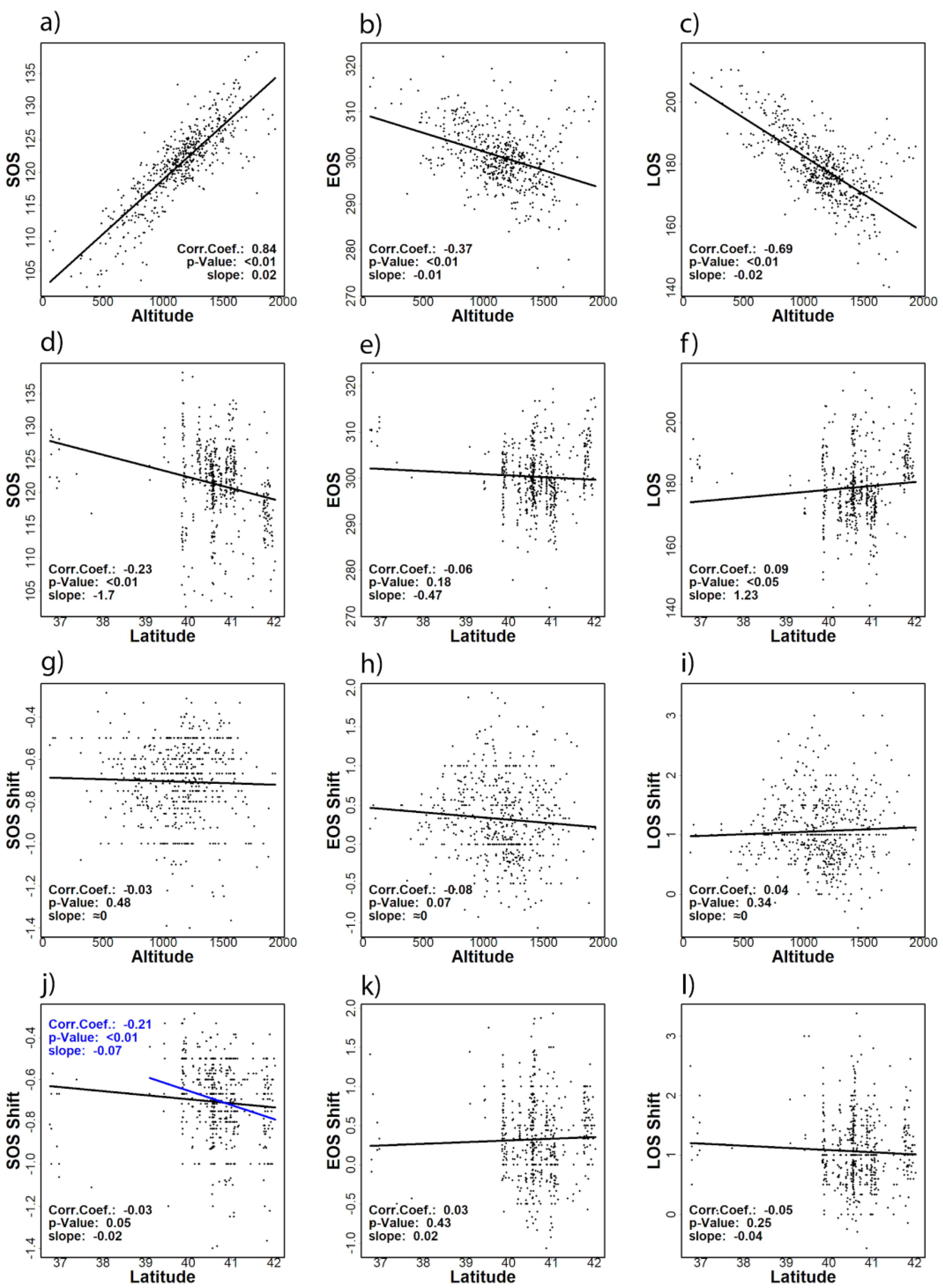
3.1. General Patterns of SOS, EOS Dates, and LOS

The distribution of mean SOS and EOS dates and LOS of individual pixels over the study period are shown in Figure 5. The multi-annual (2002–2020) mean SOS and EOS dates were DOY 121.21 and DOY 300.30, respectively, while the mean LOS was found to be 179.09 days. The earliest mean SOS was DOY 102.47 and the latest SOS was DOY 138.26, while the earliest and latest mean EOSs were DOY 271.89 and 322.94, respectively. The maximum LOS was 216 days and the minimum LOS was found to be 140.26 days.
We also investigated the possible distribution differences in phenological parameters and shifts, sourcing from latitudinal and altitudinal diversity (Figure 6). The latitudinal distribution of the SOS dates showed earlier SOS dates in the north and relatively later SOS dates in the south, represented as 1.7 days earlier per 1° (Figure 6d). The LOS was also found to be longer northwardly, represented as 1.23 days longer per 1° (Figure 6e), while for EOS no significant correlation was found.
Our investigation on the relationship of respective altitudes of the study pixels and the latitude showed that this pattern is due to the study pixels being distributed over relatively higher altitudes southwardly and lower altitudes in the north (Figure 7a,b). As shown in Figure 6a, SOS dates of study pixels and altitude have a strong positive relationship, i.e., at higher altitudes later SOS dates are seen while at lower altitudes SOS dates are earlier, as 2 days later per 100 m. upward. EOS was also found to have a significantly negative correlation with altitude, represented as 1 day earlier per 100 m. Similarly, LOS was found to have a significant negative correlation with altitude, represented as 2 days shorter per 100 m.

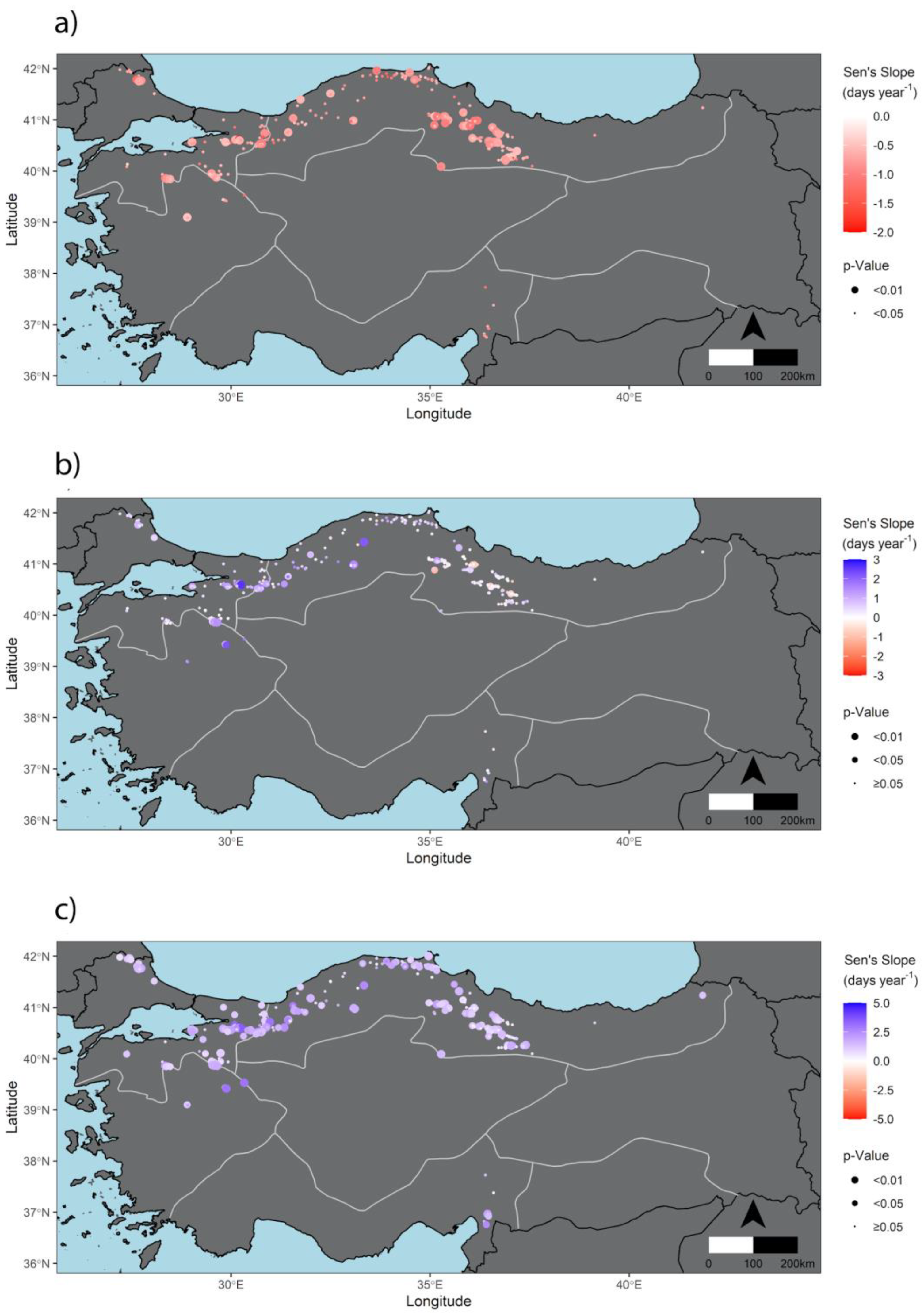
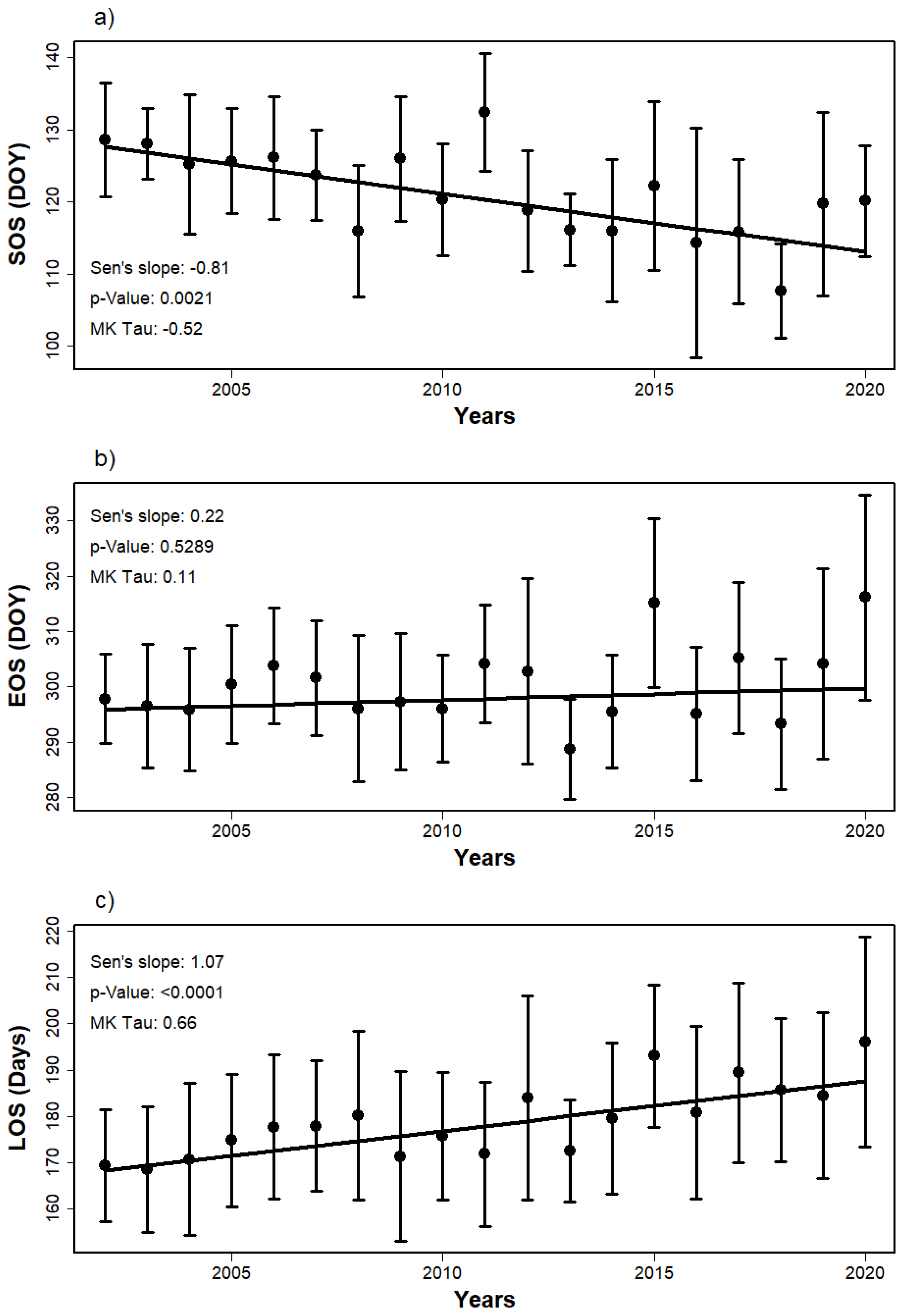
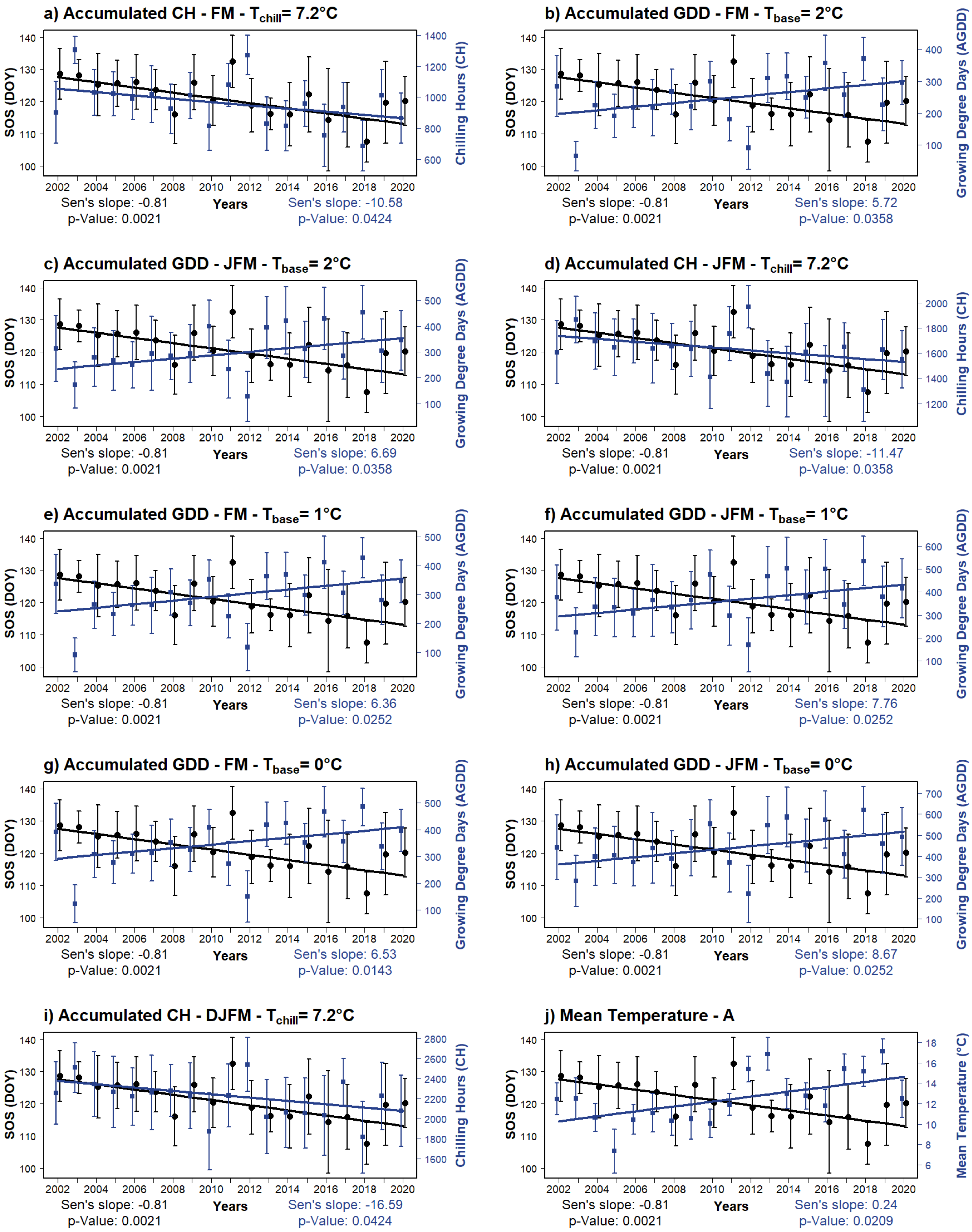
3.2. Trends of SOS, EOS, and LOS

Figure 8a shows the significant SOS trend and EOS (Figure 8b) and LOS (Figure 8c) trends of the same pixels over the study period. Unlike the mean SOS dates and mean LOS, no significant relationship between the SOS and LOS shifts and altitude was found (Figure 6g,i) as well as EOS (Figure 6h). For latitude on the other hand, a weak negative correlation was found which was apparent after latitude 39° N (Figure 6j), albeit not for all pixels, meaning that the shift increases northwardly, represented as −0.07 days per year−1. For the EOS and LOS shifts, no significant correlation with latitude was found (Figure 6k,l).
Trend analysis of mean SOS dates presented a Sen’s slope of −0.8 days per year−1 over the 19-year period, indicating an advancement of SOS, i.e., an earlier spring (Figure 9a). Mean EOS shift for the same pixels did not show a significant trend although a slightly increasing slope can be observed (Figure 9b). For LOS, a significant positive trend was found, implying a longer season by an average of 1.07 days per year−1 (Figure 9c) with an advancing SOS pattern.
The EOS is a more elusive parameter to catch in LSP studies than SOS, arguably this is so even for traditional phenology observations [74]. The reason is, unlike vernal measurements, many different factors may affect the band measurements for autumnal changes, e.g., autumnal litter, effect of soil wetness on the background, etc., [147] and unlike budburst it is a slow, continuous body of events [148] which makes it hard to detect even with traditional observations. Additionally, for deciduous trees, environmental factors which drive autumn phenological events, e.g., leaf fall, are less understood compared with vernal phenology [142]. Thus, a cautious approach is needed when interpreting EOS estimations [81], especially when there is no observational data to provide grounding.
The advancing spring pattern our estimates showed is in agreement with the majority of both traditional and land surface phenology studies conducted for Europe, Asia (two continents where Turkey resides in both), and the Northern Hemisphere ([55,56,57,58] and [62,63,64,134]). For example, in their study over western central Europe, utilizing both in situ and NDVI time series, Fu et al. ([144], Figure 3, 2000–2011 period) reported a leaf unfolding date advancement for Fagus sylvatica, with a trend between −0.5 and −1, over the period of 2000–2011. Stöckli and Vidale [10] found an earlier (−0.54 days per year−1) and longer (by 0.96 days per year−1) growing seasons for Europe, especially central Europe for the period of 1982–2000. For the Northern Hemisphere, Jeong et al. [145] found an advancing SOS by −5.2 days per year−1 for the period 1982–1999, albeit this advancement was found to be slowed down for the 2000–2008 period (advancement by −0.2 days per year−1).
According to the satellite-derived (AVHHR-NDVI) budburst timing evaluation in [79] made for beech and oak, the SOS dates our estimations produced (Figure 3) which are about late April–early May are realistic. Our SOS date estimates for the years 2015 (DOY 122) and 2016 (DOY 114) also show high accordance with the ground-based sensor-obtained green-up date intervals for beech (2015; DOY 115–129 and 2016; DOY 114–129) in [149] where they validated different satellite phenology products (MODIS Terra/Aqua and Sentinel 2A) by multi-sensor ground measurements. It is worth noting that, despite the fact that phenological parameters extracted from satellite data (e.g., SOS) are commonly found either earlier or later than the ground-observation-based (sensors or traditional) bud-burst/green-up dates by varying time scales from days to weeks, our results are in concert with the dates in the reviewed literature. However, due to the fact that geography plays a crucial role in phenology, even for the same species, different SOS dates are observed for different locations, which should also be noted.

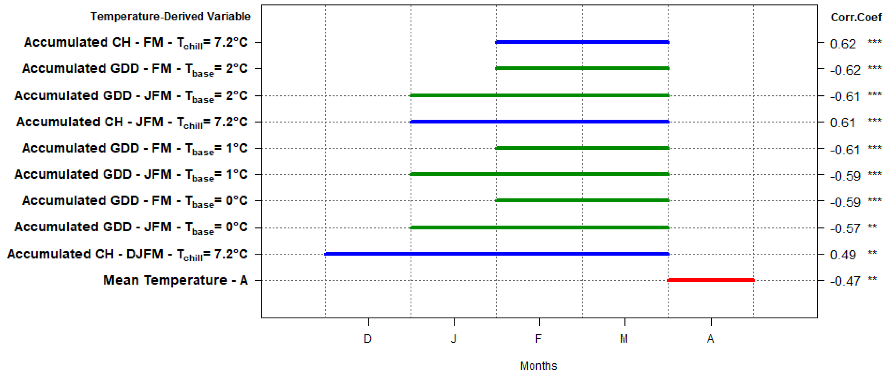
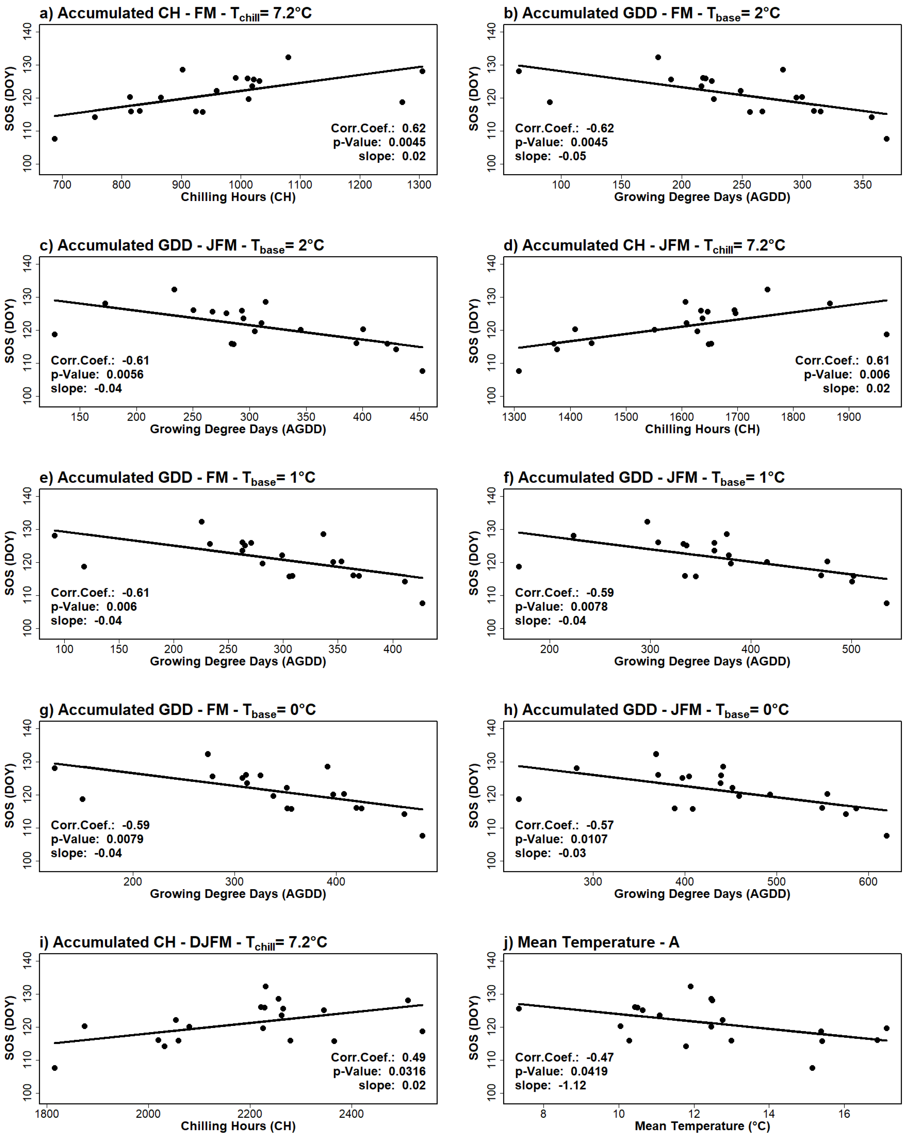
3.3. Correlations with Temperature-Derived Variables

All statistically significant correlations between the mean SOS trend and temperature-derived variable/interval combinations, ranked by correlation coefficients (from top to bottom; the highest to the lowest), are shown in Figure 10 and plots of the correlations with the mean SOS trend are given in Figure 11.
As seen in Figure 10, the accumulated CHs for February–March and AGDD for the FM interval with a Tbase value of 2 °C have the most significant relationships with SOS (2 days later per 100 CH and 5 days earlier per 100 AGDD, respectively). Results given in the figure suggest a strong FM dominance over the rest of the time intervals for both GDD and CH. Individually, however, neither February nor March presented a significant relationship with SOS for Tmean, Tmax, and Tmin, and CH or GDD with any Tbase values examined.
In their observational-records-based study on four deciduous species across Europe, Chmielewski and Rötzer [55] also found that the beginning of the season is significantly influenced by February, March, and April temperatures, and according to their results, February to March temperatures are decisive for the annual start of spring in Europe. The authors of [150] conducted a similar study that also integrated sensor data and studied four common tree species across Europe. They found that the SOS date for beech (Fagus sylvatica) was significantly influenced by the mean temperature of the month in which SOS occurred and the preceding month, as well as the mean temperature of the month in which SOS occurred together with the two preceding months. Although we did not find a significant relationship between the mean SOS trend and the FMA or February intervals, our results also indicate a strong February–March dominance over the rest of the time intervals for both CH and GDD. Moreover, in concert with their findings, the mean temperature in April was the only individual-month interval as well as the only mean temperature variable which showed a significant correlation with the mean SOS trend, as the SOS occurs 1.12 days earlier per 1 °C (Figure 11j). This is important because according to our estimations, as shown in Figure 3, for F. orientalis, the mean SOS occurred around late April–early May over the study period.
Chilling requirements of a species is one of the factors that affect the response to temperature changes, together with temperature forcing and photoperiod [151]. To break dormancy, a period of exposure to cold temperatures, i.e., fulfilling the chilling requirements is needed for plants [137,152]. Many studies reported that unmet chilling requirements may lead to delaying of budburst and leaf out dates and to a shorter growing season [152,153,154]. Thus, although the majority of LSP and observational phenology studies focus on the increasing temperature, finding a high correlation between the decreasing CHs (see Figure 10), especially for CHs in winter months, and the mean SOS trend was not unexpected. However, the nature of the correlation, i.e., an advancing spring start while CH decreases, is interesting (Figure 12a,d,i). A possible explanation for the commonly reported spring advancement despite the insufficient chilling due to the increasing temperatures, which is considered as a delaying factor for SOS, has been hypothesized as the impact of this delay being minor compared with vernal temperature advances [152,155].
The CH in preceding months has a higher correlation with SOS compared with longer intervals which are further than the SOS date (Figure 11a,d,i). This pattern is also similar for GDD and GDD correlation with SOS weakening as the TBase decreases from 2 °C to 0 °C (Figure 11b,c,e–h).

3.4. An Earlier Spring and Prolonging Season: What Do These Mean?

From an ecosystem services point of view, many studies conclude that a longer growing season has a high importance for ecosystem productivity and it contributes to achieve a stronger net primary productivity and carbon uptake in temperate and boreal forest ecosystems, although some contradicting results were also reported [17,21,134]. On the species level, however, there are some other points of concern. One of them is mismatches between species in the phenology context. Mismatches happen when the time of a species’ high demand for a resource does not match the time of that particular resource being abundant [156]. Not all species change their phenologies at the same time or the same rate, and some may not even change their phenology as a response to climate or other environmental changes at all.
In a narrower context, one of the main concerns about an advancing spring and earlier leaf unfolding of trees is the impacts of late spring frosts. Late spring frosts are defined to occur after the first leaf-out and are of crucial importance as trees are most vulnerable to frosts during the initial stages of leaf emergence after the dormancy period [74,157]. Although increasing temperatures may seem to decrease late spring frost events, an advanced leaf unfolding and the following short period of up to 2 weeks of low-frost resistance until leaf hardening will also take place earlier [74,158]. Late spring frosts may damage beech growth and in some cases may even cause a total loss of leaves.

3.5. Limitations of the Study

The most prominent limitation of this study, and in a sense why it was carried out to assess SRS as an alternative method to monitor phenology and phenological shifts, is the absence of observational data to validate and/or compare our results. Hence, we tried to focus more on the patterns rather than the numbers presented by our estimations.
By utilizing sensor data with such a fine temporal resolution considering the aforementioned concerns on the sensitivity of composite datasets to catch phenophases, we traded off a finer spatial resolution, which is a frequently mentioned trade-off for sensor data. The impact of the spatial resolution of the MOD09GA collection (500 m) manifests itself the most, probably in pixel heterogeneity, as each band measurement value of a pixel represents all of the elements that the pixel contains, such as soil and understory [37]. The understory elements, for example, are known to green-up generally earlier than the main tree species in the same pixel. Testa et al. [81] found that the understory in Fagus sylvatica stands reached its 90% level of leaf onset at the time F. sylvatica only reached its 10%. Especially with coarse/medium resolution data, such as MOD09GA, these elements may lead to erroneous estimations. Thus, to keep this effect to a minimum, we used forest management plans and masked our initial NDVI pixels for Fagus-pure stands and with the highest canopy closedness only. Then, we filtered these Fagus-only pixels by a minimum spatial coverage of 80% and any pixel with a Fagus coverage less than 80% was excluded. This filter limit can go up to 100% (e.g., see [122]) and there are also examples of studies where it was set as 60% (e.g., see [159]). To work with a reasonable count of pixels and to have pixels from as many different regions as possible while keeping pixel heterogeneity minimal, an optimal 80% was set as the minimum coverage limit. Moreover, although our aim was to investigate the possible phenological shift patterns for “deciduous forests”, we went beyond and worked at the species level, i.e., F. orientalis, to be confident, as much as possible, in the estimations made for the deciduous forest, and the unwanted effect of other elements was minimized.
The resolution difference between the sensor data (500 m) and the climate datasets (0.25°) must also be mentioned as it is inevitable to have potential discrepancies.
Latitudinal gradients are usually more prominent in larger scales, e.g., regional and continental scales, and Turkey has a relatively narrow latitudinal width and the distribution of pure F. orientalis stands is also a narrow range in the north. Although we also included a latitudinal analysis in our study, this would be the reason why an emphasized latitudinal gradient was not found. Due to the cloud cover, a characteristic of the regional climate which interrupts band measurements for a majority of days of the year, many Fagus pixels from the eastern Black Sea region were filtered by the QA layer and could not be used in the study.
Because temperature is considered to be the dominant driver of phenology for temperate-zone deciduous forests [142], we investigated the relationship between SOS shift and temperature-derived variables. There are many other factors not covered in this paper that can help explain our findings more in depth such as precipitation and photoperiod, which are also considered among the main drivers of plant phenology. However, for this paper we aimed for a synoptic view of the possible shift patterns and distributions of phenological parameters and to present a workflow to work with daily MOD09GA data, to constitute a baseline; some of the factors aforementioned will be included in the next steps of our study.

4. Conclusions

SRS provides ecologists with long-term and continuous datasets which are collected objectively from local to global scales. Narrowing down the ecology title to phenology and phenology monitoring, SRS stands as a powerful means for observing the large- to local-scale patterns alike, especially for regions or ecosystems where observational data are not available. By means of SRS data, we assessed the SOS shift of F. orientalis pixels over the period of 2002–2020, detected the significant trends and assessed their directions, distributions, and the resulting vernal shift pattern (advancing SOS), and investigated the relationship between the mean SOS shift and temperature-derived variables and also characterized the phenology of F. orientalis in Turkey. As Turkey does not have a phenological observation network for natural ecosystems, this study is another good example of the advantages SRS brings to phenological research.
With that being said, it must be emphasized that the results from the LSP studies, even for the same species and same location, may vary depending on many factors such as the preferred sensor’s specifications, temporal and spatial resolution of the sensor data, methods used for time series reconstruction/noise reduction and phenological parameter extraction, study period length (which is usually limited by the temporal coverage of the data), etc. Thus, for future LSP studies on deciduous forests in Turkey and the region, we recommend studies on varying sizes of study areas, focusing on both different mixtures of deciduous tree species and, if possible, single species as well, with different sensor data (data with different temporal and spatial resolution as well as different temporal coverage) and with higher resolution climate datasets to enrich the literature with comparable results.
Although our results were in accordance with the existing literature and this study itself is proof of the evident benefits of SRS for ecological research and phenology monitoring, estimations based on SRS are not a replacement for observational phenology data/records. To be able to go beyond the general patterns, in the current state of LSP research, these estimations need validation to an extent. Considering the spectacular biodiversity Turkey has, the climate projections aforementioned, and the shift pattern we presented in this study on this opportunity, we underline the need for a phenology network to be established in Turkey, either as a citizen-science-based, traditional observation network to track the phenologies of prioritized/key species or as a network of near-surface phenology instruments (e.g., phenocams) to monitor natural vegetation covers and to share the records as open-access data. A cooperative, regional network would also be a good option as it would facilitate joint research projects and better information and experience sharing for the scientists in the field. We strongly believe that it will greatly benefit ecological research, not only in Turkey but also in the region.

Supplementary Materials

The following supporting information can be downloaded at: https://www.mdpi.com/article/10.3390/f14020413/s1, Table S1: Assessed climate variables over the study period (2002–2020).

Author Contributions

Conceptualization, T.Ş. and H.N.D.; methodology, T.Ş., O.K. and F.B.B.; formal analysis, T.Ş. and O.K.; data curation, T.Ş. and O.K.; writing—original draft preparation, T.Ş.; writing—review and editing, T.Ş., F.B.B., M.A. and H.N.D.; visualization, T.Ş. and O.K. All authors have read and agreed to the published version of the manuscript.

Funding

This research received no external funding. This study is a part of the Ph.D. thesis of Ş.T. and was not funded as a project. However, during her studies, Ş.T. was awarded with the 100/2000 Doctorate Scholarship by the Turkish Council of Higher Education.

Data Availability Statement

All data used in this study are open access except for the forest management plans. The surface reflectance and the climate data sets can be downloaded via the links provided in the references.

Acknowledgments

We would like to thank Sedat Avcı for his intense support of this study.

Conflicts of Interest

The authors declare no conflict of interest.

References

  1. De Beurs, K.M.; Henebry, G.M. A land surface phenology assessment of the northern polar regions using MODIS reflectance time series. Can. J. Remote Sens. 2010, 36, S87–S110. [Google Scholar] [CrossRef]
  2. Lieth, H. (Ed.) Phenology and Seasonality Modeling; Springer: Berlin/Heidelberg, Germany, 1974; Volume 8. [Google Scholar]
  3. Rathcke, B.; Lacey, E.P. Phenological patterns of terrestrial plants. Annu. Rev. Ecol. Syst. 1985, 16, 179–214. [Google Scholar] [CrossRef]
  4. Sparks, T.H.; Carey, P.D. The Responses of Species to Climate Over Two Centuries: An Analysis of the Marsham Phenological Record, 1736–1947. J. Ecol. 1995, 83, 321–329. [Google Scholar] [CrossRef]
  5. Parmesan, C.; Yohe, G. A globally coherent fingerprint of climate change impacts across natural systems. Nature 2003, 421, 37–42. [Google Scholar] [CrossRef]
  6. Schwartz, M.D. Phenology and Springtime Surface-Layer Change. Mon. Weather Rev. 1992, 120, 2570–2578. [Google Scholar] [CrossRef]
  7. Zhang, X.; Tarpley, D.; Sullivan, J.T. Diverse responses of vegetation phenology to a warming climate. Geophys. Res. Lett. 2007, 34. [Google Scholar] [CrossRef]
  8. Diez, J.M.; Ibáñez, I.; Miller-Rushing, A.J.; Mazer, S.J.; Crimmins, T.M.; Crimmins, M.A.; Bertelsen, C.D.; Inouye, D.W. Forecasting phenology: From species variability to community patterns. Ecol. Lett. 2012, 15, 545–553. [Google Scholar] [CrossRef] [Green Version]
  9. Peñuelas, J.; Filella, I. Responses to a Warming World. Science 2001, 294, 793–795. [Google Scholar] [CrossRef]
  10. Stöckli, R.; Vidale, P.L. European plant phenology and climate as seen in a 20-year AVHRR land-surface parameter dataset. Int. J. Remote Sens. 2004, 25, 3303–3330. [Google Scholar] [CrossRef]
  11. Chidumayo, E.N. Climate and Phenology of Savanna Vegetation in Southern Africa. J. Veg. Sci. 2001, 12, 347–354. [Google Scholar] [CrossRef]
  12. Pau, S.; Wolkovich, E.M.; Cook, B.I.; Davies, T.J.; Kraft, N.J.B.; Bolmgren, K.; Betancourt, J.L.; Cleland, E.E. Predicting phenology by integrating ecology, evolution and climate science. Glob. Chang. Biol. 2011, 17, 3633–3643. [Google Scholar] [CrossRef]
  13. Wilson, K.B.; Baldocchi, D.D. Seasonal and interannual variability of energy fluxes over a broadleaved temperate deciduous forest in North America. Agric. For. Meteorol. 2000, 100, 1–18. [Google Scholar] [CrossRef]
  14. Fitzjarrald, D.R.; Acevedo, O.C.; Moore, K.E. Climatic Consequences of Leaf Presence in the Eastern United States. J. Clim. 2001, 14, 598–614. [Google Scholar] [CrossRef]
  15. Keeling, C.D.; Chin, J.F.S.; Whorf, T.P. Increased activity of northern vegetation inferred from atmospheric CO2 measurements. Nature 1996, 382, 146–149. [Google Scholar] [CrossRef]
  16. Churkina, G.; Schimel, D.; Braswell, B.H.; Xiao, X. Spatial analysis of growing season length control over net ecosystem exchange. Glob. Chang. Biol. 2005, 11, 1777–1787. [Google Scholar] [CrossRef]
  17. Gu, L.; Post, W.M.; Baldocchi, D.; Black, T.A.; Verma, S.B.; Vesala, T.; Wofsy, S.C. Phenology of vegetation photosynthesis. In Phenology: An Integrative Environmental Science; Springer: Dordrecht, The Netherlands, 2003; pp. 467–485. [Google Scholar]
  18. Bounoua, L.; DeFries, G.; Collatz, G.J.; Sellers, P.J.; Khan, H. Effects of land cover conversion on surface climate. Clim. Change 2002, 52, 29–64. [Google Scholar] [CrossRef]
  19. Peñuelas, J.; Rutishauser, T.; Filella, I. Phenology Feedbacks on Climate Change. Science 2009, 324, 887–888. [Google Scholar] [CrossRef] [Green Version]
  20. Pielke Sr, R.A. Influence of the spatial distribution of vegetation and soils on the prediction of cumulus convective rainfall. Rev. Geophys. 2001, 39, 151–177. [Google Scholar] [CrossRef] [Green Version]
  21. Richardson, A.D.; Black, T.A.; Ciais, P.; Delbart, N.; Friedl, M.A.; Gobron, N.; Hollinger, D.Y.; Kutsch, W.L.; Longdoz, B.; Luyssaert, S.; et al. Influence of spring and autumn phenological transitions on forest ecosystem productivity. Philos. Trans. R. Soc. B Biol. Sci. 2010, 365, 3227–3246. [Google Scholar] [CrossRef] [Green Version]
  22. Gonsamo, A.; Chen, J.M.; Wu, C.; Dragoni, D. Predicting deciduous forest carbon uptake phenology by upscaling FLUXNET measurements using remote sensing data. Agric. For. Meteorol. 2012, 165, 127–135. [Google Scholar] [CrossRef]
  23. Walther, G.-R.; Post, E.; Convey, P.; Menzel, A.; Parmesan, C.; Beebee, T.J.C.; Fromentin, J.-M.; Hoegh-Guldberg, O.; Bairlein, F. Ecological responses to recent climate change. Nature 2002, 416, 389–395. [Google Scholar] [CrossRef] [PubMed]
  24. Rosenzweig, C.; Casassa, G.; Karoly, D.J.; Imeson, A.; Liu, C.; Menzel, A.; Rawlins, S.; Root, T.L.; Seguin, B.; Tryjanowski, P. Assessment of Observed Changes and Responses in Natural and Managed Systems. In Contribution of Working Group II to the Fourth Assessment Report of the Intergovernmental Panel on Climate Change; Parry, M.L., Canziani, O.F., Palutikof, J.P., van der Linden, P.J., Hanson, C.E.., Eds.; Cambridge University Press: Cambridge, UK, 2007; pp. 79–131. [Google Scholar] [CrossRef]
  25. Menzel, A.; Sparks, T.H.; Estrella, N.; Koch, E.; Aasa, A.; Ahas, R.; Alm-Kübler, K.; Bissolli, P.; Braslavská, O.; Briede, A.; et al. European phenological response to climate change matches the warming pattern. Glob. Chang. Biol. 2006, 12, 1969–1976. [Google Scholar] [CrossRef]
  26. Schwartz, M.D.; Reed, B.C.; White, M.A. Assessing satellite-derived start-of-season measures in the conterminous USA. Int. J. Climatol. A J. R. Meteorol. Soc. 2002, 22, 1793–1805. [Google Scholar] [CrossRef]
  27. Badeck, F.-W.; Bondeau, A.; Böttcher, K.; Doktor, D.; Lucht, W.; Schaber, J.; Sitch, S. Responses of spring phenology to climate change. New Phytol. 2004, 162, 295–309. [Google Scholar] [CrossRef]
  28. Migliavacca, M.; Sonnentag, O.; Keenan, T.F.; Cescatti, A.; O’Keefe, J.; Richardson, A.D. On the uncertainty of phenological responses to climate change, and implications for a terrestrial biosphere model. Biogeosciences 2012, 9, 2063–2083. [Google Scholar] [CrossRef] [Green Version]
  29. White, M.A.; Brunsell, N.; Schwartz, M.D. Vegetation phenology in global change studies. In Phenology: An Integrative Environmental Science; Springer: Dordrecht, The Netherlands, 2003; pp. 453–466. [Google Scholar]
  30. Cleland, E.E.; Chuine, I.; Menzel, A.; Mooney, H.A.; Schwartz, M.D. Shifting plant phenology in response to global change. Trends Ecol. Evol. 2007, 22, 357–365. [Google Scholar] [CrossRef]
  31. Morellato, L.P.C.; Alberton, B.; Alvarado, S.T.; Borges, B.; Buisson, E.; Camargo, M.G.G.; Cancian, L.F.; Carstensen, D.W.; Escobar, D.F.; Leite, P.T.; et al. Linking plant phenology to conservation biology. Biol. Conserv. 2016, 195, 60–72. [Google Scholar] [CrossRef] [Green Version]
  32. Chuine, I.; Beaubien, E.G. Phenology is a major determinant of tree species range. Ecol. Lett. 2001, 4, 500–510. [Google Scholar] [CrossRef] [Green Version]
  33. Menzel, A. Phenology: Its Importance to the Global Change Community. Clim. Chang. 2002, 54, 379–385. [Google Scholar] [CrossRef]
  34. Wolfe, D.W.; Schwartz, M.D.; Lakso, A.N.; Otsuki, Y.; Pool, R.M.; Shaulis, N.J. Climate change and shifts in spring phenology of three horticultural woody perennials in northeastern USA. Int. J. Biometeorol. 2004, 49, 303–309. [Google Scholar] [CrossRef]
  35. Kariyeva, J.; Van Leeuwen, W.J.D. Environmental Drivers of NDVI-Based Vegetation Phenology in Central Asia. Remote Sens. 2011, 3, 203–246. [Google Scholar] [CrossRef] [Green Version]
  36. Brügger, R.; Dobbertin, M.; Kräuchi, N. Phenological variation of forest trees. In Phenology: An Integrative Environmental Science; Springer: Dordrecht, The Netherlands, 2003; pp. 255–267. [Google Scholar]
  37. Reed, B.C.; Brown, J.F.; Vanderzee, D.; Loveland, T.R.; Merchant, J.W.; Ohlen, D.O. Measuring phenological variability from satellite imagery. J. Veg. Sci. 1994, 5, 703–714. [Google Scholar] [CrossRef]
  38. Moulin, S.; Kergoat, L.; Viovy, N.; Dedieu, G. Global-Scale Assessment of Vegetation Phenology Using NOAA/AVHRR Satellite Measurements. J. Clim. 1997, 10, 1154–1170. [Google Scholar] [CrossRef]
  39. Nagai, S.; Nasahara, K.N.; Inoue, T.; Saitoh, T.M.; Suzuki, R. Review: Advances in in situ and satellite phenological observations in Japan. Int. J. Biometeorol. 2015, 60, 615–627. [Google Scholar] [CrossRef] [Green Version]
  40. Linderholm, H.W. Growing season changes in the last century. Agric. For. Meteorol. 2006, 137, 1–14. [Google Scholar] [CrossRef]
  41. Pettorelli, N.; Vik, J.O.; Mysterud, A.; Gaillard, J.-M.; Tucker, C.J.; Stenseth, N.C. Using the satellite-derived NDVI to assess ecological responses to environmental change. Trends Ecol. Evol. 2005, 20, 503–510. [Google Scholar] [CrossRef] [PubMed]
  42. Pettorelli, N.; Laurance, W.F.; O’Brien, T.G.; Wegmann, M.; Nagendra, H.; Turner, W. Satellite remote sensing for applied ecologists: Opportunities and challenges. J. Appl. Ecol. 2014, 51, 839–848. [Google Scholar] [CrossRef]
  43. Kerr, J.T.; Ostrovsky, M. From space to species: Ecological applications for remote sensing. Trends Ecol. Evol. 2003, 18, 299–305. [Google Scholar] [CrossRef]
  44. Piao, S.; Fang, J.; Zhou, L.; Ciais, P.; Zhu, B. Variations in satellite-derived phenology in China’ s temperate vegetation. Glob. Change Biol. 2006, 12, 672–685. [Google Scholar] [CrossRef]
  45. Henebry, G.M.; Su, H. Observing spatial structure in the Flint Hills using AVHRR maximum biweekly NDVI composites. In Proceedings of the 14th North American Prairie Conference, Manhattan, AR, USA, 12–16 July 1994; Kansas State University Press: Manhattan, KS, USA, 1995. Available online: http://images.library.wisc.edu/EcoNatRes/EFacs/NAPC/NAPC14/reference/econatres.napc14.ghenebry.pdf (accessed on 7 April 2020).
  46. Henebry, G.M.; de Beurs, K.M. Remote sensing of land surface phenology: A prospectus. In Phenology: An Integrative Environmental Science; Springer: Dordrecht, The Netherlands, 2013; pp. 385–411. [Google Scholar]
  47. Friedl, M.; Henebry, G.; Reed, B.; Huete, A.; White, M.; Morisette, J.; Nemani, R.; Zhang, X.; Myneni, R. Land Surface Phenology. A Community White Paper Requested by NASA; 10 April 2006. Available online: http://cce.nasa.gov/mtg2008_ab_presentations/Phenology_Friedl_whitepaper.pdf (accessed on 22 March 2022).
  48. White, M.A.; de Beurs, K.M.; Didan, K.; Inouye, D.W.; Richardson, A.D.; Jensen, O.P.; Lauenroth, W.K. Intercomparison, interpretation, and assessment of spring phenology in North America estimated from remote sensing for 1982–2006. Glob. Chang. Biol. 2009, 15, 2335–2359. [Google Scholar] [CrossRef]
  49. Shabanov, N.; Wang, Y.; Buermann, W.; Dong, J.; Hoffman, S.; Smith, G.; Tian, Y.; Knyazikhin, Y.; Myneni, R. Effect of foliage spatial heterogeneity in the MODIS LAI and FPAR algorithm over broadleaf forests. Remote Sens. Environ. 2003, 85, 410–423. [Google Scholar] [CrossRef] [Green Version]
  50. Roughgarden, J.; Running, S.W.; Matson, P.A. What Does Remote Sensing Do For Ecology? Ecology 1991, 72, 1918–1922. [Google Scholar] [CrossRef]
  51. Pettorelli, N.; Schulte Bühne, H.; Shapiro, A.C.; Glover-Kapfer, P. Satellite Remote Sensing for Conservation. WWF Conserv. Technol. Ser. 2018, 1, 124. [Google Scholar]
  52. Pettorelli, N.; Bühne, H.S.T.; Tulloch, A.; Dubois, G.; Macinnis-Ng, C.; Queirós, A.M.; Keith, D.A.; Wegmann, M.; Schrodt, F.; Stellmes, M.; et al. Satellite remote sensing of ecosystem functions: Opportunities, challenges and way forward. Remote Sens. Ecol. Conserv. 2017, 4, 71–93. [Google Scholar] [CrossRef]
  53. Ives, A.R.; Zhu, L.; Wang, F.; Zhu, J.; Morrow, C.J.; Radeloff, V.C. Statistical inference for trends in spatiotemporal data. Remote Sens. Environ. 2021, 266, 112678. [Google Scholar] [CrossRef]
  54. Parmesan, C.; Hanley, M.E. Plants and climate change: Complexities and surprises. Ann. Bot. 2015, 116, 849–864. [Google Scholar] [CrossRef] [PubMed]
  55. Chmielewski, F.-M.; Rötzer, T. Response of tree phenology to climate change across Europe. Agric. For. Meteorol. 2001, 108, 101–112. [Google Scholar] [CrossRef]
  56. Menzel, A.; Fabian, P. Growing season extended in Europe. Nature 1999, 397, 659. [Google Scholar] [CrossRef]
  57. Ahas, R.; Aasa, A.; Menzel, A.; Fedotova, V.G.; Scheifinger, H. Changes in European spring phenology. Int. J. Climatol. A J. R. Meteorol. Soc. 2002, 22, 1727–1738. [Google Scholar] [CrossRef]
  58. Gordo, O.; Sanz, J.J. Long-term temporal changes of plant phenology in the Western Mediterranean. Glob. Chang. Biol. 2009, 15, 1930–1948. [Google Scholar] [CrossRef]
  59. Cayan, D.R.; Dettinger, M.D.; Kammerdiener, S.A.; Caprio, J.M.; Peterson, D.H. Changes in the Onset of Spring in the Western United States. Bull. Am. Meteorol. Soc. 2001, 82, 399–415. [Google Scholar] [CrossRef]
  60. Schwartz, M.D.; Reiter, B.E. Changes in north American spring. Int. J. Climatol. A J. R. Meteorol. Soc. 2000, 20, 929–932. [Google Scholar] [CrossRef]
  61. Beaubien, E.; Hall-Beyer, M. Plant phenology in western Canada: Trends and links to the view from space. Environ. Monit. Assess. 2003, 88, 419–429. [Google Scholar] [CrossRef] [PubMed]
  62. Zheng, J.; Ge, Q.; Hao, Z. Impacts of climate warming on plants phenophases in China for the last 40 years. Sci. Bull. 2002, 47, 1826–1831. [Google Scholar] [CrossRef]
  63. Schwartz, M.D.; Ahas, R.; Aasa, A. Onset of spring starting earlier across the Northern Hemisphere. Glob. Chang. Biol. 2006, 12, 343–351. [Google Scholar] [CrossRef]
  64. Ho, C.H.; Lee, E.J.; Lee, I.; Jeong, S.J. Earlier spring in seoul, Korea. Int. J. Climatol. A J. R. Meteorol. Soc. 2006, 26, 2117–2127. [Google Scholar] [CrossRef]
  65. Piao, S.L.; Friedlingstein, P.; Ciais, P.; Viovy, N.; Demarty, J. Growing season extension and its impact on terrestrial carbon cycle in the Northern Hemisphere over the past 2 decades. Glob. Biogeochem. Cycles 2007, 21. [Google Scholar] [CrossRef]
  66. Myneni, R.B.; Keeling, C.D.; Tucker, C.J.; Asrar, G.; Nemani, R.R. Increased plant growth in the northern high latitudes from 1981 to 1991. Nature 1997, 386, 698–702. [Google Scholar] [CrossRef]
  67. Nemani, R.R.; Keeling, C.D.; Hashimoto, H.; Jolly, W.M.; Piper, S.C.; Tucker, C.J.; Myneni, R.B.; Running, S.W. Climate-Driven Increases in Global Terrestrial Net Primary Production from 1982 to 1999. Science 2003, 300, 1560–1563. [Google Scholar] [CrossRef] [Green Version]
  68. Zhou, L.; Tucker, C.J.; Kaufmann, R.K.; Slayback, D.; Shabanov, N.V.; Myneni, R.B. Variations in Northern Vegetation Activity Inferred from Satellite Data of Vegetation Index during 1981 to 1999. J. Geophys. Res. Atmos. 2001, 106, 20069–20083. [Google Scholar] [CrossRef]
  69. Kawabata, A.; Ichii, K.; Yamaguchi, Y. Global monitoring of interannual changes in vegetation activities using NDVI and its relationships to temperature and precipitation. Int. J. Remote Sens. 2001, 22, 1377–1382. [Google Scholar] [CrossRef]
  70. Kong, D.; Zhang, Q.; Singh, V.P.; Shi, P. Seasonal vegetation response to climate change in the Northern Hemisphere (1982–2013). Glob. Planet. Chang. 2016, 148, 1–8. [Google Scholar] [CrossRef] [Green Version]
  71. Delpierre, N.; Dufrêne, E.; Soudani, K.; Ulrich, E.; Cecchini, S.; Boé, J.; François, C. Modelling interannual and spatial variability of leaf senescence for three deciduous tree species in France. Agric. For. Meteorol. 2009, 149, 938–948. [Google Scholar] [CrossRef]
  72. Dragoni, D.; Schmid, H.P.; Wayson, C.A.; Potter, H.; Grimmond, C.S.B.; Randolph, J.C. Evidence of increased net ecosystem productivity associated with a longer vegetated season in a deciduous forest in south-central Indiana, USA. Glob. Chang. Biol. 2011, 17, 886–897. [Google Scholar] [CrossRef]
  73. Allstadt, A.J.; Vavrus, S.J.; Heglund, P.J.; Pidgeon, A.M.; E Thogmartin, W.; Radeloff, V.C. Spring plant phenology and false springs in the conterminous US during the 21st century. Environ. Res. Lett. 2015, 10, 104008. [Google Scholar] [CrossRef]
  74. Menzel, A.; Helm, R.; Zang, C. Patterns of late spring frost leaf damage and recovery in a European beech (Fagus sylvatica L.) stand in south-eastern Germany based on repeated digital photographs. Front. Plant Sci. 2015, 6, 110. [Google Scholar] [CrossRef] [Green Version]
  75. Polgar, C.A.; Primack, R.B. Leaf-out phenology of temperate woody plants: From trees to ecosystems. New Phytol. 2011, 191, 926–941. [Google Scholar] [CrossRef]
  76. Inouye, D.W. Effects of Climate Change on Phenology, Frost Damage, and Floral Abundance of Montane Wildflowers. Ecology 2008, 89, 353–362. [Google Scholar] [CrossRef] [Green Version]
  77. Zhen, Z.; Chen, S.; Yin, T.; Chavanon, E.; Lauret, N.; Guilleux, J.; Henke, M.; Qin, W.; Cao, L.; Li, J.; et al. Using the Negative Soil Adjustment Factor of Soil Adjusted Vegetation Index (SAVI) to Resist Saturation Effects and Estimate Leaf Area Index (LAI) in Dense Vegetation Areas. Sensors 2021, 21, 2115. [Google Scholar] [CrossRef]
  78. Ahl, D.E.; Gower, S.T.; Burrows, S.N.; Shabanov, N.V.; Myneni, R.B.; Knyazikhin, Y. Monitoring spring canopy phenology of a deciduous broadleaf forest using MODIS. Remote Sens. Environ. 2006, 104, 88–95. [Google Scholar] [CrossRef] [Green Version]
  79. Duchemin, B.; Goubier, J.; Courrier, G. Monitoring Phenological Key Stages and Cycle Duration of Temperate Deciduous Forest Ecosystems with NOAA/AVHRR Data. Remote Sens. Environ. 1999, 67, 68–82. [Google Scholar] [CrossRef]
  80. Chen, X.; Luo, X.; Xu, L. Comparison of spatial patterns of satellite-derived and ground-based phenology for the deciduous broadleaf forest of China. Remote Sens. Lett. 2013, 4, 532–541. [Google Scholar] [CrossRef]
  81. Testa, S.; Soudani, K.; Boschetti, L.; Mondino, E.B. MODIS-derived EVI, NDVI and WDRVI time series to estimate phenological metrics in French deciduous forests. Int. J. Appl. Earth Obs. Geoinf. 2018, 64, 132–144. [Google Scholar] [CrossRef]
  82. Soudani, K.; le Maire, G.; Dufrêne, E.; François, C.; Delpierre, N.; Ulrich, E.; Cecchini, S. Evaluation of the onset of green-up in temperate deciduous broadleaf forests derived from Moderate Resolution Imaging Spectroradiometer (MODIS) data. Remote Sens. Environ. 2008, 112, 2643–2655. [Google Scholar] [CrossRef]
  83. Dragoni, D.; Rahman, A.F. Trends in fall phenology across the deciduous forests of the Eastern USA. Agric. For. Meteorol. 2012, 157, 96–105. [Google Scholar] [CrossRef]
  84. Şekercioğlu, H.; Anderson, S.; Akçay, E.; Bilgin, R.; Can, E.; Semiz, G.; Tavşanoğlu, Ç.; Yokeş, M.B.; Soyumert, A.; Ipekdal, K.; et al. Turkey’s globally important biodiversity in crisis. Biol. Conserv. 2011, 144, 2752–2769. [Google Scholar] [CrossRef]
  85. Avcı, M. Diversity and Endemism in Turkey’s Vegetation. J. Geogr. 2005, 13, 27–55. [Google Scholar]
  86. Atalay, I. Vegetation formations of Turkey. Trav. L’institut Géographie Reims 1986, 65, 17–30. [Google Scholar] [CrossRef]
  87. Atalay, I. The effects of mountainous areas on biodiversity: A case study from the northern Anatolian Mountains and the Taurus Mountains. Grazer Schr. Der Geogr. Und Raumforsch. 2006, 41, 17–26. [Google Scholar]
  88. Bozkurt, D.; Sen, O.L. Precipitation in the Anatolian Peninsula: Sensitivity to increased SSTs in the surrounding seas. Clim. Dyn. 2009, 36, 711–726. [Google Scholar] [CrossRef]
  89. Kuzucuoğlu, C.; Çiner, A.; Kazancı, N. Introduction to Landscapes and Landforms of Turkey; Springer: Berlin/Heidelberg, Germany, 2019; p. 12. [Google Scholar] [CrossRef]
  90. Médail, F.; Diadema, K. Glacial refugia influence plant diversity patterns in the Mediterranean Basin. J. Biogeogr. 2009, 36, 1333–1345. [Google Scholar] [CrossRef]
  91. Atalay, İ. Vegetation Geography of Turkey; Ege Üniversitesi Basımevi: İzmir, Türkiye, 1994. [Google Scholar]
  92. Güner, A. (Ed.) Türkiye bitkileri listesi:(Damarlı Bitkiler); Nezahat Gökyiǧit Botanik Bahçesi Yayınları: İstanbul, Türkiye, 2012. [Google Scholar]
  93. Pils, G. Endemism in mainland regions—Case studies: Turkey. In Endemism in Vascular Plants; Springer: Dordrecht, The Netherlands, 2013; pp. 240–255. [Google Scholar]
  94. IPCC. The Physical Science Basis; Contribution of working group I to the fourth assessment report of the Intergovernmental Panel on Climate Change; Cambridge University Press: Cambridge, UK; New York, NY, USA, 2007; Volume 996, pp. 113–119. [Google Scholar]
  95. Şen, Ö.L. Türkiye’de iklim değişikliğinin bütünsel resmi. In Proceedings of the III.Türkiye İklim Değişikliği Kongresi(TİKDEK 2013), Istanbul, Turkey, 3–5 July 2013. [Google Scholar]
  96. Önol, B.; Bozkurt, D.; Turuncoglu, U.U.; Sen, O.L.; Dalfes, H.N. Evaluation of the twenty-first century RCM simulations driven by multiple GCMs over the Eastern Mediterranean–Black Sea region. Clim. Dyn. 2013, 42, 1949–1965. [Google Scholar] [CrossRef]
  97. Lelieveld, J.; Hadjinicolaou, P.; Kostopoulou, E.; Chenoweth, J.; El Maayar, M.; Giannakopoulos, C.; Hannides, C.; Lange, M.A.; Tanarhte, M.; Tyrlis, E.; et al. Climate change and impacts in the Eastern Mediterranean and the Middle East. Clim. Chang. 2012, 114, 667–687. [Google Scholar] [CrossRef] [Green Version]
  98. Xu, X.; Riley, W.J.; Koven, C.D.; Jia, G. Heterogeneous spring phenology shifts affected by climate: Supportive evidence from two remotely sensed vegetation indices. Environ. Res. Commun. 2019, 1, 091004. [Google Scholar] [CrossRef] [Green Version]
  99. Atzberger, C.; Klisch, A.; Mattiuzzi, M.; Vuolo, F. Phenological Metrics Derived over the European Continent from NDVI3g Data and MODIS Time Series. Remote Sens. 2013, 6, 257–284. [Google Scholar] [CrossRef] [Green Version]
  100. Zhang, X.; Friedl, M.A.; Schaaf, C.B. Global vegetation phenology from Moderate Resolution Imaging Spectroradiometer (MODIS): Evaluation of global patterns and comparison with in situ measurements. J. Geophys. Res. Biogeosci. 2006, 111. [Google Scholar] [CrossRef]
  101. Şenel, T.; Balçık, F.B.; Dalfes, H.N. Assessing Phenological Shifts of Deciduous Forests in Turkey through Remote Sensing. In Proceedings of the International Symposium on Applied Geoinformatics (ISAG 2021), Riga, Latvia, 2–3 December 2021. [Google Scholar] [CrossRef]
  102. Gorelick, N.; Hancher, M.; Dixon, M.; Ilyushchenko, S.; Thau, D.; Moore, R. Google Earth Engine: Planetary-scale geospatial analysis for everyone. Remote Sens. Environ. 2017, 202, 18–27. [Google Scholar] [CrossRef]
  103. R Core Team. R: A Language and Environment for Statistical Computing; R Foundation for Statistical Computing: Vienna, Austria, 2019; Available online: https://www.R-project.org/ (accessed on 11 January 2022).
  104. Reed, B.C.; Schwartz, M.D.; Xiao, X. Remote sensing phenology: Status and way forward. In Phenology of Ecosystem Processes—Applications in Global Change Research; Springer: New York, NY, USA, 2009; pp. 231–246. [Google Scholar]
  105. Caparros-Santiago, J.A.; Rodriguez-Galiano, V.; Dash, J. Land surface phenology as indicator of global terrestrial ecosystem dynamics: A systematic review. ISPRS J. Photogramm. Remote Sens. 2020, 171, 330–347. [Google Scholar] [CrossRef]
  106. Rouse, J.W.; Haas, R.H.; Schell, J.A.; Deering, D.W.; Harlan, J.C. Monitoring the Vernal Advancement and Retrogradation (Green Wave Effect) of Natural Vegetation; NASA/GSFCT Type III Final Report; NASA/GSFCT: Greenbelt, MD, USA, 1974; pp. 1–390.
  107. Tucker, C.J. Red and photographic infrared linear combinations for monitoring vegetation. Remote Sens. Environ. 1979, 8, 127–150. [Google Scholar] [CrossRef] [Green Version]
  108. Huete, A.R.; Liu, H.Q.; Batchily, K.V.; van Leeuwen, W. A comparison of vegetation indices over a global set of TM images for EOS-MODIS. Remote Sens. Environ. 1997, 59, 440–451. [Google Scholar] [CrossRef]
  109. Malingreau, J.-P. Global vegetation dynamics: Satellite observations over Asia. Int. J. Remote Sens. 1986, 7, 1121–1146. [Google Scholar] [CrossRef]
  110. Myneni, R.B.; Hall, F.G.; Sellers, P.J.; Marshak, A.L. The interpretation of spectral vegetation indexes. IEEE Trans. Geosci. Remote Sens. 1995, 33, 481–486. [Google Scholar] [CrossRef]
  111. Pettorelli, N. The Normalized Difference Vegetation Index; Oxford University Press: Oxford, UK, 2013. [Google Scholar]
  112. Holben, B.N. Characteristics of maximum-value composite images from temporal AVHRR data. Int. J. Remote Sens. 1986, 7, 1417–1434. [Google Scholar] [CrossRef]
  113. Chen, J.; Jönsson, P.; Tamura, M.; Gu, Z.; Matsushita, B.; Eklundh, L. A simple method for reconstructing a high-quality NDVI time-series data set based on the Savitzky–Golay filter. Remote Sens. Environ. 2004, 91, 332–344. [Google Scholar] [CrossRef]
  114. Michishita, R.; Jin, Z.; Chen, J.; Xu, B. Empirical comparison of noise reduction techniques for NDVI time-series based on a new measure. ISPRS J. Photogramm. Remote Sens. 2014, 91, 17–28. [Google Scholar] [CrossRef]
  115. Zeng, L.; Wardlow, B.; Hu, S.; Zhang, X.; Zhou, G.; Peng, G.; Xiang, D.; Wang, R.; Meng, R.; Wu, W. A Novel Strategy to Reconstruct NDVI Time-Series with High Temporal Resolution from MODIS Multi-Temporal Composite Products. Remote Sens. 2021, 13, 1397. [Google Scholar] [CrossRef]
  116. Rahman, S.; Di, L.; Shrestha, R.; Yu, E.G.; Lin, L.; Kang, L.; Deng, M. Comparison of selected noise reduction techniques for MODIS daily NDVI: An empirical analysis on corn and soybean. In Proceedings of the 2016 Fifth International Conference on Agro-Geoinformatics (Agro-Geoinformatics), Tianjin, China, 18–20 July 2016; pp. 1–5. [Google Scholar] [CrossRef]
  117. Vermote, E.; Wolfe, R. MOD09GA MODIS/Terra Surface Reflectance Daily L2G Global 1kmand 500m SIN Grid V006; NASA EOSDIS Land Processes DAAC; NASA: Washington, DC, USA, 2015. [CrossRef]
  118. Muñoz Sabater, J. ERA5-Land Hourly Data from 1981 to Present. Copernicus Climate Change Service (C3S) Climate Data Store (CDS). 2019. Available online: https://developers.google.com/earth-engine/datasets/catalog/ECMWF_ERA5_LAND_HOURLY (accessed on 15 February 2022). [CrossRef]
  119. Copernicus Climate Change Service (C3S) (2017): ERA5: Fifth Generation of ECMWF Atmospheric Reanalyses of the Global Climate. Copernicus Climate Change Service Climate Data Store (CDS). Available online: https://developers.google.com/earth-engine/datasets/catalog/ECMWF_ERA5_DAILY (accessed on 16 February 2022).
  120. Misra, G.; Buras, A.; Heurich, M.; Asam, S.; Menzel, A. LiDAR derived topography and forest stand characteristics largely explain the spatial variability observed in MODIS land surface phenology. Remote Sens. Environ. 2018, 218, 231–244. [Google Scholar] [CrossRef]
  121. Doktor, D.; Bondeau, A.; Koslowski, D.; Badeck, F.-W. Influence of heterogeneous landscapes on computed green-up dates based on daily AVHRR NDVI observations. Remote Sens. Environ. 2009, 113, 2618–2632. [Google Scholar] [CrossRef]
  122. Lim, C.; Jung, S.; Kim, A.; Kim, N.; Lee, C. Monitoring for Changes in Spring Phenology at Both Temporal and Spatial Scales Based on MODIS LST Data in South Korea. Remote Sens. 2020, 12, 3282. [Google Scholar] [CrossRef]
  123. Prislan, P.; Gričar, J.; Čufar, K.; de Luis, M.; Merela, M.; Rossi, S. Growing season and radial growth predicted for Fagus sylvatica under climate change. Clim. Chang. 2019, 153, 181–197. [Google Scholar] [CrossRef]
  124. Atalay, İ. The Ecology of Beech (Fagus orientalis Lipsky) Forests and Their Regioning in Terms of Seed Transfer; Orman Bakanlığı Yayını: Ankara, Turkey, 1992.
  125. Avcı, M. Türkiye’nin Ekolojik Bölgeleri; İstanbul Üniversitesi Açık ve Uzaktan Eğitim Fakültesi, Coğrafya Lisans Programı Ders Kitabı: İstanbul, Turkey, 2017. [Google Scholar]
  126. Justice, C.; Townshend, J.; Vermote, E.; Masuoka, E.; Wolfe, R.; Saleous, N.; Roy, D.; Morisette, J. An overview of MODIS Land data processing and product status. Remote Sens. Environ. 2002, 83, 3–15. [Google Scholar] [CrossRef]
  127. Viovy, N.; Arino, O.; Belward, A.S. The Best Index Slope Extraction ( BISE): A method for reducing noise in NDVI time-series. Int. J. Remote Sens. 1992, 13, 1585–1590. [Google Scholar] [CrossRef]
  128. Savitzky, A.; Golay, M.J.E. Smoothing and Differentiation of Data by Simplified Least Squares Procedures. Anal. Chem. 1964, 36, 1627–1639. [Google Scholar] [CrossRef]
  129. Xu, X.; Conrad, C.; Doktor, D. Optimising Phenological Metrics Extraction for Different Crop Types in Germany Using the Moderate Resolution Imaging Spectrometer (MODIS). Remote Sens. 2017, 9, 254. [Google Scholar] [CrossRef] [Green Version]
  130. Han, H.; Bai, J.; Ma, G.; Yan, J. Vegetation Phenological Changes in Multiple Landforms and Responses to Climate Change. ISPRS Int. J. Geo-Inf. 2020, 9, 111. [Google Scholar] [CrossRef] [Green Version]
  131. Lange, M.; Doktor, D. R-Package “Phenex”: Auxiliary Functions for Phenological Data Analysis. Available online: http://cran.r-project.org/web/packages/phenex/ (accessed on 22 August 2022).
  132. Zhang, X.; Friedl, M.A.; Schaaf, C.B.; Strahler, A.H.; Hodges, J.C.F.; Gao, F.; Reed, B.C.; Huete, A. Monitoring vegetation phenology using MODIS. Remote Sens. Environ. 2003, 84, 471–475. [Google Scholar] [CrossRef]
  133. Kong, D.; McVicar, T.R.; Xiao, M.; Zhang, Y.; Peña-Arancibia, J.L.; Filippa, G.; Xie, Y.; Gu, X. phenofit: An R package for extracting vegetation phenology from time series remote sensing. Methods Ecol. Evol. 2022, 13, 1508–1527. [Google Scholar] [CrossRef]
  134. Zu, J.; Zhang, Y.; Huang, K.; Liu, Y.; Chen, N.; Cong, N. Biological and climate factors co-regulated spatial-temporal dynamics of vegetation autumn phenology on the Tibetan Plateau. Int. J. Appl. Earth Obs. Geoinf. 2018, 69, 198–205. [Google Scholar] [CrossRef]
  135. Millard, S.P. EnvStats: An R Package for Environmental Statistics; Springer: New York, NY, USA, 2013; Available online: https://www.springer.com/book/9781461484554 (accessed on 3 September 2022).
  136. McMaster, G.S.; Wilhelm, W.W. Growing degree-days: One equation, two interpretations. Agric. For. Meteorol. 1997, 87, 291–300. [Google Scholar] [CrossRef] [Green Version]
  137. Cesaraccio, C.; Spano, D.; Snyder, R.L.; Duce, P. Chilling and forcing model to predict bud-burst of crop and forest species. Agric. For. Meteorol. 2004, 126, 1–13. [Google Scholar] [CrossRef]
  138. Baldocchi, D.; Wong, S. Accumulated winter chill is decreasing in the fruit growing regions of California. Clim. Chang. 2007, 87, 153–166. [Google Scholar] [CrossRef]
  139. University of California, Davis, Fruit and Nut Research and Information Center. 2002. Available online: https://fruitsandnuts.ucdavis.edu (accessed on 11 December 2022).
  140. Chuine, I.; Cour, P. Climatic determinants of budburst seasonality in four temperate-zone tree species. New Phytol. 1999, 143, 339–349. [Google Scholar] [CrossRef]
  141. Laube, J.; Sparks, T.; Estrella, N.; Menzel, A. Does humidity trigger tree phenology? Proposal for an air humidity based framework for bud development in spring. New Phytol. 2014, 202, 350–355. [Google Scholar] [CrossRef]
  142. Vitasse, Y.; François, C.; Delpierre, N.; Dufrêne, E.; Kremer, A.; Chuine, I.; Delzon, S. Assessing the effects of climate change on the phenology of European temperate trees. Agric. For. Meteorol. 2011, 151, 969–980. [Google Scholar] [CrossRef]
  143. Hamunyela, E.; Verbesselt, J.; Roerink, G.; Herold, M. Trends in Spring Phenology of Western European Deciduous Forests. Remote Sens. 2013, 5, 6159–6179. [Google Scholar] [CrossRef] [Green Version]
  144. Fu, Y.H.; Piao, S.; De Beeck, M.O.; Cong, N.; Zhao, H.; Zhang, Y.; Menzel, A.; Janssens, I. Recent spring phenology shifts in western Central Europe based on multiscale observations. Glob. Ecol. Biogeogr. 2014, 23, 1255–1263. [Google Scholar] [CrossRef]
  145. Jeong, S.J.; Ho, C.H.; Gim, H.J.; Brown, M.E. Phenology shifts at start vs. end of growing season in temperate vegetation over the Northern Hemisphere for the period 1982–2008. Glob. Change Biol. 2011, 17, 2385–2399. [Google Scholar] [CrossRef]
  146. Kozlov, M.; Berlina, N.G. Decline in Length of the Summer Season on the Kola Peninsula, Russia. Clim. Chang. 2002, 54, 387–398. [Google Scholar] [CrossRef]
  147. Hmimina, G.; Dufrêne, E.; Pontailler, J.-Y.; Delpierre, N.; Aubinet, M.; Caquet, B.; De Grandcourt, A.; Burban, B.; Flechard, C.R.; Granier, A.; et al. Evaluation of the potential of MODIS satellite data to predict vegetation phenology in different biomes: An investigation using ground-based NDVI measurements. Remote Sens. Environ. 2013, 132, 145–158. [Google Scholar] [CrossRef]
  148. Delpierre, N.; Vitasse, Y.; Chuine, I.; Guillemot, J.; Bazot, S.; Rutishauser, T.; Rathgeber, C.B.K. Temperate and boreal forest tree phenology: From organ-scale processes to terrestrial ecosystem models. Ann. For. Sci. 2016, 73, 5–25. [Google Scholar] [CrossRef] [Green Version]
  149. Lange, M.; Dechant, B.; Rebmann, C.; Vohland, M.; Cuntz, M.; Doktor, D. Validating MODIS and Sentinel-2 NDVI Products at a Temperate Deciduous Forest Site Using Two Independent Ground-Based Sensors. Sensors 2017, 17, 1855. [Google Scholar] [CrossRef] [PubMed] [Green Version]
  150. Han, Q.; Luo, G.; Li, C. Remote sensing-based quantification of spatial variation in canopy phenology of four dominant tree species in Europe. J. Appl. Remote Sens. 2013, 7, 73485. [Google Scholar] [CrossRef] [Green Version]
  151. Keenan, T.F.; Richardson, A.D.; Hufkens, K. On quantifying the apparent temperature sensitivity of plant phenology. New Phytol. 2019, 225, 1033–1040. [Google Scholar] [CrossRef] [PubMed] [Green Version]
  152. Laube, J.; Sparks, T.H.; Estrella, N.; Höfler, J.; Ankerst, D.P.; Menzel, A. Chilling outweighs photoperiod in preventing precocious spring development. Glob. Chang. Biol. 2013, 20, 170–182. [Google Scholar] [CrossRef] [PubMed]
  153. Chamberlain, C.J.; Wolkovich, E.M. Late spring freezes coupled with warming winters alter temperate tree phenology and growth. New Phytol. 2021, 231, 987–995. [Google Scholar] [CrossRef]
  154. Signarbieux, C.; Toledano, E.; de Carcer, P.S.; Fu, Y.H.; Schlaepfer, R.; Buttler, A.; Vitasse, Y. Asymmetric effects of cooler and warmer winters on beech phenology last beyond spring. Glob. Chang. Biol. 2017, 23, 4569–4580. [Google Scholar] [CrossRef]
  155. Thompson, R.; Clark, R. Is spring starting earlier? Holocene 2008, 18, 95–104. [Google Scholar] [CrossRef] [Green Version]
  156. Visser, M.E.; Gienapp, P. Evolutionary and demographic consequences of phenological mismatches. Nat. Ecol. Evol. 2019, 3, 879–885. [Google Scholar] [CrossRef]
  157. Zohner, C.M.; Mo, L.; Sebald, V.; Renner, S.S. Leaf-out in northern ecotypes of wide-ranging trees requires less spring warming, enhancing the risk of spring frost damage at cold range limits. Glob. Ecol. Biogeogr. 2020, 29, 1065–1072. [Google Scholar] [CrossRef]
  158. Rosenzweig, C.; Karoly, D.; Vicarelli, M.; Neofotis, P.; Wu, Q.; Casassa, G.; Menzel, A.; Root, T.L.; Estrella, N.; Seguin, B.; et al. Attributing physical and biological impacts to anthropogenic climate change. Nature 2008, 453, 353–357. [Google Scholar] [CrossRef]
  159. Lukasová, V.; Bucha, T.; Škvareninová, J.; Škvarenina, J. Validation and application of European beech phenological metrics derived from MODIS data along an altitudinal gradient. Forests 2019, 10, 60. [Google Scholar] [CrossRef] [Green Version]
Figure 1. The flowchart of the study.
Forests 14 00413 g001
Figure 2. Initial distribution of all pure F. orientalis stand pixels before temporal and spatial masking (shown in green).
Forests 14 00413 g002
Figure 3. Mean raw NDVI time series (black lines), mean fitted curve (blue lines), and mean SOS dates of individual years (green lines) over the study period (2002–2020).
Forests 14 00413 g003
Figure 4. SOS trend directions and significance of individual pixels over the study period (2002–2020).
Forests 14 00413 g004
Figure 5. Distributions of multi-annual mean (a) SOS and (b) EOS dates, and (c) LOS over the study period (2002–2020).
Forests 14 00413 g005
Figure 6. Correlations between multi-annual mean of SOS, EOS, and LOS of individual pixels and altitude (a, b and c respectively) and latitude (d, e and f respectively) and correlations between the shifts (Sen’s slope) in SOS, EOS and LOS of individual pixels and altitude (g, h and i respectively) and latitude (j, k and l respectively). Blue color in (j) remarks the correlation between SOS shift and latitude for the pixels between 39° N and 42° N while black color includes all pixels in study area.
Forests 14 00413 g006
Figure 7. Respective altitudes of study pixels (a) and latitudinal distribution of respective altitudes of study pixels (b).
Forests 14 00413 g007
Figure 8. Trends of individual pixels for (a) SOS, (b) EOS, and (c) LOS.
Forests 14 00413 g008
Figure 9. Trends of annual mean (a) SOS and (b) EOS dates, and (c) LOS over the study period (2002–2020) and their Sen’s slope estimations.
Forests 14 00413 g009
Figure 10. Significant correlations between the mean SOS trend and temperature-derived variables/intervals (*** p < 0.01, ** p < 0.05) ranked by correlation coefficients. CH = chill hours; GDD = growing degree days; D, J, F, M, and A stand for December, January, February, March, and April, respectively. Colored lines signify monthly intervals as line length shows the months included in the interval and colors show variable type as blue = CH, green = GDD, red = Tmean.
Forests 14 00413 g010
Figure 11. Plots of significant correlations between the mean SOS trend and temperature-derived variable/intervals (aj). CH = chill hours; GDD = growing degree days; D, J, F, M, and A stand for December, January, February, March, and April, respectively.
Forests 14 00413 g011
Figure 12. Superimposed plots of the mean SOS trend and significantly correlated climate variables/intervals over the study period (2002–2020). CH = chill hours; GDD = growing degree days; D, J, F, M, and A stand for December, January, February, March, and April, respectively.
Forests 14 00413 g012
Disclaimer/Publisher’s Note: The statements, opinions and data contained in all publications are solely those of the individual author(s) and contributor(s) and not of MDPI and/or the editor(s). MDPI and/or the editor(s) disclaim responsibility for any injury to people or property resulting from any ideas, methods, instructions or products referred to in the content.

