Abstract
Knowledge of spatio-temporal variation in vegetation phenology is essential for understanding environmental change in mountainous regions. In recent decades, satellite remote sensing has contributed to the understanding of vegetation phenology across the globe. However, vegetation phenology in subtropical mountains remains poorly understood, despite their important ecosystem functions and services. Here, we aim to characterize the spatio-temporal pattern of the start of the growing season (SOS), a typical spring leaf phenological metric, in subtropical forests across the Nanling Mountains (108–116° E, 24–27° N) in southern China. SOS was estimated from time series of GEOV2 leaf area index (LAI) data at 1 km spatial resolution during the period 1999–2019. We observed a slightly earlier regional mean SOS in the southern of the region (24–25° N) than those in the central and northern regions. We also observed spatially varying elevation gradients of the SOS. The SOS showed a change slope of −0.2 days/year (p = 0.21) at the regional scale over 1999–2019. In addition, approximately 22% of the analyzed forested pixels experienced a significantly earlier SOS (p < 0.1). Partial correlation analysis revealed that preseason air temperature was the most responsible climate factor controlling interannual variation in SOS for this region. Furthermore, impacts of air temperature on the SOS vary with forest types, with mixed forests showing a stronger correlation between the SOS and air temperature in spring and weaker in winter than those of evergreen broadleaf forests and open forests. This suggests the complication of the role of air temperature in regulating spring leaf phenology in subtropical forests.
1. Introduction
Mountainous regions generally show complex and heterogenous environments with key ecosystem functions and services [] and have been demonstrated to be sensitive areas of climate warming []. Change in vegetation phenology is a key aspect of environmental change in mountainous regions [,,,] due to its sensitivity to climate change [,] and important impacts on ecosystem functions [,,]. Satellite-derived high-frequency time series of vegetation indices or vegetation biophysical variables, for example, the enhanced vegetation index (EVI, []) and leaf area index (LAI), can capture seasonal dynamics of vegetation leaf developments [] and are essential for spatially continuous vegetation phenology observations in mountainous regions [,].
Elevation gradient is a typical measure of spatial pattern of vegetation phenology for mountainous regions [,]. Previous studies have shown spatially varying elevation gradients of spring vegetation phenology in several mountains in temperate regions [,,]. In addition, satellite-based studies reported earlier trends in spring vegetation phenology and altered elevation gradients in recent decades due to changes in air temperature for several temperate mountains [,]. However, several questions remain about spatio-temporal variation in vegetation phenology and the climate drivers in subtropical mountains [,,].
The Nanling Mountains (108–116° E, 24–27° N) are typical subtropical mountains located in southern China. As a biodiversity hotspot region in China, the subtropical forests in the Nanling Mountains serve as important habitats for many wildlife species []. Several studies have characterized the elevation gradients of the start of the growing season (SOS), a typical spring leaf phenological metric, in subtropical mountains in China based on satellite remote sensing data [,]. For example, Peng et al. observed an overall positive elevation gradient of SOS in the Xiangjiang river basin, which covers the northern region of the Nanling Mountains, using the Moderate Resolution Imaging Spectroradiometer (MODIS) EVI product []. For a region adjacent to the Nanling Mountains, Qiu et al. reported a fluctuant elevational pattern of SOS during 2001–2010 in Fujian province, China []. The Nanling Mountains have a complex terrain and heterogenous environment []. This may lead to spatially heterogeneous SOS elevation gradients. However, the possible high heterogeneity of SOS elevational gradients is still not clear for the entire Nanling Mountains.
Regarding the impacts of climate factors on interannual variation in vegetation phenology, air temperature was found to be an important controlling factor of spring phenology of subtropical vegetation in southern China, as indicated by both ground-observed phenological events [] and satellite-based phenological metrics [,,]. Specifically, Li et al. revealed a declined correlation between spring vegetation photosynthetic phenology and preseason air temperature with decreased latitude in China’s subtropical region based on solar-induced chlorophyll fluorescence data at a 0.05° spatial resolution []. The Nanling Mountains show diverse types of subtropical forests with evergreen broadleaf, evergreen needleleaf, and deciduous broadleaf trees []. The impacts of climate factors on interannual variation in SOS are expected to be diverse within the Nanling Mountains. However, the possible forest types varying and spatially explicit relationships between SOS and climate factors are not well understood.
Here, we aim to characterize spatio-temporal variation in SOS of subtropical forests across the Nanling Mountains during the last two decades. SOS was estimated using the GEOV2 LAI time series at 1 km spatial resolution from 1999 to 2019. We analyzed the latitudinal and elevational patterns of SOS. Furthermore, temporal trends in SOS were detected. We also analyzed the responses of SOS to climate factors (air temperature, precipitation, and surface downwards solar radiation) for different forest types.
2. Materials and Methods
2.1. Study Area
The study area covers the Nanling Mountains (108–116° E, 24–27° N, Figure 1), a geographical transition zone in southern China []. It has a subtropical monsoon climate with the 5% and 95% percentiles of the mean annual precipitation during 1999-2019 of approximately 840 mm and 2160 mm (calculated using the ERA5-land monthly precipitation data, Section 2.2.2), respectively. The spatial distribution of vegetation types shows obvious elevation dependence in these subtropical mountains []. Subtropical evergreen broadleaf forests, a typical zonal vegetation type, are mainly located at lower elevations of the mountainous regions (Figure 1). Mixed forests with evergreen needleleaf and deciduous broadleaf trees are widespread at higher elevations.
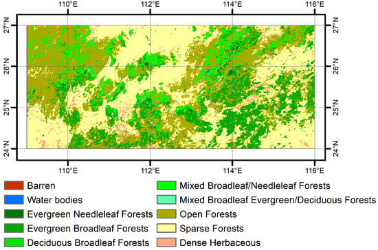
Figure 1.
The MCD12Q1 land cover map for the year 2001 with the FAO-Land Cover Classification System 1 over the Nanling Mountains. The presented map has been resampled to 1 km spatial resolution.
2.2. Datasets
2.2.1. GEOV2 LAI Time Series
We used the 10-day composite GEOV2 LAI time series at 1 km spatial resolution (0.008929°) from 1999 to 2019 provided by the Copernicus Global Land Service (https://land.copernicus.vgt.vito.be/PDF/portal/Application.html#Home) (accessed on 17 March 2022). In this product, neural networks algorithm is used to estimate LAI with SPOT/VGT and PROBA-V canopy reflectance as inputs [,]. This product was selected for the estimation of vegetation phenology partially due to that LAI time series can reflect leaf dynamics directly []. Furthermore, the delivered GEOV2 LAI time series product has been smoothed by the producer []. This makes the product easy to use in the Nanling Mountains with frequently cloudy optical satellite observations. The GEOV2 LAI product was reported to show good performance for estimating phenological metrics of maize in northern China [] and forests in Europe [].
2.2.2. Climate Data
We used the ERA5-land monthly precipitation, air temperature at 2 m above the surface, and surface downwards solar radiation during 1999–2019 []. These data were obtained from the Climate Data Store (https://cds.climate.copernicus.eu/cdsapp#!/home) (accessed on 21 March 2022). The spatial resolution of the ERA5-land reanalysis dataset is 0.1°. We resampled the ERA5-land climate data to 1 km using nearest neighbor method.
2.2.3. Land Cover Maps and DEM
The MODIS C6 MCD12Q1 500 m land cover product [] for 2001 was obtained from the NASA land processes Distributed Active Archive Center (LP DAAC) (https://lpdaac.usgs.gov/) (accessed on 10 May 2021). The C6 version uses a random forests algorithm to classify land cover types and takes advantage of land cover information from other resources to adjust class probabilities []. We selected the land cover layer with the FAO-Land Cover Classification System 1 (LCCS1) that contains eight forest types. There are widespread sparse forests (tree cover 10%–30%) over the study area (Figure 1). These forests mainly occur in flat areas and are mostly the mixture of crops and trees. Sparse forests are therefore excluded from analyses. We resampled the MCD12Q1 land cover map to 1 km spatial resolution. This map was finally used to identify forest types for the analyses of the spatio-temporal variation in SOS.
For open forests with a fractional tree cover of 30%–60% at 1 km spatial resolution, there can also exist a mixture of forests and croplands. Here, we used the 30 m GLC_FCS30 land cover map in 2015 [] provided at zenodo (https://zenodo.org/record/3986872#.YqBVYuhByUm) (accessed on 29 April 2022) to detect mixed pixels. The land-cover classification system of this map provides both rainfed and irrigated croplands that may show distinct phenological circles in this subtropical region.
We obtained the 30 m NASADEM product, a refined version of DEM produced by NASA [], from https://search.earthdata.nasa.gov/search (accessed on 23 March 2022).
2.3. Estimation of SOS
The GEOV2 LAI product provides smoothed and gap filled 10-day interval time series, while there are remaining noises that may lead to uncertainties in SOS estimation. We applied the adaptive Savitzky–Golay filtering provided in the TIMESAT 3.3 software [,,] to further smooth the LAI time series. We selected the STL replace method to remove spikes and outliers and to assign weights of the remaining points with a STL stiffness value of 3.0 in the TIMESAT 3.3 software. Furthermore, the window size of the Savitzky–Golay filtering was 6. Many studies used a threshold-based method to estimate the SOS [,,,]. Using GEOV1 LAI data, Verger et al. reported that a 30% LAI threshold matched the budburst of B. pendula better than other thresholds []. Here, the SOS was estimated using a 30% LAI seasonal amplitude.
2.4. Statistical Analyses
2.4.1. Spatial Variation in SOS
We compared differences in multiyear mean SOS along latitude and elevation gradients. The latitude was divided into three bins because of the small latitude extent of the Nanling Mountains (3°). The elevational gradient of multiyear mean SOS may be heterogeneous across the Nanling mountains, which show strong spatial differences in the local climate []. Therefore, we used spatial moving windows to characterize the SOS elevation gradients at a local scale [], with a window size of 51 × 51 pixels (approximately 51 × 51 km) and a step length of 10 pixels. The elevation gradients were not calculated for moving windows with less than 1300 forested pixels (half of the total pixels of a moving window).
For coarse spatial resolution satellite observations, a complex landscape pattern can lead to many mixed pixels with different vegetation types. Hence, spatial variations in satellite-observed vegetation phenology may be related to both climate differences and mixed pixels [,,]. We selected two subregions to investigate the impacts of mixed pixels on the observed SOS elevation gradients.
2.4.2. Temporal Variation in SOS and Its Response to Climate Factors
Monotonic trends in the SOS over 1999–2019 were characterized using ordinary least square linear regression. We computed the Spearman rank partial correlation coefficients between interannual variations in SOS and preseason climate factors (mean air temperature, total precipitation, and total surface radiation) by pixels. We used climate data from January to April according to the multiyear mean SOS across the region (Section 3.1). Previous studies have shown spatially varying preseasons for modelling vegetation phenology–climate relationships [,]. Here, we considered three lengths of preseason, including one, two and three months. We also calculated the sensitivity of SOS to preseason air temperature by using multiple linear regression []. Furthermore, when performing the partial correlation analysis and multiple linear regression, we used the detrended time series of SOS and preseason climate factors, i.e., the residuals of the linear regression of time series against time, as inputs to reduce possible bias [].
3. Results
3.1. Spatial Pattern of SOS across the Nanling Mountains
The forests across the Nanling Mountains showed a large SOS range with the 5% and 95% percentiles of the multiyear mean SOS of DOY 81.7 and 105.8, respectively. The spatial pattern of SOS was heterogeneous, with many areas showing sharp spatial variation in SOS (Figure 2a). We revealed a slightly earlier regional mean SOS in the southern region (24–25° N) than those in the central and northern regions (Figure 2c).
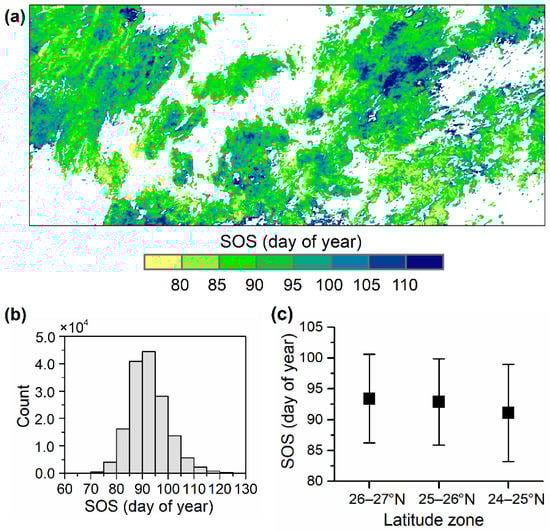
Figure 2.
Spatial pattern of the start of the growing season (SOS) over the Nanling Mountains. (a) Spatial distribution of the multiyear mean SOS for the period of 1999–2019, (b) the frequency distribution of the multiyear mean SOS, and (c) the regional mean SOS and the standard deviation for each latitude zone.
As expected, the spatial distribution of the elevation gradients of the SOS calculated using spatial moving windows was heterogeneous (Figure 3). Positive SOS elevation gradients accounted for only 52.7% of the moving windows. Furthermore, only 99 (6.9%) moving windows showed elevation gradients greater than 10 days/1000 m. These moving windows were mainly distributed in the center of the region.
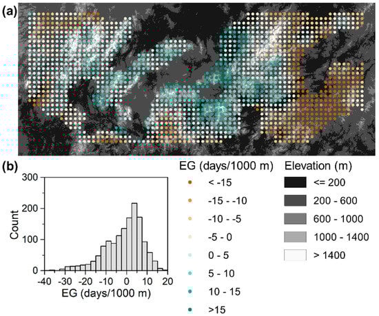
Figure 3.
Elevation gradients (EG) of the multiyear mean SOS across the region. (a) Spatial pattern of the SOS elevation gradients. The points represent the centers of the spatial moving windows, and (b) the frequency distribution of the SOS elevation gradients.
An overlay of SOS later than DOY 102 (90% percentile) with DEM suggests that pixels with a later SOS were mostly (75%) located at elevations lower than 661 m (Figure 4), which directly results in the widespread negative SOS elevation gradients. We selected two subregions that contain spatial clusters of later SOS (SOS > 102) at lower elevations to further explain the spatial pattern of SOS. We found pixels with SOS > 102 were mostly a mixture of forests and rainfed croplands, as shown in the GLC_FCS30 land cover map (Figure 4c). This suggests the considerable impacts of mixed pixels at lower elevations on coarse resolution satellite-observed SOS elevational patterns.
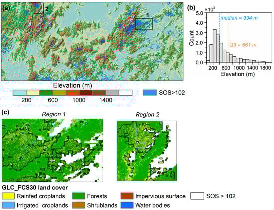
Figure 4.
(a) Spatial distribution of pixels with SOS later than day of year 102 (90% percentile). (b) The histogram shows the elevations of these pixels. Q3 represents the 75% percentile of the elevation values. (c) Two selected regions containing mixed pixels of forests and croplands with SOS > 102.
3.2. Temporal Variation in SOS from 1999 to 2019
The interannual profile of the regional mean SOS is provided in Figure 5. For the forests across the entire Nanling Mountains, SOS showed a slope of −0.20 days/year (p = 0.21) during 1999–2019. Figure 6 displays the spatial patterns of changes in SOS. A strong spatial clustering of SOS change was observed. Pixels with trends toward earlier SOS mainly distributed in the northern region, while later trend in SOS generally occurred in the southern region. In the northwestern region, many pixels exhibited SOS advance by more than 1.0 days/year. In total, approximately 22% of the analyzed forested pixels over the Nanling Mountains experienced significantly earlier trend in the SOS (p < 0.1, Table 1). Percentage of significantly later SOS trend was much smaller. In terms of forest types, mixed forests had the largest percentage of significant trend toward an earlier SOS (39.6%). Furthermore, very few significantly later SOS trend was observed for mixed forests. For evergreen broadleaf forests, only about 11% of the SOS experienced a significantly earlier trend.
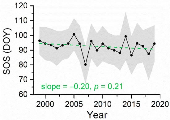
Figure 5.
Interannual variation in the regional mean SOS from 1999 to 2019. The grey band represents one standard deviation of the SOS.
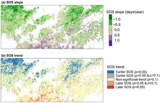
Figure 6.
Spatial patterns of SOS slope (a) and trend (b) during 1999–2019 over the Nanling Mountains.

Table 1.
Proportions of SOS trends for different forest types. EBF, evergreen broadleaf forests; MF, mixed forests; OF, open forests.
3.3. Responses of SOS to Interannual Variations in Climate Factors
The correlations between SOS and the climate factors are presented in Table 2. Of the nine selected preseasons, Spearman partial correlation analysis revealed more negative correlations between SOS and mean air temperature than positive correlations in six preseasons. The largest proportion of significantly negative correlation (p < 0.1) was observed in February–March (37.7%), followed by February (36.2%). These suggest that a warmer spring can advance the SOS in this subtropical region. In contrast to February–March, more positive correlations were observed for January, April, and March–April. Note that for preseasons containing April, only pixels with an SOS later than DOY 100 (10 April) were considered. The proportions of positive correlations between the total precipitation and SOS were greater than those of negative correlations for most preseasons. The largest proportion was 20.2% in March. In addition, impacts of radiation on SOS were generally weak. These results suggest an overall stronger impact of preseason air temperature on SOS than those of the other two climate factors for subtropical forests over the Nanling Mountains.
Table 2.
Statistics of the Spearman partial correlation coefficients between interannual variations in SOS and climate factors at different preseason lengths. For the climate factors, MT represents mean air temperature; TP, total precipitation; TR, total radiation. In the statistical metrics column, %P and %N represent the percentages of positive and negative correlations (p < 0.1), respectively. For the preseasons, the abbreviations are the first letters of months. For example, JFM represents January–February–March.
We further computed statistics on the Spearman partial correlation coefficients between SOS and mean air temperature for different forest types (Table 3). What stands out is the proportions of significantly negative correlations between SOS and air temperature for mixed forests: 58.2% in February–March and 46.9% in February. For the other two forest types, we observed less significantly negative correlations, while the largest proportions were both greater than 30%. Figure 7a displays the spatial distribution of the Spearman partial correlation coefficient between SOS and mean air temperature in February–March (TFM). Stronger negative Spearman’s r was mostly observed in the central region. Sensitivity of SOS to TFM calculated by multiple linear regression was provided in Figure 7b. Although evergreen broadleaf forests showed the overall weakest correlation between SOS and TFM, the SOS sensitivity to TFM was not the weakest. Furthermore, the range of sensitivity to TFM in evergreen broadleaf forests was greatest among the three forest types. The 5% percentiles of the sensitivity to TFM in evergreen broadleaf forests and mixed forests were −5.4 days/°C and −4.8 days/°C, respectively. Many pixels with a sensitivity stronger than −5.0 days/°C can be found in evergreen broadleaf forests in the eastern region.
Table 3.
Statistics of the Spearman partial correlation coefficients between SOS and mean air temperature for different forest types. EBF, evergreen broadleaf forests; MF, mixed forests; OF, open forests.
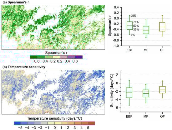
Figure 7.
Relationship between SOS and mean air temperature in February-March (TFM). (a) Spearman partial correlation coefficient (Spearman’s r) by controlling total precipitation and radiation. (b) Sensitivity of SOS to TFM computed by a multiple linear regression. EBF, evergreen broadleaf forests; MF, mixed forests; OF, open forests.
4. Discussion
4.1. Spatial Pattern of SOS
SOS in the Nanling Mountains exhibited a slightly latitude difference with earlier SOS in the southern region (Figure 2). This is generally consistent with the air temperature gradient of the region []. We observed a complex pattern of the elevation gradients of SOS with only about half of the moving windows showing positive gradients. Furthermore, a small proportion of the spatial windows were characterized as elevation gradients greater than 10 days/1000 m. Many studies revealed much greater elevation gradients of spring vegetation phenology in other regions (e.g., [,,]). Although those studies used different datasets and definitions of spring phenology, some showed elevation gradients greater than 20 days/1000 m, such as the Alps [] and the Tianshan Mountains []. Qiu et al. revealed an overall SOS elevation gradient of 14.45 days/1000 m in Fujian province, China, which is adjacent to the Nanling mountains []. For the Xiangjiang river basin located in the northern and central of the Nanling Mountains, Peng et al. reported a SOS elevation gradient of 15.1 days /1000 m for the elevation range of 480–1800 m []. The elevation gradients of SOS at the Xiangjiang river basin shown in Figure 3 generally agreed with that in [].
The large proportion of negative SOS elevation gradients can be partially attributed to the mixed pixel effect of coarse resolution satellite observations (Figure 4c). Open forests at lower elevations generally have higher probability of mixed pixels of forests and croplands, which can lead to later SOS than that of closed forests in higher elevations. On the other hand, Gao et al. also observed many negative SOS elevation gradients in the Northern Hemisphere using the AVHRR GIMMS3g NDVI dataset []. They found that a warming temperature in higher elevations can explain the negative SOS elevation gradients in northeast North America []. The SOS elevation gradients were also likely to be related to the combined impacts of air temperature and precipitation [,]. Further research on the role of climate in the negative SOS elevation gradients is needed for the Nanling Mountains.
4.2. Temporal Variation in SOS and the Responses to Climate Factors
A significantly earlier trend in the SOS (p < 0.1) was observed for approximately 22% of the analyzed forested pixels over the Nanling Mountains. Only about 5% of the pixels showed a significant delay in the SOS. Earlier trends in spring phenology over this subtropical region were also observed in [], which estimated the spring phenological metric using solar-induced chlorophyll fluorescence data during 2002–2017. Yuan et al. observed a regional average SOS change slope of −0.448 days/year during 1982–2015 covering a northern part of the Nanling Mountains []. In [], SOS was extracted from the GIMMS3g NDVI time series using a 20% relative threshold. Furthermore, croplands were not excluded from that analysis []. Ma and Zhou reported earlier trend in SOS during 1980–2006 over subtropical forests in China based on multiple datasets []. Although these studies are with different spatio-temporal extents, they indicate that advance in spring phenology across the subtropical Nanling Mountains was observable in recent decades.
At a regional scale, the preseason air temperature was found to have generally stronger impacts on the SOS than the other two climate factors (Table 2). These results were generally in line with those of previous studies on subtropical vegetation in southern China [,,]. Furthermore, mixed forests showed the strongest response to spring air temperature among the three major forest types (Table 3). This may be explained by the generally higher proportion of deciduous trees in mixed forests than that in evergreen forests []. Likewise, a stronger relationship between spring photosynthetic phenology and air temperature was observed in mixed forests than in evergreen forests across southern China [].
Another finding was that the negative correlation between SOS and air temperature was stronger from February to March for all forest types (Table 2 and Table 3). The air temperature in other analyzed months exhibited much weaker impacts on SOS. This indicates that the direct influence of spring warming on leaf development was limited to one or two months for the subtropical forests in the Nanling Mountains. Li et al. reported a large range of preseason length of air temperature across southern China with many lengths longer than 90 days [], while in the Nanling Mountains, the preseason seems much shorter. It should be noted that we used monthly climate data, and the preseason length can be further refined. Yuan et al. reported that the response of SOS to air temperature was stronger to a 16-day preseason length than 30 and 60 days in a small part of the Nanling Mountains []. In addition, we noted some proportions around 10% for a positive correlation between SOS and air temperature in January for evergreen broadleaf forests and open forests (Table 2 and Table 3). A possible explanation for this may be that a higher winter temperature may result in lack of winter chilling []. Previous studies have reported neglected and complicated influences of winter chilling on spring leaf phenology of subtropical trees based on ground observations [] and controlled experiments [].
4.3. Limitations
The spatio-temporal pattern of SOS across the Nanling Mountains was characterized by using the GEOV2 LAI time series at a 1 km spatial resolution. We have showed the impacts of mixed pixels on the elevational pattern of the SOS in this mountainous region with a complex landscape pattern (Figure 4). Phenological metrics estimated from satellite data with multiple spatial resolutions are required for a better interpretation of the spatial variation in the SOS in this region [,]. Mixed pixels can also cause uncertainties in the statistical responses of vegetation dynamics to climate factors [,,], as different species generally show diverse responses to climate factors [,]. In other words, there should be uncertainties in the statistical relationships between SOS and climate factors for some open forests due to mixed pixels. Further understanding of spring leaf phenology may benefit from systematic evaluation of the impacts of mixed pixel on satellite-observed SOS and the climate drivers across this subtropical mountainous region [,]. On the other hand, we focused on the general responses of the SOS to the preseason mean air temperature; the role of winter chilling in SOS variations requires further investigation for this region.
5. Conclusions
This study set out to characterize the spatio-temporal variation in satellite-observed SOS for subtropical forests across the Nanling Mountains in southern China. The major findings are described below.
(1) A complex spatial pattern of SOS with spatially varying and many negative elevation gradients were observed. Mixed pixels in open forests at lower elevations, particularly mixture of forests and rainfed croplands, could partially explain this.
(2) Approximately 22% of the subtropical forests experienced a significantly earlier SOS (p < 0.1). In general, interannual variation in SOS was found to be controlled more by the spring air temperature (February to March) than by precipitation and radiation, as well as the air temperature in winter. Furthermore, mixed forests containing deciduous trees showed the strongest response to air temperature variation. These findings enhance the understanding of the climate drivers of spring leaf phenology of subtropical forests in a mountainous environment.
Author Contributions
Conceptualization, C.D.; methodology, C.D. and W.H.; software, B.Z.; formal analysis, C.D. and Y.M.; investigation, C.D.; writing—original draft preparation, C.D.; writing—review and editing, W.H., Y.M. and B.Z.; funding acquisition, C.D. and W.H. All authors have read and agreed to the published version of the manuscript.
Funding
This study was funded by the Strategic Priority Research Program of Chinese Academy of Sciences (Grant No. XDA26010304), the National Natural Science Foundation of China (Grant No. 42071320), and a grant from Beijing Normal University (Grant No. 310432101).
Data Availability Statement
Publicly available datasets were analyzed in this study. The websites for accessing the datasets are provided within the article.
Acknowledgments
We thank the anonymous reviewers for their constructive comments on the manuscript.
Conflicts of Interest
The authors declare no conflict of interest. The funders had no role in the design of the study; in the collection, analyses, or interpretation of data; in the writing of the manuscript; or in the decision to publish the results.
References
- Grêt-Regamey, A.; Brunner, S.H.; Kienast, F. Mountain Ecosystem Services: Who Cares? Mt. Res. Dev. 2012, 32, S23–S34. [Google Scholar] [CrossRef]
- Pepin, N.C.; Arnone, E.; Gobiet, A.; Haslinger, K.; Kotlarski, S.; Notarnicola, C.; Palazzi, E.; Seibert, P.; Serafin, S.; Schöner, W.; et al. Climate Changes and Their Elevational Patterns in the Mountains of the World. Rev. Geophys. 2022, 60, e2020RG000730. [Google Scholar] [CrossRef]
- Asse, D.; Chuine, I.; Vitasse, Y.; Yoccoz, N.G.; Delpierre, N.; Badeau, V.; Delestrade, A.; Randin, C.F. Warmer Winters Reduce the Advance of Tree Spring Phenology Induced by Warmer Springs in the Alps. Agric. For. Meteorol. 2018, 252, 220–230. [Google Scholar] [CrossRef]
- Dunn, A.; de Beurs, K.M. Land Surface Phenology of North American Mountain Environments Using Moderate Resolution Imaging Spectroradiometer Data. Remote Sens. Environ. 2011, 115, 1220–1233. [Google Scholar] [CrossRef]
- Thompson, J.A.; Paull, D.J. Assessing Spatial and Temporal Patterns in Land Surface Phenology for the Australian Alps (2000–2014). Remote Sens. Environ. 2017, 199, 1–13. [Google Scholar] [CrossRef]
- Vitasse, Y.; Signarbieux, C.; Fu, Y.H. Global Warming Leads to More Uniform Spring Phenology across Elevations. Proc. Natl. Acad. Sci. USA 2018, 115, 1004–1008. [Google Scholar] [CrossRef]
- Richardson, A.D.; Keenan, T.F.; Migliavacca, M.; Ryu, Y.; Sonnentag, O.; Toomey, M. Climate Change, Phenology, and Phenological Control of Vegetation Feedbacks to the Climate System. Agric. For. Meteorol. 2013, 169, 156–173. [Google Scholar] [CrossRef]
- Caparros-Santiago, J.A.; Rodriguez-Galiano, V.; Dash, J. Land Surface Phenology as Indicator of Global Terrestrial Ecosystem Dynamics: A Systematic Review. ISPRS J. Photogramm. Remote Sens. 2021, 171, 330–347. [Google Scholar] [CrossRef]
- Beresford, A.E.; Sanderson, F.J.; Donald, P.F.; Burfield, I.J.; Butler, A.; Vickery, J.A.; Buchanan, G.M. Phenology and Climate Change in Africa and the Decline of Afro-Palearctic Migratory Bird Populations. Remote Sens. Ecol. Conserv. 2019, 5, 55–69. [Google Scholar] [CrossRef]
- Oeser, J.; Heurich, M.; Senf, C.; Pflugmacher, D.; Belotti, E.; Kuemmerle, T. Habitat Metrics Based on Multi-Temporal Landsat Imagery for Mapping Large Mammal Habitat. Remote Sens. Ecol. Conserv. 2020, 6, 52–69. [Google Scholar] [CrossRef] [Green Version]
- Huete, A.; Didan, K.; Miura, T.; Rodriguez, E.P.P.; Gao, X.; Ferreira, L.G.G. Overview of the Radiometric and Biophysical Performance of the MODIS Vegetation Indices. Remote Sens. Environ. 2002, 83, 195–213. [Google Scholar] [CrossRef]
- Verger, A.; Filella, I.; Baret, F.; Peñuelas, J. Vegetation Baseline Phenology from Kilometric Global LAI Satellite Products. Remote Sens. Environ. 2016, 178, 1–14. [Google Scholar] [CrossRef]
- Shahgedanova, M.; Adler, C.; Gebrekirstos, A.; Grau, H.R.; Huggel, C.; Marchant, R.; Pepin, N.; Vanacker, V.; Viviroli, D.; Vuille, M. Mountain Observatories: Status and Prospects for Enhancing and Connecting a Global Community. Mt. Res. Dev. 2021, 41, A1–A15. [Google Scholar] [CrossRef]
- Gao, M.; Piao, S.; Chen, A.; Yang, H.; Liu, Q.; Fu, Y.H.; Janssens, I.A. Divergent Changes in the Elevational Gradient of Vegetation Activities over the Last 30 Years. Nat. Commun. 2019, 10, 2970. [Google Scholar] [CrossRef]
- Misra, G.; Asam, S.; Menzel, A. Ground and Satellite Phenology in Alpine Forests Are Becoming More Heterogeneous across Higher Elevations with Warming. Agric. For. Meteorol. 2021, 303, 108383. [Google Scholar] [CrossRef]
- Ding, C.; Huang, W.; Liu, M.; Zhao, S. Change in the Elevational Pattern of Vegetation Greenup Date across the Tianshan Mountains in Central Asia during 2001–2020. Ecol. Indic. 2022, 136, 108684. [Google Scholar] [CrossRef]
- Dai, J.; Zhu, M.; Mao, W.; Liu, R.; Wang, H.; Alatalo, J.M.; Tao, Z.; Ge, Q. Divergent Changes of the Elevational Synchronicity in Vegetation Spring Phenology in North China from 2001 to 2017 in Connection with Variations in Chilling. Int. J. Climatol. 2021, 41, 6109–6121. [Google Scholar] [CrossRef]
- Qiu, B.; Zhong, M.; Tang, Z.; Chen, C. Spatiotemporal Variability of Vegetation Phenology with Reference to Altitude and Climate in the Subtropical Mountain and Hill Region, China. Chin. Sci. Bull. 2013, 58, 2883–2892. [Google Scholar] [CrossRef]
- Qader, S.H.; Atkinson, P.M.; Dash, J. Spatiotemporal Variation in the Terrestrial Vegetation Phenology of Iraq and Its Relation with Elevation. Int. J. Appl. Earth Obs. Geoinf. 2015, 41, 107–117. [Google Scholar] [CrossRef]
- Correa-Díaz, A.; Romero-Sánchez, M.E.; Villanueva-Díaz, J. The Greening Effect Characterized by the Normalized Difference Vegetation Index Was Not Coupled with Phenological Trends and Tree Growth Rates in Eight Protected Mountains of Central Mexico. For. Ecol. Manag. 2021, 496, 119402. [Google Scholar] [CrossRef]
- Tang, Z.; Wang, Z.; Zheng, C.; Fang, J. Biodiversity in China’s Mountains. Front. Ecol. Environ. 2006, 4, 347–352. [Google Scholar] [CrossRef]
- Peng, H.; Xia, H.; Chen, H.; Zhi, P.; Xu, Z. Spatial Variation Characteristics of Vegetation Phenology and Its Influencing Factors in the Subtropical Monsoon Climate Region of Southern China. PLoS ONE 2021, 16, e0250825. [Google Scholar] [CrossRef] [PubMed]
- Zhou, G.; Zhang, H.; Zhou, P. Multi-disciplinary Research Values of the Nanling Mountains. Trop. Geogr. 2018, 38, 293–298. [Google Scholar] [CrossRef]
- Qian, S.; Chen, X.; Lang, W.; Schwartz, M.D. Examining Spring Phenological Responses to Temperature Variations during Different Periods in Subtropical and Tropical China. Int. J. Clim. 2021, 41, 3208–3218. [Google Scholar] [CrossRef]
- Li, X.; Fu, Y.H.; Chen, S.; Xiao, J.; Yin, G.; Li, X.; Zhang, X.; Geng, X.; Wu, Z.; Zhou, X.; et al. Increasing Importance of Precipitation in Spring Phenology with Decreasing Latitudes in Subtropical Forest Area in China. Agric. For. Meteorol. 2021, 304–305, 108427. [Google Scholar] [CrossRef]
- Yuan, M.; Wang, L.; Lin, A.; Liu, Z.; Qu, S. Variations in Land Surface Phenology and Their Response to Climate Change in Yangtze River Basin during 1982–2015. Theor. Appl. Climatol. 2019, 137, 1659–1674. [Google Scholar] [CrossRef]
- Zhu, B.; Chen, A.; Liu, Z.; Fang, J. Plant community composition and tree species diversity on eastern and western Nanling Mountains, China. Biodivers. Sci. 2004, 12, 53–62. [Google Scholar]
- Wang, Y.; Dong, Y. Geographical Detection of Regional Demarcation in the Nanling Mountains. Trop. Geogr. 2018, 38, 337–346. [Google Scholar] [CrossRef]
- Verger, A.; Baret, F.; Weiss, M. GEOV2/VGT: Near real time estimation of global biophysical variables from VEGETATION-P data. In Proceedings of the MultiTemp 2013: 7th International Workshop on the Analysis of Multi-temporal Remote Sensing Images, Banff, AB, Canada, 25–27 June 2013; pp. 1–4. [Google Scholar] [CrossRef]
- Verger, A.; Camacho, F.; Van der Goten, R.; Jacobs, T. Product User Manual: LAI, FAPAR, Fcover Collection 1 km Version 2. 2019. Available online: https://land.copernicus.eu/global/sites/cgls.vito.be/files/products/CGLOPS1_PUM_LAI1km-V2_I1.33.pdf (accessed on 29 March 2022).
- Yu, H.; Yin, G.; Liu, G.; Ye, Y.; Qu, Y.; Xu, B.; Verger, A. Validation of Sentinel-2, MODIS, CGLS, SAF, GLASS and C3S Leaf Area Index Products in Maize Crops. Remote Sens. 2021, 13, 4529. [Google Scholar] [CrossRef]
- Muñoz-Sabater, J.; Dutra, E.; Agustí-Panareda, A.; Albergel, C.; Arduini, G.; Balsamo, G.; Boussetta, S.; Choulga, M.; Harrigan, S.; Hersbach, H.; et al. ERA5-Land: A State-of-the-Art Global Reanalysis Dataset for Land Applications. Earth Syst. Sci. Data 2021, 13, 4349–4383. [Google Scholar] [CrossRef]
- Friedl, M.; Sulla-Menashe, D. MCD12Q1 MODIS/Terra+Aqua Land Cover Type Yearly L3 Global 500 m SIN Grid V006 [Data Set]; NASA EOSDIS Land Processes DAAC; USGS: Sioux Falls, SD, USA, 2019. [CrossRef]
- Sulla-Menashe, D.; Gray, J.M.; Abercrombie, S.P.; Friedl, M.A. Hierarchical Mapping of Annual Global Land Cover 2001 to Present: The MODIS Collection 6 Land Cover Product. Remote Sens. Environ. 2019, 222, 183–194. [Google Scholar] [CrossRef]
- Liu, L.Y.; Zhang, X.; Chen, X.D.; Gao, Y.; Mi, J. Global Land-Cover Product with Fine Classification System at 30 m Using Time-Series Landsat Imagery (Version v1) [Data Set]. Zenodo. 2020. Available online: https://zenodo.org/record/3986872#.YyHksnZBxBD (accessed on 29 April 2022).
- NASA JPL. NASADEM Merged DEM Global 1 arc Second V001. NASA EOSDIS Land Processes DAAC. 2020. Available online: https://cmr.earthdata.nasa.gov/search/concepts/C1546314043-LPDAAC_ECS.html (accessed on 5 September 2022).
- Jönsson, P.; Eklundh, L. TIMESAT—A Program for Analyzing Time-Series of Satellite Sensor Data. Comput. Geosci. 2004, 30, 833–845. [Google Scholar] [CrossRef]
- Jönsson, P.; Eklundh, L. Seasonality Extraction by Function Fitting to Time-Series of Satellite Sensor Data. IEEE Trans. Geosci. Remote Sens. 2002, 40, 1824–1832. [Google Scholar] [CrossRef]
- Eklundh, L.; Jönsson, P. Timesat 3.3 Software Manual. Lund and Malmö University, Sweden. 2017. Available online: https://web.nateko.lu.se/timesat/timesat.asp?cat=6 (accessed on 30 June 2020).
- Cho, M.A.; Ramoelo, A.; Dziba, L. Response of Land Surface Phenology to Variation in Tree Cover during Green-up and Senescence Periods in the Semi-Arid Savanna of Southern Africa. Remote Sens. 2017, 9, 689. [Google Scholar] [CrossRef]
- Wang, J.; Zhang, X.; Rodman, K. Land Cover Composition, Climate, and Topography Drive Land Surface Phenology in a Recently Burned Landscape: An Application of Machine Learning in Phenological Modeling. Agric. For. Meteorol. 2021, 304–305, 108432. [Google Scholar] [CrossRef]
- Ding, C.; Huang, W.; Zhao, S.; Zhang, B.; Li, Y.; Huang, F.; Meng, Y. Greenup Dates Change across a Temperate Forest-Grassland Ecotone in Northeastern China Driven by Spring Temperature and Tree Cover. Agric. For. Meteorol. 2022, 314, 108780. [Google Scholar] [CrossRef]
- Gong, Y.; Staudhammer, C.L.; Wiesner, S.; Starr, G.; Zhang, Y. Characterizing Growing Season Length of Subtropical Coniferous Forests with a Phenological Model. Forests 2021, 12, 95. [Google Scholar] [CrossRef]
- Shen, M.; Piao, S.; Chen, X.; An, S. Strong Impacts of Daily Minimum Temperature on the Green-up Date and Summer Greenness of the Tibetan Plateau. Glob. Chang. Biol. 2016, 22, 3057–3066. [Google Scholar] [CrossRef]
- Iler, A.M.; Inouye, D.W.; Schmidt, N.M.; Høye, T.T. Detrending Phenological Time Series Improves Climate-Phenology Analyses and Reveals Evidence of Plasticity. Ecology 2017, 98, 647–655. [Google Scholar] [CrossRef] [Green Version]
- Ma, T.; Zhou, C. Climate-Associated Changes in Spring Plant Phenology in China. Int. J. Biometeorol. 2012, 56, 269–275. [Google Scholar] [CrossRef]
- Chen, X.; Wang, L.; Inouye, D. Delayed Response of Spring Phenology to Global Warming in Subtropics and Tropics. Agric. For. Meteorol. 2017, 234–235, 222–235. [Google Scholar] [CrossRef]
- Zhang, R.; Lin, J.; Wang, F.; Shen, S.; Wang, X.; Rao, Y.; Wu, J.; Hänninen, H. The Chilling Requirement of Subtropical Trees Is Fulfilled by High Temperatures: A Generalized Hypothesis for Tree Endodormancy Release and a Method for Testing It. Agric. For. Meteorol. 2021, 298–299, 108296. [Google Scholar] [CrossRef]
- Zhang, X.; Wang, J.; Gao, F.; Liu, Y.; Schaaf, C.; Friedl, M.; Yu, Y.; Jayavelu, S.; Gray, J.; Liu, L.; et al. Exploration of Scaling Effects on Coarse Resolution Land Surface Phenology. Remote Sens. Environ. 2017, 190, 318–330. [Google Scholar] [CrossRef]
- Liu, Y.; McDonough MacKenzie, C.; Primack, R.B.; Hill, M.J.; Zhang, X.; Wang, Z.; Schaaf, C.B. Using Remote Sensing to Monitor the Spring Phenology of Acadia National Park across Elevational Gradients. Ecosphere 2021, 12, e03888. [Google Scholar] [CrossRef]
- Helman, D. Land Surface Phenology: What Do We Really ‘See’ from Space? Sci. Total Environ. 2018, 618, 665–673. [Google Scholar] [CrossRef]
- Jin, J.; Yan, T.; Zhu, Q.; Wang, Y.; Guo, F.; Liu, Y.; Hou, W. Heterogeneity of Land Cover Data with Discrete Classes Obscured Remotely-Sensed Detection of Sensitivity of Forest Photosynthesis to Climate. Int. J. Appl. Earth Obs. Geoinf. 2021, 104, 102567. [Google Scholar] [CrossRef]
- Park, D.S.; Newman, E.A.; Breckheimer, I.K. Scale Gaps in Landscape Phenology: Challenges and Opportunities. Trends Ecol. Evol. 2021, 36, 709–721. [Google Scholar] [CrossRef]
- Richardson, A.D.; O’Keefe, J. Phenological Differences Between Understory and Overstory. In Phenology of Ecosystem Processes; Noormets, A., Ed.; Springer: New York, NY, USA, 2009. [Google Scholar] [CrossRef]
- Fang, Z.; Brandt, M.; Wang, L.; Fensholt, R. A Global Increase in Tree Cover Extends the Growing Season Length as Observed from Satellite Records. Sci. Total Environ. 2022, 806, 151205. [Google Scholar] [CrossRef]
Publisher’s Note: MDPI stays neutral with regard to jurisdictional claims in published maps and institutional affiliations. |
© 2022 by the authors. Licensee MDPI, Basel, Switzerland. This article is an open access article distributed under the terms and conditions of the Creative Commons Attribution (CC BY) license (https://creativecommons.org/licenses/by/4.0/).