Abstract
Coastal wetlands provide the unique biogeochemical functions of storing a large fraction of the terrestrial carbon (C) pool and being among the most productive ecosystems in the world. However, coastal wetlands face numerous natural and anthropogenic disturbances that threaten their ecological integrity and C storage potential. To monitor the C balance of a coastal forested wetland, we established an eddy covariance flux tower in a natural undrained bottomland hardwood forest in eastern North Carolina, USA. We examined the long-term trends (2009–2019) in gross primary productivity (GPP), ecosystem respiration (RE), and the net ecosystem C exchange (NEE) seasonally and inter-annually. We analyzed the response of C fluxes and balance to climatic and hydrologic forcings and examined the possible effects of rising sea levels on the inland groundwater dynamics. Our results show that in 2009, a higher annual GPP (1922 g C m−2 yr−1) was observed than annual RE (1554 g C m−2 yr−1), resulting in a net C sink (NEE = −368 g C m−2 yr−1). However, the annual C balance switched to a net C source in 2010 and onwards, varying from 87 g C m−2 yr−1 to 759 g C m−2 yr−1. The multiple effects of air temperature (Tair), net radiation (Rn), groundwater table (GWT) depth, and precipitation (p) explained 66%, 71%, and 29% of the variation in GPP, RE, and NEE, respectively (p < 0.0001). The lowering of GWT (−0.01 cm to −14.26 cm) enhanced GPP and RE by 35% and 28%, respectively. We also observed a significant positive correlation between mean sea level and GWT (R2 = 0.11), but not between GWT and p (R2 = 0.02). Cumulative fluxes from 2009 to 2019 showed continuing C losses owing to a higher rate of increase of RE than GPP. This study contributes to carbon balance accounting to improve ecosystem models, relating C dynamics to temporal trends in under-represented coastal forested wetlands.
1. Introduction
Coastal wetlands serve important functions, such as providing food and bio-materials as direct resources, acting as wildlife sanctuaries, storing a large fraction of the terrestrial carbon (C) pool, protecting against storm surges, and facilitating sediment accumulation for land accretion [1,2,3]. They also provide water purification, tourism resorts, and other functionalities [1], and are considered among the most productive and economically valuable ecosystems in the world [4]. They occupy 4%–6% of Earth’s land area and store approximately 202–535 Gt of C [5], with 0.031 to 0.034 Gt of wetland C stored in the USA [6]. Along the coastal plain of the southeastern USA, wetlands play a significant role in regulating regional ecohydrology [4,7] and in the productivity of economically important crops, timber, and fishery resources [8]. The importance of coastal forested wetlands in providing a range of ecosystem services and their role in aboveground-and-belowground C storage is well-recognized. However, deeper understanding of the net C balance of coastal forested wetlands has not been well-explored [2,3,9,10,11,12,13].
Coastal wetlands face numerous natural and anthropogenic disturbances that threaten their ecological integrity and C storage potential. These threats include land-use change [7,9], climate change [12,13,14,15,16,17,18], and sea-level rise (SLR) [19,20,21,22,23,24,25,26,27], leading to the problems of saltwater intrusion [7,28,29] and prolonged inundation [30,31,32]. With climate change, SLR is expected to attain between +0.4 m and +1.2 m relative to today by the year 2100 [15,33,34], accompanied by a higher frequency and intensity of coastal storms [35,36]. These coastal phenomena are already resulting in ‘ghost forest’ formation due to the prolonged inundation and submergence of low-lying land [21,28,37]. Thus, studies to understand the short-term and long-term impact of these disturbances are needed to assess the forest C budget temporal patterns and future trajectories.
Carbon fluxes, such as gross primary productivity (GPP) and ecosystem respiration (RE), and the corresponding net ecosystem exchange (NEE), are strongly influenced by climate [38,39,40,41,42,43]. Light, atmospheric temperature, and water availability mainly control C fluxes [39,40,44,45,46,47]. Years with high rainfall amounts result in less sunlight, which may reduce GPP [41] while dryer years are associated with more sunlight, which may increase GPP; however, it may also result in greater deficits in soil moisture, causing stomatal closure, hence reducing GPP [48,49]. On the other hand, RE increases exponentially with temperature, given sufficient soil moisture, yet declines if soils are too dry or wet [50,51]. Understanding the influence of climatic drivers on the forest C balance is important because the climate–C cycle feedbacks control landscape C balances in response to climate warming [45,52,53], yet studies that examine these effects remain limited [40].
Therefore, to monitor the long-term net C balance of a coastal forested wetland, we established an eddy covariance flux tower within a natural undrained bottomland hardwood forest in eastern North Carolina, USA. We examined the long-term trends (2009–2017) in gross primary production (GPP), ecosystem respiration (RE), and net ecosystem C exchange (NEE), seasonally and inter-annually. We analyzed the response of C fluxes and balance to climatic and hydrologic forcings, and examined the possible effect of rising sea levels on the inland groundwater dynamics. This study contributes to carbon accounting using a more accurate approach to improve ecosystem models relating C dynamics to temporal trends in wetland ecosystems.
2. Materials and Methods
2.1. The Study Site
The area of study is within the Alligator River National Wildlife Refuge (ARNWR), Dare County, North Carolina, USA, specifically at 35°45′16.44″ N and 75°54′13.64″ (Figure 1). The eddy covariance flux tower is coded as US-NC4 in the FLUXNET registry. FLUXNET is a global network of micrometeorological tower sites that monitor the land—atmosphere exchange of carbon, water vapor, and energy fluxes. The US-NC4 flux tower was established in 2009. The tower stands within a >100-year-old natural coastal bottomland hardwood forest with natural drainage. Historically the site was used for timber production, and much of the surrounding area is farmland [54].
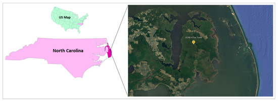
Figure 1.
Location of the eddy covariance flux tower established at the Alligator River National Wildlife Refuge. (ARNWR), Dare Country, North Carlina, USA. Map taken from Google Earth version 9.166.0.1 (accessed on 25 May 2022).
The refuge stretches across more than 154,000 acres of wetland. It is home to various wildlife (e.g., black bears, deer, etc.) and plant species (e.g., Nyssa sylvatica, Nyssa biflora, Taxodium distichum, Liquidambar styraciflua, and Pinus serotina). This wetland forest is also characterized by ‘hummocks’ around tree bases that are usually above the water table and non-vegetated low-lying ‘hollows’ submerged for more than 70% of the year [55]. The soil has 0.3–1.0 m thick organic soil horizons (Oi, Oe, and Oa), belonging to the soil type haplosaprist of the Pungo series (poorly drained with highly decomposed muck and less decomposed peat by highly reduced mineral sediments). The site lies < 1 m above sea level. The average annual rainfall was 1163 mm (1981–2017), and the average temperature was 15.72 °C (2005–2017). More descriptions of the site can be found in [9,44,55,56].
2.2. Ecosystem Flux Measurement
An open-path infrared gas analyzer was used to measure the turbulent fluxes of CO2 exchange consisting of an LI-7500 (LI-COR, Lincoln, NE, USA), a Gill WindMaster sonic anemometer (R-350; Gill Instruments, Lymington, UK), and a CR1000 data logger, mounted at the top of the 32-m high tower (Fetch = ~2500 m).
Micrometerological instruments were used to measure air temperature (HHMP45AC, Vaisala, Finland), photosynthetically active radiation (PAR, LI-190, LI-COR Inc.), net radiation (CNR-1, Kipp & Zonen, Delft, the Netherlands), and precipitation (TE-525, Campbell Scientific Inc., Logan, UT, USA). Below the tower, soil temperature was measured (5 cm and 20 cm depth) using CS107 temperature probes (CSI, Logan, UT, USA). A CS616 time domain reflectometry probe (CSI, Logan, UT, USA) measured the soil volumetric water content. The groundwater table (GWT) was also determined using an ultrasonic water level datalogger (Infinities, Port Orange, FL, USA). The GWT data in 2017 was removed due to instrument malfunction.
2.3. Flux Data Processing and Gap-Filling
We calculated the net ecosystem exchange (NEE) for each 30-min period using the Eddypro software version 6.1.0 (LI-COR Inc., Lincoln, NE, USA). We used the standard quality checks and corrections for the following: spike detection [57], planar fit coordinate rotation of wind vectors [58], time lag corrections, and air density fluctuation [59], and high [60] and low pass filtering [61]. Flux outputs were flagged as 0 (high quality), 1 (medium), and 2 (low quality) when deviations in steady state and integral turbulence characteristics are <30%, >30% to <100%, and >100%, respectively [62].
During the post-processing of the 30-min data, we filtered the data for low signal strength, integral turbulence characteristics, despiking, and low friction velocity [63]. Missing NEE30-min were gap-filled following the Max Planck Institute of Biogeochemistry method in Germany, which is an online protocol ReddyProc: Eddy covariance data processing tool (https://www.bgcjena.mpg.de/bgi/index.php/Services/REddyProcWeb) accessed on 20 February 2022. This web tool automatically partitioned the 30-min NEE into 30-min gross primary production (GPP) and ecosystem respiration (RE). The few remaining gaps (2%–6%) left after gap-filling and flux partitioning using ReddyProc [64] were filled by means of linear interpolation from the corresponding NEE values of the previous and succeeding years. Finally, daily NEE was computed as the sum of NEE30min values over a 24-h period. Monthly averages were also obtained. The seasonality includes winter (January–March), spring (April–June), summer (July–September), and fall (October–December). The growing season usually occurs from April to October, while the non-growing season covers November to March. We present the annual C balance in atmospheric sign convention where positive NEE values connote C loss by the ecosystem, and negative values correspond to C gain [50].
2.4. Mortality and Leaf Area Index Determination
The mortality rates were determined from the 13 circular 7-m radius vegetation monitoring plots established within the flux tower footprint. Within each plot, tree species were identified and individual trees with diameter at breast height (i.e., 1.4 m aboveground level) greater than 2.5 cm were tagged. Diameter at breast height were measured each winter season. Dead trees were also recorded. The leaf area index (LAI) from 2009 to 2019 was generated using the Global Land Surface Satellite (GLASS) LAI datasets [65] from the Moderate Resolution Imaging Spectroradiometer (MODIS) surface reflectance data at an 8-day and 1-km resolution.
2.5. Data Analysis
We performed a generalized additive modeling using the gam function from the mgcv and MuMin packages to predict the best climate drivers of variations in C fluxes and balance [66]. In order to avoid over-parameterization, we used the second-order Akaike information criterion (AIC) in order to determine the best smoothing dimension with an upper limit equal to 3 [67]. The spline term effects were ranked according to their F-values (Wald Tests) [39]. The uncertainties in the C fluxes were obtained using the Monte Carlo bootstrapping approach. The Monte Carlo simulation was used to estimate a “probability” and the bootstrap approach was used to generate the same size of data from the same distribution many times (1000 times in this study). The bootstrap approach treated the original data as the population and was sampled with replacement from that data. The bootstrap function was used on this analysis [68]. Linear relationships were carried out using the ggplot2 [69], ggpubr, plotly [70], tidyverse [71], and reshape [72] packages. The confidence intervals of C fluxes were determined following [73] for the NEE and Monte Carlo approach using the bootstrap package used for GPP and RE. All analyses were processed in R version 4.1.1 [74].
3. Results
3.1. Seasonal and Interannual Variations in Major Climate
Global radiation (Rg) and air temperature (Tair) followed a distinct seasonal trend of increasing after the winter season (March) or as the growing season started in spring (April), peaking in mid-summer (mid-July to mid-August) and gradually declining towards the non-growing season (November) (Figure 2). However, groundwater table depth (GWT) and precipitation (p) had no apparent seasonality. The site was intermittently flooded in some periods of the year (mostly during non-growing seasons, max GWT = 24.18 cm), but frequently was also a little drier, mainly during the growing season (min GWT = −14.26) (Figure 2). Inter-annual variation in Rn was small, varying from an annual average of 90.20 W m−2 in 2009 to 126.96 W m−2 in 2017. Inter-annual variation in average yearly air temperature only varied from 15.56 °C in 2014 to 17.89 °C in 2012. The annual average GWT from 2010 to 2013 was low (−4.35 cm to −0.03 cm). However, the site was submerged most of the time from 2014 to 2019, with an annual average GWT of 0.22 cm to 6.91 cm above the soil surface.
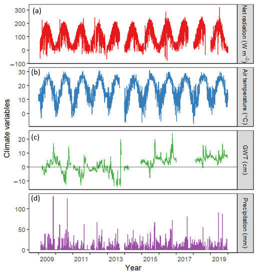
Figure 2.
Seasonal variations in (a) net radiation (Rn), (b) air temperature (Tair), (c) groundwater table depth (GWT), and (d) precipitation. Daily data from 2009–2019 obtained from the eddy covariance flux tower in Alligator River National Wildlife Refuge, Dare County, North Carolina, USA was used.
3.2. Seasonal and Inter-Annual Variation in Carbon Fluxes and Balance
Across all years, the seasonal variation in GPP and RE were distinct. An increasing GPP and RE were apparent from the end of the non-growing season in winter towards spring. However, GPP and RE peaked in summer and gradually declined towards fall (Figure 3). Average daily GPP and RE during the growing season were 8.09 g C m−2 d−1 and 8.31 g C m−2 d−1, respectively. During the non-growing season, the average GPP was 2.25 g C m−2 d−1, and RE was 3.04 g C m−2 d−1. However, the seasonal variation in net ecosystem exchange was less distinct (Figure 3). During the growing season, NEE showed lower C loss (0.21 g C m−2 d−1) when the vegetation was active than during the non-growing season (0.79 g C m−2 d−1). Thus, photosynthesis and respiration during the growing season were higher than during the non-growing seasons, when GPP and RE were low (Figure 3, p < 0.05). This pattern was fairly consistent across the study duration, except for anomalous spikes in 2010 and 2011, which we attribute to either flux system performance or random measurement errors.
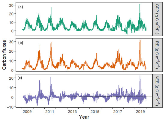
Figure 3.
Seasonal variation in (a) gross primary productivity (GPP), (b) ecosystem respiration (RE), and (c) net ecosystem exchange (NEE) from 2009–2019. Daily data were obtained from the eddy covariance flux tower (US-NC4) in Alligator River National Wildlife Refuge, Dare County, North Carolina, USA.
In 2009, a higher annual GPP than the annual RE was observed (Table 1). This higher GPP than RE resulted in a net C sink. However, the annual carbon balance switched to a net C source from 2010 onwards, when RE continued to exceed GPP. The weak C source varied largely from 87 g C m−2 yr−1 in 2010 to as high as 759 g C m−2 yr−1 in 2017 (Table 1). We found a 27% inter-annual variation in GPP while that of RE was 36%.

Table 1.
Annual gross primary production (GPP), ecosystem respiration (RE), and net ecosystem exchange (NEE) from 2009 to 2019. The upper and lower limits were determined using the uncertainty analysis of [57] for NEE, while Monte Carlo (bootstrap) simulation was used for GPP and RE.
3.3. Climatic Effects on Carbon Fluxes and Balance
The combined effects of Tair, Rn, GWT, and p explained 66%, 71%, and 29% of the variation in GPP, RE, and NEE, respectively (p < 0.0001, Table 2). Among the key climatic variables, the best fit models revealed Tair to be the main driver of GPP (F value = 119.29, p < 0.0001), RE (255.13, p < 0.0001), and NEE (42.31, p < 0.0001) (Table 2). It was observed that water level fluctuations better explained GPP and RE than the radiation component, whereas p explained the least in the GPP, RE, and NEE models (Table 2).
Table 2.
Results of generalized additive modeling (GAM) analysis to detect the best models and rank predictor variables e.g., air temperature (Tair), net radiation (Rn), groundwater table depth (GWT), and Precipitation (p) according to their ability to explain variation in gross primary productivity (GPP), ecosystem respiration (RE), and net ecosystem exchange (NEE). Daily data from 2009–2019 were used in the analysis. In order to avoid model over-parameterization, the second-order Akaike information criterion was used to determine the best smoothing dimension with an upper limit equal to 3. We report the coefficient of the fitted model with values for each spline term in turn.
Since the variation in Tair and Rn remained relatively constant across years, we focus on GWT variation in the succeeding sections, as it was the most varied among the climate variables. It was also the second best predictor variable for GPP and RE (Figure 2; Table 2). We evaluated how GWT was driving the carbon fluxes, especially RE, considering the prolonged inundation characteristic of the site, where tree mortality is accelerating.
When GWT levels were below the soil surface (GWT = −0.01 cm to −14.26 cm), GPP and RE were enhanced by 35% and 28%, respectively (Figure 4). When GWT was taken as a sole predictor for GPP and RE alone, negative correlations were observed between GWT and GPP (R2 = 0.19) and GWT and RE (R2 = 0.20) during the growing season. However, the relationships between GWT with that of GPP and RE were weak during the non-growing season, with R2 = 0.05 and R2 = 0.02 for GPP and RE, respectively. (Figure 4). GWT had low explanatory power for the dynamics in NEE in both the growing and non-growing seasons.
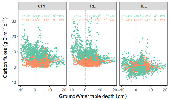
Figure 4.
Linear relationships between groundwater table depth (GWT) and gross primary productivity (GPP), ecosystem respiration (RE), and net ecosystem exchange (NEE) during the growing (green circles and equations) and non-growing seasons (orange circles and equations) from 2009–2019. Daily data was used in the analysis.
3.4. Groundwater Level and the Rising Sea Level
GWT and mean sea level both increased over time, especially from 2015 onwards (Figure 5a), with a weak statistical relationship (R2 = 0.11; Figure 5b). It is worth noting that the flux tower is approximately 20 km away from the coastline, which explains the weak relationship between GWT and mean sea level. We also observed a positive correlation between seawater level during tidal cycles and GWT (figure not shown). The relationship between GWT and sea level during low tide was higher (R2 = 0.32) than during high tide (R2 = 0.19).
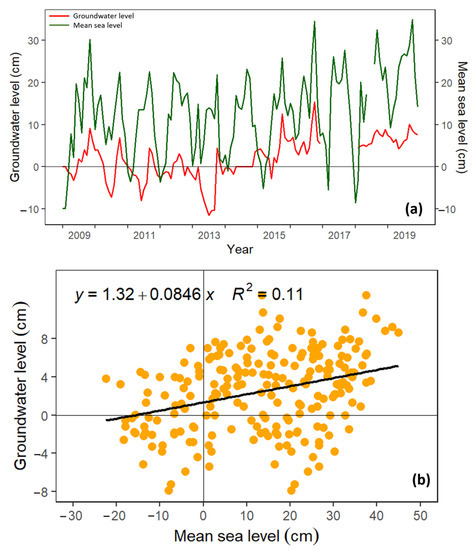
Figure 5.
Panel (a) is the time series of groundwater table depth (GWT) and mean sea level using monthly data from 2009–2019, while panel (b) is the linear relationship between GWT and mean sea level.
3.5. The Cumulative Trends of Carbon Fluxes and Balance
A higher daily cumulative RE than GPP (p < 0.05) over the years of observation caused the ecosystem to be a net C emitter (Figure 6).
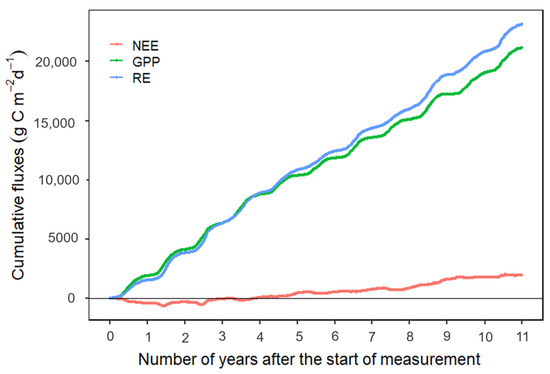
Figure 6.
Cumulative gross primary productivity (GPP), ecosystem respiration (RE), and net ecosystem exchange (NEE) for 2009–2019 from flux monitoring of a coastal forested wetland at the Alligator River Natural Wildlife Refuge in Dare County, North Carolina, USA.
4. Discussion
4.1. Sources of Uncertainties
The eddy covariance measurement methodology is subject to uncertainties due to systematic errors [75] or random errors [76] that are difficult to assess. Despite the gap-filling methods developed for flux uncertainty, problems still exist [63,77,78]. Although these gap-filling errors affect the magnitude of the fluxes, all seasons and years should be affected similarly, allowing us to make comparisons over time.
In addition, our LAI is derived from remote-sensing data products. We caution the readers on using satellite-based LAI, as this approach may underestimate or overestimate LAI [79,80,81]. These uncertainties may occur due to overlapping or clumping between leaves and light obstruction from branches, boles, and stems [82].
4.2. Seasonal and Inter-Annual Variation in C Fluxes and Balance
The seasonal trends of NEE reflect the different phases and amplitudes in GPP and RE [83]. The largest carbon uptake occurred during the peak of the growing season (July–August) when irradiance was high, and temperature was at its peak. We observed a high GPP during the growing season, when greater solar radiation and high temperatures induced canopy development and high assimilation rates. This result is consistent with other studies [9,10,84,85,86,87].
Nine years of monitoring the C balance of a natural coastal forested wetland along the southeastern US revealed how the ecosystem has transitioned from a net carbon sink during the measurement in 2009 into a net carbon source (2010–2017). Many old-growth forests have a decadal average of NEE close to zero [52] or are carbon sinks [88] unless the ecosystem is disturbed. Our site’s long-term net C source condition may be ascribed to many tree physiological and environmental perturbations. These may include tree mortality, declining productivity, and thus LAI, prolonged hydroperiod, SLR, and saltwater intrusion, among others that are highly intertwined. We tackle each factor below with supporting data, except for saltwater intrusion and the construction of ditches, for which we based our explanations on previous work.
4.2.1. Effect of Tree Mortality on Carbon Fluxes
The decline in the annual rate of GPP compared to RE resulted in the ecosystem becoming a net carbon source over the years. A net loss of C to the atmosphere is likely due to the “drowning” of vegetation, causing increased tree mortality. Currently, there are hundreds of dead trees and stumps at ARNWR that were once part of a thriving wetland forest and are now part of a ghost forest. Ghost forests are made up of the remnants of the dead but still-standing trees. These trees are limbless and no longer have a leaf canopy or a functioning vascular system. We found only one dead tree per hectare a year after the start of measurements in 2009, yet that figure rose to 17 dead trees per hectare at the end of 2019 (Figure 7). Dead tree biomass may contribute up to 61% of all coarse woody debris on the forest floor [89], ultimately contributing to higher RE [90]. An increase of the number of dead trees on the forest floor indicates a major transformation of the ecosystem. This high incidence of mortality suggests that the environmental controls over NEE have slowly transitioned, resulting in the ecosystem losing stored C. A previous study from nearby the study site also reported 67% overstory mortality [27] and attributed this forest vegetation decline to increasing inundation. Over time, this increasing tree mortality leads to less canopy cover and shifts in species composition of the ecosystem.
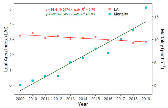
Figure 7.
The linear relationship between leaf area index (LAI) and mortality with annual time series, using the annual averages from 2009–2019.
4.2.2. Declining Leaf Area Index
LAI is a key driver of GPP [44]. In our study, inter-annual change in LAI was less variable, only ranging from 2.95 to 3.42. It must be noted that our wetland forest is a mature > 100-year-old ecosystem, and accordingly, LAI gradually stabilized with increasing age [91]. However, the significant reduction in LAI (R2 = 0.70, Figure 7) from 2009–2019 suggests a decline in forest productivity over the years, thus turning the forest into a net carbon source.
4.2.3. Effect of Prolonged Hydroperiod on Carbon Fluxes
Relative to inundation, our site experienced a prolonged hydroperiod from 2009–2017, especially during the non-growing season (Figure 2). Extreme hydrological conditions alter wetland functioning [32]. High water level affects oxygen availability, soil organic matter decomposition rates, nutrient mobilization [85,92], and plant productivity [86,93]. During flooding, anaerobic respiration within the roots of plants produces toxic byproducts and limits the uptake of nutrients and water. Despite adaptations of some wetland trees to withstand inundation anoxia, constant flooding will cause stress since anaerobic conditions can only persist in the rooting zone for a few weeks during the growing season [94]. Flooding also triggers seedlings’ mortality, limiting the population density, and thus, productivity. Also, plant litter decomposition generally responds quickly to changes in environmental conditions [95,96]. Litter decomposition may contribute most to respiration when the flooding subsides due to soil aeration and extracellular enzymatic activities of soil microorganisms. Prolonged flooding also affects seed germination and seedling recruitment [97]. Plants succumb to hydrological stress when it exceeds the tolerance limits of even flood-tolerant species. The continuing mortality at our site may lead to ecosystem transition from the mixed bottomland hardwood forest into a shrub-dominated pocosin with continued hydrologic stress, as is being seen in other parts of the Refuge [9,27].
4.2.4. Potential Impacts of Sea Level Rise
Projections reveal a future sea level ranging from +0.4 m to +1.2 m relative to today by 2100 [15,35]. Our analysis revealed that as SLR increases, the groundwater level around the study site is also increasing (Figure 5). This increase of SLR indirectly decreased gross primary productivity and enhanced ecosystem respiration (Figure 4) through its effects on GWT, gradually shifting the forest towards a net positive carbon ecosystem exchange. This condition means that the forest will remain a net carbon source unless mitigated. Along with changes in carbon fluxes, we can expect to see a decrease of species richness and an overall decline in ecosystem diversity [21,28].
Rising sea levels might have impeded site drainage, lengthening the inundation period, and thus, tree mortality. This hydrologic stress might also be the reason for the small annual tree diameter growth and top die-back observed at our site. A previous record at the site from 2009–2019 for species such as bald cypress, red bay, water tupelo, and red maple showed a diameter increase of only 0.17 cm to 0.77 cm from 2009–2019 [9]. This phenomenon is not surprising since other wetland sites in Florida [98] and tidal wetlands in Louisiana [99] also observed this diameter growth suppression. Thus, continued monitoring is needed to examine the physiological problems of trees with prolonged inundation due to SLR.
4.2.5. Potential Impact of Saltwater Intrusion
In addition to hydrologic stress, saltwater intrusion may be a driving factor in the formation of ghost forests [28]. SLR may also increase saltwater intrusion into freshwater ecosystems [7,100], leading to species shifts and landward migration, and thus, to the loss of wetland areas [13,101]. Ghost forests result from exposure to the high salinity of water [28]. As saltwater seeps in, live trees first suffer from reduced annual growth. This manifests as a distressful condition, leading to death. As this continues, new seedling recruitment ceases [102,103]. Although we did not measure salinity exposure regimes in this study, the species at our site are vulnerable to salinity stress [97], and therefore, salinity needs to be monitored moving forward to disentangle the effects of salinity from hydrology. Casual spot measurements have never detected salinity at this relatively inland site, so we suspect the majority of the stress causing tree mortality and declining productivity is due to hydrology, but this is a hypothesis that is still in need of rigorous testing.
4.3. Major Climatic Effects on C Fluxes and Balance
The effect of solar irradiance, atmospheric air temperature, and soil water availability on GPP, RE, and NEE has been widely reported [39,40,87,104,105,106]. It is important to determine the influence of these key climate drivers on forest C cycling because the climate–C cycle feedbacks control ecosystem-level C dynamics in response to the changing climate [45,52,53]. However, a deeper understanding of these climate effects on C balance remains limited, especially for coastal forested wetlands.
The combined effect of climatic drivers (Tair, Rn, GWT, and p) only explained 29% of the variability in NEE, suggesting greater biological control (e.g., LAI, mortality, etc.) on NEE than the climate drivers. Determining the response of carbon fluxes and balance to climate and vegetative factors is essential to understand the mechanisms behind the variations in GPP, RE, and NEE. However, obtaining biological data is more challenging than obtaining the climate variables [107]. Previous studies showed that biological effects could be larger [107,108], equivalent to [109], or less than [107,108] climatic effects at an interannual scale. Other studies also studied the correlations between climatic and biological effects [107,109], reflecting the responses of ecosystem C cycling to the changing climate.
Sustained favorable light availability resulting in increased GPP is well established in many studies [39,87,105,110] and is primarily a function of higher LAI [80,90]. However, at our site, GPP, RE, and NEE were not mainly controlled by net radiation but rather by temperature. This result suggests that, in this coastal wetland setting, caution must be taken in using solar irradiance to model C balance as other biological and environmental factors may contribute to the observed variability.
Air temperature is the major climatic control for RE for many studies [56,111,112]. Increased temperature enhanced litter decomposition in areas with abundant water [110,113,114,115,116,117,118]. The sensitivity of RE to temperature may lead to continuing losses of C to the atmosphere due to hydrologic forcing coupled with a future warmer climate.
Surprisingly, GWT contributed more to the RE variability than Rn (Table 2). The microtopography of our site influences the local hydrologic conditions. The hummocks surrounding tree bases are usually above the water table, while the hollows (usually non-vegetated) are submerged more than 70% of the year [55]. Site conditions such as this do not necessarily improve the GPP and RE. Instead, GPP and RE were enhanced during times of decreased groundwater level. Since NEE is the function of its component GPP and RE, the absence of variation in NEE with GWT suggests that even though GWT secondarily controls the variations in GPP and RE, they converge towards a relatively stable NEE. Therefore, modeling must be cognizant of using GWT to parameterize NEE in this mostly submerged wetland site.
During the non-growing season, the water table at our site is at full storage capacity [44], due to the low topographic setting and distinct microtopography. The site is a basin for the water from the nearby uplands. However, the water is difficult to drain because of the proximity of our site to the sea. The poor drainage characteristic of the site and poorly defined pathways for run-off decreased the overland flow. However, a deeper water table is attained during the growing seasons when precipitation is low. Thus, seasonal change in hydrology must be considered when modeling a unique coastal plain forest such as ours.
4.4. Why Do Changes in Groundwater Level Matter to Carbon Dynamics?
The site has low topographic setting characterized by seasonally dynamic high water levels. The variance explained for the negative linear relationship between GWT and GPP (R2 = 0.19) and RE (R2 = 0.20) appeared to behave similarly. However, a higher RE level (max = 29.78 g C m−2 d−1) than GPP (max = 27.45 g C m−2 d−1) (p > 0.05) when the GWT levels were decreased (GWT = 0 and below) suggests that the change in hydrology is affecting respiratory processes more than photosynthesis.
A previous study at our site reported that during non-flooded periods, 57% of the total ecosystem RE came from heterotrophic respiration, while 43% came from autotrophic respiration [55]. However, the reverse occurred during flooded periods. Autotrophic respiration contributed 69% of the total RE, while 31% came from heterotrophic respiration [55]. With this, we deduced that the greater sensitivity of ecosystem respiration to groundwater table drawdown was due to the higher sensitivity of soil respiration compared to plant respiration. Therefore, any reduction in water level at our site would positively stimulate soil respiration. More investigation is needed to better understand the hydrologic controls over RE in forested wetlands. Nevertheless, our results imply that increased hydrologic forcing and the changing climate could potentially shift the C balance trajectory of regional carbon fluxes and balance.
4.5. Is the Unabated Net C Source Strength in the Wetland Forest a Point of No Return?
Given continuing C losses for a prolonged period of time now (Figure 6), we expect that the formation of “ghost forests” brought about by the constant submergence of low-lying land will continue. Sea levels have risen at an average of 2.1–2.4 mm year−1 during the past two millennia [15,34,117]. Models suggest that coastal wetlands will migrate inland towards the freshwater wetlands, thereby increasing the wetland area up to 60% by the year 2100 for a 1.1 m SLR [21]. Carbon dating of organic sediments at a nearby site shows a historical organic soil accumulation rate of 1.11 to 1.13 mm year−1, which is not enough to keep pace with the recent rise in sea level of 2.1 to 2.4 mm year−1, resulting in ecosystem transition and ghost forest formation [26].
Therefore, a quantitative understanding of the effects of climatic extremes on coastal wetland hydrologic function is a pressing research need to inform wetland forest management. Studies that will determine the causes and consequences of forested coastal wetland ecosystem transitions are necessary to improve our understanding of the future of coastal wetland responses to environmental changes and the estimation of regional terrestrial C fluxes. Leaving this scenario as it is, without intervention, will finally set this ecosystem into a point of no return as the continental margin adjusts to SLR.
4.6. Forest Management Options
The accelerated transformation of wetland areas into ghost forests is alarming. In ARNWR alone, 32% of the refuge (31,600 hectares) has seen a change in land cover over 35 years, where 1151 ha of land is now open ocean, and about 19,200 ha of forest has transitioned to marshland or shrubland [107]. As of 2021, about 11% has transitioned to ghost forest [118].
Thus, wetland management interventions are needed to prevent aboveground carbon loss, whether through land preservation, reforestation, or the introduction of new tolerant species into the wetland environments. However, controversy arises in allowing new salt-tolerant vegetation to thrive and adapt within the wetland forests, as it may fail to preserve the current ecosystem.
What can be done to solve this issue and prevent above-ground carbon loss? While it may be too late to prevent harmful SLR, there are some mitigation strategies that should be used to limit the damage to this important coastal system. The most realistic strategy is to facilitate wetland migration. Essentially, this idea involves ensuring that salt tolerant vegetation is introduced as the ecosystem transitions. This prevents the area from turning into open water, and allows for the continued service of carbon sequestration. Ultimately, the long-term result would be the replacement of the ghost forest with a salt marsh ecosystem. Other strategies that should be explored include freshwater leaching and the engineering of structures that protect against SLR. However, these strategies are likely to be extremely costly, and are far less realistic than facilitated wetland migration. There is also a need for more research on the emergence of ghost forests and coastal forest resilience, particularly in regard to saltwater intrusion and salinity tolerance in these ecosystems. If nothing is done to mitigate this transition, North Carolina’s wetland forest could be left with very little vegetation, decimating the ecosystem.
5. Conclusions
Over 11 years of monitoring C fluxes and balance in coastal forested wetland showed that the site had become a net carbon emitter for an extended period of time. The net C source strength was ascribed to the spike in tree mortality, declining productivity, prolonged hydroperiodicity, SLR, and potentially to saltwater intrusion. This natural wetland forest is highly affected by the hydrologic and climatic forcings that could worsen the future net C source trajectory, transitioning this ecosystem to a point of no return as the coastal margin adjusts to unabated SLR. Thus, various wetland management interventions or facilitative wetland migration plans must be explored to minimize aboveground carbon loss from these important coastal wetland forests in North Carolina.
Author Contributions
Conceptualization, M.A., J.K., A.N. and G.S.; methodology, M.A., G.S. and J.K.; software, I.W., M.I., O.G., S.G., T.P., N.L., B.M., P.P. and L.Y.; validation, M.A., I.W., M.I., O.G., S.G. and T.P.; formal analysis, M.A., I.W., M.I., O.G., S.G. and T.P.; investigation, M.A., F.P., S.B., S.P., M.K., L.Y., A.N., G.S., K.M. and J.K.; resources, G.S., S.M., A.N. and J.K.; data curation, M.A., N.L. and L.Y.; writing—original draft preparation, M.A., I.W., M.I., O.G., S.G. and T.P.; writing—review and editing, M.A., I.W., M.I., O.G., S.G., M.K., T.P, G.S., S.M., N.L. and J.K.; visualization, M.A., I.W., M.I., O.G., S.G. and T.P.; supervision, A.N. and J.K.; project administration, A.N. and J.K.; funding acquisition, A.N. and J.K. All authors have read and agreed to the published version of the manuscript.
Funding
Primary funding was provided by the USDA NIFA (Multi-agency A.5 Carbon Cycle Science Program) award 2014-67003-22068. Additional funding was provided by the DOE NICCR award 08-SC-NICCR-1072, the USDA Forest Service award 13-JV-11330110-081, and the DOE LBNL award DE-AC02-05CH11231.
Data Availability Statement
Not applicable.
Acknowledgments
We are grateful to ARNWR Management for the long-term access to the US-NC4 flux site and others in-kind support. We are also thankful to George Hess and Omoyemeh Ile for their guidance to the students involved in this paper.
Conflicts of Interest
The authors declare no conflict of interest.
References
- Li, X.; Bellerby, R.; Craft, C.; Widney, S.E. Coastal Wetland Loss, Consequences, and Challenges for Restoration. Anthr. Coasts 2018, 15, 1–15. [Google Scholar] [CrossRef]
- Casey, W.P.; Ewel, K.C. Patterns of Succession in Forested Depressional Wetlands in North Florida, USA. Wetlands 2006, 26, 147–160. [Google Scholar] [CrossRef]
- Nahlik, A.M.; Fennessy, M.S. Carbon Storage in US Wetlands. Nat. Commun. 2016, 7, 13835. [Google Scholar] [CrossRef] [PubMed]
- Moreno-Mateos, D.; Power, M.E.; Comín, F.A.; Yockteng, R. Structural and Functional Loss in Restored Wetland Ecosystems. PLoS Biol. 2012, 10, e1001247. [Google Scholar] [CrossRef]
- Mitra, S.; Wassmann, R.; Vlek, P.L.G. An Appraisal of Global Wetland Area and Its Organic Carbon Stock. Curr. Sci. 2005, 88, 25–35. [Google Scholar]
- Derouin, S. Study Finds That Coastal Wetlands Excel at Storing Carbon. Eos 2017, 98, eo069971. [Google Scholar] [CrossRef]
- White, E.; Kaplan, D. Restore or Retreat? Saltwater Intrusion and Water Management in Coastal Wetlands. Ecosyst. Health Sustain. 2017, 3, e01258. [Google Scholar] [CrossRef]
- Bullock, A.; Acreman, M. The Role of Wetlands in the Hydrological Cycle. Hydrol. Earth Syst. Sci. Discuss. 2003, 7, 358–389. [Google Scholar] [CrossRef]
- Aguilos, M.; Mitra, B.; Noormets, A.; Minick, K.; Prajapati, P.; Gavazzi, M.; Sun, G.; McNulty, S.; Li, X.; Domec, J.C.; et al. Long-Term Carbon Flux and Balance in Managed and Natural Coastal Forested Wetlands of the Southeastern USA. Agric. For. Meteorol. 2020, 288–289, 108022. [Google Scholar] [CrossRef]
- Amatya, D.M.; Skaggs, R.W. Hydrologic Modeling of a Drained Pine Plantation on Poorly Drained Soils. For. Sci. 2001, 47, 103–114. [Google Scholar]
- Tor-ngern, P.; Oren, R.; Palmroth, S.; Novick, K.; Oishi, A.; Linder, S.; Ottosson-Löfvenius, M.; Näsholm, T. Water Balance of Pine Forests: Synthesis of New and Published Results. Agric. For. Meteorol. 2018, 259, 107–117. [Google Scholar] [CrossRef]
- Truus, L. Estimation of Above-Ground Biomass of Wetlands. In Biomass and Remote Sensing of Biomass; Institute of Ecology at Tallinn University Estonia: Tallinn, Estonia, 2011. [Google Scholar] [CrossRef]
- Stagg, C.L.; Schoolmaster, D.R.; Piazza, S.C.; Snedden, G.; Steyer, G.D.; Fischenich, C.J.; McComas, R.W. A Landscape-Scale Assessment of Above- and Belowground Primary Production in Coastal Wetlands: Implications for Climate Change-Induced Community Shifts. Estuaries Coasts 2017, 40, 856–879. [Google Scholar] [CrossRef]
- Day, J.W.; Christian, R.R.; Boesch, D.M.; Yáñez-Arancibia, A.; Morris, J.; Twilley, R.R.; Naylor, L.; Schaffner, L.; Stevenson, C. Consequences of Climate Change on the Ecogeomorphology of Coastal Wetlands. Estuaries Coasts 2008, 31, 477–491. [Google Scholar] [CrossRef]
- Horton, B.P.; Rahmstorf, S.; Engelhart, S.E.; Kemp, A.C. Expert Assessment of Sea-Level Rise by AD 2100 and AD 2300. Quat. Sci. Rev. 2014, 84, 1–6. [Google Scholar] [CrossRef]
- Cormier, N.; Krauss, K.W.; Conner, W.H. Periodicity in Stem Growth and Litterfall in Tidal Freshwater Forested Wetlands: Influence of Salinity and Drought on Nitrogen Recycling. Estuaries Coasts 2013, 36, 533–546. [Google Scholar] [CrossRef]
- Ensign, S.H.; Hupp, C.R.; Noe, G.B.; Krauss, K.W.; Stagg, C.L. Sediment Accretion in Tidal Freshwater Forests and Oligohaline Marshes of the Waccamaw and Savannah Rivers, USA. Estuaries Coasts 2014, 37, 1107–1119. [Google Scholar] [CrossRef]
- Sun, G.; Caldwell, P.; Noormets, A.; McNulty, S.G.; Cohen, E.; Moore Myers, J.; Domec, J.-C.; Treasure, E.; Mu, Q.; Xiao, J.; et al. Upscaling Key Ecosystem Functions across the Conterminous United States by a Water-Centric Ecosystem Model. J. Geophys. Res. 2011, 116, G00J05. [Google Scholar] [CrossRef]
- Smart, L.S.; Taillie, P.J.; Poulter, B.; Vukomanovic, J.; Singh, K.K.; Swenson, J.J.; Mitasova, H.; Smith, J.W.; Meentemeyer, R.K. Aboveground Carbon Loss Associated with the Spread of Ghost Forests as Sea Levels Rise. Environ. Res. Lett. 2020, 15, 104028. [Google Scholar] [CrossRef]
- Raabe, E.A.; Stumpf, R.P. Expansion of Tidal Marsh in Response to Sea-Level Rise: Gulf Coast of Florida, USA. Estuaries Coasts 2016, 39, 145–157. [Google Scholar] [CrossRef]
- Schuerch, M.; Spencer, T.; Temmerman, S.; Kirwan, M.L.; Wolff, C.; Lincke, D.; McOwen, C.J.; Pickering, M.D.; Reef, R.; Vafeidis, A.T.; et al. Future Response of Global Coastal Wetlands to Sea-Level Rise. Nature 2018, 561, 231–234. [Google Scholar] [CrossRef]
- Crosby, S.C.; Sax, D.F.; Palmer, M.E.; Booth, H.S.; Deegan, L.A.; Bertness, M.D.; Leslie, H.M. Salt Marsh Persistence Is Threatened by Predicted Sea-Level Rise. Estuar. Coast. Shelf Sci. 2016, 181, 93–99. [Google Scholar] [CrossRef]
- Neumann, B.; Vafeidis, A.T.; Zimmermann, J.; Nicholls, R.J. Future Coastal Population Growth and Exposure to Sea-Level Rise and Coastal Flooding—A Global Assessment. PLoS ONE 2015, 10, e0131375. [Google Scholar] [CrossRef] [PubMed]
- Kirwan, M.L.; Temmerman, S.; Skeehan, E.E.; Guntenspergen, G.R.; Fagherazzi, S. Overestimation of Marsh Vulnerability to Sea Level Rise. Nat. Clim. Chang. 2016, 6, 253–260. [Google Scholar] [CrossRef]
- Bhattachan, A.; Jurjonas, M.D.; Moody, A.C.; Morris, P.R.; Sanchez, G.M.; Smart, L.S.; Taillie, P.J.; Emanuel, R.E.; Seekamp, E.L. Sea Level Rise Impacts on Rural Coastal Social-Ecological Systems and the Implications for Decision Making. Environ. Sci. Policy 2018, 90, 122–134. [Google Scholar] [CrossRef]
- McTigue, N.; Davis, J.; Rodriguez, A.B.; McKee, B.; Atencio, A.; Currin, C. Sea Level Rise Explains Changing Carbon Accumulation Rates in a Salt Marsh Over the Past Two Millennia. J. Geophys. Res. Biogeosci. 2019, 124, 2945–2957. [Google Scholar] [CrossRef]
- Aguilos, M.; Brown, C.; Minick, K.; Fischer, M.; Ile, O.J.; Hardesty, D.; Kerrigan, M.; Noormets, A.; King, J. Millennial-Scale Carbon Storage in Natural Pine Forests of the North Carolina Lower Coastal Plain: Effects of Artificial Drainage in a Time of Rapid Sea Level Rise. Land 2021, 10, 1294. [Google Scholar] [CrossRef]
- Kirwan, M.L.; Gedan, K.B. Sea-Level Driven Land Conversion and the Formation of Ghost Forests. Nat. Clim. Chang. 2019, 9, 450–457. [Google Scholar] [CrossRef]
- Ardón, M.; Morse, J.L.; Colman, B.P.; Bernhardt, E.S. Drought-Induced Saltwater Incursion Leads to Increased Wetland Nitrogen Export. Glob. Chang. Biol. 2013, 19, 2976–2985. [Google Scholar] [CrossRef]
- Aguilos, M.; Sun, G.; Noormets, A.; Domec, J.C.; McNulty, S.; Gavazzi, M.; Prajapati, P.; Minick, K.J.; Mitra, B.; King, J. Ecosystem Productivity and Evapotranspiration Are Tightly Coupled in Loblolly Pine (Pinus taeda L.) Plantations along the Coastal Plain of the Southeastern U.S. Forests 2021, 12, 1123. [Google Scholar] [CrossRef]
- Minick, K.J.; Mitra, B.; Li, X.; Fischer, M.; Aguilos, M.; Prajapati, P.; Noormets, A.; King, J.S. Wetland Microtopography Alters Response of Potential Net CO2 and CH4 Production to Temperature and Moisture: Evidence from a Laboratory Experiment. Geoderma 2021, 402, 115367. [Google Scholar] [CrossRef]
- Ketcheson, S.J.; Price, J.S.; Carey, S.K.; Petrone, R.M.; Mendoza, C.A.; Devito, K.J. Constructing Fen Peatlands in Post-Mining Oil Sands Landscapes: Challenges and Opportunities from a Hydrological Perspective. Earth-Sci. Rev. 2016, 161, 130–139. [Google Scholar] [CrossRef]
- Holmquist, J.R.; Windham-Myers, L.; Bliss, N.; Crooks, S.; Morris, J.T.; Megonigal, J.P.; Troxler, T.; Weller, D.; Callaway, J.; Drexler, J.; et al. Accuracy and Precision of Tidal Wetland Soil Carbon Mapping in the Conterminous United States. Sci. Rep. 2018, 8, 9478. [Google Scholar] [CrossRef] [PubMed]
- Kemp, A.C.; Kegel, J.J.; Culver, S.J.; Barber, D.C.; Mallinson, D.J.; Leorri, E.; Bernhardt, C.E.; Cahill, N.; Riggs, S.R.; Woodson, A.L.; et al. Extended Late Holocene Relative Sea-Level Histories for North Carolina, USA. Quat. Sci. Rev. 2017, 160, 13–30. [Google Scholar] [CrossRef]
- Rasmussen, D.J.; Bittermann, K.; Buchanan, M.K.; Kulp, S.; Strauss, B.H.; Kopp, R.E.; Oppenheimer, M. Extreme Sea Level Implications of 1.5 °C, 2.0 °C, and 2.5 °C Temperature Stabilization Targets in the 21st and 22nd Centuries. Environ. Res. Lett. 2018, 13, 034040. [Google Scholar] [CrossRef]
- Fickert, T. To Plant or Not to Plant, That Is the Question: Reforestation vs. Natural Regeneration of Hurricane-Disturbed Mangrove Forests in Guanaja (Honduras). Forests 2020, 11, 1068. [Google Scholar] [CrossRef]
- Kirwan, M.L.; Guntenspergen, G.R. Response of Plant Productivity to Experimental Flooding in a Stable and a Submerging Marsh. Ecosystems 2015, 18, 903–913. [Google Scholar] [CrossRef]
- Brümmer, C.; Black, T.A.; Jassal, R.S.; Grant, N.J.; Spittlehouse, D.L.; Chen, B.; Nesic, Z.; Amiro, B.D.; Arain, M.A.; Barr, A.G.; et al. How Climate and Vegetation Type Influence Evapotranspiration and Water Use Efficiency in Canadian Forest, Peatland and Grassland Ecosystems. Agric. For. Meteorol. 2012, 153, 14–30. [Google Scholar] [CrossRef]
- Aguilos, M.; Hérault, B.; Burban, B.; Wagner, F.; Bonal, D. What Drives Long-Term Variations in Carbon Flux and Balance in a Tropical Rainforest in French Guiana? Agric. For. Meteorol. 2018, 253–254, 114–123. [Google Scholar] [CrossRef]
- Barr, A.G.; Black, T.A.; Hogg, E.H.; Griffis, T.J.; Morgenstern, K.; Kljun, N.; Theede, A.; Nesic, Z. Climatic Controls on the Carbon and Water Balances of a Boreal Aspen Forest, 1994–2003. Glob. Chang. Biol. 2007, 13, 561–576. [Google Scholar] [CrossRef]
- Zeri, M.; Sá, L.D.A.; Manzi, A.O.; Araú, A.C.; Aguiar, R.G.; von Randow, C.; Sampaio, G.; Cardoso, F.L.; Nobre, C.A. Variability of Carbon and Water Fluxes Following Climate Extremes over a Tropical Forest in Southwestern Amazonia. PLoS ONE 2014, 9, e88130. [Google Scholar] [CrossRef]
- Von Buttlar, J.; Zscheischler, J.; Rammig, A.; Sippel, S.; Reichstein, M.; Knohl, A.; Jung, M.; Menzer, O.; Arain, M.A.; Buchmann, N.; et al. Impacts of Droughts and Extreme Temperature Events on Gross Primary Production and Ecosystem Respiration: A Systematic Assessment across Ecosystems and Climate Zones. Biogeosciences 2018, 15, 1293–1318. [Google Scholar] [CrossRef]
- Novick, K.A.; Ficklin, D.L.; Stoy, P.C.; Williams, C.A.; Bohrer, G.; Oishi, A.C.; Papuga, S.A.; Blanken, P.D.; Noormets, A.; Sulman, B.N.; et al. The Increasing Importance of Atmospheric Demand for Ecosystem Water and Carbon Fluxes. Nat. Clim. Chang. 2016, 6, 1023–1027. [Google Scholar] [CrossRef]
- Aguilos, M.; Sun, G.; Noormets, A.; Domec, J.C.; McNulty, S.; Gavazzi, M.; Minick, K.; Mitra, B.; Prajapati, P.; Yang, Y.; et al. Effects of Land-Use Change and Drought on Decadal Evapotranspiration and Water Balance of Natural and Managed Forested Wetlands along the Southeastern US Lower Coastal Plain. Agric. For. Meteorol. 2021, 303, 108381. [Google Scholar] [CrossRef]
- Aguilos, M.; Takagi, K.; Liang, N.; Ueyama, M.; Fukuzawa, K.; Nomura, M.; Kishida, O.; Fukazawa, T.; Takahashi, H.; Kotsuka, C.; et al. Dynamics of Ecosystem Carbon Balance Recovering from a Clear-Cutting in a Cool-Temperate Forest. Agric. For. Meteorol. 2014, 197, 26–39. [Google Scholar] [CrossRef]
- Aguilos, M.; Stahl, C.; Burban, B.; Hérault, B.; Courtois, E.; Coste, S.; Wagner, F.; Ziegler, C.; Takagi, K.; Bonal, D. Interannual and Seasonal Variations in Ecosystem Transpiration and Water Use Efficiency in a Tropical Rainforest. Forests 2018, 10, 14. [Google Scholar] [CrossRef]
- Reichstein, M.; Papale, D.; Valentini, R.; Aubinet, M.; Bernhofer, C.; Knohl, A.; Laurila, T.; Lindroth, A.; Moors, E.; Pilegaard, K.; et al. Determinants of Terrestrial Ecosystem Carbon Balance Inferred from European Eddy Covariance Flux Sites. Geophys. Res. Lett. 2007, 34, 1–5. [Google Scholar] [CrossRef]
- Reichstein, M.; Ciais, P.; Papale, D.; Valentini, R.; Running, S.; Viovy, N.; Cramer, W.; Granier, A.; Ogée, J.; Allard, V.; et al. Reduction of Ecosystem Productivity and Respiration during the European Summer 2003 Climate Anomaly: A Joint Flux Tower, Remote Sensing and Modelling Analysis. Glob. Change Biol. 2007, 13, 634–651. [Google Scholar] [CrossRef]
- Wolf, S.; Keenan, T.F.; Fisher, J.B.; Baldocchi, D.D.; Desai, A.R.; Richardson, A.D.; Scott, R.L.; Law, B.E.; Litvak, M.E.; Brunsell, N.A.; et al. Warm Spring Reduced Carbon Cycle Impact of the 2012 US Summer Drought. Proc. Natl. Acad. Sci. USA 2016, 113, 5880–5885. [Google Scholar] [CrossRef]
- Baldocchi, D. “Breathing” of the Terrestrial Biosphere: Lessons Learned from a Global Network of Carbon Dioxide Flux Measurement Systems. Aust. J. Bot. 2008, 56, 1–26. [Google Scholar] [CrossRef]
- Baldocchi, D.; Chu, H.; Reichstein, M. Inter-Annual Variability of Net and Gross Ecosystem Carbon Fluxes: A Review. Agric. For. Meteorol. 2018, 249, 520–533. [Google Scholar] [CrossRef]
- Dunn, A.L.; Barford, C.C.; Wofsy, S.C.; Goulden, M.L.; Daube, B.C. A Long-Term Record of Carbon Exchange in a Boreal Black Spruce Forest: Means, Responses to Interannual Variability, and Decadal Trends. Glob. Change Biol. 2007, 13, 577–590. [Google Scholar] [CrossRef]
- Urbanski, S.; Barford, C.; Wofsy, S.; Kucharik, C.; Pyle, E.; Budney, J.; McKain, K.; Fitzjarrald, D.; Czikowsky, M.; Munger, J.W. Factors Controlling CO2 Exchange on Timescales from Hourly to Decadal at Harvard Forest. J. Geophys. Res. Biogeosci. 2007, 112, G02020. [Google Scholar] [CrossRef]
- Mossotti, T. Alligator River National Wildlife Refuge. Ecotone 2013, 8, 86–87. [Google Scholar] [CrossRef]
- Miao, G.; Noormets, A.; Domec, J.C.; Fuentes, M.; Trettin, C.C.; Sun, G.; McNulty, S.G.; King, J.S. Hydrology and Microtopography Control Carbon Dynamics in Wetlands: Implications in Partitioning Ecosystem Respiration in a Coastal Plain Forested Wetland. Agric. For. Meteorol. 2017, 247, 343–355. [Google Scholar] [CrossRef]
- Noormets, A.; Mcnulty, S.G.; Domec, J.C.; Gavazzi, M.; Sun, G.; King, J.S. The Role of Harvest Residue in Rotation Cycle Carbon Balance in Loblolly Pine Plantations. Respiration Partitioning Approach. Glob. Change Biol. 2012, 18, 3186–3201. [Google Scholar] [CrossRef]
- Vickers, D.; Mahrt, L. Quality Control and Flux Sampling Problems for Tower and Aircraft Data. J. Atmos. Ocean Technol. 1997, 14, 512–526. [Google Scholar] [CrossRef]
- Wilczak, J.M.; Oncley, S.P.; Stage, S.A. Sonic Anemometer Tilt Correction Algoriths. Bound.-Layer Meteorol. 2001, 99, 127–150. [Google Scholar] [CrossRef]
- Webb, K.; Pearman, G.I.; Leuning, R. Correction of Flux Measurements for Density Effects Due to Heat and Water Vapour Transfer. Q. J. R. Meteorol. Soc. 1980, 106, 85–100. [Google Scholar] [CrossRef]
- Ibrom, A.; Dellwik, E.; Flyvbjerg, H.; Jensen, N.O.; Pilegaard, K. Strong Low-Pass Filtering Effects on Water Vapour Flux Measurements with Closed-Path Eddy Correlation Systems. Agric. For. Meteorol. 2007, 147, 140–156. [Google Scholar] [CrossRef]
- Moncrieff, J.; Clement, R.; Finnigan, J.; Meyers, T. Averaging, Detrending, and Filtering of Eddy Covariance Time Series. In Handbook of Micrometeorology: A Guide for Surfarce Flux Measurement; Lee, X., Massman, W., Law, B., Eds.; Springer: Dordrecht, The Netherlands, 2004; ISBN 1402022654. [Google Scholar]
- Mauder, T.; Foken, T. Impact of Post-Field Data Processing on Eddy Covariance Flux Estimates and Energy Balance Closure. Meteorol. Z. 2006, 15, 597–609. [Google Scholar] [CrossRef]
- Papale, D.; Reichstein, M.; Aubinet, M.; Canfora, E.; Bernhofer, C.; Kutsch, W.; Longdoz, B.; Rambal, S.; Valentini, R.; Vesala, T.; et al. Towards a Standardized Processing of Net Ecosystem Exchange Measured with Eddy Covariance Technique: Algorithms and Uncertainty Estimation. Biogeosciences 2006, 3, 571–583. [Google Scholar] [CrossRef]
- Wutzler, T.; Lucas-Moffat, A.; Migliavacca, M.; Knauer, J.; Sickel, K.; Šigut, L.; Menzer, O.; Reichstein, M. Basic and Extensible Post-Processing of Eddy Covariance Flux Data with REddyProc. Biogeosciences 2018, 15, 5015–5030. [Google Scholar] [CrossRef]
- Baret, F.; Weiss, M.; Lacaze, R.; Camacho, F.; Makhmara, H.; Pacholcyzk, P.; Smets, B. GEOV1: LAI and FAPAR Essential Climate Variables and FCOVER Global Time Series Capitalizing over Existing Products. Part 1: Principles of Development and Production. Remote Sens. Environ. 2013, 137, 299–309. [Google Scholar] [CrossRef]
- Barton, K. Package ‘ MuMIn ’ Version 1.46.0; R Package. 2022. Available online: https://cran.r-project.org/web/packages/MuMIn/MuMIn.pdf (accessed on 6 June 2022).
- Burnham, K.P.; Anderson, D.R.; Huyvaert, K.P. AIC Model Selection and Multimodel Inference in Behavioral Ecology: Some Background, Observations, and Comparisons. Behav. Ecol. Sociobiol. 2011, 65, 23–35. [Google Scholar] [CrossRef]
- Leisch, F. Functions For the Book “An Introduction to the Bootstrap” Package ‘Bootstrap’. 2019, pp. 1–28. Available online: https://cran.r-project.org/web/packages/bootstrap/bootstrap.pdf (accessed on 6 June 2022).
- Wickham, H. Ggplot2: Elegant Graphics for Data Analysis; Springer: New York, NY, USA, 2016; ISBN 978-3-319-24277-4. [Google Scholar]
- Sievert, C. Interactive Web-Based Data Visualization with R, Plotly, and Shiny; Chapman and Hall/CRC: Boca Raton, FL, USA, 2020; ISBN 9781138331457. [Google Scholar]
- Wickham, H.; Averick, M.; Bryan, J.; Chang, W.; McGowan, L.; François, R.; Grolemund, G.; Hayes, A.; Henry, L.; Hester, J.; et al. Welcome to the Tidyverse. J. Open Source Softw. 2019, 4, 1686. [Google Scholar] [CrossRef]
- Wickham, H. Reshaping Data with the Reshape Package. J. Stat. Softw. 2007, 12, 1–20. [Google Scholar]
- Noormets, A.; Gavazzi, M.J.; McNulty, S.G.; Domec, J.C.; Sun, G.; King, J.S.; Chen, J. Response of Carbon Fluxes to Drought in a Coastal Plain Loblolly Pine Forest. Glob. Change Biol. 2010, 16, 272–287. [Google Scholar] [CrossRef]
- R Core Team. R: A Language and Environment for Statistical Computing; R Core Team: Vienna, Austria, 2021. [Google Scholar]
- Gu, L.; Falge, E.M.; Boden, T.; Baldocchi, D.D.; Black, T.A.; Saleska, S.R.; Suni, T.; Verma, S.B.; Vesala, T.; Wofsy, S.C.; et al. Objective Threshold Determination for Nighttime Eddy Flux Filtering. Agric. For. Meteorol. 2005, 128, 179–197. [Google Scholar] [CrossRef]
- Hollinger, D.Y.; Richardson, A.D. Uncertainty in Eddy Covariance Measurements and Its Implication to Physiological Models. Tree Physiol. 2005, 25, 873–885. [Google Scholar] [CrossRef]
- Moffat, A.M.; Papale, D.; Reichstein, M.; Hollinger, D.Y.; Richardson, A.D.; Barr, A.G.; Beckstein, C.; Braswell, B.H.; Churkina, G.; Desai, A.R.; et al. Comprehensive Comparison of Gap-Filling Techniques for Eddy Covariance Net Carbon Fluxes. Agric. For. Meteorol. 2007, 147, 209–232. [Google Scholar] [CrossRef]
- Soloway, A.D.; Amiro, B.D.; Dunn, A.L.; Wofsy, S.C. Carbon Neutral or a Sink? Uncertainty Caused by Gap-Filling Long-Term Flux Measurements for an Old-Growth Boreal Black Spruce Forest. Agric. For. Meteorol. 2017, 233, 110–121. [Google Scholar] [CrossRef]
- Albaugh, J.M.; Albaugh, T.J.; Heiderman, R.R.; Leggett, Z.; Stape, J.L.; King, K.; O’Neill, K.P.; King, J.S. Evaluating Changes in Switchgrass Physiology, Biomass, and Light-Use Efficiency under Artificial Shade to Estimate Yields If Intercropped with Pinus taeda L. Agrofor. Syst. 2014, 88, 489–503. [Google Scholar] [CrossRef]
- Arias, D.; Calvo-Alvarado, J.; Dohrenbusch, A. Calibration of LAI-2000 to Estimate Leaf Area Index (LAI) and Assessment of Its Relationship with Stand Productivity in Six Native and Introduced Tree Species in Costa Rica. For. Ecol. Manag. 2007, 247, 185–193. [Google Scholar] [CrossRef]
- Liu, Z.; Shao, Q.; Liu, J. The Performances of MODIS-GPP and -ET Products in China and Their Sensitivity to Input Data (FPAR/LAI). Remote Sens. 2015, 7, 135–152. [Google Scholar] [CrossRef]
- Zheng, G.; Moskal, L.M. Retrieving Leaf Area Index (LAI) Using Remote Sensing: Theories, Methods and Sensors. Sensors 2009, 9, 2719–2745. [Google Scholar] [CrossRef]
- Hirano, T.; Segah, H.; Harada, T.; Limin, S.; June, T.; Hirata, R.; Osaki, M. Carbon Dioxide Balance of a Tropical Peat Swamp Forest in Kalimantan, Indonesia. Glob. Change Biol. 2007, 13, 412–425. [Google Scholar] [CrossRef]
- Sarneel, J.M.; Geurts, J.J.M.; Beltman, B.; Lamers, L.P.M.; Nijzink, M.M.; Soons, M.B.; Verhoeven, J.T.A. The Effect of Nutrient Enrichment of Either the Bank or the Surface Water on Shoreline Vegetation and Decomposition. Ecosystems 2010, 13, 1275–1286. [Google Scholar] [CrossRef][Green Version]
- Lamers, L.P.M.; van Diggelen, J.M.H.; Op Den Camp, H.J.M.; Visser, E.J.W.; Lucassen, E.C.H.E.T.; Vile, M.A.; Jetten, M.S.M.; Smolders, A.J.P.; Roelofs, J.G.M. Microbial Transformations of Nitrogen, Sulfur, and Iron Dictate Vegetation Composition in Wetlands: A Review. Front. Microbiol. 2012, 3, 156. [Google Scholar] [CrossRef]
- Wagner, F.; Hérault, B.; Stahl, C.; Bonal, D.; Rossi, V. Modeling Water Availability for Trees in Tropical Forests. Agric. For. Meteorol. 2011, 151, 1202–1213. [Google Scholar] [CrossRef]
- Marcolla, B.; Cescatti, A.; Manca, G.; Zorer, R.; Cavagna, M.; Fiora, A.; Gianelle, D.; Rodeghiero, M.; Sottocornola, M.; Zampedri, R. Climatic Controls and Ecosystem Responses Drive the Inter-Annual Variability of the Net Ecosystem Exchange of an Alpine Meadow. Agric. For. Meteorol. 2011, 151, 1233–1243. [Google Scholar] [CrossRef]
- Luyssaert, S.; Schulze, E.D.; Börner, A.; Knohl, A.; Hessenmöller, D.; Law, B.E.; Ciais, P.; Grace, J. Old-Growth Forests as Global Carbon Sinks. Nature 2008, 455, 213–215. [Google Scholar] [CrossRef] [PubMed]
- Harmon, M.E.; Woodall, C.W.; Fasth, B.; Sexton, J.; Yatkov, M. Differences Between Differences Between Standing and Downed Standing and Downed Dead Tree Wood Density Dead Tree Wood Density Reduction Factors: Reduction Factors: A Comparison Across Decay A Comparison Across Decay Classes and Tree Species Classes and Tree Species; US Forest Service: Washington, DC, USA, 2011. [Google Scholar]
- Mkhabela, M.S.; Amiro, B.D.; Barr, A.G.; Black, T.A.; Hawthorne, I.; Kidston, J.; McCaughey, J.H.; Orchansky, A.L.; Nesic, Z.; Sass, A.; et al. Comparison of Carbon Dynamics and Water Use Efficiency Following Fire and Harvesting in Canadian Boreal Forests. Agric. For. Meteorol. 2009, 149, 783–794. [Google Scholar] [CrossRef]
- McMichael, C.E.; Hope, A.S.; Roberts, D.A.; Anaya, M.R. Post-Fire Recovery of Leaf Area Index in California Chaparral: A Remote Sensing-Chronosequence Approach. Int. J. Remote Sens. 2004, 25, 4743–4760. [Google Scholar] [CrossRef]
- Harpenslager, S.F.; van den Elzen, E.; Kox, M.A.R.; Smolders, A.J.P.; Ettwig, K.F.; Lamers, L.P.M. Rewetting Former Agricultural Peatlands: Topsoil Removal as a Prerequisite to Avoid Strong Nutrient and Greenhouse Gas Emissions. Ecol. Eng. 2015, 84, 159–168. [Google Scholar] [CrossRef]
- Dee, S.M.; Ahn, C. Plant Tissue Nutrients as a Descriptor of Plant Productivity of Created Mitigation Wetlands. Ecol. Indic. 2014, 45, 68–74. [Google Scholar] [CrossRef]
- Faulkner, S.P.; Patrick, W.H. Redox Processes and Diagnostic Wetland Soil Indicators in Bottomland Hardwood Forests. Soil Sci. Soc. Am. J. 1992, 56, 856–865. [Google Scholar] [CrossRef]
- Prescott, C.E. Litter Decomposition: What Controls It and How Can We Alter It to Sequester More Carbon in Forest Soils? Biogeochemistry 2010, 101, 133–149. [Google Scholar] [CrossRef]
- Kamruzzaman, M.; Basak, K.; Paul, S.K.; Ahmed, S.; Osawa, A. Litterfall Production, Decomposition and Nutrient Accumulation in Sundarbans Mangrove Forests, Bangladesh. For. Sci. Technol. 2019, 15, 24–32. [Google Scholar] [CrossRef]
- Overbeek, C.C.; Harpenslager, S.F.; van Zuidam, J.P.; van Loon, E.E.; Lamers, L.P.M.; Soons, M.B.; Admiraal, W.; Verhoeven, J.T.A.; Smolders, A.J.P.; Roelofs, J.G.M.; et al. Drivers of Vegetation Development, Biomass Production and the Initiation of Peat Formation in a Newly Constructed Wetland. Ecosystems 2020, 23, 1019–1036. [Google Scholar] [CrossRef]
- Ernst, K.A.; Brooks, R.J. Prolonged Flooding Decreased Stem Density, Tree Size and Shifted Composition towards Clonal Species in a Central Florida Hardwood Swamp. For. Ecol. Manag. 2003, 173, 261–279. [Google Scholar] [CrossRef]
- Holm, G.O.; Perez, B.C.; McWhorter, D.E.; Krauss, K.W.; Johnson, D.J.; Raynie, R.C.; Killebrew, C.J. Ecosystem Level Methane Fluxes from Tidal Freshwater and Brackish Marshes of the Mississippi River Delta: Implications for Coastal Wetland Carbon Projects. Wetlands 2016, 36, 401–413. [Google Scholar] [CrossRef]
- Hopkinson, C.S.; Lugo, A.E.; Alber, M.; Covich, A.P.; van Bloem, S.J. Forecasting Effects of Sea-Level Rise and Windstorms on Coastal and Inland Ecosystems. Front. Ecol. Environ. 2008, 6, 255–263. [Google Scholar] [CrossRef][Green Version]
- Elsey-Quirk, T.; Seliskar, D.M.; Sommerfield, C.K.; Gallagher, J.L. Salt Marsh Carbon Pool Distribution in a Mid-Atlantic Lagoon, USA: Sea Level Rise Implications. Wetlands 2011, 31, 87–99. [Google Scholar] [CrossRef]
- Williams, K.; Ewel, K.C.; Stumpf, R.P.; Putz, F.E.; Workman, T.W. Sea-Level Rise and Coastal Forest Retreat on the West Coast of Florida, USA. Ecology 1999, 80, 2045–2063. [Google Scholar] [CrossRef]
- Begin, Y. The Effects of Shoreline Transgression on Woody Plants, Upper St. Lawrence Estuary, Quebec. J. Coast. Res. 1990, 6, 815–827. [Google Scholar]
- Amiro, B.D.; Barr, A.G.; Black, T.A.; Iwashita, H.; Kljun, N.; McCaughey, J.H.; Morgenstern, K.; Murayama, S.; Nesic, Z.; Orchansky, A.L.; et al. Carbon, Energy and Water Fluxes at Mature and Disturbed Forest Sites, Saskatchewan, Canada. Agric. For. Meteorol. 2006, 136, 237–251. [Google Scholar] [CrossRef]
- Grant, R.F.; Barr, A.G.; Black, T.A.; Margolis, H.A.; Mccaughey, J.H.; Trofymow, J.A. Net Ecosystem Productivity of Temperate and Boreal Forests after Clearcutting-a FluxnetCanada Measurement and Modelling Synthesis. Tellus Ser. B Chem. Phys. Meteorol. 2010, 62, 475–496. [Google Scholar] [CrossRef]
- Shao, J.; Zhou, X.; Luo, Y.; Li, B.; Aurela, M.; Billesbach, D.; Blanken, P.D.; Bracho, R.; Chen, J.; Fischer, M.; et al. Biotic and Climatic Controls on Interannual Variability in Carbon Fluxes across Terrestrial Ecosystems. Agric. For. Meteorol. 2015, 205, 11–22. [Google Scholar] [CrossRef]
- Delpierre, N.; Soudani, K.; François, C.; le Maire, G.; Bernhofer, C.; Kutsch, W.; Misson, L.; Rambal, S.; Vesala, T.; Dufrêne, E. Quantifying the Influence of Climate and Biological Drivers on the Interannual Variability of Carbon Exchanges in European Forests through Process-Based Modelling. Agric. For. Meteorol. 2012, 154–155, 99. [Google Scholar] [CrossRef]
- Polley, H.W.; Frank, A.B.; Sanabria, J.; Phillips, R.L. Interannual Variability in Carbon Dioxide Fluxes and Flux-Climate Relationships on Grazed and Ungrazed Northern Mixed-Grass Prairie. Glob. Change Biol. 2008, 14, 1620–1632. [Google Scholar] [CrossRef]
- Richardson, A.D.; Hollinger, D.Y.; Aber, J.D.; Ollinger, S.V.; Braswell, B.H. Environmental Variation Is Directly Responsible for Short- but Not Long-Term Variation in Forest-Atmosphere Carbon Exchange. Glob. Change Biol. 2007, 13, 788–803. [Google Scholar] [CrossRef]
- Wen, X.-F.; Wang, H.-M.; Wang, J.-L.; Yu, G.-R.; Sun, X.-M. Ecosystem Carbon Exchanges of a Subtropical Evergreen Coniferous Plantation Subjected to Seasonal Drought, 2003–2007. Biogeosciences 2010, 7, 357–369. [Google Scholar] [CrossRef]
- Krishnan, P.; Black, T.A.; Jassal, R.S.; Chen, B.; Nesic, Z. Interannual Variability of the Carbon Balance of Three Different-Aged Douglas-Fir Stands in the Pacific Northwest. J. Geophys. Res. Biogeosci. 2009, 114, 1–18. [Google Scholar] [CrossRef]
- Zha, T.; Barr, A.G.; Black, T.A.; Mccaughey, J.H.; Bhatti, J.; Hawthorne, I.; Krishnan, P.; Kidston, J.; Saigusa, N.; Shashkov, A.; et al. Carbon Sequestration in Boreal Jack Pine Stands Following Harvesting. Glob. Change Biol. 2009, 15, 1475–1487. [Google Scholar] [CrossRef]
- Zhao, H.; Jia, G.; Wang, H.; Zhang, A.; Xu, X. Seasonal and Interannual Variations in Carbon Fluxes in East Asia Semi-Arid Grasslands. Sci. Total Environ. 2019, 668, 1128–1138. [Google Scholar] [CrossRef]
- Shi, W.Y.; Du, S.; Morina, J.C.; Guan, J.H.; Wang, K.B.; Ma, M.G.; Yamanaka, N.; Tateno, R. Physical and Biogeochemical Controls on Soil Respiration along a Topographical Gradient in a Semiarid Forest. Agric. For. Meteorol. 2017, 247, 1–11. [Google Scholar] [CrossRef]
- Niu, S.; Luo, Y.; Fei, S.; Yuan, W.; Schimel, D.; Law, B.E.; Ammann, C.; Altaf Arain, M.; Arneth, A.; Aubinet, M.; et al. Thermal Optimality of Net Ecosystem Exchange of Carbon Dioxide and Underlying Mechanisms. New Phytol. 2012, 194, 775–783. [Google Scholar] [CrossRef] [PubMed]
- Li, X.; Fu, H.; Guo, D.; Li, X.; Wan, C. Partitioning Soil Respiration and Assessing the Carbon Balance in a Setaria Italica (L.) Beauv. Cropland on the Loess Plateau, Northern China. Soil Biol. Biochem. 2010, 42, 337–346. [Google Scholar] [CrossRef]
- Kopp, R.E. Does the Mid-Atlantic United States Sea Level Acceleration Hot Spot Reflect Ocean Dynamic Variability? Geophys. Res. Lett. 2013, 40, 3981–3985. [Google Scholar] [CrossRef]
- Ury, E.A.; Yang, X.; Wright, J.P.; Bernhardt, E.S. Rapid Deforestation of a Coastal Landscape Driven by Sea-Level Rise and Extreme Events. Ecol. Appl. 2021, 31, e02339. [Google Scholar] [CrossRef]
Publisher’s Note: MDPI stays neutral with regard to jurisdictional claims in published maps and institutional affiliations. |
© 2022 by the authors. Licensee MDPI, Basel, Switzerland. This article is an open access article distributed under the terms and conditions of the Creative Commons Attribution (CC BY) license (https://creativecommons.org/licenses/by/4.0/).