Examining the Angular Effects of UAV-LS on Vegetation Metrics Using a Framework for Mediating Effects

Abstract

Discrete point cloud data from unmanned aerial vehicle laser scanning (UAV-LS) can provide information on the three-dimensional structure of a forest, the leaf area index (LAI) at the landscape or sample plot scales, the distribution of the vertical forest structure at a fine resolution, and other information. The retrieved parameters, however, may be affected in a non-negligible way by the inclusion of scan angle information. In this study, we introduced a relational model that encompasses the angular effect, predicted the mechanism of this effect, and extracted the vegetation structure indices that the angular effect might influence. Second, we quantified the direct and indirect effects, particularly the magnitude of the angular effect in broadleaf forests, and used mediated effects to investigate the components and processes that influence the angular effect. The findings demonstrate that some of the differences between the LAIe extracted by UAV-LS and the Decagon LAIe considering the angular effect of UAV-LS can be explained by adjusting physical LiDAR parameters (aerial height, laser divergence fraction, and scanning angle) and vertical forest structure variables. Along continuous and closed forest vertical gradients, the indirect angle impact is negative for the upper canopy and positive for the understory. Three-dimensional vegetation measurements were created using multiangle LiDAR data. In conclusion, this article (1) addresses the angular effect in UAV-LS; and (2) discusses how the angular effect affects 3D vegetation parameters such as LAIe, demonstrates the nonlinear trend of the angular effect, and demonstrates how multiangle LiDAR data can be used to obtain 3D vegetation parameters. This study serves as a reference for reducing the uncertainty in simulations of the angular effect and vegetation light transmission, in addition to the uncertainty in analyses of the vegetation characteristics determined by UAV-LS (e.g., the uncertainty of LAIe).

1. Introduction

Airborne laser scanning (ALS) is now widely used for high-resolution forest canopy radiation distribution studies [1], grass height estimation [2], and forest parameter extraction [3]. Light detection and ranging (LiDAR) has provided a basis for the shift from two-dimensional to three-dimensional data structures [4,5] and ecology assessments are now performed from a three-dimensional perspective [6,7]. The leaf area index (LAI), which is defined as half of the surface area of all leaves per unit surface area [8], is one of the main parameters used to describe the vegetation canopy structures, and is also a measure of forest growth, productivity, and forest carbon sequestration from the plot to global spatial scales. Therefore, accurate and effective estimations of the LAI are important for forest ecology and carbon cycle studies [9]. Airborne LiDAR can be used to obtain the LiDAR coverage index based on signal echo and intensity information [10,11,12], and the Beer–Lambert law can be applied to map the landscape-scale or sample plot-scale LAIs [13,14,15]. Studies using airborne LiDAR-based metrics usually do not consider the effect of the scanning angle [16]. However, the scanning angle information contained in airborne LiDAR data introduces large uncertainties when extracting coverage indices and landscape scales for mapping LAIs, especially for large off-nadir scanning angles [17].

Airborne LiDAR angular effects are reflected in LiDAR-derived parameters. Holmgren et al. [18] concluded that low-percentile heights are more affected than high-percentile heights due to angular effects, and forests with taller canopies are more affected than those with shorter canopies [18]. Disney et al. [19] used a Monte Carlo model to simulate forest tree heights and found that the heights of both broadleaf and young coniferous forests were overestimated at a scanning angle of 30° [19]. Korhonen et al. [20] found that the first echo cover index (FCI) is affected by the scanning angle and that the FCI is often overestimated compared to the measured data [20]. Montaghi [21] used statistical methods to compare the differences between vegetation structures that were extracted at scanning angles of 0° and 0°–20°, and concluded that the area-based vegetation rates and understory vegetation rates are affected by the scanning angle [21]. Liu et al. [22] demonstrated that the effect of scanning angle on gap fraction estimates proximally influences LAI estimates. In practice, previous studies have been conducted to address angular effects [22]. Holmgren [23] limited the scanning angle to 10° [23], and Evans et al. [24] and Disney et al. [19] suggested limiting the scanning angle to 15° [19,24], which would increase the cost and effort of data collection. Additionally, Korhonen, Korpela, Heiskanen, and Maltamo [20] limited the scanning angle and used the interaction of the relationship between the scanning angle and the maximum echo height to decrease the angular effects on the vertical canopy cover (VCC) [20]. However, the patterns of the point cloud variations that are due to angular effects are not linear, and the direct use of the scanning angle and maximum return height does not effectively explain the nonlinear variations at larger scanning angles. Zheng et al. [25] used multiangle LiDAR data to observe the gap fraction at a specific angle in a broadleaf forest sample plot and used physical parameters, multiangle optical path information, and return information in an attempt to resolve angular ALS effects, but did not consider the contributions of the physical parameters of the LiDAR system or the factors that affected the magnitude of the angular effect [25]. Tan et al. [26] quantified the observed angular effects of daily and nighttime lighting data using mediating effects, and illustrated the drivers of the angular effects in addition to the corresponding effect pathways using statistical models [26]. Tompalski et al. [27] suggested decomposing various LiDAR system parameters (e.g., the scanning angle) to develop robust transferable models. The scanning modes and scanning angles of LiDAR systems can have a combined effect on the discrete point cloud density and LiDAR-derived parameters, thus creating uncertainty in the accuracy of vertical forest structure parameters extracted based on LiDAR data [27]. However, previous studies did not consider the physical parameters of the LiDAR system, the effects of the vertical structure parameters of the forest on the angular effects, or the corresponding effect pathways. Additionally, nonideal area-based flight parameter settings can result in a large range of scanning angles for each grid cell point cloud. Due to these differences, the inherent biases in the forest vertical structure parameters that are calculated in grid form and subject to angular effects are not negligible [28] (Figure 1).

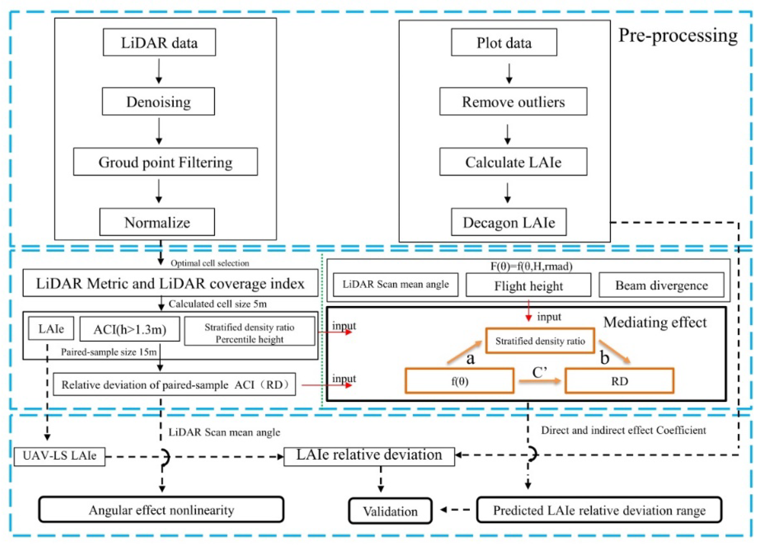
In this paper, we consider the physical parameters of the UAV-LS system and the vertical structure variables of the forest to analyze the effect of UAV-LS angular effects on the estimation of vegetation variables. (1) Using UAV-LS data, a relationship model involving LiDAR system parameters, forest vertical structure parameters, and angular effects was built, and mediating effects were used to analyze the paths and magnitudes of the angular effects on vegetation variables. (2) The contribution of angular effects to estimates of the relative bias of vegetation variables was explored (the flow chart is shown in Figure 2).

2. Materials and Methods

2.1. Study Area

This study was performed in the Duraer National Forest in Arxan, northeastern China (47°15′–47°35′ N, 119°28′–120°01′ E). This site is an important ecological protection area in China located at the western foot of Greater Khingan and is bordered by the Mongolian Dongfang Province to the west and Hulunbeier Steppe to the north. The forest covers a total area of 49,812 hectares, and elevations range from 792 to 1475 m. The forest is dominated by Betula platyphylla and Larix gmelinii. There are many downed and standing deadwood areas on the peaks above 1000 m. The structure of the study area is complex due to natural disturbances and noninterventionist management policies (Figure 3).

2.2. Plot-Level Data Estimates

Decagon’s AccuPAR LP-80 (Decagon Devices Inc., Pullman, WA, USA) instrument was used due to the complex topography and weather variability in the study area. The acquisition of data required that areas of the high canopy be without senescent vegetation and display good uniformity and low spatial heterogeneity as sample plots [29]; therefore, pure forest stands at the edge of the forest were selected. The data were collected in July 2021 at the locations marked with red dots in Figure 3, totaling 80 sample plots (only 62 sets of anomaly free data were used due to the sensor being affected by direct sunlight). The solar zenith angle range was 21°–60°; the measured positions were recorded using a differential GPS device during the recording process. In this study, we used the photosynthetic active radiation (PAR) measured in unshaded clearings or larger forest windows instead of the incident photosynthetic active radiation above (PARa) from the upper part of the tree canopy. Canopy PAR measurements were obtained only at the beginning and end of each data collection period, and we found it best to first calculate the average PARa for photosynthetic active radiation below (PARb) in the lower portion of each canopy. The parameters were collected at four uniformly recorded points within each sample plot and were measured three times consecutively to obtain the in-sample variables (e.g., PARa, PARb, fb, and θ) that were needed for Decagon’s AccuPAR LP-80 algorithm to calculate the LAI by constantly moving among multiple locations within the sample plot to decrease the canopy aggregation [30] (the data collection information is shown in

Table 1. Plot-level data.

Plot Count	Vegetation Type	Dominant Tree Species	LAIe Range	Min	Max	Mean
18	Coniferous	Larix gmelinii (Rupr.) Kuzen	2.57–3.43	2.57	3.43	3.06
8	Mixed	Betula platyphylla Suk., Populus davidiana Dode	2.28–2.7	2.28	2.7	2.57
36	Broadleaf	Betula platyphylla Suk.	1.55–3.05	1.55	3.05	2.40

). AccuPAR is sensitive to light conditions, and indirect light increases the sensitivity of acquisition parameters and measurement errors; thus, AccuPAR should be used preferentially under diffuse light conditions [29,31] (refer to Supplementary Section S1 for detail information).

The 5 parameters that were obtained using Decagon’s AccuPAR LP-80 at the plot level were then applied to calculate the LAI_e values based on a modified version of the canopy light transmission and scattering model that was developed in Ref. [32]:

$$L=\frac{[(1-(1/2K)){\mathrm{f}}_{\mathrm{b}}-1]\ln \mathsf{\tau }}{0.9(1-0.47{\mathrm{f}}_{\mathrm{b}})},$$

(1)

$$K=\frac{{({\chi }^2+{\tan }^2\theta )}^{1/2}}{\chi +1.744(\chi +{1.182}^{-0.733})},$$

(2)

where f_b is the fraction of direct (non-diffuse) radiation; τ is the canopy transmittance (transmitted PAR/incident PAR); K is the extinction coefficient; χ is the leaf angle distribution, which is defined as the ratio of the horizontal to vertical axes of the ellipsoidal leaf distribution [30]; and θ is the solar zenith angle. Because the obtained parameters are inclusive of the non-photosynthetic component and aggregation effects, the obtained LAI is calculated as the LAI_e [33,34,35].

2.3. UAV-LS Data and Preprocessing

All of the UAV-LS data in the study were obtained from a Haida six-rotor UAV Long-120 equipped with a Haida ARS-1000 L long-range LiDAR measurement system (Haida Zhong, Wuhan, China). The core parameters of the LiDAR sensor in this system are listed in Supplementary Section S3. LiDAR data were obtained from 12 July to 17 July 2021, and covered seven transects in the study area, with a total coverage area of 21.8 km². The platform flew at altitudes between 200 and 400 m, with flight speeds of 6–10 m/s and overlaps of 60% in the side direction and 70% in the heading direction. The LiDAR sensor beam divergence fraction was 0.5 rmad, so the acquired data footprint diameter varied from 0.1 to 0.2 m; additionally, the average point density of five data strips was greater than 60 points/m², and that for two data strips were greater than 30 points/m², thus meeting the point cloud density requirements of this study [22,36]. Four of the LiDAR strips included crossover areas, and the flight parameters remained consistent. It is worth noting that, for the same forest plot, based on the scanning parameters and subsurface (forest type), resampling to decrease the point cloud density introduced more uncertainties in some cases. Therefore, the raw data without resampling were used in this study.

We applied a series of processing steps, such as denoising, classifying ground points, filtering classification, and normalization based on ground points, to the data with LiDAR360 software (Green Valley, Beijing, China); then, we obtained gap-free canopy height model (CHM) data [37]. To facilitate data mapping and normalized representation, the data were gridded, and the tested grid sizes were 3 m × 3 m, 5 m × 5 m, 10 m × 10 m, 15 m × 15 m, and 20 m × 20 m. Uncorrected LAI_e values were calculated for each grid cell to test the accuracies of the point cloud representations within the grid, and subsequent experiments were conducted on the grid with the highest accuracy.

2.4. LiDAR-Derived Variables and LAI Model

2.4.1. LiDAR Cover Index and Point Cloud Height Variables

The interactions between the forest canopy and laser pulses can be considered to be similar to the interactions between the forest canopy and direct beam solar radiation, and LiDAR calculations of the forest vertical structure parameter variables are indirectly considered to be valid proxies for those of real forest structures [38]. In this context, the canopy cover (CC) and canopy gap fraction (GF) are usually approximated by various laser indices. In this study, we instead calculated three LiDAR indices, namely, the first echo cover index (FCI), last echo cover index (LCI), and all echo cover index (ACI), to approximate the vertical gap fraction (see

Table 2. LiDAR cover indices.

Equation	Reference
$FCI=\frac{{\displaystyle \sum N_{Single\_canopy}+{\displaystyle \sum N_{First\_canopy}}}}{{\displaystyle \sum N_{Single\_all}+{\displaystyle \sum N_{First\_all}}}}$	[14]
$LCI=\frac{{\displaystyle \sum N_{Single\_canopy}+{\displaystyle \sum N_{L\mathrm{a}st\_canopy}}}}{{\displaystyle \sum N_{Single\_all}+{\displaystyle \sum N_{Last\_all}}}}$	[20]
$ACI=\frac{{\displaystyle \sum N_{\mathrm{groud}}\left(\mathrm{H}>\mathrm{h}\right)}}{{\displaystyle \sum N_{\mathrm{all}}}}$	[11]

). Additionally, because of anomalies in the data echo information at the center of the transect, no Sorlberg cover index (SCI) values were calculated.

In the above equations, h = 1.3 m (as specified by the height at which Decagon’s AccuPAR LP-80 measurement data were obtained). In addition, we calculated the percentiles of the UAV-LS height distribution (e.g., P10, P20, P50, P90, and P99) and the stratified density (e.g., D1, D2, D3, D3, D4, D5, D6, D7, D8, D9, and D10) vegetation variables. The point clouds in the statistical cells were equally divided into ten layers in the vertical direction above the ground, and the point clouds in each layer accounted for a proportion of all point clouds. The accuracy of the ACI calculations was mainly influenced by the scanning angles and vertical forest structures. The ACI is different from the FCI, and the ACI expresses the variations in forest vegetation points above a certain height and encompasses three-dimensional information related to the forest structure.

2.4.2. UAV-LS LAI Estimation Model

LAI calculation methods based on the Beer–Lambert law have been widely used [14,15,39]. Such an approach was initially used to describe light attenuation in a homogeneous medium and was further extended to light interception in a homogeneous canopy [40]. The LAI versus gap fraction at a given zenith angle can be expressed as follows [31]:

$$P(\theta )=e^{-G(\theta )\mathrm{L}\mathrm{A}\mathrm{I}/\mathrm{c}\mathrm{o}\mathrm{s}(\theta )},$$

(3)

From the above equation, the formula for the effective leaf area index can be derived [39]:

$$L_{\mathrm{e}}=-\frac{\cos ({\stackrel{-}{\theta }}_{L\mathrm{i}DAR})}{K}\ln (P(\theta )),$$

(4)

where L_e is the effective leaf area index, θ_LiDAR is the cosine function of the mean LiDAR scanning angle, K is the extinction coefficient, and P(θ) is the clearance rate for a specific zenith angle.

The vegetation variables that are extracted from LiDAR data are affected by the vegetation cover and LiDAR angular effects, which result in the underlying information being underrepresented in the discrete point cloud data and greater amounts of missing data as the scanning angle increases. However, some of the indices are relatively stable up to 20 degrees [21,41], so the LiDAR coverage index was used to calculate LAI_e instead of the gap rate (Equation (4)). According to a relevant study by Hu et al. [42], it is known that the ACI effectively balances the contributions between the first and last echoes among the various laser coverage indices. The ACI was calculated using the threshold method with a value of 1.3 m (i.e., the height at which AccuPAR measures the canopy parameters) above the vegetation point and below the ground point applied for LAI_e calculations (see Equation (5)).

$$L_{\mathrm{e}}=-\frac{\cos {\stackrel{-}{\theta }}_{lidar}}{K}\ln (1-\mathrm{ACI}),$$

(5)

2.5. Concretization of Angular Effects

2.5.1. Relationship Model of Angular Effects

The discrete point cloud data that are collected by LiDAR systems under ideal conditions usually reflect the real structures of surface relief and forests (both the vertical and horizontal structures), but the LiDAR system used, route design, and forest type all affect the actual point cloud distribution, which results in angular effects. Among them, the scanning angle generated by the LiDAR system and the route design highly influence the generation of angular effects. The angular effects in this study represent the differences in ACI due to the differences in angle.

The acquired UAV-LS data are based on acquisitions of small areas, and the increase in scanning angle and increase in amplitude during the progression from the center of the route to the edge of the route in a single transect (i.e., without transect overlap) lead to increases in angular effects. The changes in scanning angle during the acquisition process consist of the following: (1) Ground points and the lower parts of the trees are often blocked by the trunks and canopies of adjacent trees, especially in areas with large undulations; this is reflected in the data by the absence of point clouds on the other sides of trees and in shadowed areas on the ground (Figure 1a,b and Figure 4). (2) It is very difficult to completely capture the vertical information of the forest at nadir; the amount of vertical tree information that can be obtained increases as the scanning angle increases, and more point clouds are obtained from the side. (3) We did not consider intensity variations or the reflectance information associated the discrete point cloud data and analyzed only the angular effects based on the structures reflected by the discrete point cloud data.

The covariations in the vegetation variable (VV) that are caused by changes in the scanning angle and vegetation structure during data generation by the UAV-LS system cause the number of discrete point clouds and the proportions of point cloud types to vary; ultimately, we infer that the magnitudes (Mag) of the angular effects are a function of the scanning angle function and VV.

$$\mathrm{Mag} =F\left(f\left(\theta \right),VV\right),$$

(6)

We used the mean scanning angle of the point cloud for each paired sample as an approximate proxy for the scanning angle of each statistical cell [18]. For the VV, several percentile height variables and stratified density variables were obtained from the LiDAR data to represent the forest structure variables. The percentile heights and stratified density variables are reasonable indicators because of these variables. The height or stratum at which a change occurred that resulted in a difference in ACIs based on different scanning angles and forest structures can thus be determined. The magnitudes of the angular effects based on the selected scanning angle function and forest attributes (e.g., aggregation distribution and tree species) are ultimately expressed in terms of the number of point clouds or point cloud-based LiDAR variables. To further investigate the effect of the scanning angle function on the ACI magnitude, the quantified Mag is expressed using the relative deviation (RD), which is the absolute value of the quotient of the difference between the ACIs obtained from two different scanning angles within the same statistical cell and the ACIs obtained at smaller scanning angles [43]. Here we consider that Mag and RD are numerically equivalent, and the latter content involves the angular effect with RD instead. In Equation (7), y indicates the ACI acquired in the vertical direction, and Y indicates the ACI acquired in the horizontal direction. The larger the RD value, the greater the quantified magnitude of the ACI in the paired statistical analysis, and the more the ACI is affected by the angular effects in the cell.

$$\mathrm{RD} =|y-Y/y|,$$

(7)

2.5.2. Statistical Method for Analyzing the Magnitudes of the Angular Effects

The angular effects not only directly influence the RD but also indirectly affect the types and numbers of discrete point clouds at different altitudes. Additionally, considering the sensor properties, route height coupling is important, and we define this combined effect based on the LiDAR effect area (LEA) (Figure 1a,b) that is captured by the LiDAR system; i.e., the LEA represents the area in which effective information can be captured by a specific LiDAR system for a certain forest structure. To calculate the LEA, we express the relationship between the scanning angle and the number of point clouds as a function of the ratio of the projected area obtained for trees in the statistical cell at a smaller scanning angle and at a large off-nadir angle. Finally, we conclude that the product of the route height and laser beam divergence fraction divided by the square of the cosine of the scanning angle can effectively express the relationships between the system parameters and point cloud density.

Mediating analysis is applied to investigate how f(θ) affects the magnitude of the angular effect. As descried in the conceptual model, RD is a function of VV and f(θ). VV is also influenced by f(θ). Therefore, the causal chain of f(θ) affecting the angular effect through the third variable VV may hold. The use of an independent variable to obtain the predictor variable through a third variable is a mediating effect, and the third variable is called the mediating variable [44]. In this research, we use the magnitude of RD as the dependent variable, f(θ) as the independent variable, and VV as the mediating variable. According to the mediation analysis method [45], the overall relationship we observed between landscape factors and angular effect sizes (labeled as total effects in Figure 5a) consisted of two pathways (Figure 5b): (1) the indirect effect, in which f(θ) leads to the RD through VV; and (2) the direct effect, in which f(θ) leads to the RD directly, regardless of the mediator.

By estimating the indirect and direct effects and testing their significance, we revealed the path and intensity of the influence of f(θ) on the angular effect. The classical statistical mediation testing method proposed by Baron and Kenny [44] has been widely used and proven to be a practical approach for assessing mediating effects. In this research, we adopted this approach and established the following three regression equations to examine mediation (Equations (8)–(10)):

$$\mathrm{RD}=\mathrm{c}f\left(\theta \right)+\epsilon ,$$

(8)

$$VV=af\left(\theta \right)+\epsilon ,$$

(9)

$$\mathrm{RD} =c^{\prime }f\left(\theta \right)+b VV+\epsilon ,$$

(10)

$$f\left(\theta \right)=H\times \mathrm{rmad}/\cos \left(\theta \right),$$

(11)

In Figure 5, VV is replaced by the percentile height or stratified density variable for a paired sample; RD is the relative deviation of the paired ACIs in the relational model with angular variations; f(θ) represents the functional relationship among the scanning angle, flight height, and the laser beam divergence fraction; ε is the error term; and a, b, c, and c′ are the coefficients of each regression equation, where c = a × b + c′. Notably, a, b, and c′ are defined in Figure 5. To verify the presence of mediating effects, we use the test procedure that was proposed by Wen and Ye [46], where the direct effect coefficient, i, and indirect effect coefficient, j, obtained from the mediating effects, are added as model weights to the angular effects correction model, where i + j = 1.

$$\mathrm{RD} =if\left(\theta \right)\times jVV+\epsilon ,$$

(12)

2.5.3. Experimental Design for the Quantification of Angular Effects

The transect intersection areas were used for the UAV-LS data analysis and were calculated with the ArcGIS Pro2.8 (ESRI, San Diego, CA, USA) Fishnet tool as a statistical window at a cell size of 15 m. This window was used to obtain a 3 × 3 grid with a cross-region cell size of 5 m for the preprocessed data based on the ACI by scanning the mean angles. The selected paired samples were located in forest areas and fully covered by point clouds, and those sample points with abnormal ACI differences between non-forest areas and point clouds due to incomplete coverage were excluded (samples with ACI values less than 0.5 and ACI differences greater than 0.3 were excluded due to incomplete coverage of the sample pairs, as specified in Supplementary Section S2). To amplify the ACI differences due to angular effects and ensure the accuracy of the ACI calculations, the samples with the largest angular differences between two scans within the same paired sample and with sample point cloud densities greater than 10 pts/m² [20,36] were used, and the final number of modeled samples was 425 pairs (Figure 6). A paired-sample Kruskal–Wallis test between vertical transect and horizontal transect directions’ extracted ACI values was conducted to determine if a statistically significant difference existed. The H0 hypothesis was “there is no difference between the two ACI values from two scanning angles”. The H1 hypothesis was “there is a difference between the two ACI values from two scanning angles”. The level of significance was p < 0.05.

3. Results

3.1. Calculation Results for Plot-Level and UAV-LS Data

The parameters obtained from the instrument were calculated to obtain the LAIs (Figure 7a), and LiDAR mean scanning angles (Figure 7b) for the sample sites.

Figure 7a shows the LAI_e distribution obtained from the actual measurements. There were 62 samples after outlier removal, and they contained 36 broadleaf forest plots, 18 coniferous forest plots, and 8 broadleaf mixed forest plots, with a mean value of 2.70. The distribution of the mean scanning angle of the LiDAR data for the 62 sample plots is shown in Figure 7b, and the mean scanning angles are nearly all greater than 10°, with an overall mean scanning angle of 15.83°.

3.1.1. Statistical LiDAR Cell Size Comparison

The distributions of ground and vegetation points (Figure 8) at different sampling resolutions were obtained according to the classification results in Section 2.3 (sampled at the exact center with expanded sides).

The statistical variables, standard deviations, correlation coefficients, and RMSDs were calculated between the LAIe values that were extracted by UAV-LS and the measured LAIe values, and the best grid was selected from the 3, 5, 10, 15, and 20 m resolutions based on the absolute distance to the reference point (Ref) at different resolutions. Based on this analysis, a resolution of 15 m yielded the best result (Figure 9).

3.1.2. UAV-LS Metrics

The histogram of the ACI frequency distribution obtained from vertical transects and horizontal transects for the paired samples introduced in Section 2.5.3 is shown in Figure 10.

Subsequently, the paired-sample Kruskal–Wallis test result between the vertical and horizontal transect ACI differences was significant (chi-squared = 7.8476 > 6.635, p-value < 0.01). This finding indicated that there was a significant difference between the ACI values extracted from the vertical and horizontal transects within the same paired sample.

Table 3. Multiple tests of density metrics at different scanning angles.

Adj.p-Value	D1	D2	D3	D4	D5	D6	D7	D8	D9	D10
0_6°–6_21°	1.000	1.000	0.38	0.061	1.000	1.000	0.167	1.000	1.000	0.91
6_21°–21°_max	0.387	0.000 **	0.000 **	0.000 **	0.000 **	0.45	0.0021 **	0.0004 **	1.000	1.000
0_6°–21°_max	0.019 *	0.29	0.98	0.049 *	0.041 *	1.000	1.000	0.582	1.000	1.000

p < 0.05 *; p < 0.01 **; and the values in the table are the adjusted p-values from pairwise Wilcoxon rank sum tests (using the Bonferroni method).

demonstrates the differences between the same parameters at different scanning angles. The table clearly shows that the stratified density parameters differed most significantly between 6_21° and 21°_max (p-value < 0.01), suggesting that the vegetation information obtained in the ranges of D2–D5 and D7–D8 was affected by the selected scanning angles.

The differences among P10, P20, P50, and P90 obtained in

Table 4. Results of multiple tests of common LiDAR metrics at different scanning angles.

Adj.p-Value	Height LiDAR Metrics						Canopy Cover
	P10	P20	P50	P90	P99	Elev_min
0_6°–6_21°	0.002 **	0.000 **	0.000 **	0.000 **	0.701	1.0	1.0
6_21°–21°_max	0.000 **	0.000 **	0.000 **	0.000 **	0.653	0.76	0.000 **
0_6°–21°_max	0.125	0.357	0.13	0.12	0.17	0.85	0.001 **

p < 0.01 **; and the values in the table are the adjusted p-values from pairwise Wilcoxon rank sum tests (using the Bonferroni method).

are significant (p-value < 0.01) for the 0_6°–6_21° and 6_21°–21°_max groups but not for the 0_6°–21°_max group, indicating that P10, P20, P50, and P90 yield more accurate percentile heights at 6_21°. The canopy cover varies more as the scanning angle increases. P99 and Elev_min, in contrast, are not sensitive to the scanning angle.

Table 5. KW test of coniferous and broadleaf forests for stratified density variables from LiDAR data at different scanning angles.

	D1	D2	D3	D4	D5	D6	D7	D8	D9	D10
0_6°	0.96	1.927	1.707	0.427	6.827 **	5.23 *	0.027	8.64 **	0.06	0.06
6_21°	22.343 **	21.276 **	11.753 **	8.952 **	2.207	0.78	41.219 **	34.209 ***	43.793 **	48.883 **
21°_max	28.914 **	26.944 **	17.682 **	12.858 **	0.137	3.3231	8.989 **	22.728 ***	18.218 **	42.315 **

p < 0.05 *; p < 0.01 **; the values in the table are chi-squared values (DoF = 1), and the critical chi-squared values at 0.05 and 0.01 significance levels are 3.841 and 6.635, respectively.

and

Table 6. KW test of coniferous and broadleaf forests for stratified density variables from LiDAR data at different scanning angles.

	Height Metrics						Canopy Cover
	P10	P20	P50	P90	P99	Elev_min
0_6°	2.94	1.5	0.027	0.54	0.54	2.415	1.927
6_21°	0.522	7.352 **	45.039 **	51.234 **	3.546	1.581	3.855
21°_max	16.124 **	14.016 **	28.474 **	49.948 **	6.532 *	9.923 **	21.247 **

p < 0.05 *; p < 0.01 **; the values in the table are chi-squared values (DoF = 1), and the critical chi-squared values at 0.05 and 0.01 significance levels are 3.841 and 6.635, respectively.

show the results of the KW experiments comparing LiDAR measurements between coniferous and broadleaf forests. The majority of the variations in the metrics are insignificant in the 0–6° range. The discrepancies between D1–D7 and at low-percentile heights become significant (p-value < 0.01) when the angle reaches 6_21° or even 21°_max. This result suggests that, as the scanning angle increases, the UAV-LS can collect data related to low-level vegetation changes (Figure 11). Contrasting the broad-leaved forest with the coniferous forest, the latter has more vegetation points in the extended lower canopy. In contrast, compared to the coniferous forest, the broad-leaved forest has a more varied understory of plants. Thus, in the subcanopies of both forest types, both factors have a considerable impact on the LiDAR measurements.

3.2. Trends and Magnitudes of the Angular Effects

Figure 12a illustrates the outcomes of our RD mutation analysis at the scanned angles using the slope mutation method in conjunction with local extremes (chi-squared = 17.391 > 9.21; p-value < 0.001). Figure 12b shows that the absolute value of the increase in the angular effect increases by approximately 0.05 between 0 and 6 degrees, is steady between 6 and 21 degrees, and increases dramatically above 21 degrees.

The regression equations in Equations (8)–(10) provide the coefficients among f(θ), VV, and RD and the corresponding significance levels, and the test results indicated that no significant relationship existed between the percentile height variable and f(θ) or RD. The statistical correlations between the canopy characteristics and the stratified density factors and the canopy characteristics and the laser penetration height are shown in

Table 7. Results of the three regressions with Equations (8)–(10) from the mediation analysis of angular effects; the coefficients of the clump fixed-effect dummy variables are not presented.

	D1	D2	D3	D4	D5	D6	D7	D8	D9	D10
a	−0.271	−0.344	0.974 **	1.045 ***	1.187 ***	−0.586 **	0.207	1.200 ***	1.817 ***	−0.438 *
b	0.111	0.750	0.669 ***	0.583 ***	0.344 ***	−0.307 **	−0.101	0.071	0.138 **	−0.100
ab/c	-	-	0.100 ***	0.089 ***	0.041 ***	0.024 ***	-	-	0.052 ***	-
	f(θ)	SumD3-5	SumD3-4	SumD3-6
a	-	3.205 ***	2.019 ***	2.619 ***
b	-	0.223 ***	0.345 ***	0.179 ***
ab/c	-	0.101 ***	0.105 ***	0.066 ***
RD	5.230 ***

p < 0.05 *; p < 0.01 **; p < 0.001 ***; a represents the regression coefficient between the stratified density variable and f(θ); b represents the regression coefficient between the stratified density variable and RD; and ab/c is the indirect effect coefficient (the larger the coefficient, the larger the indirect effect).

and

Table 8. Results of the three regressions with Equations (8)–(10) from the mediation analysis of angular effects; the coefficients of the clump fixed-effect dummy variables are not presented.

	D1	D2	D3	D4	D5	D6	D7	D8	D9	D10
a	5.117 ***	5.232 ***	−0.567	−0.943	−1.623 **	4.507 **	0.281	−9.126 ***	−15.674 ***	2.555 ***
b	0.0163	−0.015	0.679 ***	0.598 ***	0.371 ***	−0.411 **	0.098	−0.156 *	0.0246 ***	−0.139
ab/c	-	-			−0.122 ***	−0.373 **	-	−0.288 *	−0.78 ***	-
	f(θ)	SumD5-9	SumD7-9	SumD8-9
a	-	−22.196 ***	−25.081 ***	−24.80 ***
b	-	0.08 **	0.087 **	0.129 ***
ab/c	-	−0.356 **	−0.44 **	−0.645 ***
RD	4.954 **

p < 0.05 *; p < 0.01 **; p < 0.001 ***; a represents the regression coefficient between the stratified density variable and f(θ); b represents the regression coefficient between the stratified density variable and RD; and ab/c is the indirect effect coefficient (the larger the coefficient, the larger the indirect effect).

, respectively. When the significant factors were combined, Sum3-4 displayed the most significant indirect effect (ab/c = +0.1051; p-value < 0.001) in the bootstrap test for D3, D4, D5, D6, and D9. The effects of the laser penetration heigh were found to be significant for D5, D6, D8, and D9, with the largest indirect effect observed for D9 (ab/c = −0.78; p-value < 0.001). In general, the computation of ACI is indirectly influenced by the vertical gradient in all cases (Figure 13).

3.3. LAIe Relative Deviation Estimation and Prediction

The relative difference between the Decagon LAIe and the LAIe of the broadleaf forest without ACI alteration was computed (Figure 14). The illustration clearly shows the maximum negative relative deviation, which is 30% at a scanning angle of 23.78°, and the maximum positive relative deviation, which is 8.4% at a scanning angle of 11.97°.

The relationship between UAV-LS LAIe and Decagon LAIe is strong (R2 = 0.77 and RMSD = 0.215 in Figure 15a). Equation (13) is used to predict the relative deviation in LAIe due to angular effects, and the majority of the actual relative deviations in Figure 15b fall within the range of the predicted relative deviations. With increasing scanning angle, the error typically increases.

$$\mathrm{R}\mathrm{D}=\{\begin{array}{c}1.78\times f(\theta )-0.78\times \mathrm{D}9,\mathrm{Underestimation}\\ 0.895\times f(\theta )+0.105\times \mathrm{Sum}3-4,\mathrm{Overestimation}\end{array},$$

(13)

4. Discussion

In this study, UAV-LS angular effects were analyzed using a conceptual model. The information that the pulse is able to capture changes as the scanning angle changes. To investigate the uncertainty associated with the angular effect in the UAV-LS acquisition of vegetation structure parameters, the impact of the UAV-LS beam irradiation distance and vegetation structure are taken into consideration.

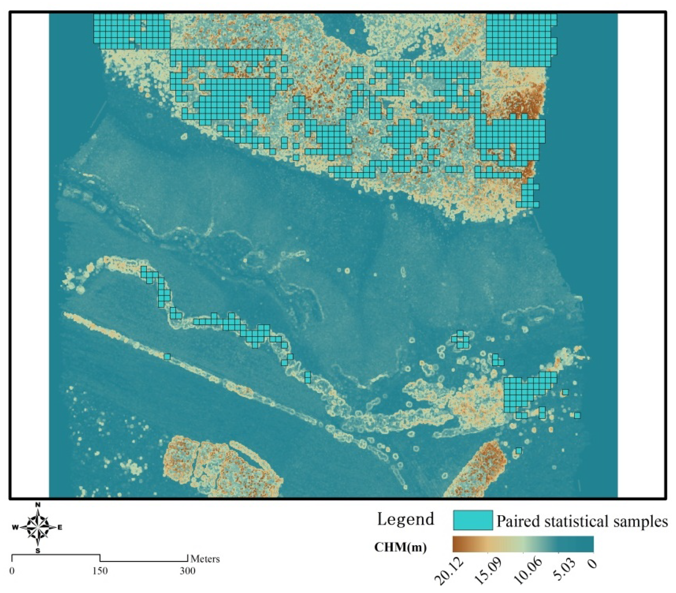
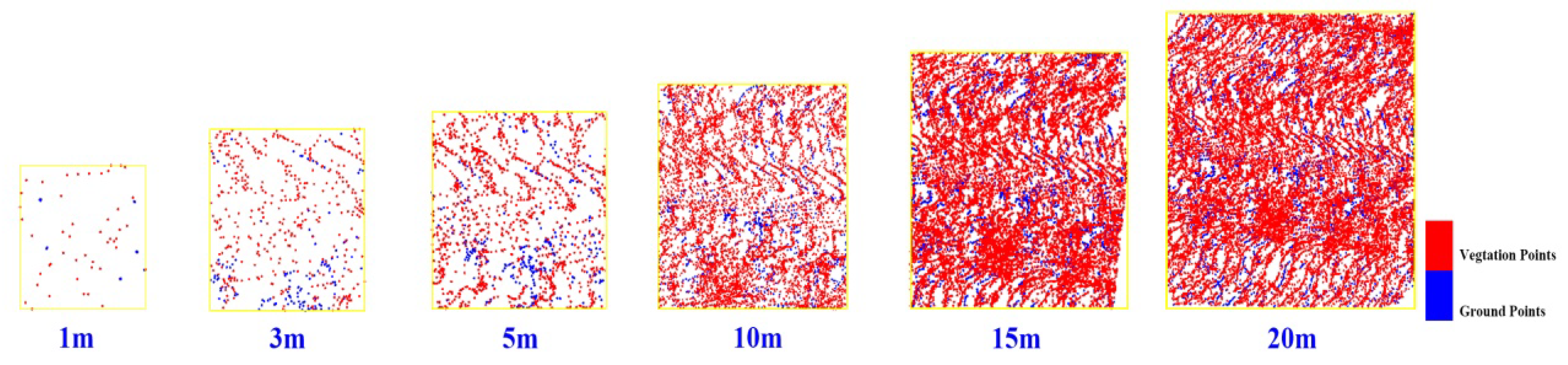
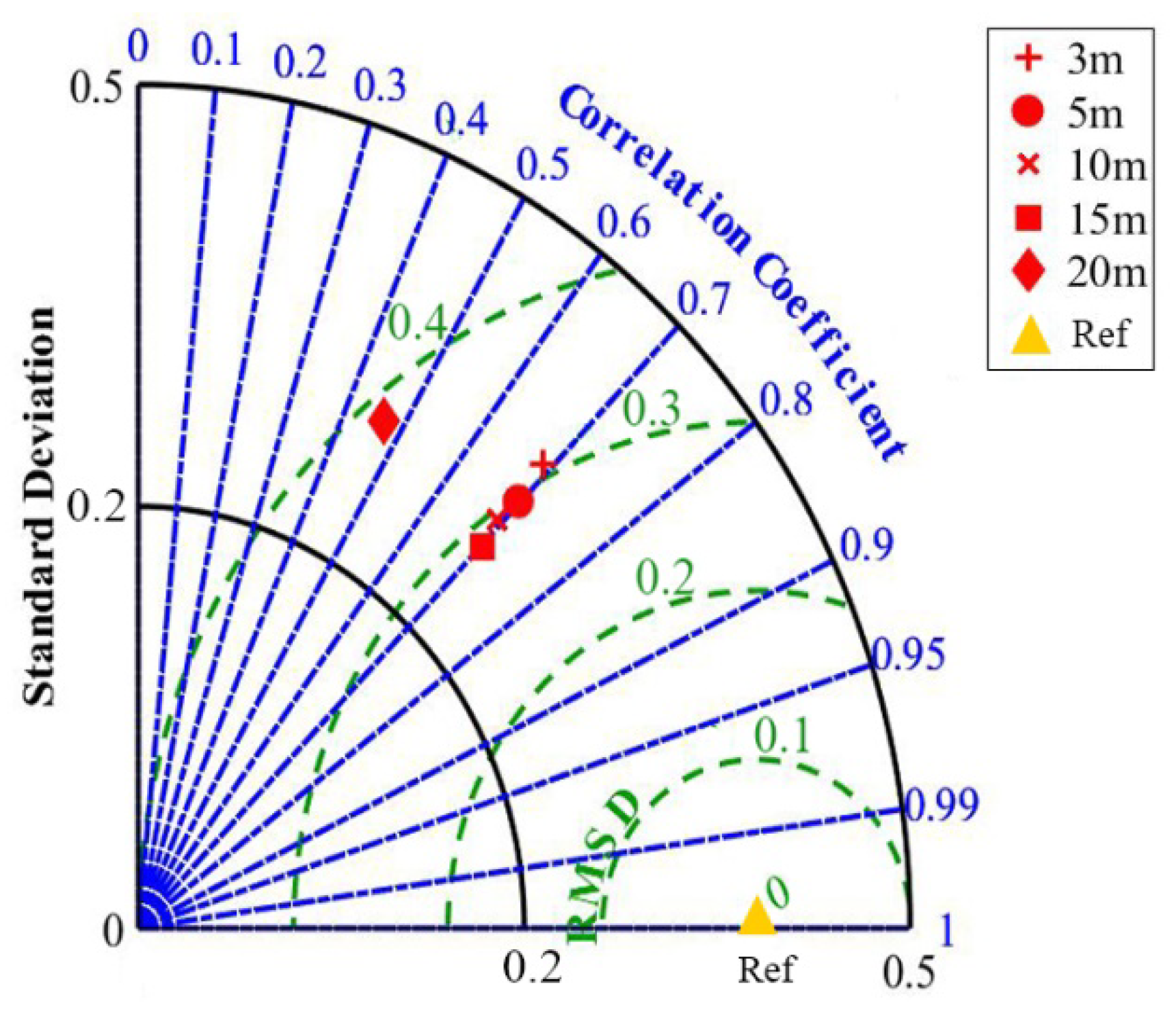
First, the paired sample size is a crucial component when investigating the angular impacts of UAV-LS. Notably, the change in the distribution of points in a raster associated with the shift from discrete point cloud data at a dynamic scale to data in fixed cells influences the accuracy of vegetation structure parameter estimation (Figure 8) [39]. To demonstrate this finding, we performed sensitivity analyses of 3 m × 3 m, 5 m × 5 m, 10 m × 10 m, 15 m × 15 m, and 20 m × 20 m grid sizes. Based on the measured LAIe and the LAIe retrieved by UAV-LS, the highest accuracy was achieved for a 15 m raster size. Therefore, when utilizing LiDAR to produce 2D metrics, we recommend conducting a sensitivity analysis of the LiDAR data conversion scale to determine the optimal size.

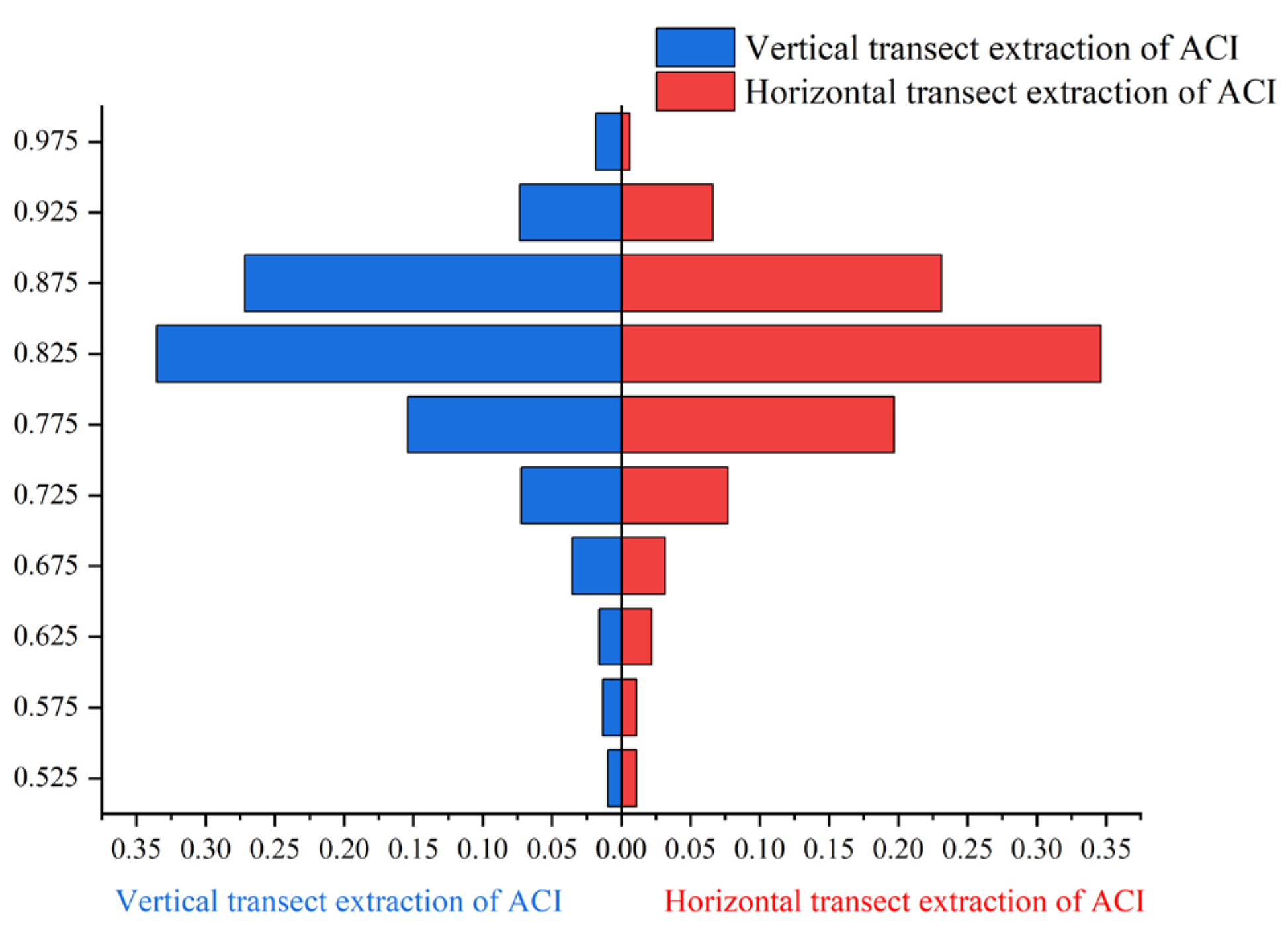
To investigate the uncertainty introduced by the angular effect on the estimation of LAI_e based on the method proposed by Richardson [39], we extracted ACI, stratified density variables, and some common LiDAR metrics. The stratified density variables were used to analyze the influence of angular effects on the density of vegetation points in each layer to determine where angular effects influence the acquisition of vegetation information. We used the 1-ACI approach instead of the gap fraction in this assessment [41]. To measure the impact of angular effects on the amount of vegetation information acquired, height-based LiDAR metrics were used. 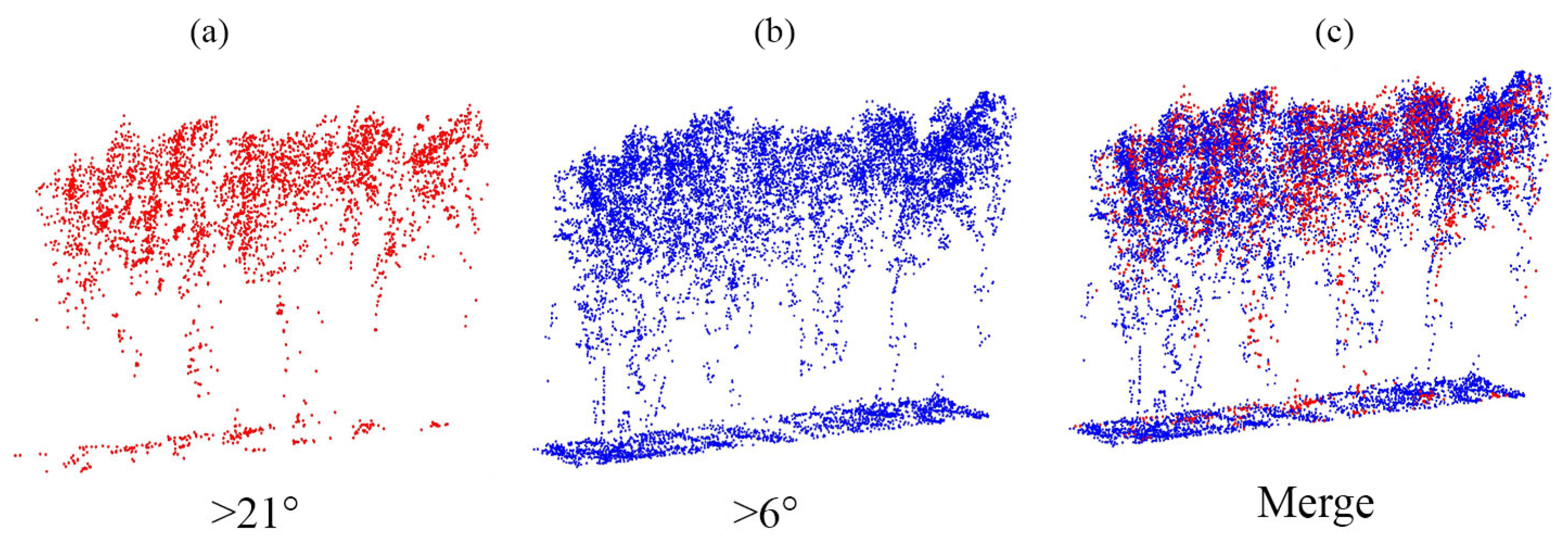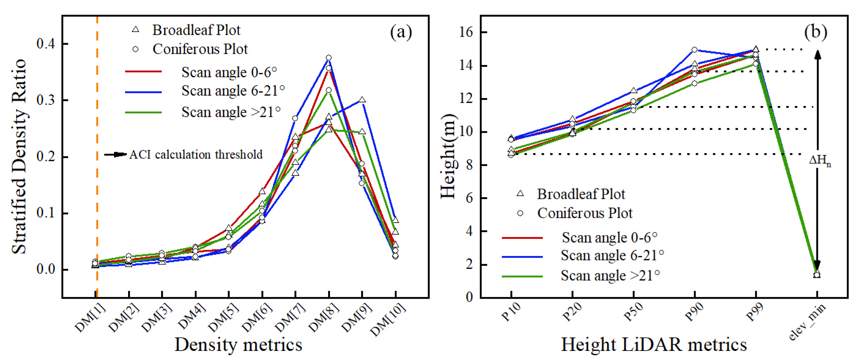Figure 10 shows that the ACI of continuous-cover forest was greater than 0.5 and that the variation associated with the angular effect within the same paired sample did not exceed 0.3 (refer to Supplementary Section S2). The stratification density was significantly different from 6_21°–21°_max for D2, D3, D4, D5, D7, and D8 in the same stand (p-value < 0.001). Due to angular effects, significant differences were observed at different heights in the sub-canopy [47,48] and the height of the forest canopy maximum (Figure 11a). The height-related LiDAR metrics were significantly different (p-value < 0.001) between 0_6°–6_21° and 6_21°–21°_max in several cases, as reported in previous studies [18]. A significant bias in the values obtained when the angle was greater than 21° was estimated based on the canopy cover characteristics [20]. It was concluded from the aforementioned results that larger scanning angles result in more noticeable errors in vegetation structure parameters [22]. Nonetheless, strong effects may be nonexistent at high percentile heights [18]. Coniferous forests are more impacted by scanning angles than are broadleaf forest types, as shown in Table 5 and Table 6 [22] (additionally, in

Table 9. LiDAR metrics for the Kruskal–Wallis test results for broadleaf and coniferous forests at different scanning angles.

CON/BR	P10	P20	P50	P90	P99	Elev_min	Canopy Cover
Chi-squared	59.451 **/31.631 **	60.828 **/40.507 **	68.198 **/49.507 **	71.233 **/54.648 **	5.543/5.4390	2.05/15.653 **	36.099 **/1.629

p < 0.01 **; values in the table are chi-squared values (DoF = 2); the critical chi-squared values at 0.05 and 0.01 significance levels are 5.991 and 9.21, respectively; CON is coniferous forest; and BR is broadleaf forest.

, higher chi-squared values indicate more influence of angular effects). With longer impulse distances through the canopy at incidence angles that diverge from the nadir, coniferous forests typically have canopies that are longer and more densely distributed than broadleaf forests [21].

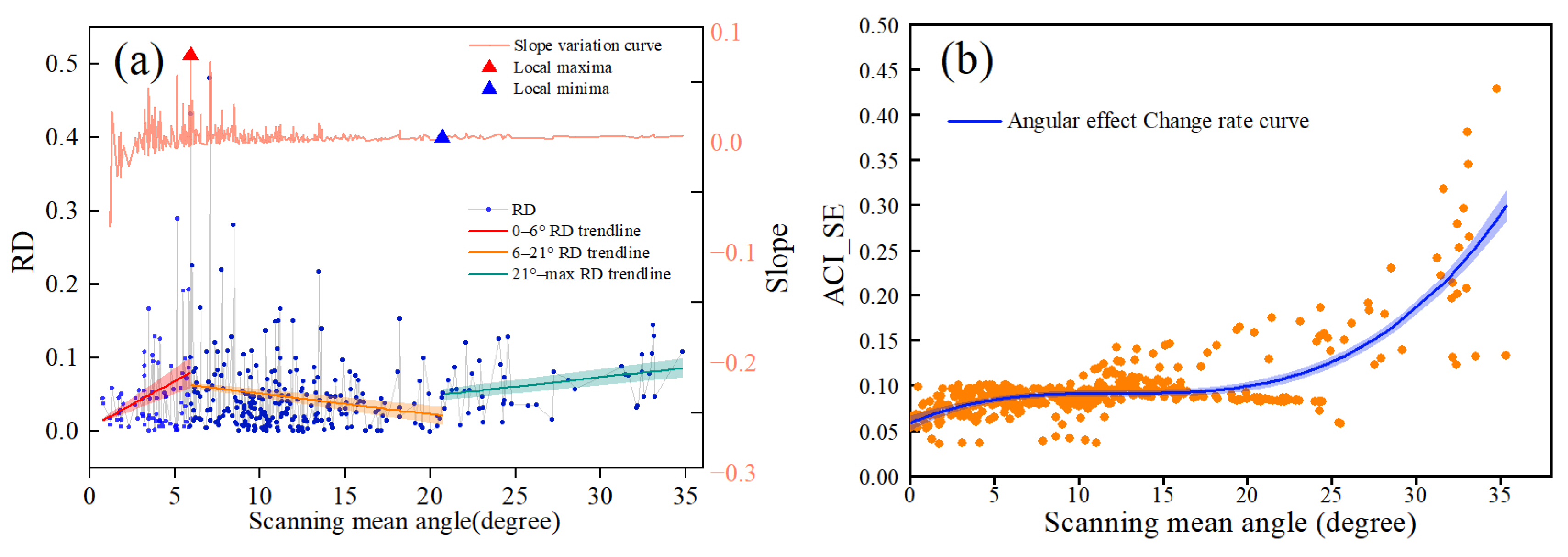
The UAV-LS scanning angle increases from the center of the LiDAR strip to the sides, and the footprint increases with the laser distance to the forest canopy; therefore, the angular effect should increase gradually. The results of the study show (Figure 12) that the angular effect is nonlinear, and the magnitude of the change does not constantly increase [49] (Figure 12b). 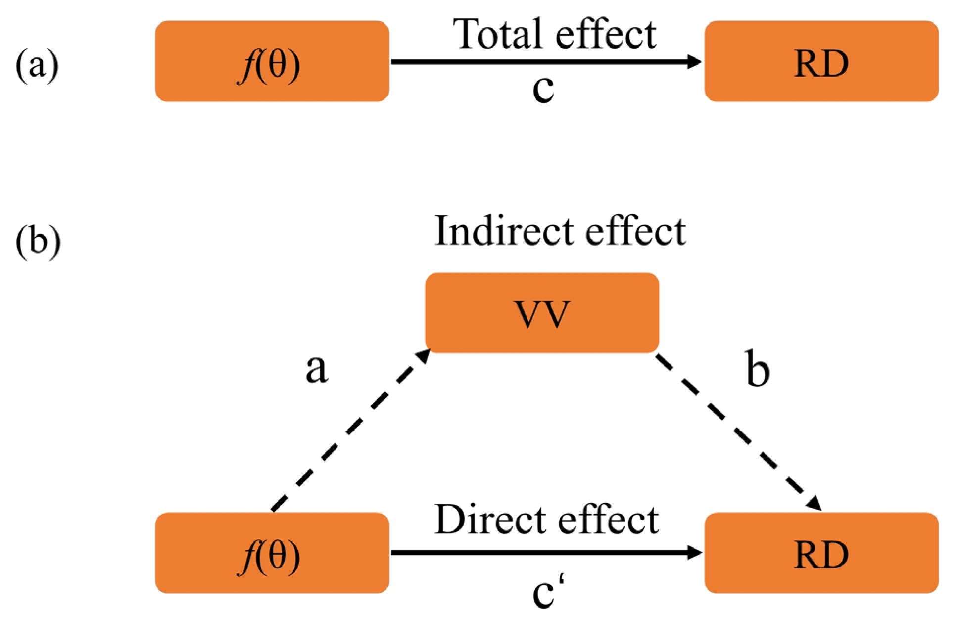This result may be partially because nearby point clouds complement nearby routes with notable angular effects on the nearby strips in the side overlapping sections [25]. Hence, we used mediating effects to analyze the vegetation information obtained by laser beam irradiation to the ground and the top of the canopy to obtain the direct and indirect magnitudes and paths that produce angular effects [49]. The direct relationship between f(θ) and RD that is both positive and highly significant (p-value < 0.001) supports the idea that the primary causes of angular effect are variations in the scanning angle, laser divergence fraction, and flight height [50,51]. When the aerial height is kept constant, as the scanning angle increases, the footprint is stretched in an elongated ellipse, and the angle between the laser beam and the top normal of the canopy increases, which results in vegetation points on the other side of the canopy that are missing or lost (Figure 4). The loss of upper vegetation points caused by the angular effect will undoubtedly result in values that deviate from the actual ACI values. 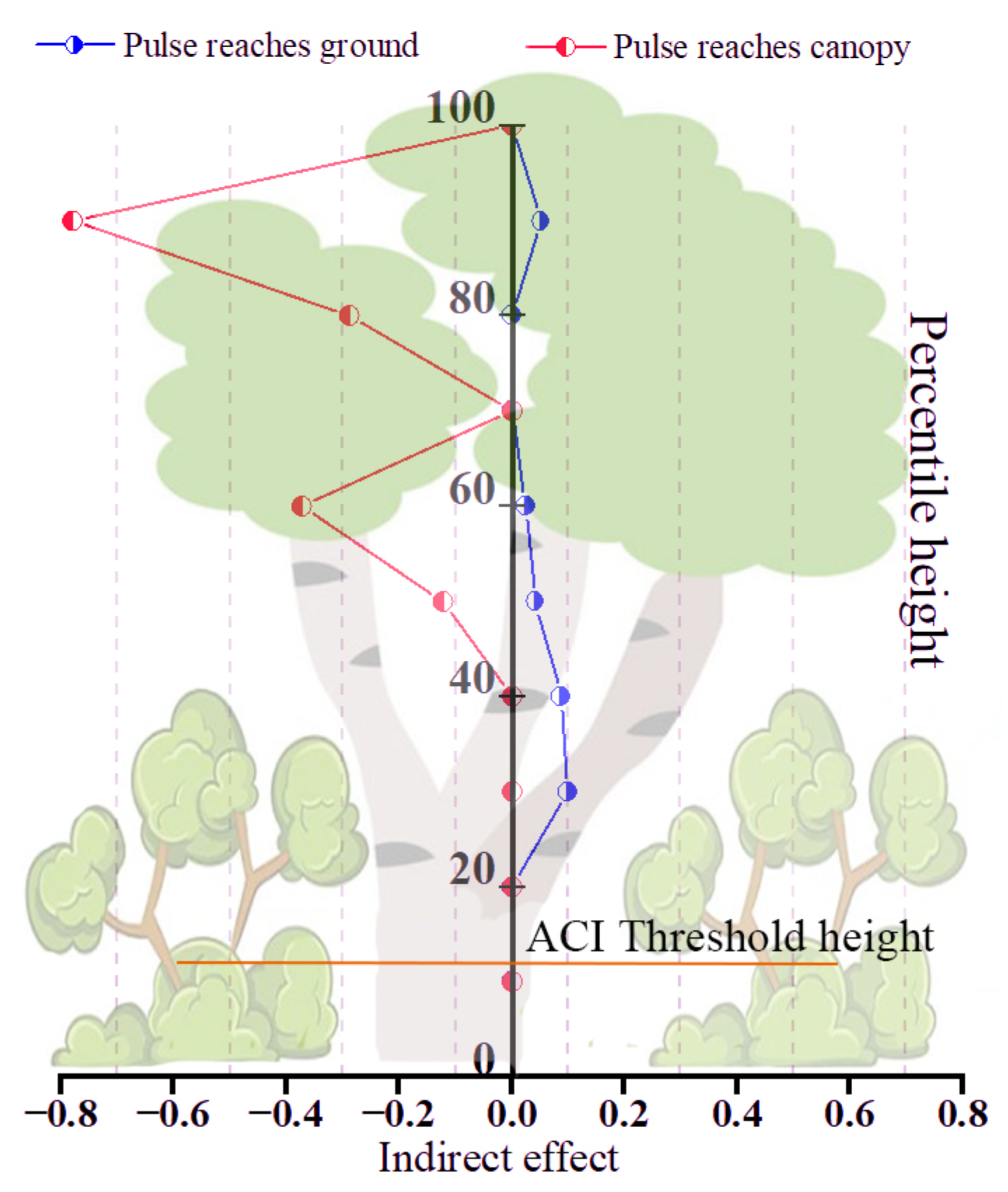Thus, the f(θ) variation contributes to the angular effect. Echoes are generated when a laser beam reaches the ground unobstructed, and the ratio of h > 1.3 m above-ground echoes to all echoes is considered [11]. All the vegetation information obtained from echoes has a positive effect on the ACI. As shown in Table 7, the indirect effect coefficients a and b for D3-D6 are significant (p-value < 0.001), and it is inferred that the vegetation points at the heights of D3, D4, D5, D6, and D9 affect the ACI accuracy. The largest indirect effect is associated with the vegetation points within D3 + D4 (indirect effect coefficient ab/c = +0.105, p-value < 0.001). When the laser beam reaches the upper canopy, a part of the laser beam penetrates unobstructed to the understory and the ground to generate echoes. However, the canopy intercepts a portion of the laser beam to produce negative effects, which creates an obstacle to the ACI calculation. From Table 8, it is concluded that D5, D6, D8, and D9 have a significant negative indirect effect on ACI calculation (p-value < 0.001), and the largest indirect effect was observed for D9 (indirect effect coefficient ab/c = −0.78, p-value < 0.001). We infer that this is due to the combined effect of dense vegetation having a larger backscattering cross-section and a more substantial angular effect masked by the backscattered energy [49]. 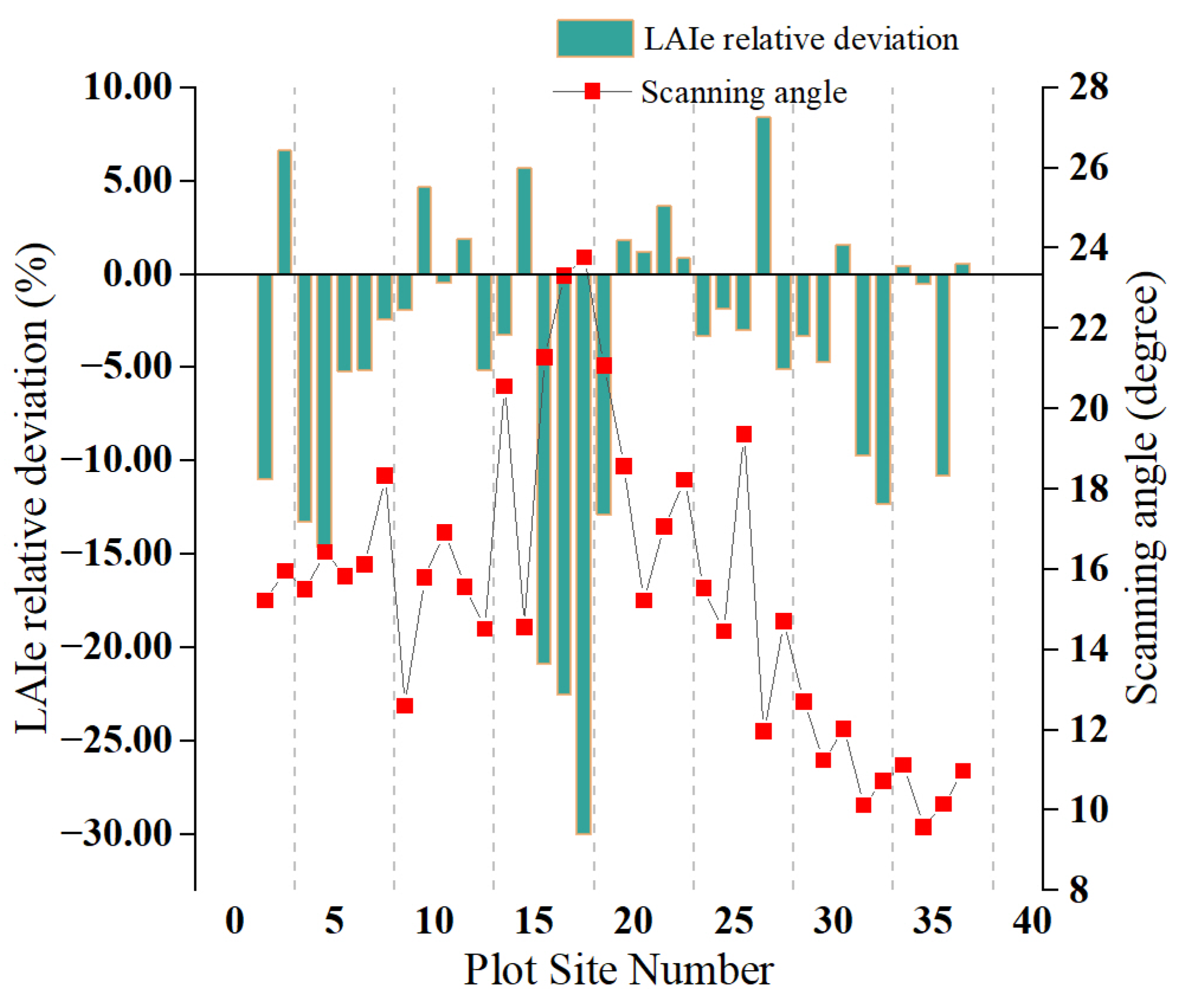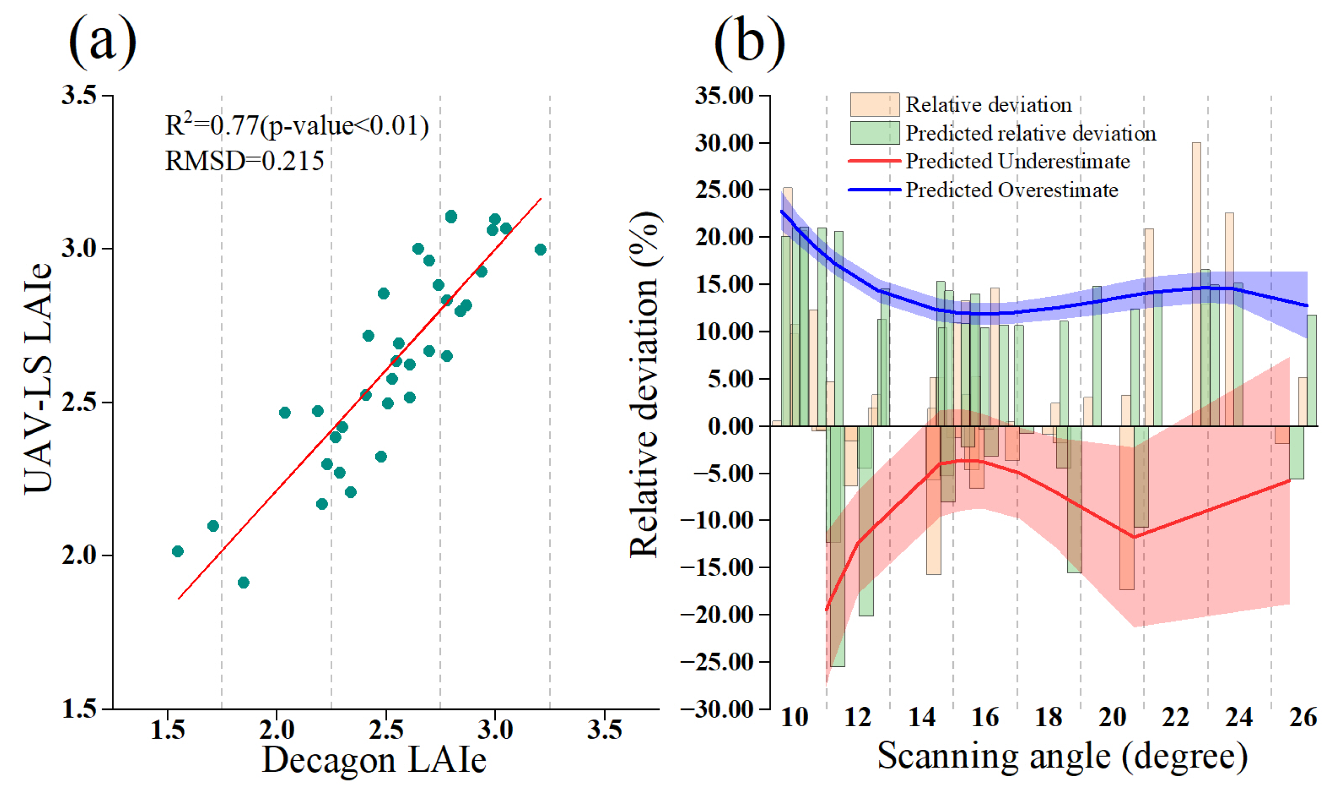By comparing Table 3 and Figure 13, the indirect effects derived from the two results on the vertical gradient coincide. Returning to the experimental sample, due to the data limitation of including only broadleaf forest samples, our LAI_e in UAV-LS broadleaf forest was generally overestimated (Figure 14), and the maximum overestimation was 31% at a scanning angle of 23.78°. Since the relative deviation tends to increase with increasing angle, and the predicted relative deviation from Equation (13) accurately reflects the actual relative deviation between UAV-LS LAI_e and Decagon LAI_e, the predicted relative deviation resulting from the angular effect is rational, as shown in Figure 15. Therefore, we speculate that the actual relative deviation between UAV-LS LAI_e and Decagon LAI_e may range from −25% to 20%.

In the nadir direction, the UAV-LS angular effect is minimized for 2D data, such as canopy cover and gap fraction data, and the scanning angle is not as sensitive to angular effects (Table 4). The circumstances for 3D and 2D data, however, are different. For instance, because of upper-canopy occlusion, it is challenging to obtain high-accuracy 3D data at high-percentile heights and accurate stratified density variables in the nadir direction (Table 4) [22]. Therefore, information from different scanning angles should be obtained to complement the vegetation information and 3D datasets should be established to consider angular effects (Figure 16).

The uncertainty of UAV LiDAR technology was assessed in this investigation. UAV-LS is incapable of capturing comprehensive canopy structure data. TLS data should be incorporated into future investigations to address the problem of missing substructure data in airborne LiDAR measurements. Additionally, the available data sources are lacking, and more data should be considered as they become available. Due to the lack of paired-sample LiDAR data for coniferous forests, it is challenging to assess the inaccuracies induced by angular effects in coniferous forest areas.

The forest structure and the LiDAR system lead to angular effects. An angular effect does not always have a negative impact and may enhance the richness of discrete point cloud data in peripheral vegetated areas within the specified angular range. Consider, for illustration, an airborne LiDAR acquisition operation in which the scanning angle is controlled within the range of 6–21°. To maintain data integrity and the correctness of the information related to the forest structure, multiple air bands that cross each other are employed, or at least two air bands that are perpendicular are used to complement the point cloud data. Despite the additional cost and effort, this approach will reduce the data quality problems due to angular effects, resulting in more accurate landscape-scale LAI_e [25]. Additionally, historical data gathered by LiDAR systems are available for the same forests. Thus, it is possible to compare the interactions of the forest canopy with laser pulses to those of the canopy with a direct solar radiation beam. The change in solar radiation inside the canopy can be thought of as the angular effect. As a result, canopy radiation transmission research can use airborne LiDAR systems in the future. Such systems provide an effective instrument for tracking changes in solar radiation in the canopy structure at various levels [1,52].

5. Conclusions

Angular effects have been shown to often occur during the collection of vegetation metrics data by UAV-LS. Therefore, we investigated the angular effect and its drivers. First, we proposed a relational model of the angular effect, hypothesized about the mechanisms that shape the angular effect, and extracted the vegetation structure indicators that the angular effect may influence. Second, we analyzed the factors and pathways associated with the angular effect using mediating effects, and quantified the direct and indirect effects, particularly the magnitude of the angular effect in broadleaf forests.

Based on the results, the following conclusions were obtained: (1) The use of physical LiDAR parameters (aerial height, laser divergence fraction, and scanning angle) and forest vertical structure variables results in some of the deviations in the LAIe extracted by UAV-LS compared to the Decagon LAIe due to the angular effect of UAV-LS. (2) The indirect angular effect is negative for the upper canopy and positive for the understory part of the continuous and closed vertical gradient of the forest. (3) Multi-angle LiDAR data can be used to establish three-dimensional vegetation indices.

References

1. Olpenda, A.S.; Stereńczak, K.; Będkowski, K. Estimation of sub-canopy solar radiation from LiDAR discrete returns in mixed temporal forest of Białowieża, Poland. Int. J. Appl. Earth Obs. Geoinf. 2019, 79, 116–132. [Google Scholar] [CrossRef]
2. Zhang, X.; Bao, Y.; Wang, D.; Xin, X.; Ding, L.; Xu, D.; Hou, L.; Shen, J. Using UAV LiDAR to Extract Vegetation Parameters of Inner Mongolian Grassland. Remote Sens. 2021, 13, 656. [Google Scholar] [CrossRef]
3. Wang, Y.; Weinacker, H.; Koch, B. A Lidar Point Cloud Based Procedure for Vertical Canopy Structure Analysis And 3D Single Tree Modelling in Forest. Sensors 2008, 8, 3938–3951. [Google Scholar] [CrossRef] [PubMed]
4. Lefsky, M.A.; Cohen, W.B.; Parker, G.G.; Harding, D.J. Lidar Remote Sensing for Ecosystem Studies. BioScience 2002, 52, 19–30. [Google Scholar] [CrossRef]
5. Lin, Y.; Wiegand, K. Towards 3D tree spatial pattern analysis: Setting the cornerstone of LiDAR advancing 3D forest structural and spatial ecology. Int. J. Appl. Earth Obs. Geoinf. 2021, 103, 102506. [Google Scholar] [CrossRef]
6. Guo, Q.; Su, Y.; Hu, T.; Guan, H.; Jin, S.; Zhang, J.; Zhao, X.; Xu, K.; Wei, D.; Kelly, M.; et al. Lidar Boosts 3D Ecological Observations and Modelings: A Review and Perspective. IEEE Geosci. Remote Sens. Mag. 2020, 9, 232–257. [Google Scholar] [CrossRef]
7. Nunes, M.H.; Camargo, J.L.C.; Vincent, G.; Calders, K.; Oliveira, R.S.; Huete, A.; de Moura, Y.M.; Nelson, B.; Smith, M.N.; Stark, S.C.; et al. Forest fragmentation impacts the seasonality of Amazonian evergreen canopies. Nat. Commun. 2022, 13, 917. [Google Scholar] [CrossRef]
8. Chen, J.M.; Black, T.A. Defining leaf area index for non-flat leaves. Plant Cell Environ. 1992, 15, 421–429. [Google Scholar] [CrossRef]
9. Zhao, K.; Popescu, S. Lidar-based mapping of leaf area index and its use for validating GLOBCARBON satellite LAI product in a temperate forest of the southern USA. Remote Sens. Environ. 2009, 113, 1628–1645. [Google Scholar] [CrossRef]
10. Hopkinson, C.; Chasmer, L. Testing LiDAR models of fractional cover across multiple forest ecozones. Remote Sens. Environ. 2009, 113, 275–288. [Google Scholar] [CrossRef]
11. Morsdorf, F.; Kötz, B.; Meier, E.; Itten, K.; Allgöwer, B. Estimation of LAI and fractional cover from small footprint airborne laser scanning data based on gap fraction. Remote Sens. Environ. 2006, 104, 50–61. [Google Scholar] [CrossRef]
12. Solberg, S.; Brunner, A.; Hanssen, K.H.; Lange, H.; Næsset, E.; Rautiainen, M.; Stenberg, P. Mapping LAI in a Norway spruce forest using airborne laser scanning. Remote Sens. Environ. 2009, 113, 2317–2327. [Google Scholar] [CrossRef]
13. Guo, Q.; Su, Y.; Hu, T.; Zhao, X.; Wu, F.; Li, Y.; Liu, J.; Chen, L.; Xu, G.; Lin, G.; et al. An integrated UAV-borne lidar system for 3D habitat mapping in three forest ecosystems across China. Int. J. Remote Sens. 2017, 38, 2954–2972. [Google Scholar] [CrossRef]
14. Solberg, S.; Næsset, E.; Hanssen, K.H.; Christiansen, E. Mapping defoliation during a severe insect attack on Scots pine using airborne laser scanning. Remote Sens. Environ. 2006, 102, 364–376. [Google Scholar] [CrossRef]
15. Sumnall, M.J.; Trlica, A.; Carter, D.R.; Cook, R.L.; Schulte, M.L.; Campoe, O.C.; Rubilar, R.A.; Wynne, R.H.; Thomas, V.A. Estimating the overstory and understory vertical extents and their leaf area index in intensively managed loblolly pine (Pinus taeda L.) plantations using airborne laser scanning. Remote Sens. Environ. 2020, 254, 112250. [Google Scholar] [CrossRef]
16. Roussel, J.-R.; Béland, M.; Caspersen, J.; Achim, A. A mathematical framework to describe the effect of beam incidence angle on metrics derived from airborne LiDAR: The case of forest canopies approaching turbid medium behaviour. Remote Sens. Environ. 2018, 209, 824–834. [Google Scholar] [CrossRef]
17. Bater, C.W.; Wulder, M.A.; Coops, N.C.; Nelson, R.F.; Hilker, T.; Nasset, E. Stability of Sample-Based Scanning-LiDAR-Derived Vegetation Metrics for Forest Monitoring. IEEE Trans. Geosci. Remote Sens. 2011, 49, 2385–2392. [Google Scholar] [CrossRef]
18. Holmgren, J.; Nilsson, M.; Olsson, H. Simulating the effects of lidar scanning angle for estimation of mean tree height and canopy closure. Can. J. Remote Sens. 2003, 29, 623–632. [Google Scholar] [CrossRef]
19. Disney, M.; Kalogirou, V.; Lewis, P.; Prieto-Blanco, A.; Hancock, S.; Pfeifer, M. Simulating the impact of discrete-return lidar system and survey characteristics over young conifer and broadleaf forests. Remote Sens. Environ. 2010, 114, 1546–1560. [Google Scholar] [CrossRef]
20. Korhonen, L.; Korpela, I.; Heiskanen, J.; Maltamo, M. Airborne discrete-return LIDAR data in the estimation of vertical canopy cover, angular canopy closure and leaf area index. Remote Sens. Environ. 2011, 115, 1065–1080. [Google Scholar] [CrossRef]
21. Montaghi, A. Effect of scanning angle on vegetation metrics derived from a nationwide Airborne Laser Scanning acquisition. Can. J. Remote Sens. 2013, 39, S152–S173. [Google Scholar] [CrossRef]
22. Liu, J.; Skidmore, A.; Jones, S.; Wang, T.; Heurich, M.; Zhu, X.; Shi, Y.; Liu, J.; Skidmore, A.; Jones, S.; et al. Large off-nadir scan angle of airborne LiDAR can severely affect the estimates of forest structure metrics. ISPRS J. Photogramm. Remote Sens. 2018, 136, 13–25. [Google Scholar] [CrossRef]
23. Holmgren, J. Prediction of tree height, basal area and stem volume in forest stands using airborne laser scanning. Scand. J. For. Res. 2004, 19, 543–553. [Google Scholar] [CrossRef]
24. Evans, J.S.; Hudak, A.T.; Faux, R.; Smith, A.M.S. Discrete Return Lidar in Natural Resources: Recommendations for Project Planning, Data Processing, and Deliverables. Remote Sens. 2009, 1, 776–794. [Google Scholar] [CrossRef]
25. Zheng, G.; Ma, L.; Eitel, J.U.H.; He, W.; Magney, T.; Moskal, L.M.; Li, M. Retrieving Directional Gap Fraction, Extinction Coefficient, and Effective Leaf Area Index by Incorporating Scan Angle Information from Discrete Aerial Lidar Data. IEEE Trans. Geosci. Remote Sens. 2016, 55, 577–590. [Google Scholar] [CrossRef]
26. Tan, X.; Zhu, X.; Chen, J.; Chen, R. Modeling the direction and magnitude of angular effects in nighttime light remote sensing. Remote Sens. Environ. 2021, 269, 112834. [Google Scholar] [CrossRef]
27. Tompalski, P.; White, J.; Coops, N.C.; Wulder, M. Demonstrating the transferability of forest inventory attribute models derived using airborne laser scanning data. Remote Sens. Environ. 2019, 227, 110–124. [Google Scholar] [CrossRef]
28. Dayal, K.R.; Durrieu, S.; Alleaume, S.; Revers, F.; Larmanou, E.; Renaud, J.-P.; Bouvier, M. Scan angle impact on lidar-derived metrics used in aba models for prediction of forest stand characteristics: A grid based analysis. ISPRS Int. Arch. Photogramm. Remote Sens. Spat. Inf. Sci. 2020, XLIII-B3-2020, 975–982. [Google Scholar] [CrossRef]
29. Hyer, E.J.; Goetz, S. Comparison and sensitivity analysis of instruments and radiometric methods for LAI estimation: Assessments from a boreal forest site. Agric. For. Meteorol. 2004, 122, 157–174. [Google Scholar] [CrossRef]
30. Campbell, G. Extinction coefficients for radiation in plant canopies calculated using an ellipsoidal inclination angle distribution. Agric. For. Meteorol. 1986, 36, 317–321. [Google Scholar] [CrossRef]
31. Yan, G.; Hu, R.; Luo, J.; Weiss, M.; Jiang, H.; Mu, X.; Xie, D.; Zhang, W. Review of indirect optical measurements of leaf area index: Recent advances, challenges, and perspectives. Agric. For. Meteorol. 2018, 265, 390–411. [Google Scholar] [CrossRef]
32. Norman, J.M.; Jarvis, P.G. Erratum: Photosynthesis in Sitka spruce (Picea sitchensis (Bong.) Carr.). V. Radiation penetration theory and a test case. J. Appl. Ecol. 1975, 12, 839–878. [Google Scholar] [CrossRef]
33. Chen, J.M.; Black, T.A.; Adams, R.S. Evaluation of hemispherical photography for determining plant area index and geometry of a forest stand. Agric. For. Meteorol. 1991, 56, 129–143. [Google Scholar] [CrossRef]
34. Varvia, P.; Rautiainen, M.; Seppänen, A. Bayesian estimation of seasonal course of canopy leaf area index from hyperspectral satellite data. J. Quant. Spectrosc. Radiat. Transf. 2018, 208, 19–28. [Google Scholar] [CrossRef]
35. Zhu, X.; Skidmore, A.K.; Darvishzadeh, R.; Niemann, K.O.; Liu, J.; Shi, Y.; Wang, T. Foliar and woody materials discriminated using terrestrial LiDAR in a mixed natural forest. Int. J. Appl. Earth Obs. Geoinf. 2018, 64, 43–50. [Google Scholar] [CrossRef]
36. Ma, Q.; Su, Y.; Guo, Q. Comparison of Canopy Cover Estimations from Airborne LiDAR, Aerial Imagery, and Satellite Imagery. IEEE J. Sel. Top. Appl. Earth Obs. Remote Sens. 2017, 10, 4225–4236. [Google Scholar] [CrossRef]
37. Khosravipour, A.; Skidmore, A.K.; Isenburg, M.; Wang, T.; Hussin, Y.A. Generating Pit-free Canopy Height Models from Airborne Lidar. Photogramm. Eng. Remote Sens. 2014, 80, 863–872. [Google Scholar] [CrossRef]
38. Hopkinson, C. Modelling Canopy Gap Fraction from Lidar Intensity. Int. Arch. Photogramm. Remote Sens. Spat. Inf. Sci. 2007, 36, 190–194. [Google Scholar]
39. Richardson, J.J.; Moskal, L.M.; Kim, S.-H. Modeling approaches to estimate effective leaf area index from aerial discrete-return LIDAR. Agric. For. Meteorol. 2009, 149, 1152–1160. [Google Scholar] [CrossRef]
40. Monsi, M.; Saeki, T. On the Factor Light in Plant Communities and its Importance for Matter Production. Ann. Bot. 2005, 95, 549–567. [Google Scholar] [CrossRef]
41. Heiskanen, J.; Korhonen, L.; Hietanen, J.; Pellikka, P.K.E. Use of airborne lidar for estimating canopy gap fraction and leaf area index of tropical montane forests. Int. J. Remote Sens. 2015, 36, 2569–2583. [Google Scholar] [CrossRef]
42. Hu, R.; Yan, G.; Nerry, F.; Liu, Y.; Jiang, Y.; Wang, S.; Chen, Y.; Mu, X.; Zhang, W.; Xie, D. Using Airborne Laser Scanner and Path Length Distribution Model to Quantify Clumping Effect and Estimate Leaf Area Index. IEEE Trans. Geosci. Remote Sens. 2018, 56, 3196–3209. [Google Scholar] [CrossRef]
43. Gu, L.; Shuai, Y.; Shao, C.; Xie, D.; Zhang, Q.; Li, Y.; Yang, J. Angle Effect on Typical Optical Remote Sensing Indices in Vegetation Monitoring. Remote Sens. 2021, 13, 1699. [Google Scholar] [CrossRef]
44. Baron, R.M.; Kenny, D.A. The moderator–mediator variable distinction in social psychological research: Conceptual, strategic, and statistical considerations. J. Pers. Soc. Psychol. 1986, 51, 1173–1182. [Google Scholar] [CrossRef] [PubMed]
45. MacKinnon, D.P.; Warsi, G.; Dwyer, J.H. A Simulation Study of Mediated Effect Measures. Multivar. Behav. Res. 1995, 30, 41–62. [Google Scholar] [CrossRef] [PubMed]
46. Wen, Z.; Ye, B. Analyses of Mediating Effects: The Development of Methods and Models. Adv. Psychol. Sci. 2014, 22, 731. [Google Scholar] [CrossRef]
47. Jarron, L.R.; Coops, N.C.; MacKenzie, W.H.; Tompalski, P.; Dykstra, P. Detection of sub-canopy forest structure using airborne LiDAR. Remote Sens. Environ. 2020, 244, 111770. [Google Scholar] [CrossRef]
48. Montgomery, R.A.; Chazdon, R.L. Forest Structure, Canopy Architecture, and Light Transmittance in Tropical Wet Forests. Ecology 2001, 82, 2707–2718. [Google Scholar] [CrossRef]
49. Liu, Q.; Fu, L.; Wang, G.; Li, S.; Li, Z.; Chen, E.; Pang, Y.; Hu, K. Improving Estimation of Forest Canopy Cover by Introducing Loss Ratio of Laser Pulses Using Airborne LiDAR. IEEE Trans. Geosci. Remote Sens. 2019, 58, 567–585. [Google Scholar] [CrossRef]
50. Goodwin, N.R.; Coops, N.C.; Culvenor, D.S. Assessment of forest structure with airborne LiDAR and the effects of platform altitude. Remote Sens. Environ. 2006, 103, 140–152. [Google Scholar] [CrossRef]
51. Hopkinson, C. The influence of flying altitude, beam divergence, and pulse repetition frequency on laser pulse return intensity and canopy frequency distribution. Can. J. Remote Sens. 2007, 33, 312–324. [Google Scholar] [CrossRef]
52. Peng, S.; Zhao, C.; Xu, Z. Modeling spatiotemporal patterns of understory light intensity using airborne laser scanner (LiDAR). ISPRS J. Photogramm. Remote Sens. 2014, 97, 195–203. [Google Scholar] [CrossRef]
53. Garrigues, S.; Shabanov, N.V.; Swanson, K.; Morisette, J.T.; Baret, F.; Myneni, R.B. Intercomparison and sensitivity analysis of Leaf Area Index retrievals from LAI-2000, AccuPAR, and digital hemispherical photography over croplands. Agric. For. Meteorol. 2008, 148, 1193–1209. [Google Scholar] [CrossRef]
Figure 1. The examples shown in (a,c,e) and (b,d,f) are 3D models, real photos, and the point cloud data of coniferous and broadleaf forests, respectively. The black shaded area in Figure 1a,b is the LiDAR effect area (LEA).
Forests 13 01221 g001
Figure 2. Flowchart. In the figure, a,b represents the indirect effect coefficient and c′ represents the direct effect coefficient.
Forests 13 01221 g002
Figure 3. Location of the study area. T3–T6 in the figure represent the measured sample plots in each UAV-LS transects.
Forests 13 01221 g003
Figure 4. Illustration of point cloud data blocking (front view and top view). In the left figure, to illustrate the missing point clouds due to angular effects, each color represents an individual tree. In the right figure, the missing point clouds in the left figure are shown as white gaps from a different perspective.
Forests 13 01221 g004
Figure 5. Diagram of mediation analysis: (a) overall relationship between dependent and independent variables; (b) direct and indirect effects between independent and dependent variables. In the figure, a,b represents the indirect effect coefficient, c represents the total effect, and c′ represents the direct effect coefficient.
Forests 13 01221 g005
Figure 6. The distribution of statistical samples; the cyan area contains the paired experimental samples.
Forests 13 01221 g006
Figure 7. Distribution of the effective leaf area index (a) and scanning mean angle (b).
Forests 13 01221 g007
Figure 8. Distribution of vegetation points and ground points in different grid sizes.
Forests 13 01221 g008
Figure 9. Taylor chart of LiDAR sampling sensitivity analysis.
Forests 13 01221 g009
Figure 10. Histogram of ACI frequency distribution of all paired samples.
Forests 13 01221 g010
Figure 11. Statistics for the LiDAR-based vertical structure variables: density metrics (a) and height LiDAR metric (b). The ΔHn values are the vegetation heights, representing the value at each height percentile relative to that at the lowest height, or the vegetation range that can be covered by the laser point cloud in the vertical direction.
Forests 13 01221 g011
Figure 12. Statistics for the relative deviations (a) and standard deviations, and (b) of the angular effects change ratio.
Forests 13 01221 g012
Figure 13. Indirect effect along the vertical gradient.
Forests 13 01221 g013
Figure 14. Relative deviation in the UAV-LS-estimated LAIe compared to the plot-level LAIe.
Forests 13 01221 g014
Figure 15. (a) UAV-LS LAIe versus Decagon LAIe; (b) relative underestimation and overestimation between UAV-LS LAIe and Decagon LAIe predicted considering angular effects.
Forests 13 01221 g015
Figure 16. Scanning angle contribution schematic: (a) profile for scanning angles greater than 21°; (b) profile for scanning angles greater than 6°; and (c) combination of profiles.
Forests 13 01221 g016