Abstract
Terrestrial laser scanning (TLS) can provide accurate and detailed three-dimensional (3D) structure information of the forest understory. Segmenting individual trees from disordered, discrete, and high-density TLS point clouds is the premise for obtaining accurate individual tree structure parameters of forest understory, pest control and fine modeling. In this study, we propose a bottom-up method to segment individual trees from TLS forest data based on density-based spatial clustering of applications with noise (DBSCAN). In addition, we also improve the DBSCAN based on the distance distribution matrix (DDM) to automatically and adaptively determine the optimal cluster number and the corresponding input parameters. Firstly, the proposed method is based on the improved DBSCAN to detect the trunks and obtain the initial clustering results. Then, the Hough circle fitting method is used to modify the trunk detection results. Finally, individual tree segmentation is realized based on regional growth layer-by-layer clustering. In this paper, we use TLS multi-station scanning data from Chinese artificial forest and German mixed forest, and then evaluate the efficiency of the method from three aspects: overall segmentation, trunk detection and small tree segmentation. Furthermore, the proposed method is compared with three existing individual tree segmentation methods. The results show that the total recall, precision, and F1-score of the proposed method are 90.84%, 95.38% and 0.93, respectively. Compared with traditional DBSCAN, recall, accuracy and F1-score are increased by 6.96%, 4.14% and 0.06, respectively. The individual tree segmentation result of the proposed method is comparable to those of the existing methods, and the optimal parameters can be automatically extracted and the small trees under tall trees can be accurately segmented.
1. Introduction
With the development and popularization of light detection and ranging (LiDAR) technology in forestry, LiDAR point clouds have been widely used in the extraction of individual tree parameters such as tree height [1], diameter at breast height (DBH) [2], crown diameter [3], volume [4], biomass [5], and forest pest control [6]. As the key process of extracting tree parameters and monitoring the changes of significance indicators of forest ecosystem [7], the accuracy of individual tree segmentation is closely related to subsequent work. However, the top-down data acquisition mode is difficult to obtain detailed understory information of trunks and branches [8], which limits its further fine research and application on the individual tree scale [9]. Terrestrial laser scanning (TLS) has incomparable advantages in airborne LiDAR and unmanned aerial vehicle (UAV) LiDAR, such as simple operation, efficient, convenient, and no need to carry other equipment [10,11,12]. However, it is characterized by high density of TLS data and incomplete detection of upper canopy. In addition, facing the complex forest with dense environment and different sizes of individual tree structures, there are still challenges in individual tree segmentation for TLS point clouds [13,14].
At present, some studies directly apply the individual tree segmentation method for airborne LiDAR to TLS point clouds. These methods can be divided into two categories: based on the canopy height model (CHM) [15] and based on point clouds [16]. CHM is a raster image obtained by interpolation of point clouds describing the top of the canopy [17]. The segmentation method based on point clouds needs to find the highest point of trees based on K-means clustering [18] and watershed algorithm [19] to carry out the next clustering. However, due to the shielding effect and low density of TLS point clouds at the top of canopy, it is difficult to identify treetops and other useful canopy features. Therefore, although there are some mature methods for individual tree segmentation of airborne LiDAR [20], these methods for segmentation by identifying canopy height cannot be directly translated and applied to TLS point clouds [14], due to different observation geometry and characteristics of point clouds. There are also some studies on segmenting urban street trees of TLS point clouds [21], but these trees are regularly distributed. This method has low applicability to the segmentation of TLS point clouds in forest plots. Lee et al. [22] developed an adaptive clustering method to segment individual trees in a pine forest for the original LiDAR point clouds. This method is similar to the concept of watershed segmentation. However, it requires sufficient training data for supervised learning, and its performance in complex forests has not been tested. Zhong et al. [11] proposed a top-down hierarchical segmentation method of TLS point clouds. The method divides a large area of point clouds into local point sets through spatial clustering, and then further divides the core area and overlapping area of the tree. Xing et al. [23] proposed a method to segment TLS individual tree point clouds based on voxel layer by layer clustering. The method obtained the position of individual trees by analyzing the vertical z-value sequence and clustering layer by layer based on fuzzy C-means algorithm. However, this method was only applied to separate individual trees of a mongolian oak (Quercus mongolica Fischr ex Ledebour) plantation in deciduous stage. Tao et al. [14] proposed a tree crown segmentation method based on ecological theory. The method first identifies the trunk through density-based spatial clustering of applications with noise (DBSCAN) algorithm or circular detection method, and then divides the tree crown based on the shortest path algorithm, which achieved high segmentation accuracy in different test data. Comesana-cebral et al. [24] proposed an individual tree segmentation method based on iterative DBSCAN cylinder volume clustering analysis. However, the method is oriented towards mobile backpack LiDAR point clouds.
It can be seen from the above research that the individual tree segmentation method starting from the trunk is more suitable for TLS point clouds. The high accuracy of trunk detection and the reduction in noise points such as brushes and branches play a decisive role in the segmentation method. In traditional prototype and hierarchical clustering algorithms, Euclidean distance, Minkowski distance and Manhattan distance are used to evaluate the similarity between two clusters, and the final clustering structure is mostly spherical or convex set [25]. These methods have difficulty detecting arbitrary shapes of clusters and are insensitive to noise data. In contrast, the DBSCAN method can divide regions with sufficient density into clusters and effectively filter out regions with low density point to achieve clustering of arbitrary shapes in datasets containing noise [26]. However, the DBSCAN algorithm requires manual input of neighborhood distance threshold ε and minimum points of clustering MinPts [27]. The rationality of parameter values directly affects the accuracy of trunk detection [28]. To sum up, there are still some challenges in individual tree segmentation for TLS point clouds: (1) In the face of complex forest, the robustness of individual tree segmentation method for TLS point clouds is low, and it is easy to miss small trees under tall trees. (2) Although the DBSCAN algorithm has a strong ability to detect trunk [13,24,29], it needs to manually determine ε and MinPts which cannot fully automate the individual tree segmentation process.
The objective of the study is to propose a method to segment individual trees directly from TLS point clouds to improve the recognition rate of small trees under tall trees in the vertical forest canopy and the segmentation accuracy of individual trees. We improved the DBSCAN algorithm to identify and segment individual trees directly and automatically from the TLS point clouds. This method fully considers the low efficiency of dense TLS point clouds processing and introduces spatial index for point clouds management. With the advantage of natural segmentation between trunks, the location of individual trees can be accurately obtained by analyzing the result of point clouds clustering at breast height. Then, the region growth clustering algorithm is used to cluster the point clouds layer by layer from bottom to top with the initial cluster center. Finally, the individual tree segmentation of point clouds is realized. We test the effectiveness of the proposed method using Chinese scholar tree plantation and German mixed forest datasets by calculating recall, precision, and F1-score from overall segmentation results, trunk detection results and small tree segmentation results. We also compare the total segmentation results of our method with the traditional DBSCAN method, the CHM method, and the method of Zhong et al. [11].
2. Methods and Materials
The process of our method is as follows: (1) The improved DBSCAN algorithm is used to detect trunk on slice data of point clouds and obtain initial clustering results. (2) The Hough circle fitting method is used to modify the clustering results obtained from trunk detection to eliminate the interference of brush and other noise data. (3) The remaining point clouds are divided by region growth to achieve individual tree segmentation of TLS point clouds.
Since the traditional DBSCAN algorithm needs to manually determine the neighborhood distance threshold ε and the minimum number of points MinPts for clustering, we proposed an improved DBSCAN method. The improved DBSCAN method can fully consider the characteristics of dataset, and automatically determine the optimal cluster number and corresponding input parameters (ε, MinPts) based on distance distribution matrix (DDM).
2.1. Trunk Detection
There are three main steps for trunk detection: (1) Automatically generate the optimal parameters of DBSCAN based on DDM. (2) Initial clustering point clouds based on improved DBSCAN. (3) Eliminate noise points in initial clustering based on Hough circle detection.
2.1.1. Generate the Optimal Parameters Based on DDM
The automatic generating parameter method is mainly based on DDM to determine the parameters ε and MinPts, which makes full use of the dataset’s own distribution characteristics. The DDM represents the matrix composed of the distances between each point in the dataset and other points [28]. The following is the introduction of parameter adaptive generation method based on DDM:
Firstly, calculate the Euclidean distance [30] between the current point and other N − 1 points in the point cloud slice dataset, and establish the distance feature vector [31] (Equation (1)). The Euclidean distance between two points and is shown in Equation (2):
Secondly, N elements of distance feature vector corresponding to point are arranged in ascending order to obtain ascending distance feature vector of point (s = 1, 2, …, N). The value of the kth element in the ascending distance feature vector represents the distance between point and its kth neighbor. The point of the front element indicates that it is closer to point . The point of the back element indicates that it is farther from point . Then, calculate the ascending DDM of all points in the dataset [28] (Equation (3)):
Thirdly, the mean values of each column of the DDM are calculated successively, which are used as N candidate values of neighborhood parameter ε of DBSCAN algorithm. Then, for each ε candidate value, calculate the sum of number of points in the ε neighborhood of all points in the dataset. Additionally, its average value is taken as the corresponding of the ε candidate value (Equation (4)):
Finally, N groups of parameters ε and MinPts are successively taken as input parameters of DBSCAN algorithm to obtain the cluster number corresponding to each group of parameters. With the increase in the parameter ε, the number of clustering clusters decreases gradually. If the cluster number to the intermediate continuous multiple groups of parameters is the same, it is considered that the cluster number has the best adaptability, so it can be regarded as the optimal cluster number.
The automatic generating parameter method does not need manual parameter tuning, which can avoid the interference of subjective factors in clustering results and reduce the error of artificial parameter setting. By calculating the distance feature vector between point and other points in the dataset, the ascending distance matrix of all points is established. This reflects the distribution characteristics of the dataset itself and makes the clustering process pay more attention to the data itself.
2.1.2. Improved DBSCAN Algorithm Flow
DBSCAN is a density-based clustering algorithm. Its clustering results can be determined by the tightness of sample distribution [14]. It defines the cluster as the largest set of points connected according to the specified density and can divide the area with high enough density into clusters [24].
The improved DBSCAN algorithm is derived from the traditional DBSCAN algorithm combined with the above automatic parameter generation method. The following is detailed description of our improved DBSCAN algorithm: (1) By calculating the distance between two points, obtain the ε neighborhood sample set of all points in the point cloud slice whose distance is less than or equal to ε. (2) Obtain the core points set satisfying the condition that the number of points in ε neighborhood is greater than or equal to MinPts. (3) Initialize the cluster number to 0. (4) The points in the core point set are recursively processed to expand the cluster until all the points in the core point set are visited. See Appendix A for more details.
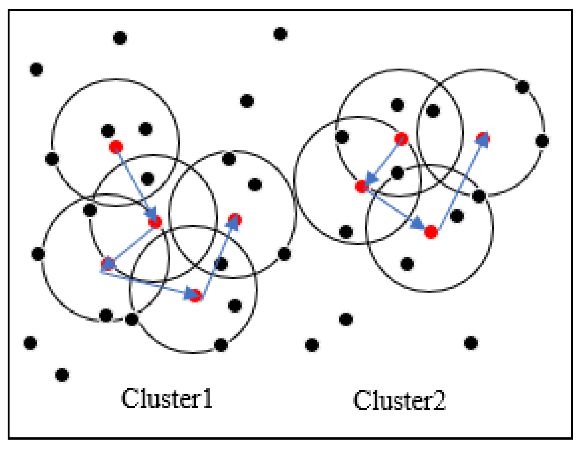
Figure 1 shows the above clustering process of our improved DBSCAN algorithm. MinPts is set to 5 and ε is the radius of the circle in the figure. Red points are core point objects because their ε-neighborhood contains at least five points. Black points are not core point objects. The collection of all the points in the core object ε-neighborhood forms a cluster. In Figure 1, all points in the circle with the blue arrow on the left form one cluster, and all points in the circle with the blue arrow on the right form another cluster. Other points are noise points.

Figure 1.
Clustering process of improved density-based spatial clustering of applications with noise (DBSCAN) algorithm.
2.1.3. Eliminate Noise Points Based on Hough Circle Detection
Point cloud slice D may contain brush point clouds that meet the requirements of core points. The improved DBSCAN clustering algorithm cannot eliminate such points, which will affect the detection accuracy of trunks to some extent. Therefore, Hough circle detection can be performed on the results obtained by the improved DBSCAN clustering algorithm to exclude brush point clouds.
Hough circle detection method uses Hough gradient method to detect circles [30]. In this paper, Hough circle detection was performed three times for each initial clustering result, namely, the point clouds with breast height above and below 10 cm. The detection locations were the point clouds at 10 cm above breast height, the point clouds at breast height and the point clouds at 10 cm below breast height. The clusters that passed Hough circle detection three times are considered to have successfully detected the trunks. Clusters that fail Hough circle detection are considered as brush points. Finally, the clusters that successfully pass Hough circle detection are taken as the initial clustering results.
2.2. Region Growth Layer-by-Layer Clustering
Region growth layer-by-layer clustering is the process of aggregating a group of elements into a larger region [31]. In this paper, the results of trunk detection are used as the initial clustering center. Then, the fuzzy C-means algorithm is used to classify the remaining point clouds. The cluster center obtained at layer i is used as the initial cluster center at layer i + 1 for layer-by-layer clustering until the points in each layer of point clouds are divided.
The fuzzy C-means algorithm is shown in Equation (5), where m is the fuzziness, N is the number of points in this layer, C is the number of clusters, and represents the ith sample with 3D attribute. In addition, represents the membership degree of sample belonging to cluster (Equation (6)). And is the center of cluster (Equation (7)) with 3D attribute. is a measure of Euclidean distance.
Fuzzy C-means algorithm is a process of iteratively calculating the membership degree and cluster center until they reach the optimum. For a single sample , the sum of its membership degree for each cluster is one, as shown in Equation (8).
The termination condition of iteration is shown in Equation (9):
where k is the number of iteration steps and ε is the error threshold. The above formula means that the degree of membership will not change greatly if the iteration continues. That is, the local optimal is achieved.
In the process of clustering with fuzzy C-means method, the initial membership matrix is calculated by the initial clustering center , and the corresponding to the minimum of the objective function is obtained iteratively. Then, the fuzzy membership matrix is calculated by the clustering center . Set the fuzziness m = 2, the number of iterations is 30, and the critical value of iteration ε is 0.0001. Divide each sample data into the corresponding category with the largest membership degree. Set to one layer every 0.5 m. Cluster center obtained at layer i is the initial cluster center of layer i + 1 for layer-by-layer clustering, until the points in each layer of point clouds are divided.
2.3. Materials
2.3.1. Mixed Forests of TLS Point Clouds in Germany
To test the accuracy of individual tree segmentation based on the improved DBSCAN algorithm, we use the TLS point clouds provided by Weiser et al. [32] in the research in 2021 (https://doi.org/10.1594/PANGAEA.933426 (accessed on 1 January 2022)). The datasets are covering some species typical for central European forests. The data collection site is located in the mixed forests of Bretten and Karlsruhe in Baden-Württemberg, southwest Germany. TLS point clouds were captured with a RIEGL VZ-400 (RIEGL LMS GmbH 2017) mounted on a tripod from five to eight static positions per survey, distributed around a selected group of trees. Its accuracy is 5 mm at 100 m scanning range and point density is 7000 points/m3. The pulse repetition rate of the sensor is 300 kHz, the vertical angular step width is 0.017° and the horizontal angular step width is 0.017°. At some positions, an additional scan was performed using a tilt mount, to capture the top of the trees at proximity. Figure 2a shows the TLS point clouds of Plot BR04 collected in July 2019. Figure 2b shows the TLS point clouds of Plot KA09 collected in August 2019.
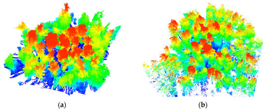
Figure 2.
Terrestrial laser scanning (TLS) data. (a) Plot BR04, (b) Plot KA09.
2.3.2. Artificial Forest of TLS Point Clouds in China
The other experimental data are point clouds of Chinese scholar trees (Sophora japonica) collected by FARO FOCUS150 TLS (FARO Technologies, Inc., www.faro.com (accessed on 1 January 2022)) in the spring of 2018 [33]. The sensor has a horizontal field of view of 360° and a vertical field of view of 300°, with a minimum horizontal and vertical step width of 0.009°. Point density is 4600 points/m3. We adopted the multi-scanning method to obtain a circular block with a radius of 20 m with good vegetation coverage. The circular plot with a radius of 20 m was cut into 4 fan-shaped plots on average (Figure 3). The measured number of trees in each plot was 47, 52, 46 and 33, respectively.

Figure 3.
Original TLS point clouds. Plot 1 (a), Plot 2 (b), Plot 3 (c), Plot 4 (d) are four fan-shaped plots.
2.4. Evaluation Methods
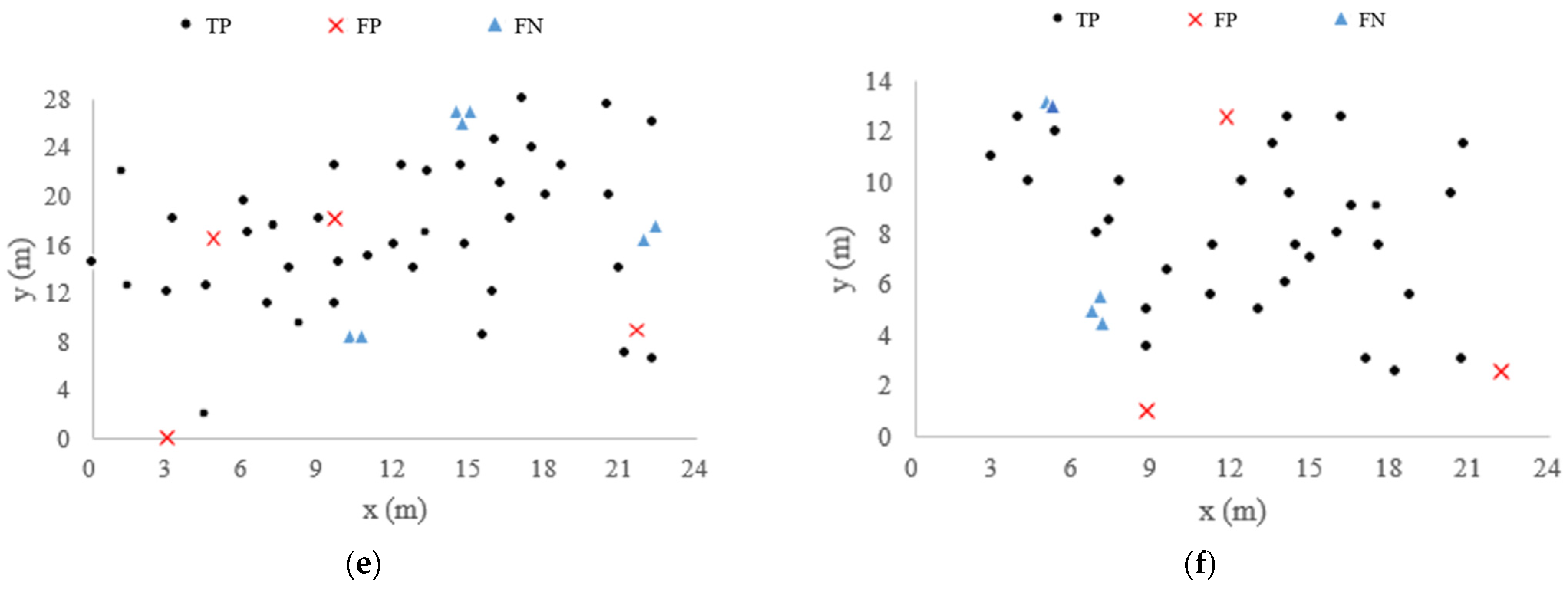
We compared the segmented trees with the reference trees from overall segmentation, trunk detection and small tree segmentation. There are three types in the segmentation results. If a tree is correctly segmented from the TLS data, it is called true positive (TP). If a tree is not split from the TLS data but is assigned to nearby trees, it is called false negative (FN). If a tree does not actually exist but is separated from the point clouds, it is called false positive (FP). TP, FN, and FP represent correct segmentation, under-segmentation, and over-segmentation, respectively. The higher TP value, the lower FN and FP value, the higher accuracy. To evaluate the segmentation method, recall, precision, and F1-score were calculated using the following Equation [28].
Recall represents the percentage of correct segmentation in the actual number. Precision represents the percentage of correct segmentation in the detected number. F1-score comprehensively considers the overall accuracy of under-segmentation and over-segmentation errors. Recall and precision range from 0 to 100%. F1-score ranges from 0 to 1. The higher recall and precision are, the higher F1-score is. If all trees are correctly divided, then recall and precision are equal to 100% and F1-score is equal to 1.
3. Results and Analysis
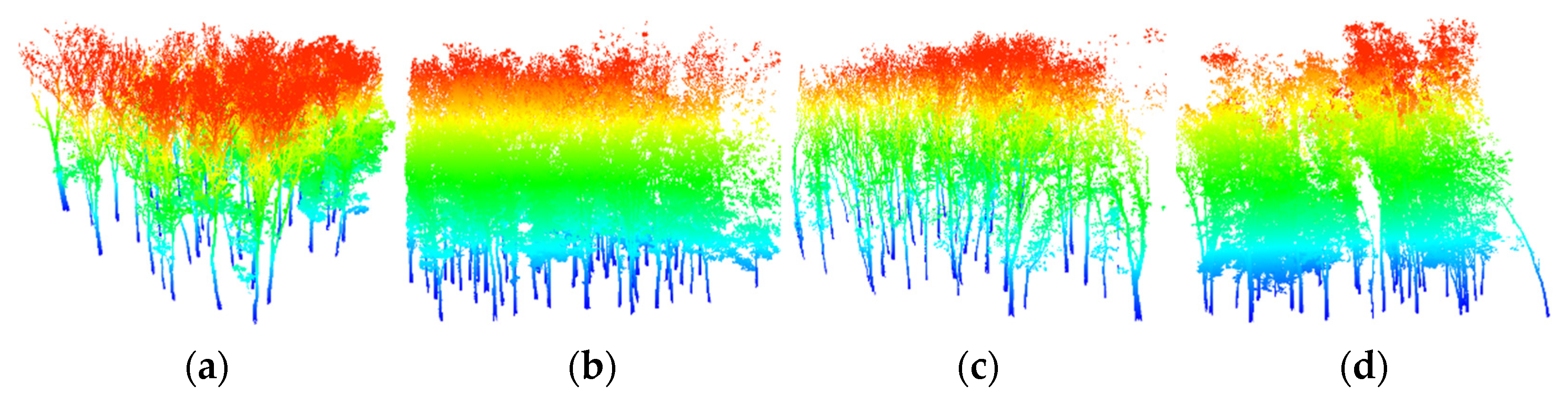
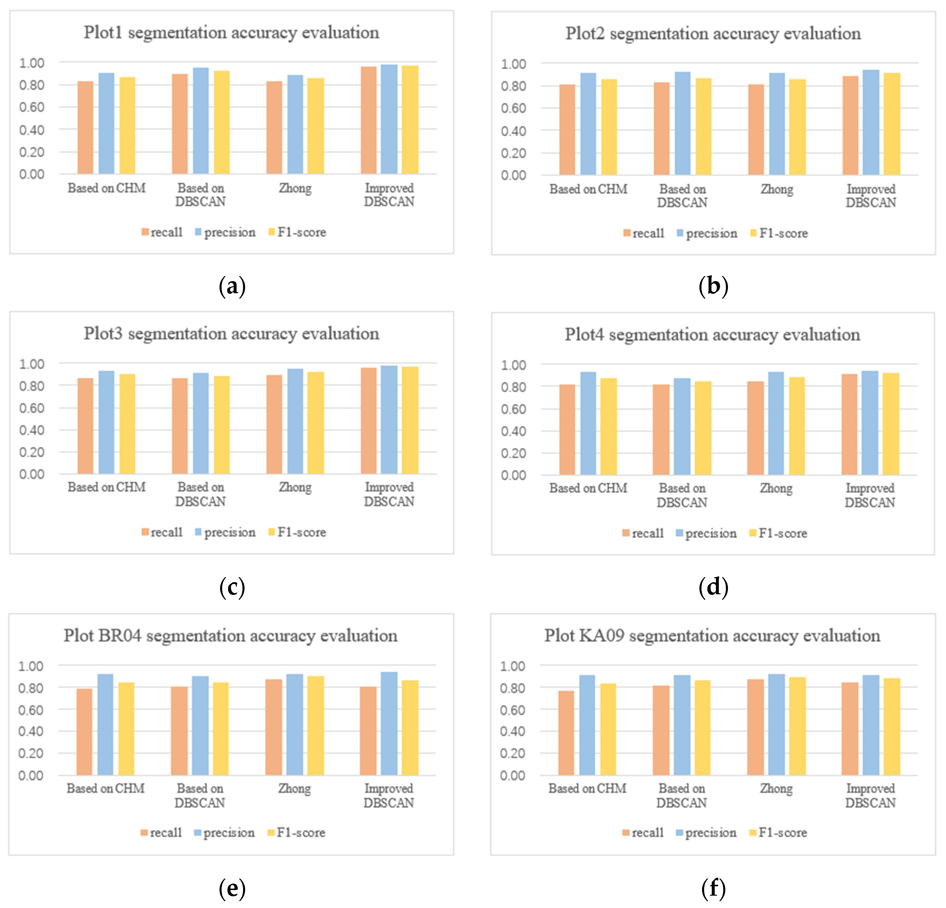
This section explains the results of our individual tree segmentation method from three aspects of overall segmentation results, trunk detection results, and small tree detection results. In addition, we also compared our method with individual tree segmentation methods based on CHM, traditional DBSCAN and Zhong’s method [11]. The segmentation results of the four methods are shown in Figure 4.
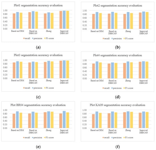
Figure 4.
Results of different segmentation algorithm. The experimental plots include (a) Plot 1, (b) Plot 2, (c) Plot 3, (d) Plot 4, (e) Plot BR04, (f) Plot KA09.
3.1. Results of Individual Tree Segmentation
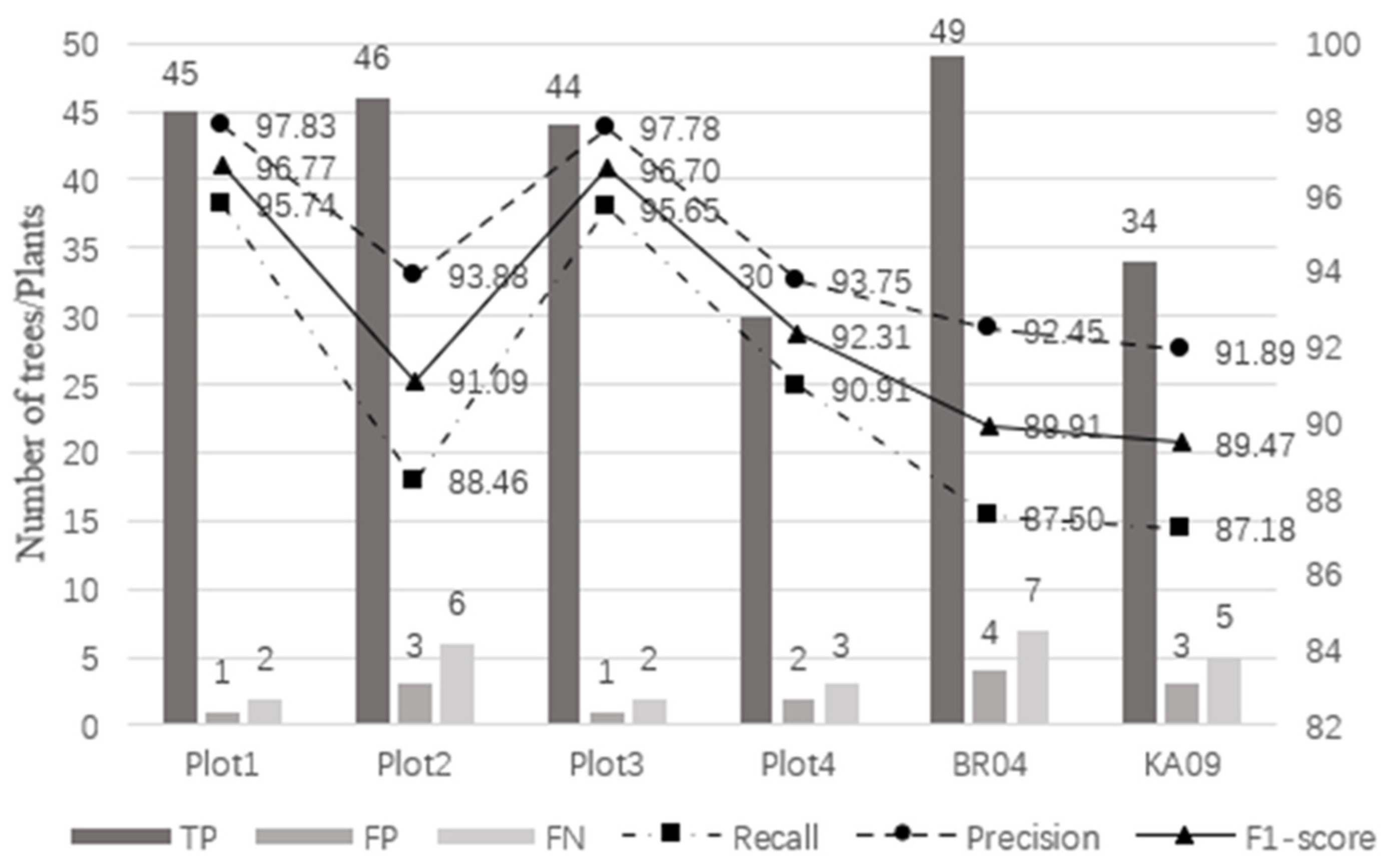
3.1.1. Overall Segmentation Result
Figure 5 shows the individual tree detection results and accuracy of six plots. The total recall, precision, and F1-score of our method in the six plots are 90.84%, 95.38% and 0.93, respectively. The number of trees in Plot 1, Plot 2, Plot 3, and Plot BR04 is similar, while Plot 4 and Plot KA09 have fewer trees. The TP and FN values are added to the number of trees in the actual plot. The recall of individual tree segmentation of the six plots ranges from 87.18% to 95.74%, with a total value of 90.84%. The value of precision varies from 91.89% to 97.83%, with a total value of 95.38%. The value of F1-score varies from 0.89 to 0.97, with a total value of 0.93. Compared with Plot 2 and Plot 4, Plot 1 and Plot 3 have better recall, precision, and F1-score. Compared with the complex forest plot, the recall, precision, and F1-score of the simple forest plot are better. The number of FP in the six plots is lower than that of FN. The number of FN in complex Plot BR04 is seven which is the most. The number of FP in complex Plot BR04 is four, which is the most.
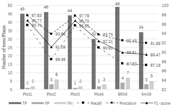
Figure 5.
Individual tree detection results and accuracy of different plot.
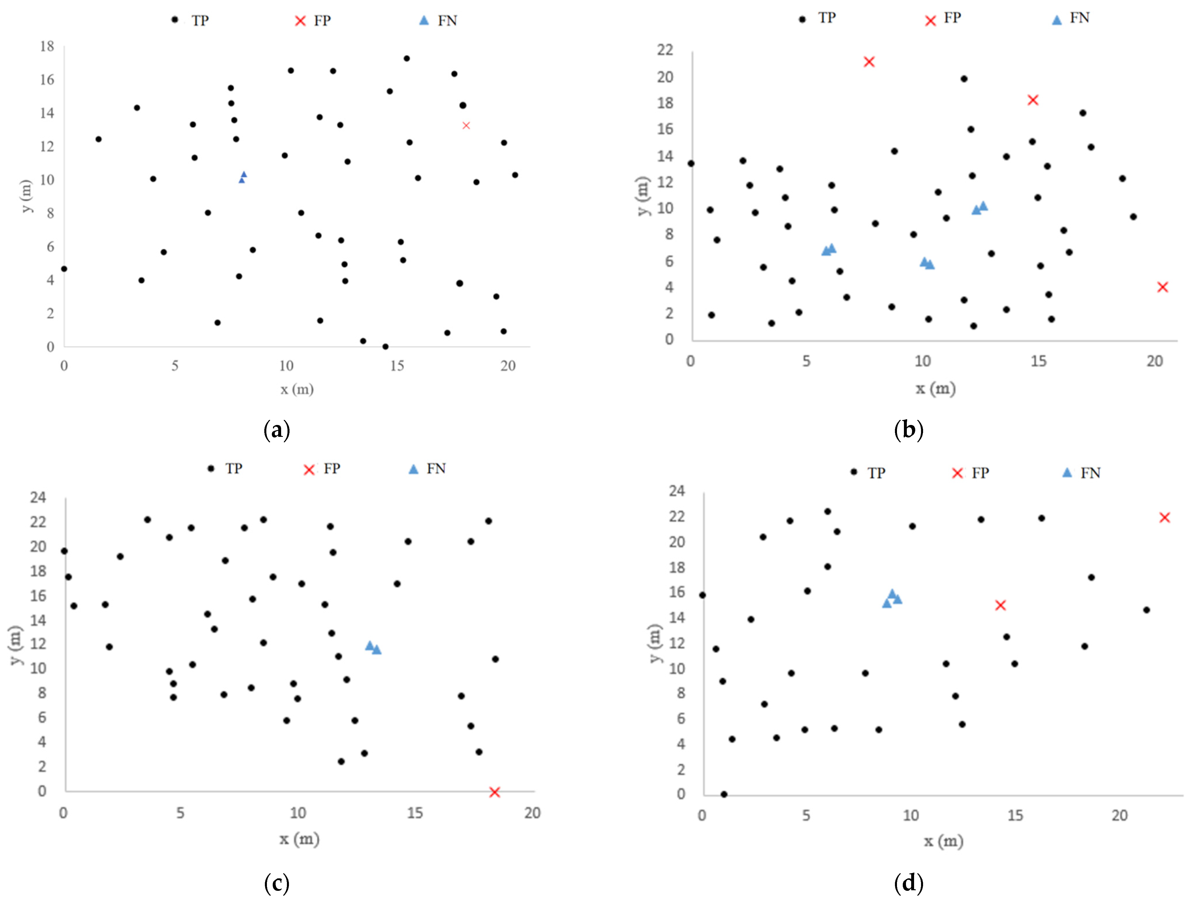
3.1.2. Trunk Detection Results
Figure 6 shows the individual tree segmentation results obtained by using the proposed method, in which the yellow box is the part of the trunk detected after the initial clustering. In order to present the tree detection results of the six plots more vividly, we located the position of each tree by calculating the centroid of the point clouds at the bottom of the tree. TP indicates that the trunk is correctly detected. FP indicates that there is no trunk, but a trunk is detected. FN indicates that there are multiple trunks but only one trunk is detected. The location distribution of the segmentation results of the six plots is shown in Figure 7. A total of 45 trunks are correctly detected in Plot 1. There is a place where the two trunks are identified as one (FP is one). A total of 46 trunks are correctly detected in Plot 2. There are three places where two trunks are identified as one (FP is three). A total of 44 trunks are correctly detected in Plot 3. There is a place where the two trunks are identified as one (FP is one). In Plot 4, 30 trunks are correctly detected. There is a place where three trunks are identified as a single trunk (FP is two). A total of 49 trunks were correctly detected in Plot BR04. There are three places where the multiple trunks are identified as one (FP is four). A total of 34 trunks are correctly detected in Plot KA09. There are two places where the multiple trunks are identified as one (FP is three). As can be seen from the position distribution map, when the distance between the trunks is very close, these trees will be divided into one tree. Additionally, the minimum spacing between segmentation trees is determined by the parameter ε. In conclusion, more than 88% of the trunks could be correctly detected in the six plots, although the trunks are near or far apart from each other.

Figure 6.
Trunk detection results based on improved DBSCAN.
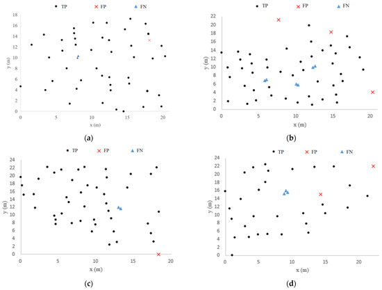
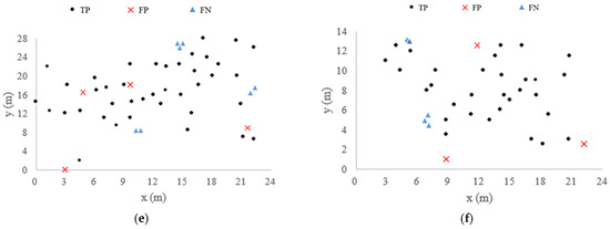
Figure 7.
Individual tree segmentation location distribution map of Plot 1 (a), Plot 2 (b), Plot 3 (c), Plot 4 (d), Plot BR04 (e), Plot KA09 (f).
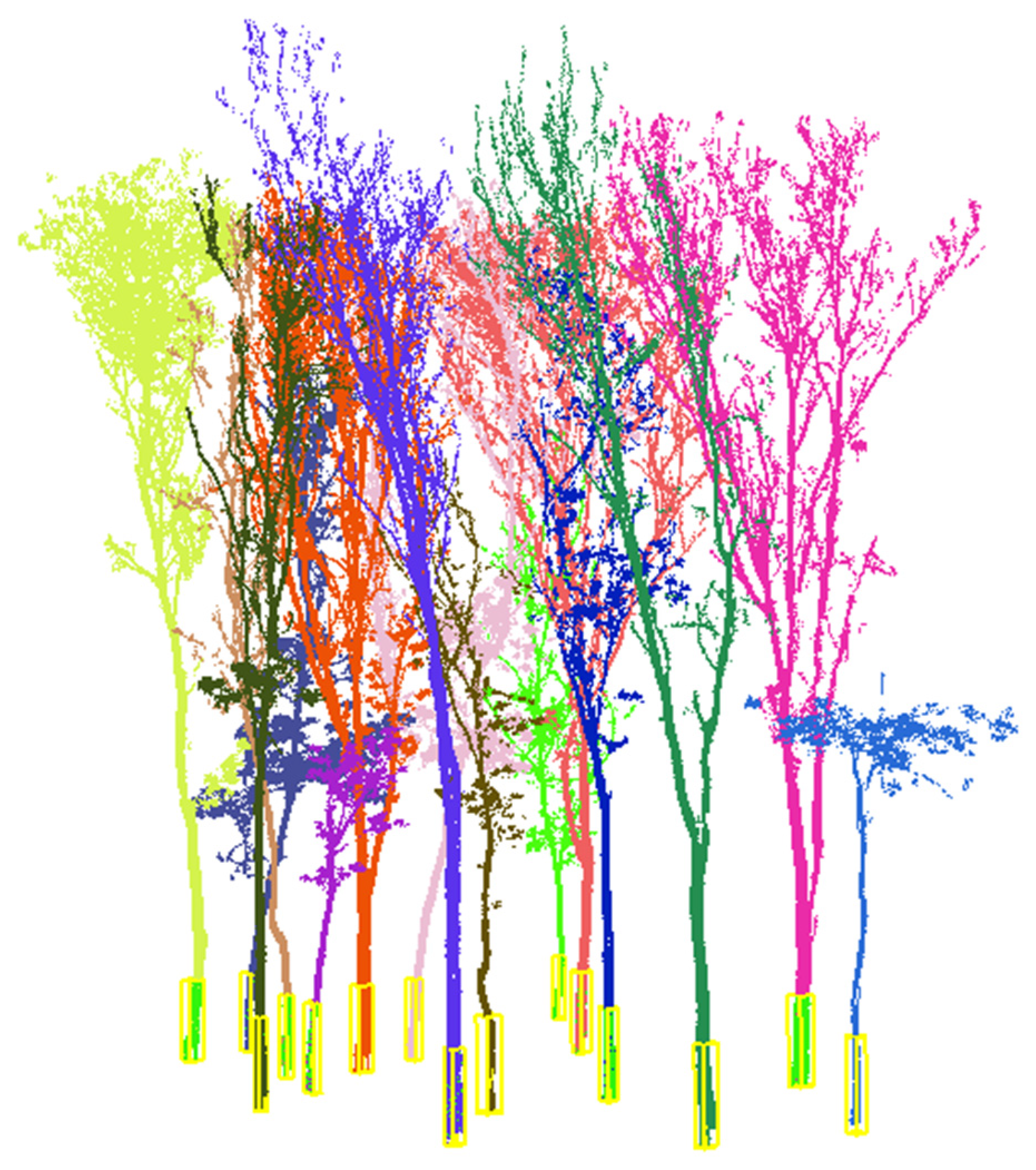
3.1.3. Small Tree Detection Results
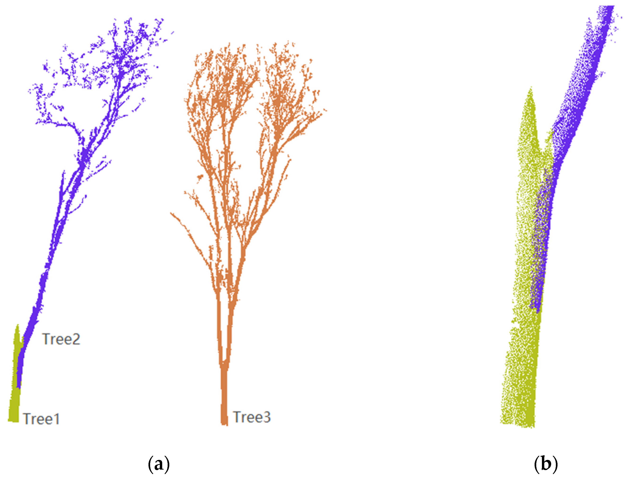
In the segmentation results based on the improved DBSCAN algorithm, there are altogether seven over-segmentation cases, with an error rate of 4.4%. A total of 19, 20 and 22 trees are over-segmented by the other three methods, with an error rate of 7.0%, 7.3% and 8.1%, respectively. There are 25 under-segmentation errors in the segmentation results obtained by our method, with an error rate of 9.2%. There are 273 trees and 93 small trees in the six plots. A total of 77 small trees are correctly identified and segmented, and the correct segmentation rate of small trees reached 82.8%. Figure 8a shows the small light blue tree detected from the TLS point clouds composed of 15 trees, and Figure 8b shows the small purple tree detected.
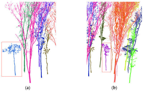
Figure 8.
Segmentation results of small trees under tall trees. (a) The small light blue tree is detected (b) The small purple tree is detected.
3.2. Comparison with Traditional DBSCAN Method
In the segmentation method based on the traditional DBSCAN, the value of recall varies from 80.36% to 89.36%, with a total value of 83.88% (Table 1). The value of precision varies from 87.10% to 95.45%, with a total value of 91.24%. The value of F1-score varies from 0.84 to 0.92, with a total value of 0.87. The recall, precision and F1-score values of Plot 1 are the highest. In this paper, the results of individual tree segmentation based on the improved DBSCAN method is compared with the traditional DBSCAN method. As shown in Figure 4, individual tree segmentation of TLS based on the improved DBSCAN method improves the recall, precision, and F1-score. Compared with the traditional DBSCAN method, the recall, precision, and F1-score in Plot 1 are improved by 6.38%, 2.38% and 0.05, respectively. The recall, precision and F1-score in Plot 2 were improved by 5.77%, 2.39% and 0.04, respectively. In Plot 3, recall, precision, and F1-score are improved by 8.69%, 6.87% and 0.08, respectively. In Plot 4, recall, precision, and F1-score are improved by 9.09%, 4.36% and 0.08, respectively. Compared with the traditional DBSCAN method, the total recall, precision and F1-score of our method are increased by 6.96%, 4.14% and 0.06, respectively.

Table 1.
Segmentation results based on the traditional DBSCAN segmentation method.
3.3. Comparison with CHM Method
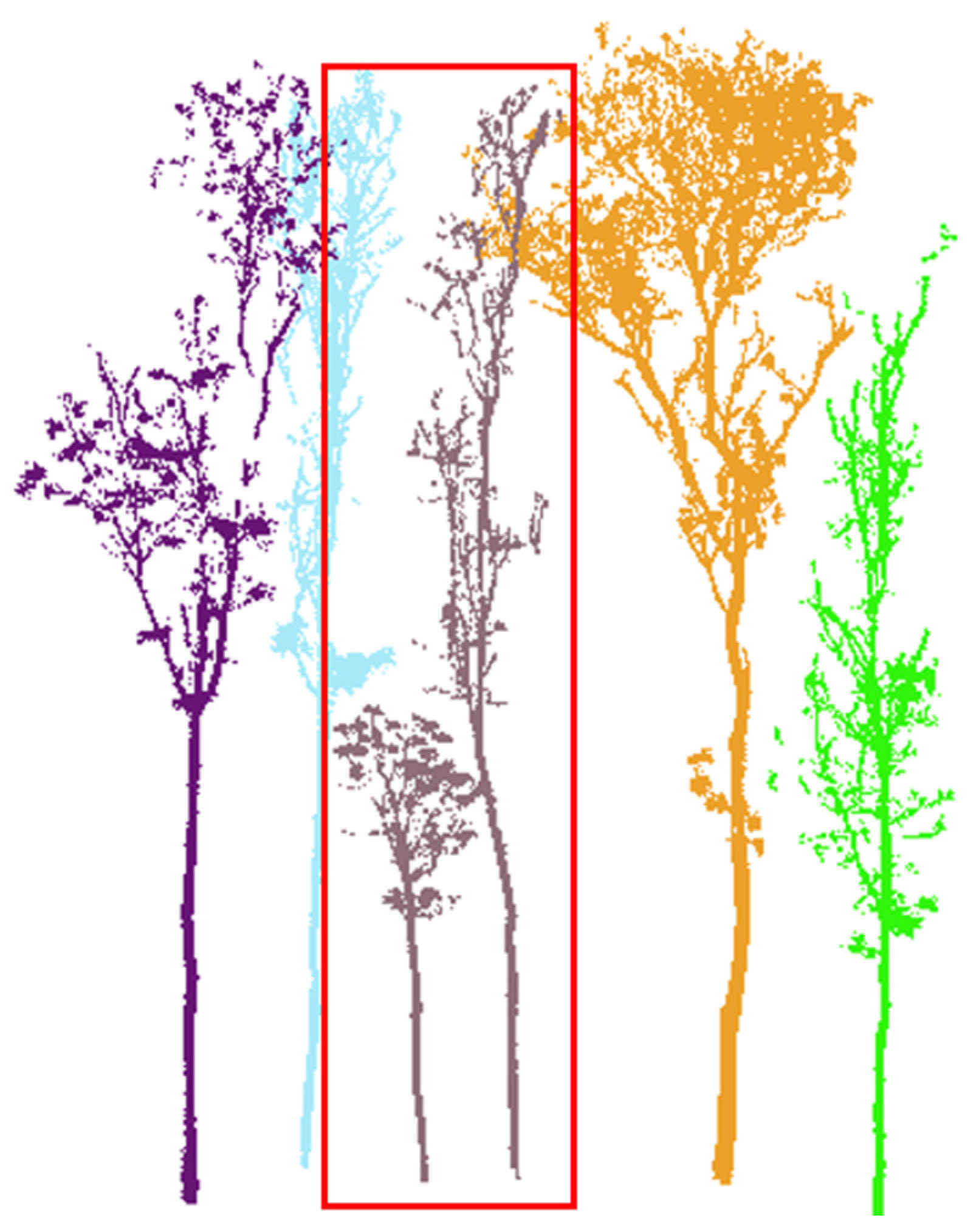
In the CHM-based segmentation method, the value of recall varies from 76.92% to 86.96%, with a total value of 81.32% (Table 2). The value of precision varies from 90.70% to 93.10%, with a total value of 91.74%. The value of F1-score changes from 0.83 to 0.90, with a total value of 0.86. The recall, precision and F1-score values of Plot 3 are the highest. In this paper, the results of individual tree segmentation based on the improved DBSCAN method are compared with the CHM-based method. Individual tree segmentation of TLS based on the improved DBSCAN method improves the results of recall, precision, and F1-score (Figure 4). Compared with the segmentation method based on CHM, the total recall, precision, and F1-score of our method improved by 9.52%, 3.64% and 0.07, respectively. The individual tree segmentation method based on CHM has difficultly detecting small trees under tall tree crowns, especially when small trees are completely blocked. The distance between the breast height of small tree and tall tree in the red box in Figure 9 is 1.09 m, which is much larger than the ε value of the proposed method in Plot 4 of 0.78 m. However, the small tree in the red box is not correctly detected by the CHM-based segmentation (Figure 9).
Table 2.
Segmentation results based on the CHM segmentation method.

Figure 9.
Small tree in the red box is not detected based on CHM segmentation method (the distance between the breast height of the two trees in the red box is 1.09 m).
3.4. Comparison with Zhong’s Method
In the individual tree segmentation method of Zhong et al. [11], the value of recall varies from 80.36% to 89.13%, with a total value of 83.52% (Table 3). The value of precision varies from 88.64% to 95.35%, with a total value of 92.31%. The value of F1-score changes from 0.86 to 0.92, with a total value of 0.88. In this paper, the results of individual tree segmentation based on the improved DBSCAN method are compared with the segmentation method of Zhong et al. [11]. As shown in Figure 4, individual tree segmentation of TLS based on the improved DBSCAN method improves the results of recall, precision, and F1-score. Compared with Zhong’s method, the total recall, precision, and F1-score of our method are improved by 7.32%, 3.07% and 0.05, respectively. Like the individual tree segmentation method based on CHM, the detection effect of small trees under tall trees is poor. The segmentation errors of small trees account for 77.8% of under segmentation.
Table 3.
Segmentation results based on Zhong’s segmentation method.
4. Discussion
4.1. Optimization Verification of Parameters Automatically Obtained
Comesana-cebral et al. [24] proposed an individual tree segmentation method based on iterative DBSCAN cylinder volume clustering analysis, requiring manual input of two parameters ε and MinPts. If the value of ε is set very small, a large portion of the data set will not be clustered into meaningful clusters but will be treated as outliers because it does not satisfy the number of points within a particular region to define a dense region. If the ε value is set too high, most of the valuable and meaningless data will be merged into the same cluster. If the number of points in the cluster is greater than or equal to MinPts, then these points are considered part of the cluster. If the number of points in the cluster is less than MinPts, then these points are considered noise points or outliers. Our improved DBSCAN method can automatically obtain the optimal parameters ε and MinPts. The choice of these two parameters will affect the result of the trunk detection. The result of trunk detection is related to the number of trees. During the experiment, N groups of parameters ε and MinPts are successively taken as the input parameters of the DBSCAN algorithm to obtain the cluster number corresponding to each group of parameters. If there is no change in the number of clusters obtained by continuous multiple groups of parameters, the group of parameters is considered to have the best adaptability.
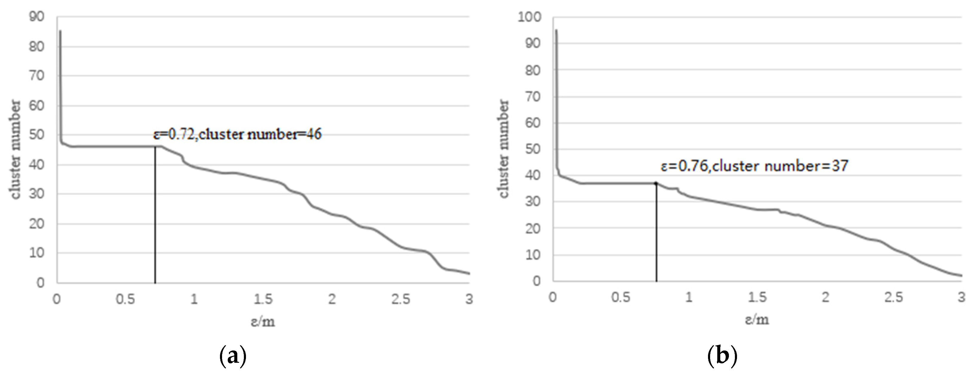
The automatically obtained ε is 0.72 and MinPts is 9 in Plot 1. When ε is in the range of 0.2 to 0.75, the cluster number does not change (Figure 10a). Therefore, the obtained parameters are the optimal values in Plot 1. The automatically obtained ε is 0.76 and is 15 in Plot KA09. When ε is in the range of 0.25 to 0.76, the cluster number does not change (Figure 10b). Therefore, the obtained parameters are the optimal values in Plot KA09. When ε is small, the cluster number is large, and there will be more over-segmentation errors in the segmentation results (Figure 11). In the layer-by-layer clustering process of regional growth, the wrong trunks are assigned the remaining point clouds, which is meaningless to the wrong trees. When ε is large, the cluster number is small, and there will be more under-segmentation errors in the segmentation results (Figure 12). Because the value of ε is set too large, the trunk detection method considers that these point clouds belong to the same trunk and fails to segment them correctly. Finally, the result of individual tree segmentation is to allocate the point clouds of multiple trees to one tree. So when the cluster number does not change, the over-segmentation and under-segmentation errors in the segmentation result are the least.
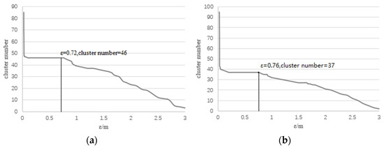
Figure 10.
The relationship between ε and cluster number. Plot 1: The optimal ε is 0.72, MinPts is 9 according to Equation (4). KA09: The optimal ε is 0.76, MinPts is 15. (a) When ε is in the range of 0.2 to 0.75, the cluster number does not change. (b) When ε is in the range of 0.25 to 0.76, the cluster number does not change.
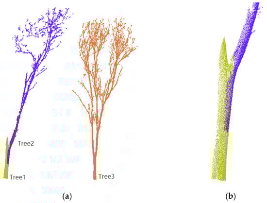
Figure 11.
Over-segmentation error. (a) when ε = 0.02 (<0.72), a tree was wrongly divided into two trees Tree1 and Tree2. (b) Partial enlargement of Tree1 and Tree2.
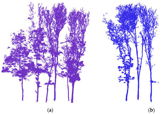
Figure 12.
Under-segmentation error. When ε = 3 (>0.72), (a) six trees are not correctly segmented, (b) three trees are not correctly segmented.
The results show that the parameters obtained automatically by the proposed method are optimal in artificial forest and mixed forest. In future research, we will automatically generate the corresponding ε of the tree according to the different distances between adjacent trees in the sample plot to further improve the segmentation accuracy.
4.2. Analysis of Small Tree Detection Results
There are 273 trees in the six plots, including 93 small trees. Among the segmentation results based on our method, 25 trees are over-segmented, with an error rate of 9.2%. In the other three methods, 51, 44 and 45 trees are over-segmented, with error rates of 18.7%, 16.1% and 16.5%, respectively. The number of under-segmented trees in method proposed by Zhong et al. [11] is 45, among which 35 small trees are unsegmented. The results show that these three comparison methods are easy to miss small trees under tall trees, while our method can greatly improve the detection ability of small trees. Our method has a great improvement in reducing the errors of over-segmentation and under-segmentation. Especially for the reduction in under-segmentation errors, the improvement is more than doubled. This is because our method can greatly improve the identification of small trees under tall tree crowns.
4.3. Individual Tree Segmentation Analysis of Complex Forest
In the mixed forest, the recall, precision, and F1-score of segmentation are 87.37%, 94.32% and 0.91, respectively. While in the artificial forest, the recall, precision, and F1-score of segmentation are 92.70%, 95.93% and 0.94, respectively. The segmentation effect is better for simple forest types, and relatively poor for individual tree segmentation of forked trees, multi-trunk trees and other complex trees. Because in the result of segmentation, the trunk that belongs to one tree may be mistaken for multiple trees, resulting in the phenomenon of false segmentation. In the case of more complex trunks, the choice of parameters ε and is more important. However, the appropriate parameter ε can still bring the point clouds at the trunk together. When the distance between multiple trunks belonging to the same tree is much smaller than the distance between different trees, the improved DBSCAN algorithm will obtain the appropriate value of the parameter ε, so our method can achieve good segmentation effect in this case. However, the total segmentation effect is not as good as the simple case of individual trunk. Figure 13 shows an example of partially complex tree segmentation.
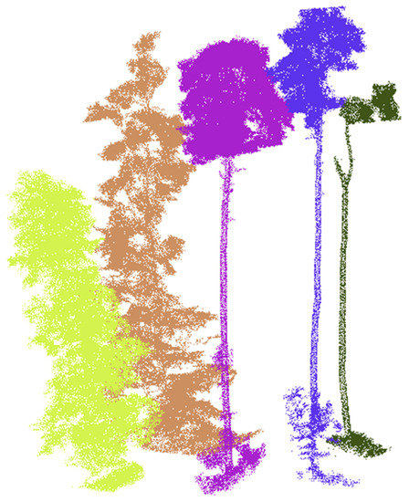
Figure 13.
Partial complex tree segmentation results.
5. Conclusions
We proposed an improved DBSCAN which can automatically determine the optimal cluster number and corresponding input parameters based on DDM and applied the method to segment individual tree from TLS point cloud. This method makes full use of the characteristic of natural separation between trunks and achieves good results in tree segmentation. In addition, we use TLS data of Chinese artificial forest and German mixed forest to evaluate the efficiency of the method. The results show that the method improves the detection of small trees under tall trees and reduces the error of under-segmentation and over-segmentation. By comparing three existing methods, the proposed method can achieve high segmentation accuracy and segment the trunk from the point cloud without missing the details of the crown. This study lays a foundation for the calculation and fine modeling of tree height, DBH, biomass and other parameters based on TLS point clouds.
Author Contributions
Conceptualization, H.F. and H.L.; methodology, H.L. and Y.D.; software, H.L. and Y.D.; validation, H.F., H.L. and Y.D.; formal analysis, H.L.; investigation, H.L.; resources, H.L.; data curation, Y.D.; writing—original draft preparation, H.F. and H.L.; writing—review and editing, H.L., Y.D. and F.C.; visualization, Y.D.; supervision, F.C. and F.X.; project administration, F.C. and F.X.; funding acquisition, F.X. All authors have read and agreed to the published version of the manuscript.
Funding
This research was funded by Focus Tracking Project of Beijing Forestry University (No. BLRD202124) and National Natural Science Foundation of China (No.61772078).
Data Availability Statement
Not applicable.
Conflicts of Interest
The authors declare no conflict of interest.
Appendix A
Firstly, obtain the point cloud slice at the top and bottom 10 cm of the breast height after point clouds preprocessing, and initialize the core point object . Then, starting from any point in point cloud slice , find the set of points in point cloud slice (including point itself). Satisfy that the Euclidean distance between point and any other point in point cloud slice is less than or equal to . Record the set of points as , that is, the neighborhood sample set of point (Equation (A1)):
Secondly, if there are enough points in the ε neighborhood sample set of point , and the number is greater than or equal to (Equation (A2)). Then, point is marked as the core point and add the point to the core point object set . Repeat the above steps for the remaining points in point cloud slice , and constantly update the core point object set until all the core points in point cloud slice are found.
Thirdly, initialize the cluster number k = 0 and the unvisited sample set τ. Record the current visited sample set .
Fourth, select a core point object from the core point object set randomly, and initialize the queue . (1) Take the first sample in queue . If the number of points in the neighborhood of sample is greater than or equal to MinPts, then set , and add the sample in Δ to queue , then set . (2) Next, take the next sample from the queue , repeat process (1) in step 4 to calculate the number of points in the ε neighborhood of sample q and subsequent operations, until all samples in queue are calculated. When queue is empty, that is, all the samples in queue are calculated, then set k = k + 1 and a new cluster is formed. Record the new cluster as , update the core point object set at the same time. (3) Finally, repeat the whole process of (1) and (2) in step 4 until the core point object set is empty. The final clusters represent the initial clustering results of trunk detection.
References
- Cabo, C.; Ordóñez, C.; López-Sánchez, C.A.; Armesto, J. Automatic dendrometry: Tree detection, tree height and diameter estimation using terrestrial laser scanning. Int. J. Appl. Earth Obs. Geoinf. 2018, 69, 164–174. [Google Scholar] [CrossRef]
- Chen, W.; Xiang, H.B.; Moriya, K. Individual Tree Position Extraction and Structural Parameter Retrieval Based on Airborne LiDAR Data: Performance Evaluation and Comparison of Four Algorithms. Remote Sens. 2020, 12, 571. [Google Scholar] [CrossRef] [Green Version]
- Rudge, M.L.M.; Levick, S.R.; Bartolo, R.E.; Erskine, P.D. Modelling the Diameter Distribution of Savanna Trees with Drone-Based LiDAR. Remote Sens. 2021, 13, 1266. [Google Scholar] [CrossRef]
- Fan, G.; Nan, L.; Dong, Y.; Su, X.; Chen, F. AdQSM: A New Method for Estimating Above-Ground Biomass from TLS Point Clouds. Remote Sens. 2020, 12, 3089. [Google Scholar] [CrossRef]
- Zheng, Y.; Jia, W.; Wang, Q.; Huang, X. Deriving Individual-Tree Biomass from Effective Crown Data Generated by Terrestrial Laser Scanning. Remote Sens. 2019, 11, 2793. [Google Scholar] [CrossRef] [Green Version]
- Yu, R.; Luo, Y.; Zhou, Q.; Zhang, X.; Wu, D.; Ren, L. A machine learning algorithm to detect pine wilt disease using UAV-based hyperspectral imagery and LiDAR data at the tree level. Int. J. Appl. Earth Obs. Geoinf. 2021, 101, 102363. [Google Scholar] [CrossRef]
- Yang, J.; Kang, Z.; Cheng, S.; Yang, Z.; Akwensi, P.H. An individual tree segmentation method based on watershed algorithm and three-dimensional spatial distribution analysis from airborne LiDAR point clouds. IEEE J. Sel. Top. Appl. Earth Obs. Remote Sens. 2020, 13, 1055–1067. [Google Scholar] [CrossRef]
- Disney, M.I.; Boni Vicari, M.; Burt, A.; Calders, K.; Lewis, S.L.; Raumonen, P.; Wilkes, P. Weighing trees with lasers: Advances, challenges and opportunities. Interface Focus. 2018, 8, 20170048. [Google Scholar] [CrossRef] [Green Version]
- Xu, D.; Wang, H.; Xu, W.; Luan, Z.; Xu, X. LiDAR Applications to Estimate Forest Biomass at Individual Tree Scale: Opportunities, Challenges and Future Perspectives. Forests 2021, 12, 550. [Google Scholar] [CrossRef]
- Liang, X.; Hyyppä, J.; Kaartinen, H.; Lehtomäki, M.; Pyörälä, J.; Pfeifer, N.; Wang, Y. International benchmarking of terrestrial laser scanning approaches for forest inventories. ISPRS J. Photogramm. Remote Sens. 2018, 144, 137–179. [Google Scholar] [CrossRef]
- Zhong, L.; Cheng, L.; Xu, H.; Chen, Y.; Li, M. Segmentation of individual trees from TLS and MLS data. IEEE J. Sel. Top. Appl. Earth Obs. Remote Sens. 2016, 10, 774–787. [Google Scholar] [CrossRef]
- Hillman, S.; Wallace, L.; Reinke, K.; Jones, S. A comparison between TLS and UAS LiDAR to represent eucalypt crown fuel characteristics. ISPRS J. Photogramm. Remote Sens. 2021, 181, 295–307. [Google Scholar] [CrossRef]
- Tao, S.; Wu, F.; Guo, Q.; Wang, Y.; Li, W. Segmenting tree crowns from terrestrial and mobile LiDAR data by exploring ecological theories. ISPRS J. Photogramm. Remote Sens. 2015, 110, 66–76. [Google Scholar] [CrossRef] [Green Version]
- Paris, C.; Kelbe, D.; Van Aardt, J.; Bruzzone, L. A novel automatic method for the fusion of ALS and TLS LiDAR data for robust assessment of tree crown structure. IEEE Trans. Geosci. Remote Sens. 2017, 55, 3679–3693. [Google Scholar] [CrossRef]
- Lu, X.; Guo, Q.; Li, W.; Flanagan, J. A bottom-up approach to segment individual deciduous trees using leaf-off lidar point cloud data. ISPRS J. Photogramm. Remote Sens. 2014, 94, 1–12. [Google Scholar] [CrossRef]
- Ayrey, E.; Fraver, S.; Kershaw, J.A., Jr.; Kenefic, L.S.; Hayes, D.; Weiskittel, A.R.; Roth, B.E. Layer Stacking: A Novel Algorithm for Individual Forest Tree Segmentation from LiDAR Point Clouds. Can. J. Remote Sens. 2017, 43, 16–27. [Google Scholar] [CrossRef]
- Khosravipour, A.; Skidmore, A.K.; Isenburg, M.; Wang, T.; Hussin, Y.A. Generating Pit-free Canopy Height Models from Airborne Lidar. Photogramm. Eng. Remote Sens. 2014, 80, 863–872. [Google Scholar] [CrossRef]
- Morsdorf, F.; Meier, E.; Kötz, B.; Itten, K.I.; Dobbertin, M.; Allgower, B. LIDAR-based geometric reconstruction of boreal type forest stands at single tree level for forest and wildland fire management. Remote Sens. Environ. 2004, 92, 353–362. [Google Scholar] [CrossRef]
- Jakubowski, M.; Li, W.; Guo, Q.; Kelly, M. Delineating individual trees from LiDAR data: A comparison of vector-and raster-based segmentation approaches. Remote Sens. 2013, 5, 4163–4186. [Google Scholar] [CrossRef] [Green Version]
- Yang, Q.; Su, Y.; Jin, S.; Kelly, M.; Hu, T.; Ma, Q.; Li, Y.; Song, S.; Zhang, J.; Xu, G.; et al. The Influence of Vegetation Characteristics on Individual Tree Segmentation Methods with Airborne LiDAR Data. Remote Sens. 2019, 11, 2880. [Google Scholar] [CrossRef] [Green Version]
- Wu, B.; Yu, B.; Yue, W.; Shu, S.; Tan, W.; Hu, C.; Huang, Y.; Wu, J.; Liu, H. A voxel-based method for automated identification and morphological parameters estimation of individual street trees from mobile laser scanning data. Remote Sens. 2013, 5, 584–611. [Google Scholar] [CrossRef] [Green Version]
- Lee, H.; Slatton, K.C.; Roth, B.E.; Cropper, W.P. Adaptive clustering of airborne LiDAR data to segment individual tree crowns in managed pine forests. Int. J. Remote Sens. 2010, 31, 117–139. [Google Scholar] [CrossRef]
- Xing, W.; Xing, Y.; Huang, Y.; Qu, L.; You, H. Individual tree segmentation of TLS point cloud data based on clustering of voxels layer by layer. J. Cent. South Univ. For. Technol. 2017, 37, 58–64. [Google Scholar]
- Comesaña-Cebral, L.; Martínez-Sánchez, J.; Lorenzo, H.; Arias, P. Individual Tree Segmentation Method Based on Mobile Backpack LiDAR Point Clouds. Sensors 2021, 21, 6007. [Google Scholar] [CrossRef] [PubMed]
- Nguyen, H.T.; Lee, E.; Bae, C.H.; Lee, S. Multiple Object Detection Based on Clustering and Deep Learning Methods. Sensors 2020, 20, 4424. [Google Scholar] [CrossRef]
- Kim, J.; Choi, J.; Yoo, K.; Nasridinov, A. AA-DBSCAN: An approximate adaptive DBSCAN for finding clusters with varying densities. J. Supercomput. 2019, 75, 142–169. [Google Scholar] [CrossRef]
- Chen, X.; Xi, Q. Research and Implementation of Adaptive Clustering Algorithm based on DBSCAN. J. Huaiyin Teach. Coll. 2021, 20, 228–234. [Google Scholar]
- Li, W.; Yan, S.; Jiang, Y.; Zhang, S.; Wang, C. Research on Method of Self-Adaptive Determination of DBSCAN Algorithm Parameters. Comput. Eng. Appl. 2019, 55, 1–7. [Google Scholar]
- Chen, Q.; Wang, X.; Hang, M.; Li, J. Research on the improvement of single tree segmentation algorithm based on airborne LiDAR point cloud. Open Geosci. 2021, 13, 705–716. [Google Scholar] [CrossRef]
- Feng, J.; Li, Z.; Rong, Y.; Sun, Z. Identification of mature tomatoes based on an algorithm of modified circle Hough transform. J. Chin. Agric. Mech. 2021, 42, 190–196. [Google Scholar]
- Li, W.; Guo, Q.; Jakubowski, M.K.; Kelly, M. A New Method for Segmenting Individual Trees from the Lidar Point Cloud. Photogramm. Eng. Remote Sens. 2012, 78, 75–84. [Google Scholar] [CrossRef] [Green Version]
- Weiser, H.; Schäfer, J.; Winiwarter, L. Terrestrial, UAV-borne, and airborne laser scanning point clouds of central European forest plots, Germany, with extracted individual trees and manual forest inventory measurements. PANGAEA 2021. [Google Scholar] [CrossRef]
- Fan, G.; Nan, L.; Chen, F.; Dong, Y.; Wang, Z.; Li, H.; Chen, D. A new quantitative approach to tree attributes estimation based on LiDAR point clouds. Remote Sens. 2020, 12, 1779. [Google Scholar] [CrossRef]


Publisher’s Note: MDPI stays neutral with regard to jurisdictional claims in published maps and institutional affiliations. |
© 2022 by the authors. Licensee MDPI, Basel, Switzerland. This article is an open access article distributed under the terms and conditions of the Creative Commons Attribution (CC BY) license (https://creativecommons.org/licenses/by/4.0/).