
LiDAR as a Tool for Assessing Change in Vertical Fuel Continuity Following Restoration


Abstract
:1. Introduction
2. Materials and Methods
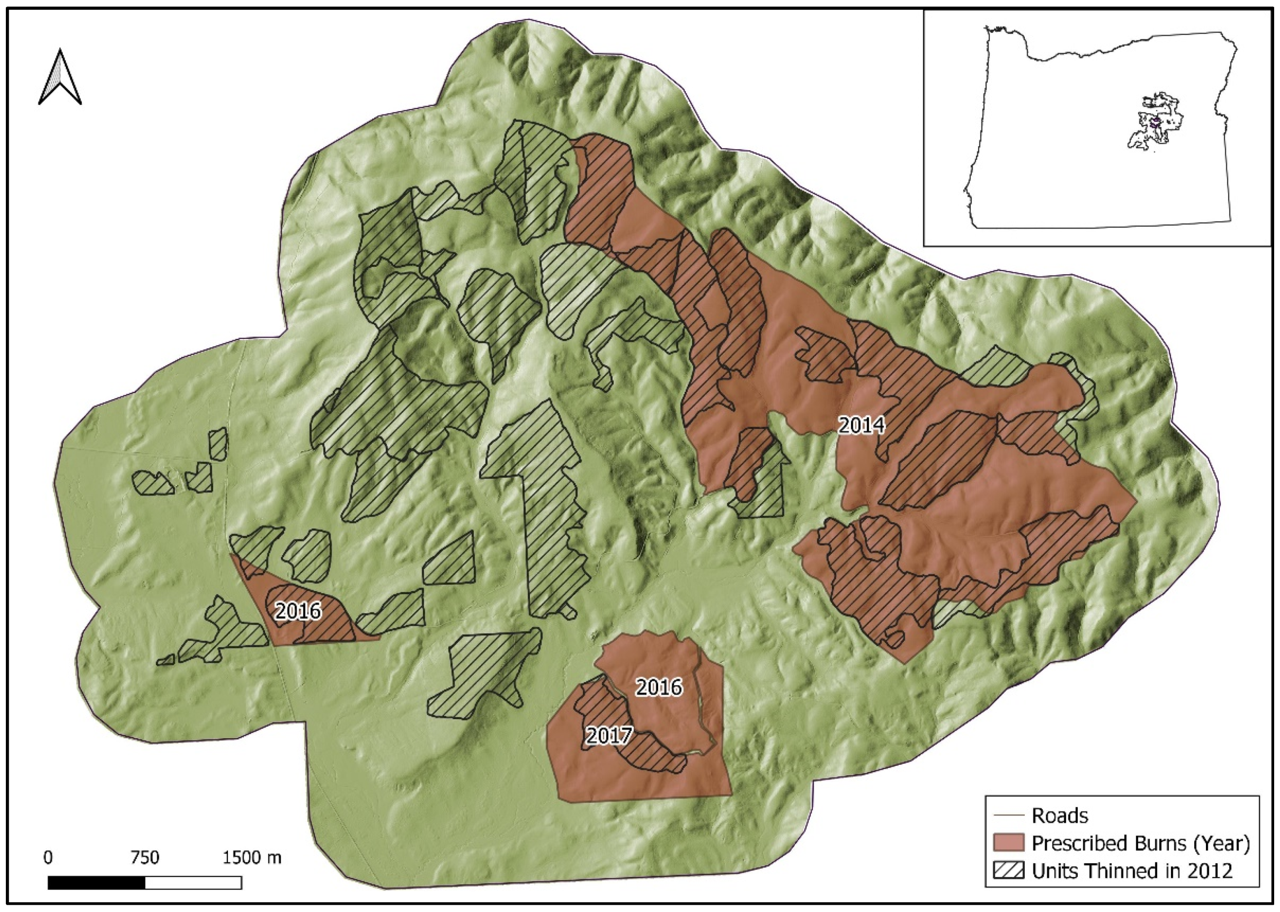
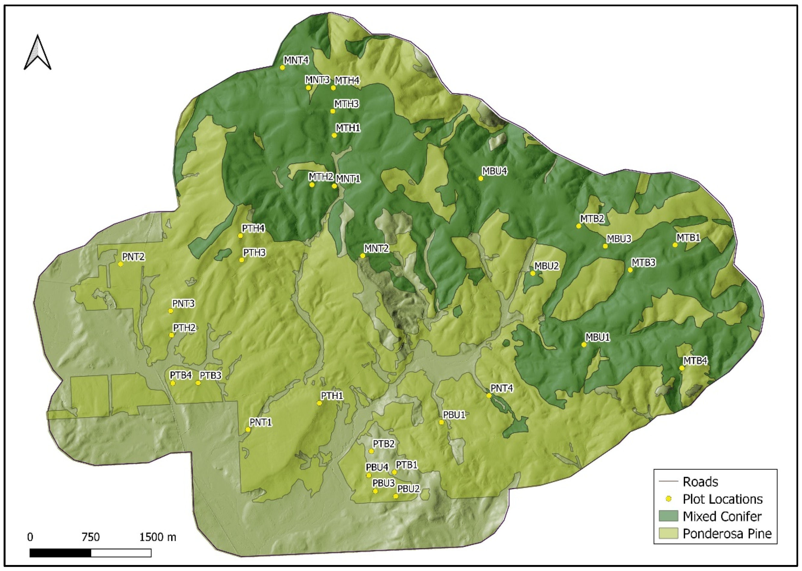
2.1. Study Area
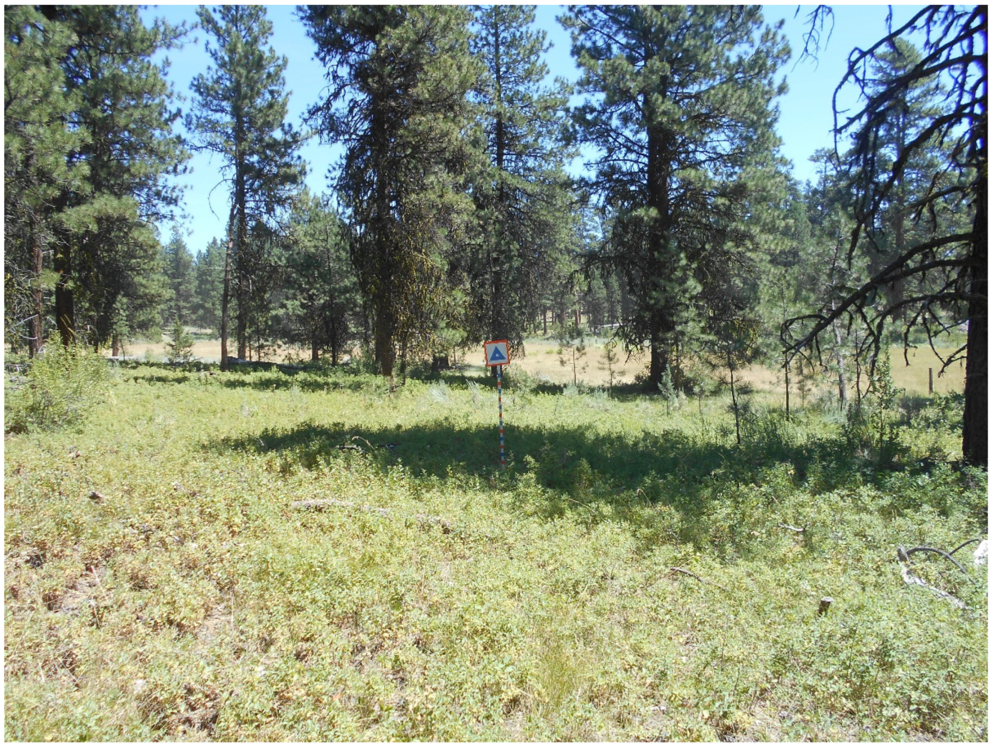
2.2. Field Data
2.3. LiDAR Data Collection and Processing
2.4. Data Analysis
2.5. Sample Units
3. Results
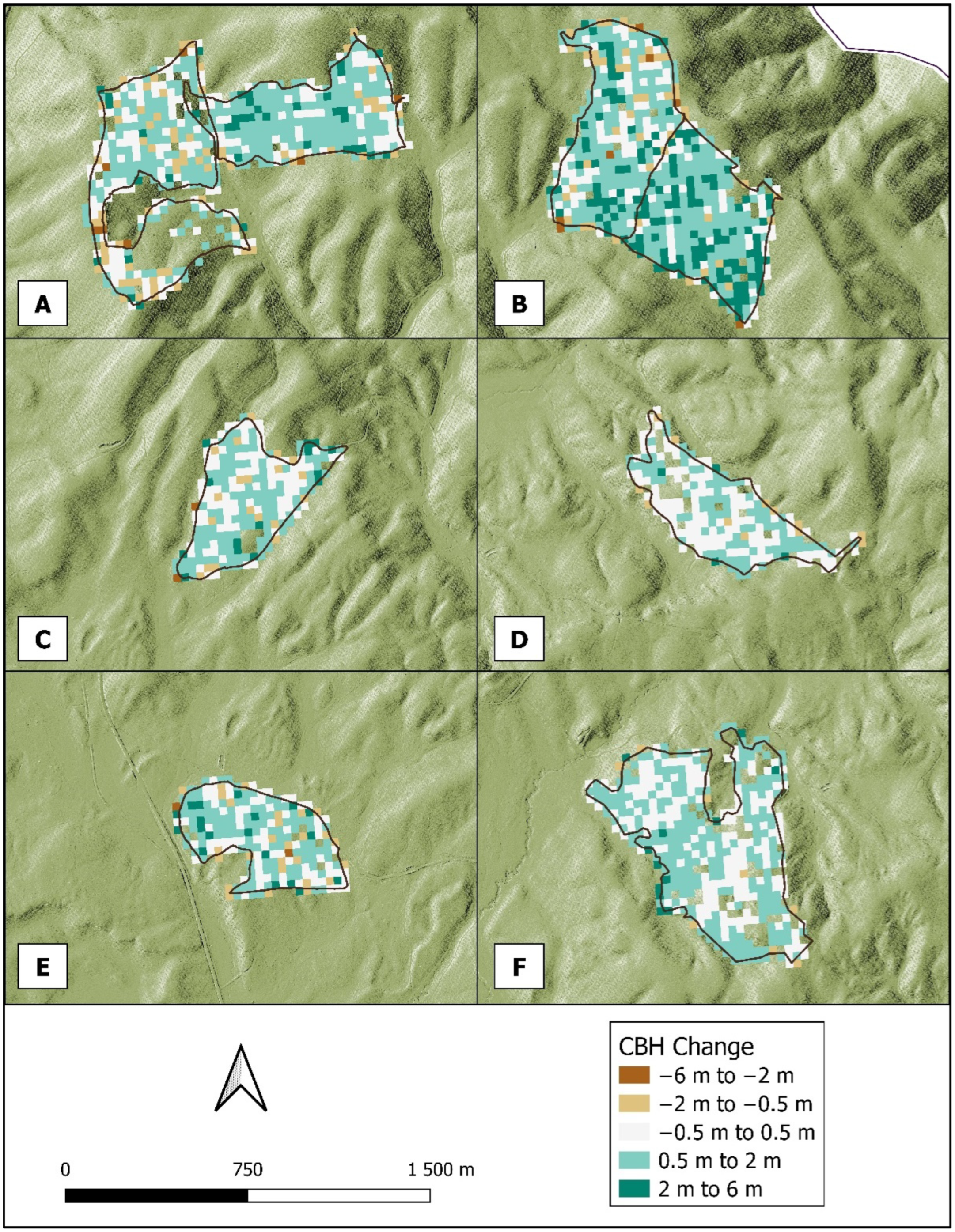
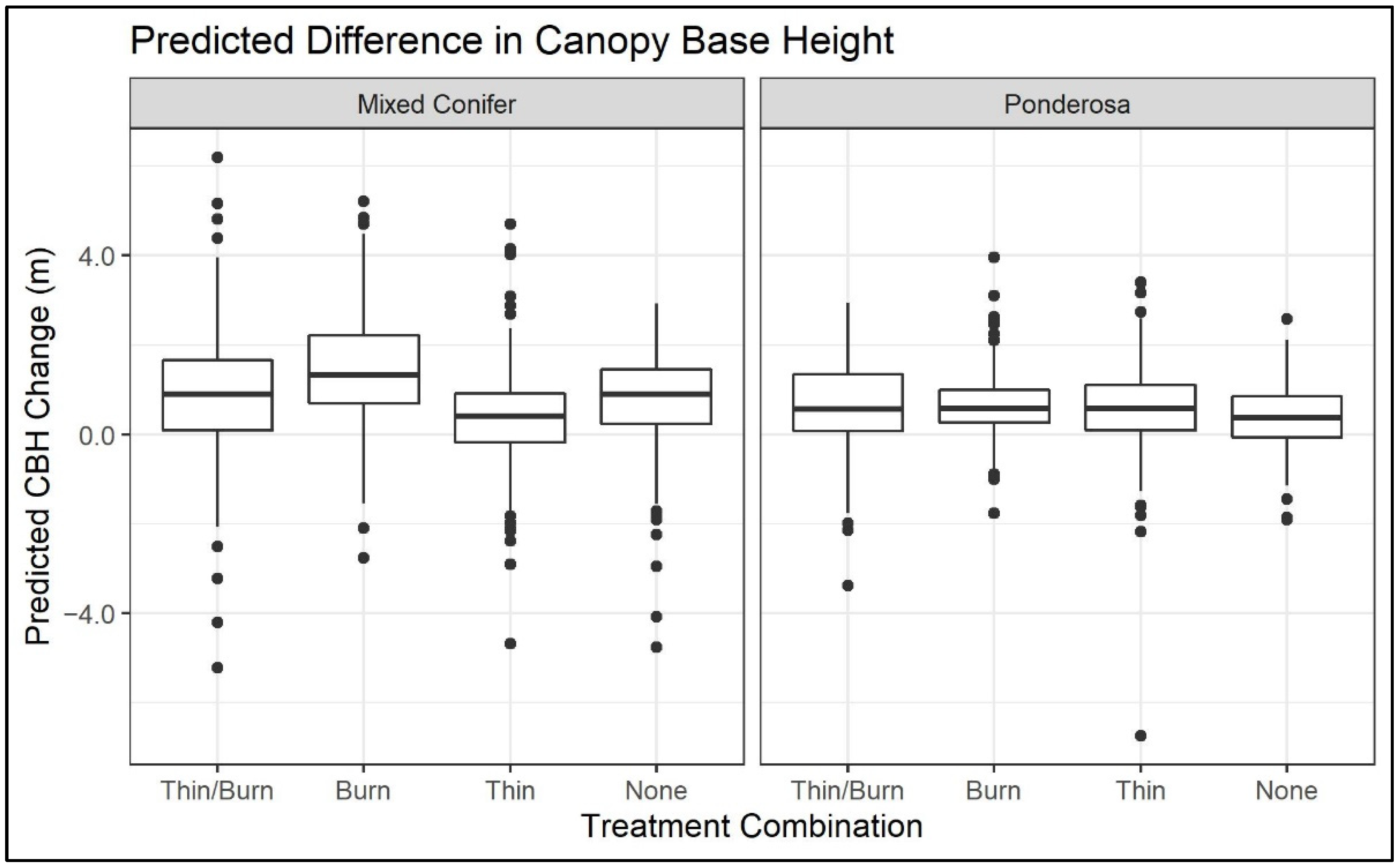
3.1. Canopy Base Height (CBH)
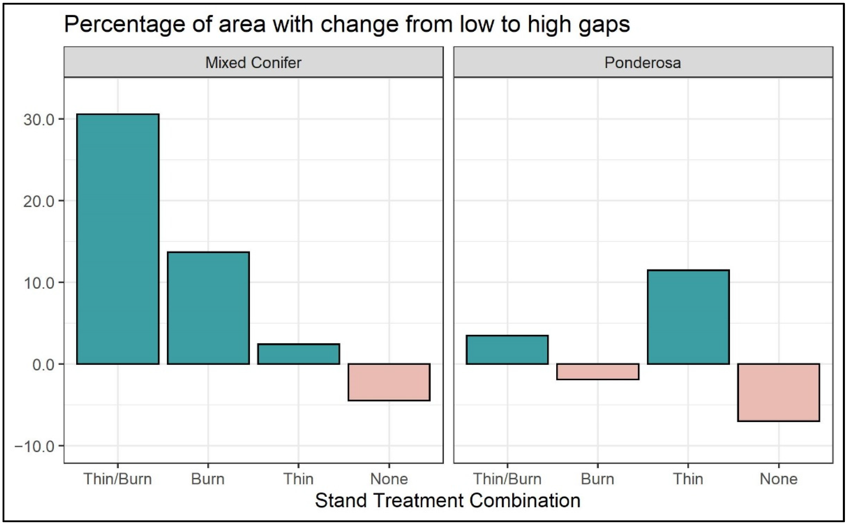
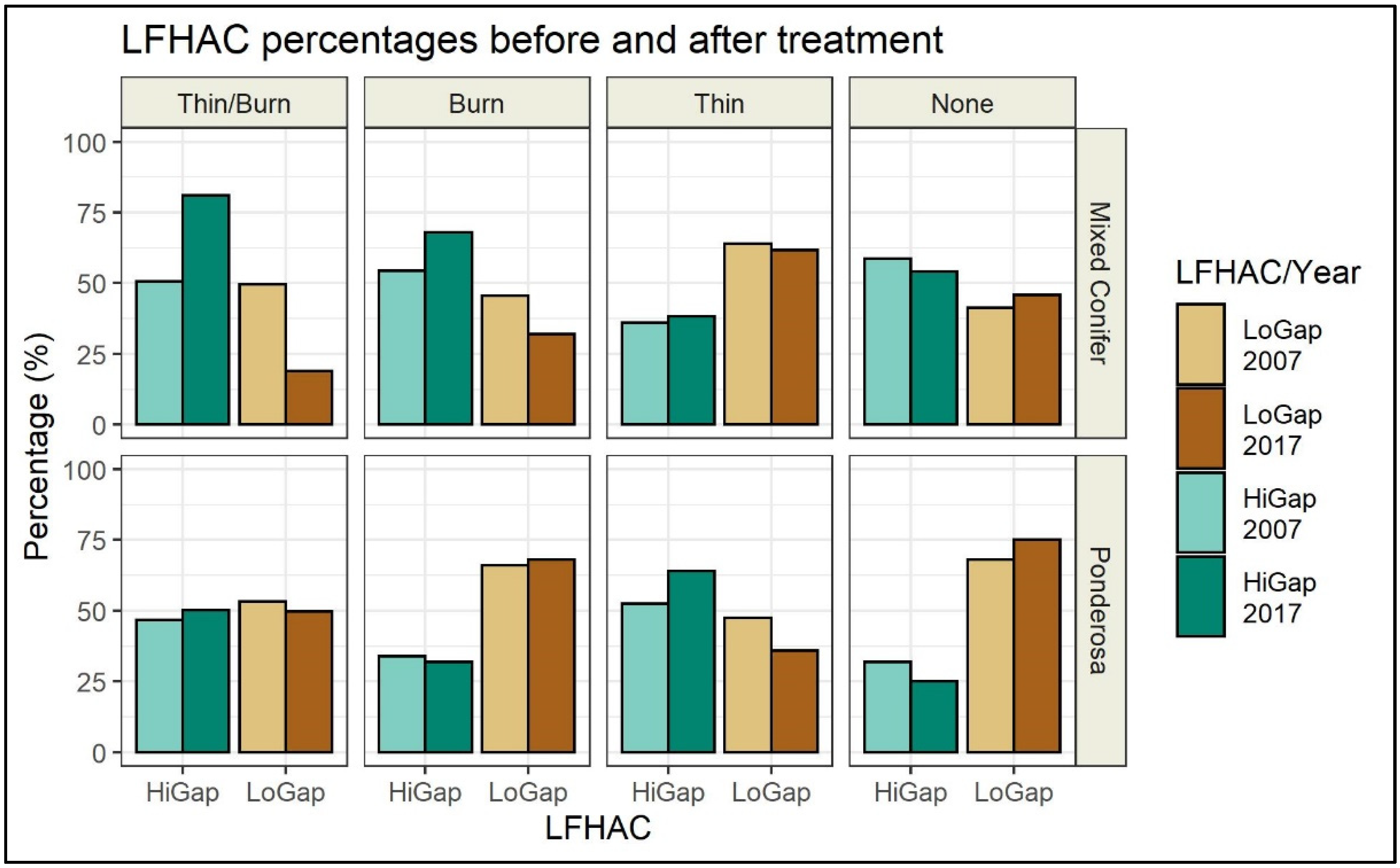
3.2. Ladder Fuel Hazard Assessment Class (LFHAC)
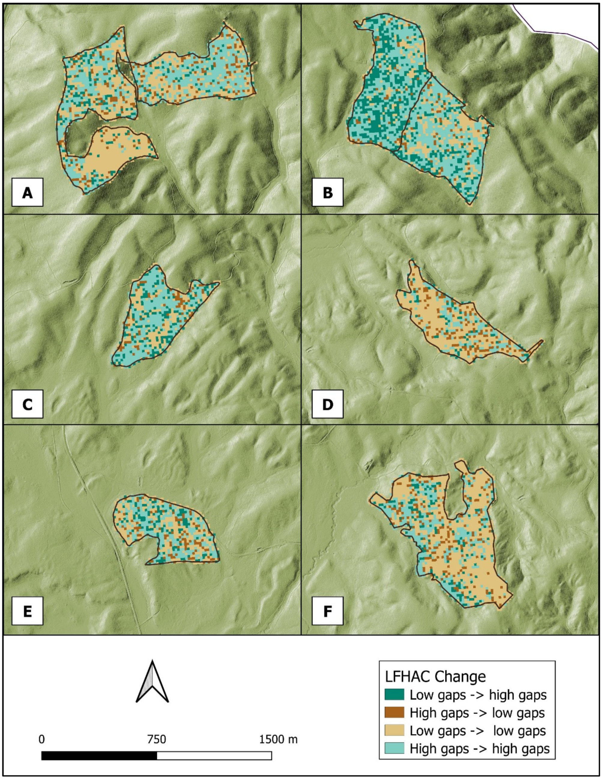
4. Discussion
5. Conclusions
Author Contributions
Funding
Data Availability Statement
Acknowledgments
Conflicts of Interest
Appendix A

| LiDAR Metric | Description |
|---|---|
| Elev_max | Maximum return elevation |
| Elev_mean | Mean return elevation |
| Elev_mode | Mode return elevation |
| Elev_stddev | Standard deviation return elevations |
| Elev_variance | Variance of return elevations |
| Elev_CV | Coefficient of variation of return elevations |
| Elev_skewness | Skewness of return elevations |
| Elev_kurtosis | Kurtosis of return elevations |
| Elev_P01 | 1st percentile return elevation |
| Elev_P10 | 5th percentile return elevation |
| Elev_P20 | 10th percentile return elevation |
| Elev_P25 | 20th percentile return elevation |
| Elev_P30 | 25th percentile return elevation |
| Elev_P40 | 30th percentile return elevation |
| Elev_P50 | 40th percentile return elevation |
| Elev_P60 | 50th percentile return elevation |
| Elev_P70 | 60th percentile return elevation |
| Elev_P75 | 70th percentile return elevation |
| Elev_P80 | 75th percentile return elevation |
| Elev_P90 | 80th percentile return elevation |
| Elev_P95 | 90th percentile return elevation |
| Elev_P99 | 95th percentile return elevation |
| Elev_P60 | 99th percentile return elevation |
| Elev_P70 | Proportion of returns below 2 m |
| Elev_P75 | Proportion of returns between 2 m and 4 m |
| Elev_P80 | Proportion of returns between 4 m and 6 m |
| Elev_P90 | Proportion of returns between 6 m and 8 m |
| Elev_P95 | Proportion of returns below 4 m |
| Elev_P99 | Proportion of returns below 6 m |
| Elev_P60 | Proportion of returns below 8 m |
| Elev_P70 | Proportion of returns between 2 m and 6 m |
| Elev_P75 | Proportion of returns between 2 m and 8 m |
References
- Miller, C. The hidden consequences of fire suppression. Park Sci. 2011, 28, 75–80. [Google Scholar]
- van Wagtendonk, J.W. The History and Evolution of Wildland Fire Use. Fire Ecol. 2007, 3, 3–17. [Google Scholar] [CrossRef]
- Hanberry, B.B. Compositional changes in selected forest ecosystems of the western United States. Appl. Geogr. 2014, 52, 90–98. [Google Scholar] [CrossRef]
- Hessburg, P.F.; Agee, J.K.; Franklin, J.F. Dry forests and wildland fires of the inland Northwest USA: Contrasting the landscape ecology of the pre-settlement and modern eras. For. Ecol. Manag. 2005, 211, 117–139. [Google Scholar] [CrossRef]
- Higuera, P.E.; Metcalf, A.L.; Miller, C.; Buma, B.; McWethy, D.B.; Metcalf, E.C.; Ratajczak, Z.; Nelson, C.R.; Chaffin, B.C.; Stedman, R.C.; et al. Integrating Subjective and Objective Dimensions of Resilience in Fire-Prone Landscapes. BioScience 2019, 69, 379–388. [Google Scholar] [CrossRef] [Green Version]
- Johnstone, J.F.; Allen, C.D.; Franklin, J.F.; Frelich, L.E.; Harvey, B.J.; Higuera, P.E.; Mack, M.C.; Meentemeyer, R.K.; Metz, M.R.; Perry, G.L.W.; et al. Changing disturbance regimes, ecological memory, and forest resilience. Front. Ecol. Environ. 2016, 14, 369–378. [Google Scholar] [CrossRef]
- Stevens-Rumann, C.S.; Kemp, K.B.; Higuera, P.E.; Harvey, B.J.; Rother, M.T.; Donato, D.C.; Morgan, P.; Veblen, T.T. Evidence for declining forest resilience to wildfires under climate change. Ecol. Lett. 2018, 21, 243–252. [Google Scholar] [CrossRef]
- Fiedler, C.E.; Arno, S.F.; Harrington, M.G. Reintroducing fire in ponderosa pine-fir forests after a century of fire exclusion. In Fire in Ecosystem Management: Shifting the Paradigm from Suppression to Prescription. Tall Timbers Fire Ecology Conference Proceedings; Tall Timbers Research Station: Tallahassee, FL, USA, 1998; pp. 245–249. [Google Scholar]
- Lydersen, J.M.; Collins, B.M.; Knapp, E.E.; Roller, G.B. Relating fuel loads to overstorey structure and composition in a fire-excluded Sierra Nevada mixed conifer forest. Int. J. Wildland Fire 2015, 24, 484–494. [Google Scholar] [CrossRef]
- Finney, M.A.; Seli, R.C.; McHugh, C.W.; Ager, A.A.; Bahro, B.; Agee, J.K. Simulation of long-term landscape-level fuel treatment effects on large wildfires. Int. J. Wildland Fire 2007, 16, 712–727. [Google Scholar] [CrossRef] [Green Version]
- Keane, R.E. Describing wildland surface fuel loading for fire management: A review of approaches, methods, and systems. Int. J. Wildland Fire 2013, 22, 51–62. [Google Scholar] [CrossRef]
- Agee, J.K.; Skinner, C.N. Basic principles of forest fuel reduction treatments. For. Ecol. Manag. 2005, 211, 83–96. [Google Scholar] [CrossRef]
- Hessburg, P.F.; Churchill, D.J.; Larson, A.J.; Haugo, R.D.; Miller, C.; Spies, T.A.; North, M.P.; Povak, N.A.; Belote, R.T.; Singleton, P.H.; et al. Restoring fire-prone Inland Pacific landscapes: Seven core principles. Landsc. Ecol. 2015, 30, 1805–1835. [Google Scholar] [CrossRef] [Green Version]
- Brown, R.T.; Agee, J.K.; Franklin, J.F. Forest restoration and fire: Principles in the context of place. Conserv. Biol. 2004, 18, 903–912. [Google Scholar] [CrossRef]
- Stephens, S.L.; Collins, B.M.; Biber, E.; Fulé, P.Z. U.S. federal fire and forest policy: Emphasizing resilience in dry forests. Ecosphere 2016, 7, e01584. [Google Scholar] [CrossRef]
- Bailey, J.D.; Covington, W.W. Evaluating ponderosa pine regeneration rates following ecological restoration treatments in northern Arizona, USA. For. Ecol. Manag. 2002, 155, 271–278. [Google Scholar] [CrossRef]
- Fulé, P.Z.; Crouse, J.E.; Roccaforte, J.P.; Kalies, E.L. Do thinning and/or burning treatments in western USA ponderosa or Jeffrey pine-dominated forests help restore natural fire behavior? For. Ecol. Manag. 2012, 269, 68–81. [Google Scholar] [CrossRef]
- Stanturf, J.A.; Palik, B.J.; Dumroese, R.K. Contemporary forest restoration: A review emphasizing function. For. Ecol. Manag. 2014, 331, 292–323. [Google Scholar] [CrossRef]
- Franklin, J.F.; Johnson, K.N. A Restoration Framework for Federal Forests in the Pacific Northwest. J. For. 2012, 110, 429–439. [Google Scholar] [CrossRef] [Green Version]
- Kalies, E.L.; Yocom Kent, L.L. Tamm Review: Are fuel treatments effective at achieving ecological and social objectives? A systematic review. For. Ecol. Manag. 2016, 375, 84–95. [Google Scholar] [CrossRef] [Green Version]
- Haugo, R.; Zanger, C.; DeMeo, T.; Ringo, C.; Shlisky, A.; Blankenship, K.; Simpson, M.; Mellen-McLean, K.; Kertis, J.; Stern, M. A new approach to evaluate forest structure restoration needs across Oregon and Washington, USA. For. Ecol. Manag. 2015, 335, 37–50. [Google Scholar] [CrossRef] [Green Version]
- Urgenson, L.S.; Ryan, C.M.; Halpern, C.B.; Bakker, J.D.; Belote, R.T.; Franklin, J.F.; Haugo, R.D.; Nelson, C.R.; Waltz, A.E.M. Visions of Restoration in Fire-Adapted Forest Landscapes: Lessons from the Collaborative Forest Landscape Restoration Program. Environ. Manag. 2017, 59, 338–353. [Google Scholar] [CrossRef]
- United States Congress. Omnibus Public Land Management Act of 2009; Pub. L. No. 111-11, Title IV; United States Congress: Washington, DC, USA, 2009.
- USDA Forest Service Washington Office CFLRP Staff. Collaborative Forest Landscape Restoration Program: Ten Years of Results and Lessons Learned: A Comprehensive Review of Results and Lessons Learned from Ten Years of CFLRP Implementation. 2020. Available online: https://www.fs.fed.us/restoration/documents/cflrp/CFLRP_LessonsLearnedCompiled20201016.pdf (accessed on 7 February 2022).
- Schultz, C.A.; Coelho, D.L.; Beam, R.D. Design and governance of multiparty monitoring under the USDA Forest Service’s Collaborative Forest Landscape Restoration Program. J. For. 2014, 112, 198–206. [Google Scholar] [CrossRef]
- Wurtzebach, Z.; Schultz, C.; Waltz, A.E.M.; Esch, B.E.; Wasserman, T.N. Broader-Scale Monitoring for Federal Forest Planning: Challenges and Opportunities. J. For. 2019, 117, 244–255. [Google Scholar] [CrossRef]
- Esch, B.E.; Waltz, A.E.M. Assessing metrics of landscape restoration success in Collaborative Forest Landscape Restoration Projects. In ERI White Paper—Issues in Forest Restoration; Ecological Restoration Institute, Northern Arizona University: Flagstaff, AZ, USA, 2019. [Google Scholar]
- Andersen, H.E.; McGaughey, R.J.; Reutebuch, S.E. Estimating forest canopy fuel parameters using LIDAR data. Remote Sens. Environ. 2005, 94, 441–449. [Google Scholar] [CrossRef]
- Reutebuch, S.E.; Andersen, H.-E.; McGaughey, R.J. Light Detection and Ranging (LIDAR): An Emerging Tool for Multiple Resource Inventory. J. For. 2005, 103, 286–292. [Google Scholar] [CrossRef]
- Hall, S.A.; Burke, I.C.; Box, D.O.; Kaufmann, M.R.; Stoker, J.M. Estimating stand structure using discrete-return lidar: An example from low density, fire prone ponderosa pine forests. For. Ecol. Manag. 2005, 208, 189–209. [Google Scholar] [CrossRef]
- Richardson, J.J.; Moskal, L.M. Strengths and limitations of assessing forest density and spatial configuration with aerial LiDAR. Remote Sens. Environ. 2011, 115, 2640–2651. [Google Scholar] [CrossRef]
- Hoe, M.S.; Dunn, C.J.; Temesgen, H. Multitemporal LiDAR improves estimates of fire severity in forested landscapes. Int. J. Wildland Fire 2018, 27, 581. [Google Scholar] [CrossRef]
- McCarley, T.R.; Kolden, C.A.; Vaillant, N.M.; Hudak, A.T.; Smith, A.M.S.; Wing, B.M.; Kellogg, B.S.; Kreitler, J. Multi-temporal LiDAR and Landsat quantification of fire-induced changes to forest structure. Remote Sens. Environ. 2017, 191, 419–432. [Google Scholar] [CrossRef] [Green Version]
- Duncanson, L.; Dubayah, R. Monitoring individual tree-based change with airborne lidar. Ecol. Evol. 2018, 8, 5079–5089. [Google Scholar] [CrossRef]
- Marinelli, D.; Paris, C.; Bruzzone, L. A Novel Approach to 3-D Change Detection in Multitemporal LiDAR Data Acquired in Forest Areas. IEEE Trans. Geosci. Remote Sens. 2018, 56, 3030–3046. [Google Scholar] [CrossRef]
- Wasserman, T.N.; Sánchez Meador, A.J.; Waltz, A.E.M. Grain and Extent Considerations Are Integral for Monitoring Landscape-Scale Desired Conditions in Fire-Adapted Forests. Forests 2019, 10, 465. [Google Scholar] [CrossRef] [Green Version]
- Edson, C.; Wing, M.G. Airborne Light Detection and Ranging (LiDAR) for Individual Tree Stem Location, Height, and Biomass Measurements. Remote Sens. 2011, 3, 2494–2528. [Google Scholar] [CrossRef] [Green Version]
- Hudak, A.T.; Evans, J.S.; Smith, A.M.S. LiDAR utility for natural resource managers. Remote Sens. 2009, 1, 934–951. [Google Scholar] [CrossRef] [Green Version]
- Sheridan, R.D.; Popescu, S.C.; Gatziolis, D.; Morgan, C.L.S.; Ku, N.W. Modeling forest aboveground biomass and volume using airborne LiDAR metrics and forest inventory and analysis data in the Pacific Northwest. Remote Sens. 2015, 7, 229–255. [Google Scholar] [CrossRef]
- Jakubowksi, M.K.; Guo, Q.; Collins, B.; Stephens, S.; Kelly, M. Predicting Surface Fuel Models and Fuel Metrics Using Lidar and CIR Imagery in a Dense, Mountainous Forest. Photogramm. Eng. Remote Sens. 2013, 79, 37–49. [Google Scholar] [CrossRef] [Green Version]
- Tappeiner, J.C.; Maguire, D.A.; Harrington, T.B.; Bailey, J.D. Chapter 11: Fire and Silviculture. In Silviculture and Ecology of Western U.S. Forests; Oregon State University Press: Corvallis, OR, USA, 2015; pp. 316–348. [Google Scholar]
- Chamberlain, C.P.; Sánchez Meador, A.J.; Thode, A.E. Airborne lidar provides reliable estimates of canopy base height and canopy bulk density in southwestern ponderosa pine forests. For. Ecol. Manag. 2021, 481, 118695. [Google Scholar] [CrossRef]
- Menning, K.M.; Stephens, S.L. Fire Climbing in the Forest: A Semiqualitative, Semiquantitative Approach to Assessing Ladder Fuel Hazards. West. J. Appl. For. 2007, 22, 88–93. [Google Scholar] [CrossRef] [Green Version]
- Kramer, H.; Collins, B.; Kelly, M.; Stephens, S. Quantifying Ladder Fuels: A New Approach Using LiDAR. Forests 2014, 5, 1432–1453. [Google Scholar] [CrossRef]
- Malheur National Forest. Damon Wildland Urban Interface Project—Environmental Assessment. 2010. Available online: https://www.fs.usda.gov/nfs/11558/www/nepa/47110_FSPLT1_025758.pdf (accessed on 7 February 2022).
- Johnston, J.D.; Bailey, J.D.; Dunn, C.J. Influence of fire disturbance and biophysical heterogeneity on pre-settlement ponderosa pine and mixed conifer forests. Ecosphere 2016, 7, e01581. [Google Scholar] [CrossRef]
- ESRI. ArcMap. (Version 10.6) [Software]. 2018. Available online: http://desktop.arcgis.com/en/arcmap/ (accessed on 7 February 2022).
- Trimble. Trimble GPS Pathfinder Office. Trimble Geospatial. 2018. Available online: https://geospatial.trimble.com/products-and-solutions/gps-pathfinder-office (accessed on 7 February 2022).
- PRWeb. Quantum Spatial Formed though Merger of AeroMetric, Photo Science and WSI. 2013. Available online: https://www.prweb.com/releases/2013/9/prweb11086471.htm (accessed on 6 January 2019).
- Rapidlasso. LAStools. [Software]. 2018. Available online: https://rapidlasso.com/LAStools/ (accessed on 7 February 2022).
- NOAA. VDatum. (Version 3.9). [Software]. 2018. Available online: https://www.vdatum.noaa.gov/ (accessed on 7 February 2022).
- Hijmans, R. Geosphere. (R Package Version 1.5-7). [Software]. 2017. Available online: https://cran.r-project.org/web/packages/geosphere/index.html (accessed on 7 February 2022).
- McGaughey, R. FUSION. (Version 3.80). [Software]. 2018. Available online: http://forsys.cfr.washington.edu/fusion/fusionlatest.html (accessed on 7 February 2022).
- Lumley, T.; Miller, A. Leaps: Regression Subset Selection. R Package Version 3.0. [Software]. 2017. Available online: https://cran.r-project.org/web/packages/leaps/index.html (accessed on 7 February 2022).
- Breiman, L. Random forests. Mach. Learn. 2001, 45, 29. [Google Scholar] [CrossRef] [Green Version]
- Liaw, A.; Wiener, M. Classification and Regression by randomForest. R News 2002, 2, 18–22. Available online: https://cran.r-project.org/doc/Rnews/ (accessed on 7 February 2022).
- Breiman, L.; Cutler, A. (n.d.) Random Forests: Balancing Prediction Error. [Web]. Available online: https://www.stat.berkeley.edu/~breiman/RandomForests/cc_home.htm (accessed on 7 February 2022).
- Kane, V.R.; North, M.P.; Lutz, J.A.; Churchill, D.J.; Roberts, S.L.; Smith, D.F.; McGaughey, R.J.; Kane, J.T.; Brooks, M.L. Assessing fire effects on forest spatial structure using a fusion of Landsat and airborne LiDAR data in Yosemite National Park. Remote Sens. Environ. 2014, 151, 89–101. [Google Scholar] [CrossRef]
- Youngblood, A.; Wright, C.S.; Ottmar, R.D.; McIver, J.D. Changes in fuelbed characteristics and resulting fire potentials after fuel reduction treatments in dry forests of the Blue Mountains, northeastern Oregon. For. Ecol. Manag. 2008, 255, 3151–3169. [Google Scholar] [CrossRef]
- Clark, E.; (Malheur National Forest, USDA Forest Service). Personal Communication, 17 October 2019.
- Erdody, T.L.; Moskal, L.M. Fusion of LiDAR and imagery for estimating forest canopy fuels. Remote Sens. Environ. 2010, 114, 725–737. [Google Scholar] [CrossRef]
- Stefanidou, A.; Gitas, I.Z.; Korhonen, L.; Stavrakoudis, D.; Georgopoulos, N. LiDAR-Based Estimates of Canopy Base Height for a Dense Uneven-Aged Structured Forest. Remote Sens. 2020, 12, 1565. [Google Scholar] [CrossRef]
- Stephens, S.L.; Collins, B.M.; Roller, G. Fuel treatment longevity in a Sierra Nevada mixed conifer forest. For. Ecol. Manag. 2012, 285, 204–212. [Google Scholar] [CrossRef]
- Vaillant, N.M.; Noonan-Wright, E.K.; Reiner, A.L.; Ewell, C.M.; Rau, B.M.; Fites-Kaufman, J.A.; Dailey, S.N. Fuel accumulation and forest structure change following hazardous fuel reduction treatments throughout California. Int. J. Wildland Fire 2015, 24, 361–371. [Google Scholar] [CrossRef]
- Hummel, S.; Hudak, A.T.; Uebler, E.H.; Falkowski, M.J.; Megown, K.A. A comparison of accuracy and cost of LiDAR versus stand exam data for landscape management on the Malheur National Forest. J. For. 2011, 109, 267–273. [Google Scholar] [CrossRef]
- Donager, J.J.; Sankey, T.T.; Sankey, J.B.; Sanchez Meador, A.J.; Springer, A.E.; Bailey, J.D. Examining Forest Structure With Terrestrial Lidar: Suggestions and Novel Techniques Based on Comparisons Between Scanners and Forest Treatments. Earth Space Sci. 2018, 5, 753–776. [Google Scholar] [CrossRef] [Green Version]
- LaRue, E.A.; Wagner, F.W.; Fei, S.; Atkins, J.W.; Fahey, R.T.; Gough, C.M.; Hardiman, B.S. Compatibility of aerial and terrestrial LiDAR for quantifying forest structural diversity. Remote Sens. 2020, 12, 1407. [Google Scholar] [CrossRef]
- Cunliffe, A.M.; Brazier, R.E.; Anderson, K. Ultra-fine grain landscape-scale quantification of dryland vegetation structure with drone-acquired structure-from-motion photogrammetry. Remote Sens. Environ. 2016, 183, 129–143. [Google Scholar] [CrossRef] [Green Version]
- Iglhaut, J.; Cabo, C.; Puliti, S.; Piermattei, L.; O’Connor, J.; Rosette, J. Structure from Motion Photogrammetry in Forestry: A Review. Curr. For. Rep. 2019, 5, 155–168. [Google Scholar] [CrossRef] [Green Version]
- Charnley, S.; Kelly, E.C.; Fischer, A.P. Fostering collective action to reduce wildfire risk across property boundaries in the American West. Environ. Res. Lett. 2020, 15, 025007. [Google Scholar] [CrossRef]


| Class | Surface Fuels | Gaps |
|---|---|---|
| A | High | <2 m (low) |
| B | High | >2 m (high) |
| C | Low | <2 m (low) |
| D | Low | >2 m (high) |
| E | Non-Forest | Non-Forest |
| Forest Type | Treatment | Avg CBH 2007 (m) | Avg CBH 2017 (m) | Avg Change (m) | Min Change (m) | Max Change (m) |
|---|---|---|---|---|---|---|
| Mixed Conifer | Thin/Burn | 4.42 | 5.31 | 0.89 | −5.21 | 6.20 |
| Mixed Conifer | Burn | 4.54 | 5.97 | 1.43 | −2.77 | 5.21 |
| Mixed Conifer | Thin | 3.18 | 3.55 | 0.36 | −4.68 | 4.71 |
| Mixed Conifer | None | 4.76 | 5.56 | 0.80 | −4.76 | 2.93 |
| Ponderosa | Thin/Burn | 3.56 | 4.18 | 0.62 | −3.39 | 2.95 |
| Ponderosa | Burn | 2.51 | 3.16 | 0.66 | −1.77 | 3.96 |
| Ponderosa | Thin | 3.73 | 4.32 | 0.60 | −6.74 | 3.40 |
| Ponderosa | None | 2.51 | 2.95 | 0.44 | −1.90 | 2.57 |
| Forest Type | Treatment | Area with Lift (%) |
|---|---|---|
| Mixed Conifer | Thin/Burn | 77.1 |
| Mixed Conifer | Burn | 89.1 |
| Mixed Conifer | Thin | 69.4 |
| Mixed Conifer | None | 82.6 |
| Ponderosa | Thin/Burn | 75.9 |
| Ponderosa | Burn | 87.2 |
| Ponderosa | Thin | 78.3 |
| Ponderosa | None | 70.3 |
| Total Observed | Predicted LoGap | Predicted HiGap | Classification Error | |
|---|---|---|---|---|
| LoGap | 62 | 49 | 13 | 0.21 |
| HiGap | 50 | 17 | 33 | 0.34 |
| 2007 | 2017 | Change | ||||
|---|---|---|---|---|---|---|
| Forest Type | Treatment | LoGap (%) | HiGap (%) | LoGap (%) | HiGap (%) | HiGap (%) |
| Mixed Conifer | Thin/Burn | 49.5 | 50.5 | 18.9 | 81.1 | 30.6 |
| Mixed Conifer | Burn | 45.7 | 54.3 | 32.0 | 68.0 | 13.7 |
| Mixed Conifer | Thin | 64.0 | 36.0 | 61.6 | 38.4 | 2.4 |
| Mixed Conifer | None | 41.3 | 58.7 | 45.8 | 54.2 | −4.5 |
| Ponderosa | Thin/Burn | 53.2 | 46.8 | 49.7 | 50.3 | 3.5 |
| Ponderosa | Burn | 66.1 | 33.9 | 68.0 | 32.0 | −1.9 |
| Ponderosa | Thin | 47.5 | 52.5 | 36.0 | 64.0 | 11.5 |
| Ponderosa | None | 68.0 | 32.0 | 75.0 | 25.0 | −7.0 |
Publisher’s Note: MDPI stays neutral with regard to jurisdictional claims in published maps and institutional affiliations. |
© 2022 by the authors. Licensee MDPI, Basel, Switzerland. This article is an open access article distributed under the terms and conditions of the Creative Commons Attribution (CC BY) license (https://creativecommons.org/licenses/by/4.0/).
Share and Cite
Olszewski, J.H.; Bailey, J.D. LiDAR as a Tool for Assessing Change in Vertical Fuel Continuity Following Restoration. Forests 2022, 13, 503. https://doi.org/10.3390/f13040503
Olszewski JH, Bailey JD. LiDAR as a Tool for Assessing Change in Vertical Fuel Continuity Following Restoration. Forests. 2022; 13(4):503. https://doi.org/10.3390/f13040503
Chicago/Turabian StyleOlszewski, Julia H., and John D. Bailey. 2022. "LiDAR as a Tool for Assessing Change in Vertical Fuel Continuity Following Restoration" Forests 13, no. 4: 503. https://doi.org/10.3390/f13040503
APA StyleOlszewski, J. H., & Bailey, J. D. (2022). LiDAR as a Tool for Assessing Change in Vertical Fuel Continuity Following Restoration. Forests, 13(4), 503. https://doi.org/10.3390/f13040503