1. Introduction
In the past decade, there has been a substantial amount of life cycle assessment (LCA) research focused on the commercial production of biofuels from lignocellulosic feedstocks [
1,
2,
3,
4,
5,
6,
7]. Many of these LCAs typically focus only on global impacts (i.e., greenhouse gas emissions and fossil fuel use), as biofuels are intended to help mitigate climate change effects by replacing petroleum-based transportation fuels. Few of the biofuel LCA studies report on regional impacts (i.e., acidification, eutrophication, smog, water use, etc.) [
1,
2,
8,
9], and fewer still take into account the spatial variability of these impacts [
8,
10]. Regional impacts from biofuel feedstock production could prove to be a substantial issue. An LCA study evaluating regional emissions from agricultural systems found that by not including regional emission information, life cycle environmental impacts are likely underestimated [
9]. Another study coupling GIS and LCA found variability in changes to regional biodiversity resulting from the production of ethanol from corn and sugar beets, demonstrating the use and importance of spatially located inventory data in LCAs [
11]. However, effectively accounting for regional impacts cannot be easily addressed when the location of a biorefinery and lands growing the lignocellulosic feedstock is unknown [
10]. This has led to an incomplete view of the life cycle impacts of producing biofuels [
8].
Addressing regionally specific and non-global impacts requires LCAs to incorporate spatial analyses within the scope of research. This approach has yet to become common practice, but research is now starting to be published that unifies biofuel LCAs with geographical information systems (GIS) [
10,
11,
12,
13,
14]. In these studies, the LCAs are used to calculate environmental impacts and GIS are used to spatially locate where the environmental impacts are generated. This allows researchers to identify hot spots and potentially develop solutions to reduce these impacts, such as crop implementation strategies to reduce carbon/energy budgets [
12]. Spatial LCAs can also be used to evaluate potential changes to an area when introducing a new biofuel production system. This is particularly important for systems that involve agricultural practices, where energy crops are grown as feedstock for biofuel production [
13]. Not only is there a lot of spatial variability in agricultural practices [
14], but they also take up large areas of land, making land use change issues a concern. To address these impacts, some researchers, where possible, have used a spatial LCA approach to measure the net effect of environmental impacts that result from switching from one system to another in their respective regions.
Spatially explicit LCAs that are specific to the system and locations that they evaluate have shown that when site-specific factors are considered, there can be substantial variability in LCA results [
10,
12,
13,
14]. Agricultural practices are not static and vary from one region to the next [
8,
9,
14]. For biofuel systems that use (a) feedstock(s) with (a) lower carbon footprint(s), the effect of agricultural variability on total greenhouse gas emissions may be small, but for biofuels based on feedstocks with larger carbon footprints, the overall variability could have a more pronounced effect. Spatially locating biofuel production can therefore help to reduce some of the variability and uncertainty in biofuel LCAs [
10,
12,
13,
14]. Conclusions from these studies further enforce the need to assess biofuel LCAs using spatially explicit LCAs.
In this research, spatial analysis and life cycle methodologies are used to help identify regional land use changes and potential environmental impacts associated with converting lands from rangeland and croplands to growing poplar trees for biofuel production. This work builds on the LCA research presented in Budsberg et al., 2016 [
15], and uses the same biorefinery model that is designed to produce bio-jet fuel from poplar biomass. Cradle-to-biorefinery gate analyses for poplar bioenergy plantations are conducted for four regions in the western United States that could potentially host bio-jet fuel biorefineries. These regions are based around biorefineries simulated to be located in Pilchuck WA, Hayden ID, Jefferson OR, and Clarksburg CA. Within these regions, site suitability models identify lands that could potentially be converted to poplar crop production and feedstock transportation distances. Poplar crop management and site-specific emissions are based on data collected from poplar pilot farms near each of the four proposed biorefinery locations. These results will help complete the picture of potential life cycle environmental impacts, resulting from a commercial scale biofuels industry in the western United States.
2. Materials and Methods
Life cycle assessment methodology is used to assess cradle-to-biorefinery gate environmental impacts for the production of bio-jet fuel at four locations. The functional unit for each region is the annualized feedstock production and harvesting to support each respective biorefinery producing bio-jet fuel from a poplar feedstock. The biorefinery is assumed to produce 380 million liters (100 million gallons) of jet fuel from 1.25 million tons of poplar biomass, annually. Biorefinery design and process operations are described in detail in Crawford et al., 2016 [
16]. To determine the average annual operations, the biorefinery is modeled to operate for 21 years and the data are then annualized. A 21-year time horizon is chosen so as to include the lifespan of a poplar tree farm (site preparation, nursery operations, and six–three-year coppice cycles) [
15]. The study is not a complete LCA, as the work only addresses changes in the life cycle inventories within each region when a biorefinery is introduced into the area and poplar trees are grown to meet feedstock demands. The only characterization factors assessed are the 100-year global warming potential [
17] and fossil fuel use, so as to make comparisons with a previous non-site-specific LCA study that evaluated the same biorefinery design used in this research [
15]. Fossil fuel use (FFU) is calculated by adding up all fossil fuel inputs (coal, natural gas, crude oil) used to convert the poplar into bio-jet fuel [
18]. No sensitivity or statistical analysis was conducted as these assessments were beyond the scope of work for this research. Results are used to make comparisons between regions without assessing for statistically significant differences.
SimaPro v.8.0 is used to manage life cycle inventories. LCI data are combined with crop displacement data from researchers at UC Davis. These results are integrated and reported using regional maps created using ArcGIS v.10 mapping software. Physical boundaries are defined in each region by the lands converted to growing poplar for bio-jet fuel production. The resolution is 8 × 8 km grids and is defined by data parameters set by the crop displacement models. Life cycle analysis methods are used to calculate changes in land management and evaluate the change (net effect) to each grid block. These methods include conducting life cycle inventories of all crops that could be displaced for each region, and then assigning these data to each crop located within a given grid block. Life cycle inventories are also completed for poplar crops for each region. See
Appendix A for the poplar growth and harvesting data for each region. These results are used to identify changes at the 8 × 8 km grid level, and combined to calculate the total impact to each region. Modeling tools and data collection are further described below.
We use a combination of models to simulate how an economically driven industry would organize to identify the locations of poplar plantations and the incumbent land uses displaced by these plantations. The simulation uses modeled yields of hybrid poplar that are spatially resolved to inform an agricultural economic model of land conversion of croplands to poplar plantations based on farm gate poplar prices. The Geospatial Bioenergy System Model (GBSM) is used to evaluate which combination of plantations will result in the lowest cost of fuel production, while improving the economic outcomes for farmers over the current cropping pattern [
19]. The simulation results in a land use change pattern that would enable the continuous operation of a biorefinery that demands 1.25 million tons of poplar biomass per year. These models are described in more detail below.
Poplar crop yields are dependent on local climate, soils, stocking density, and management practices. The yields are estimated using the 3PG-Coppice model [
20] to capture the variations in these conditions across space. A 16 km
2 grid is used with soil parameters from STATSGO and climate represented as a repeated average year using data from 2000–2014 [
20]. The model simulates growth in the crop using monthly timesteps across the 21-year life of the plantation. Areas that are developed, forested, have slopes greater than 15%, or salinity greater than 4 dS/m, are excluded from the analysis. The poplar yields serve as inputs to the cost of production budgets. These production budgets include all the operations needed to produce a crop. The poplar costs of production are taken from Chudy et al. [
21]. The site-specific costs in Chudy et al. [
21] are generalized across the region by finding the average cost of operations on irrigated and non-irrigated plantations separately, and applying those costs to irrigated and non-irrigated potential poplar plantations.
Poplar adoption by landowners is modeled using a combination of a modified agricultural economic model (SWAP-AHB) and GBSM. SWAP-AHB determines the farm gate prices required to induce a switch to poplar plantations. It is based on the SWAP model [
22] and uses a profit-maximizing objective to allocate land and water resources between poplar and incumbent crops. Incumbent crop production functions are derived from the state-specific cost and return studies for each crop. See
Appendix B for a list of data sources used to model each crop in each region. SWAP has been modified to expand the geographic scope and include poplar as a crop option.
GBSM is a profit-maximizing model of the bioenergy system that sites, sizes, and allocates feedstock resources to biorefineries, incorporating costs of feedstock procurement, transportation, biorefinery capital, and operational costs. It finds the most profitable configuration of biorefinery sites and poplar plantations serving the biorefinery’s demand, given a selling price for the biofuel product. Biomass farm gate prices are taken from SWAP-AHB and a separately calculated willingness-to-accept price for poplar on rangelands. See Parker et al. [
23] and Parker [
24] for more detailed information regarding GBSM. Biorefinery operations are based on the Natural Gas Steam Reforming Bio-jet model in Crawford et al. [
16] and Budsberg et al. [
15]. See these two publications for detailed descriptions and discussions regarding biorefinery design, operating parameters, and life cycle impacts. Through this analysis, the optimized biorefinery locations are Pilchuck Washington, Jefferson Oregon, Hayden Idaho, and Clarksburg California. Transportation distances are reported in the results section as one-way, but round-trip distances were used for estimating fuel use for poplar chip delivery, with the trucks assumed to be fully weighted for delivery and empty for return to poplar farms.
Crops that could potentially be displaced are listed in
Table 1, and crop displacement is determined by profitability. For each given 8 × 8 km square, if poplar is identified as being more profitable than the current crops within that square, it is assumed that poplar would replace that crop. Existing land use is taken from the Cropland Data Layer scaled up to 8 × 8 km grid and scaled to be consistent with the USDA Census of Agricultural crop areas by county, as in Hart et al. [
20]. Two general land types, rangelands and croplands, are identified as eligible for conversion to growing poplar. Rangelands are defined as lands on which the indigenous vegetation is predominately grasses, grass-like plants, forbs, and possibly shrubs or dispersed trees (USDA NRCS—rangeland [
25]). Croplands are those in which adopted crops are grown for harvest (i.e., corn, wheat, peas, etc.) (USDA NRCS—cropland [
26]).
To maintain consistency throughout the research, the life cycle analysis of crop displacement uses the same data sources and assumptions as were used in the SWAP-AHB model. Maintaining this consistency is important, as the SWAP-AHB model takes into account the economics surrounding crop management practices. Modeling decisions to replace a crop with poplar trees are based on the economics associated with data assumptions. Changing data sources and assumptions for the LCA work would introduce inconsistencies within the research, as the assumptions for how each crop is managed are directly related to whether or not it would be displaced to grow poplar trees.
LCIs for crops in each region are developed using regional extension office data [
27,
28,
29,
30], and include the amount of fertilizer, pesticides, water, and fuel used annually to produce a given crop on a hectare of land. Fertilizer use is broken down by the amount of nitrogen, phosphorus, and potassium use. Chemical usage is calculated by aggregating all insecticides, herbicides, and pesticides (by weight) used for a given crop. The annual fuel use for each crop is measured by combining annual diesel and gasoline use (by energy content). As noted, the crop management data for each region are largely based on data from an extension office for that region. Information detailing specific inputs for each displaced crop for each region and the data sources used are listed in
Appendix B.
Poplar growth and management data are supported by operational data from GreenWood Resources and are representative of practices performed at the four poplar demonstration farms located in Pilchuck WA, Jefferson OR, Hayden ID, and Clarksburg, CA. Regional differences in practices are observed at each location and noted, but in general, the growth and harvesting of poplar for bioenergy follow a similar management scheme. Poplar management practices are described in more detail in Budserg et al. [
15] and Budsberg et al. [
18]. See those publications for further discussion regarding poplar crop management. Feedstock production and harvesting life modeling are supported by operational data from industry (Greenwood resources, personal communication 2011–2015), the literature [
31], and LCA databases [
32,
33]. See
Appendix A for a complete list of inputs and management practices used within each region.
N
2O emissions from fertilizer and decaying biomass are calculated using two approaches. The Farm Energy Analysis Tool (FEAT) [
34] is used for general estimates of all four regions. FEAT data are based on multiple poplar and willow growth management publications and provide non-region-specific information regarding greenhouse gas emissions, as well as other input and outputs. Below-ground carbon stores, comprised of above-ground stump (the part that remains after a harvest), below-ground stump, and coarse roots, are included within the system boundaries.
Direct land use change (DLUC) associated with establishing the plantation on land that was previously pasture land is calculated using the Forest Industry Carbon Assessment Tool v.1.3.1.1 [
35]. Tier 1 data [
35] are used to estimate the amount of carbon on these lands that would be released as CO
2 as a result of land use change. More accurate data are not available, as the grid resolution is 64 km
2, and it is unknown exactly how much biomass there is on a given plot of land. IPCC values are used to approximate the relative impact of direct land use change on life cycle carbon emissions. Croplands converted to growing poplar are assumed to have a negligible amount of direct land use change, as these are crops that are turned over annually, and therefore any GHG emissions related to cropland for poplar cultivation would have occurred nevertheless, as a result of the crop management scheme. DLUC is assumed to be a one-time emission when the land is converted from its current state to growing poplar, and is reported separately from the other data. All other aspects of either current land management practices or poplar growth and harvesting are assumed to occur on an ongoing basis, and from this, an ‘average’ year of inputs and outputs can be calculated. This cannot be done with a one-time emission such as DLUC. DLUC is therefore reported separately and addressed by calculating a regional carbon debt payoff. The carbon debt payoff is the time that it will take before the global warming potential savings from switching from current land use practices to poplar production can cancel out the global warming potential emissions generated from DLUC (assuming there are global warming potential savings from switching land use). Indirect land use change is not included in this analysis.
3. Results
The SWAP-AHB and GBSM models projected the types of lands and crops that could switch to growing poplar at a selling price of USD 60 per ton of poplar biomass. Results are presented in
Table 2,
Table 3,
Table 4 and
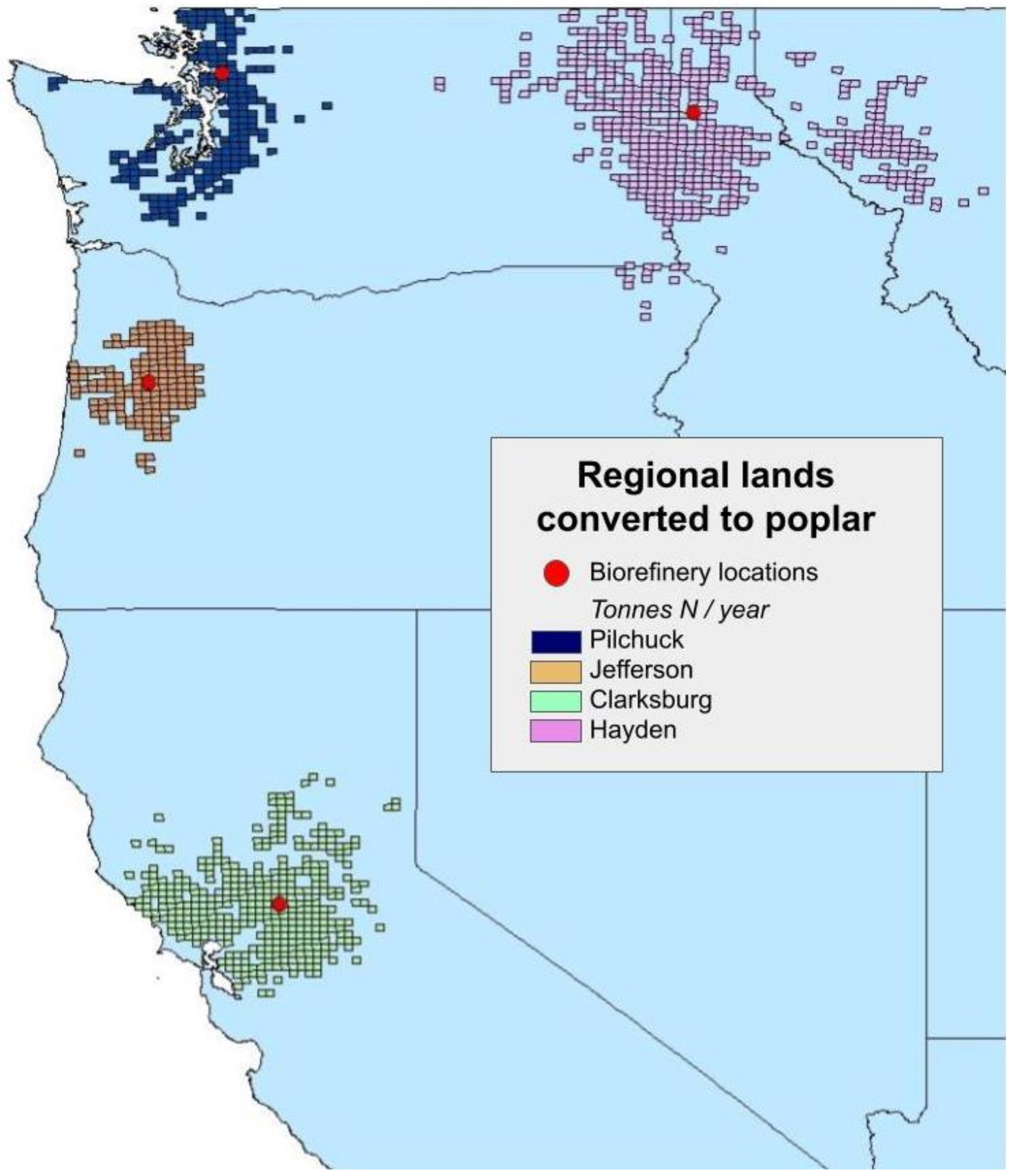
Table 5. The Clarksburg region required the least amount of land to produce 1.25 million BDT of poplar chips per year, followed by Pilchuck, Jefferson, and Hayden, respectively. Compared to Clarksburg, Pilchuck required 30% more land, Jefferson 54% more land, and Hayden 137% more land. The large range in land is due to the projected poplar yields for each region, with Clarksburg expected to have the highest biomass yields, and Hayden the lowest. See
Figure 1 for a spatial overview of lands converted to growing poplar in each region.
Regions also differed in the amount of pasture and cropland converted to growing poplar trees (
Table 2,
Table 3,
Table 4 and
Table 5). The Jefferson region had the most amount of rangeland converted to growing poplar followed by Hayden, Pilchuck, and Clarksburg. On a percentage basis of land converted for each region, almost all of the land in the Jefferson region projected to grow poplar trees would come from rangeland (93%). In the Pilchuck, Hayden, and Clarksburg regions, rangeland is projected to make up 73%, 59%, and 35%, respectively, of the land used to grow poplar. Where croplands are converted to growing poplar, the type of crop converted to poplar differs for each region. In Jefferson, the small amount of cropland converted to poplar is from non-irrigated tame hay (6%) and oats (1%). For the Pilchuck region, the top crops converted include irrigated silage corn (4%) and winter wheat (4%), non-irrigated tame hay (6%), and silage corn (5%). The main crops in the Hayden region are projected to come from irrigated beans (14%), non-irrigated winter wheat (9%), and tame hay (5%). In Clarksburg, the top crops converted are irrigated silage corn (24%), winter wheat (20%), and grain corn (9%). For a list of all crops converted for each region see
Table 2,
Table 3,
Table 4 and
Table 5.
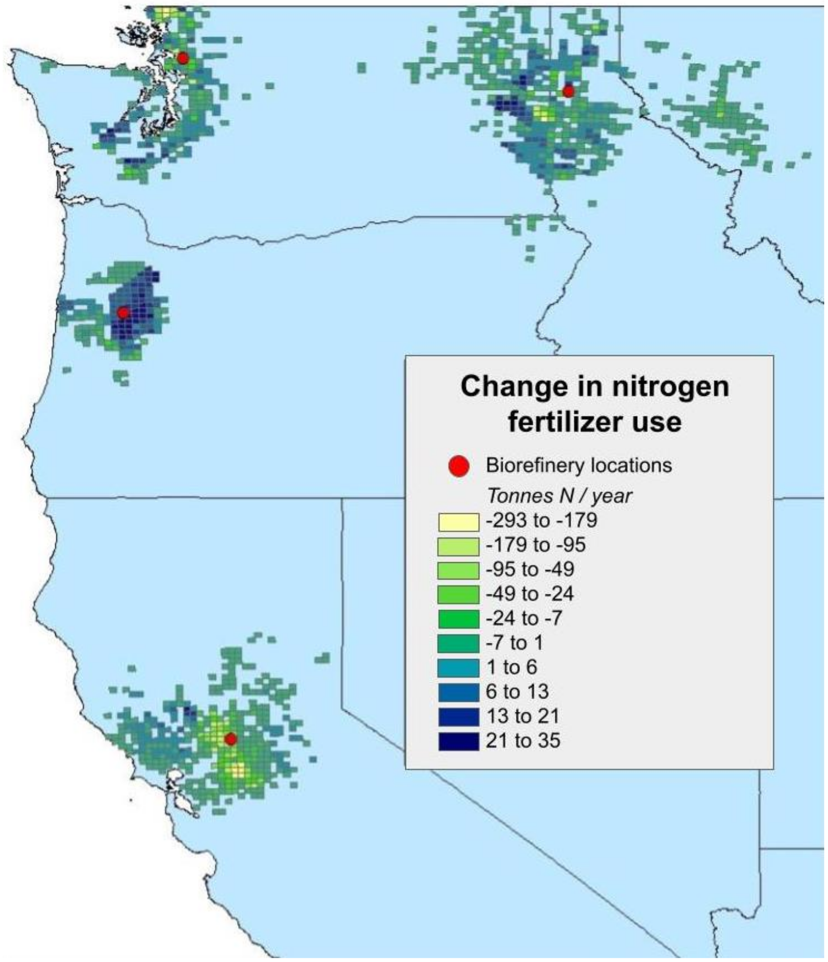
Nitrogen fertilizer was used in all four regions and is also expected to be used when growing poplar trees (
Table 6). Under current active management practices, the Clarksburg region has the highest N fertilizer use, followed by Hayden, Pilchuck, and lastly, Jefferson. Under poplar management schemes, N fertilizer use is projected to be highest in the Hayden region, followed by Jefferson, Pilchuck, and Clarksburg. When lands are converted from their current management state to poplar production, N fertilizer use decreases in three of the four regions: Clarksburg, Pilchuck, and Hayden regions are projected to see N fertilizer use decrease by 82%, 45%, and 17%, respectively. The average rate of application of N fertilizer on actively managed lands will also decrease in these three regions (
Table 6). In the Jefferson region, the N fertilizer average rate of application per hectare of actively managed land will decrease as well, however the total effect on the region will be an N fertilizer use increase of 239%. The rate of N fertilizer application rate for poplar is less than the rate of N fertilizer for tame hay and oats in the Jefferson OR region, but by encouraging poplar growth, a large amount of rangeland (effectively unmanaged with no N fertilizer use) will become actively managed, thereby increasing the total amount of N fertilizer use in the Jefferson region (
Table 6). See
Figure 2 for a spatial visualization of the change in N fertilizer use.
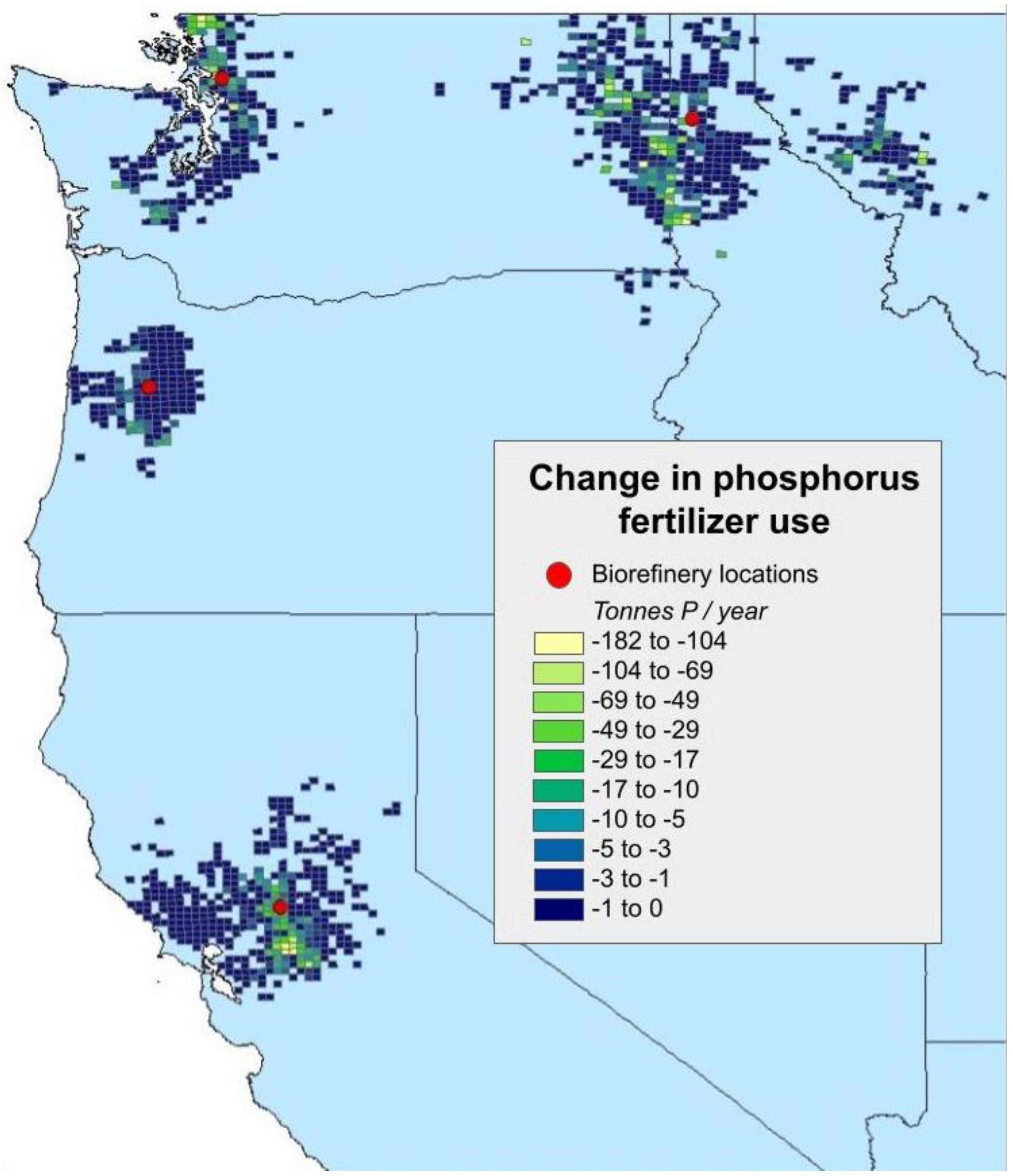
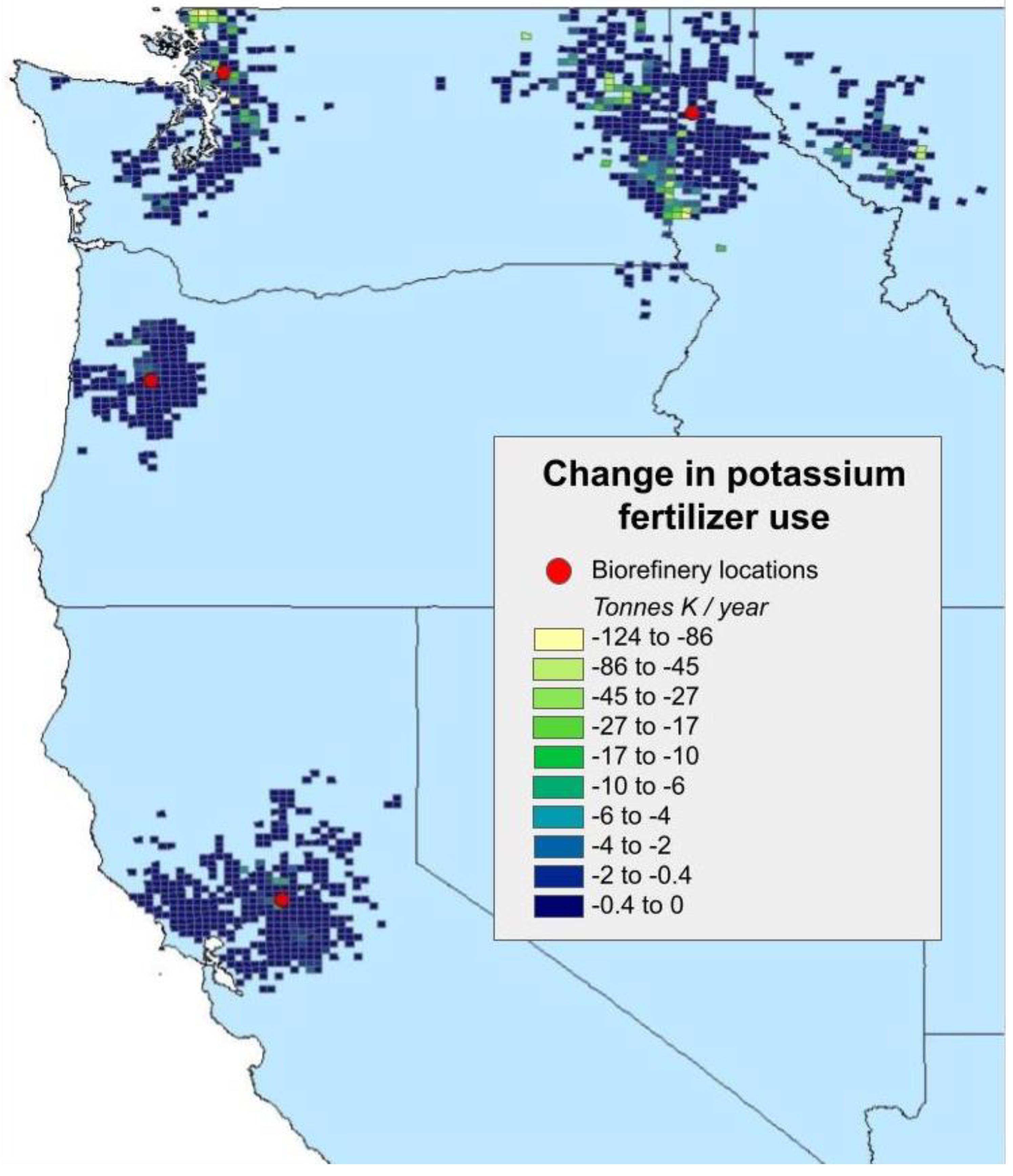
Phosphorus and potassium fertilizers are also currently used in all four regions for growing crops, although not as predominantly as N fertilizer, as not all crops require their inputs. Neither phosphorus nor potassium is projected to be used when growing poplar, therefore switching to a poplar crop results in a 100% decrease of phosphorus and potassium fertilizers in all four regions (
Table 6). On an average rate of application per hectare, the croplands in the Pilchuck region will see the biggest effect of ceasing the use phosphorus (on average, 50 kg P per hectare of cropland per year) and potassium (on average, 41 kg K per hectare of cropland per year). As an entire region, Hayden will see the biggest total effect, where phosphorus and potassium use will go from 2569 tons per year and 1235 tons per year, respectively, to zero. See
Figure 3 and
Figure 4 for a spatial visualization of the change in P and K fertilizer use.
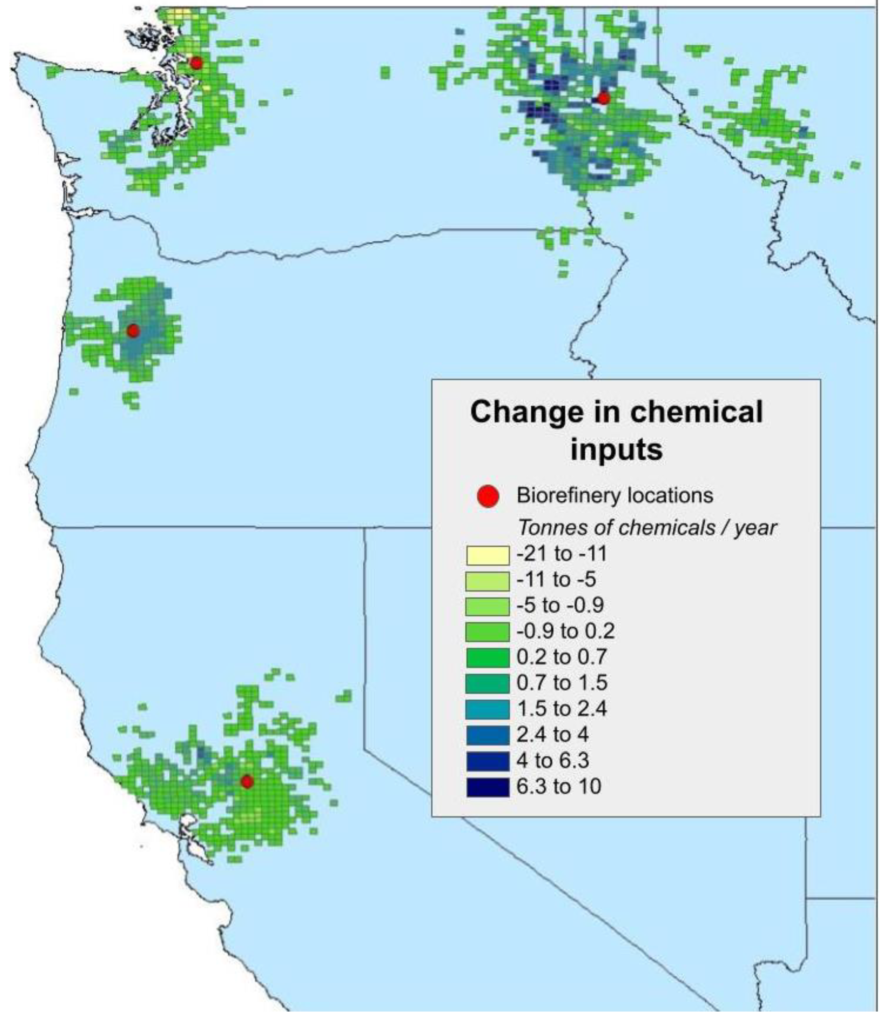
Chemical usage, defined in this study as the use of pesticides, insecticides, and herbicides, occurs in all four regions for the management of current crops, as well as in the growth management of poplar trees (
Table 7). For current actively managed croplands, the total regional use of chemical controls is highest for Hayden, followed by Pilchuck, Clarksburg, and Jefferson. On an average per acre of cropland basis, Hayden has the highest rate of chemical usage, followed by Clarksburg, Jefferson, and Pilchuck. When lands are converted to growing poplar, the average rate of chemical usage remains the lowest in the Pilchuck region. Clarksburg and Jefferson also see a decrease in the average rate of chemical usage, while Hayden is projected to have an increase in the average rate of chemical inputs per hectare when converted to growing poplar. From a total annual regional standpoint, Pilchuck is the only area that is expected to see an overall decrease in chemical inputs. Clarksburg, Hayden, and Jefferson will see regional increases of 18%, 228%, and 511%, respectively (
Table 7). See
Figure 5 for a spatial visualization of the change in chemical pest control inputs.
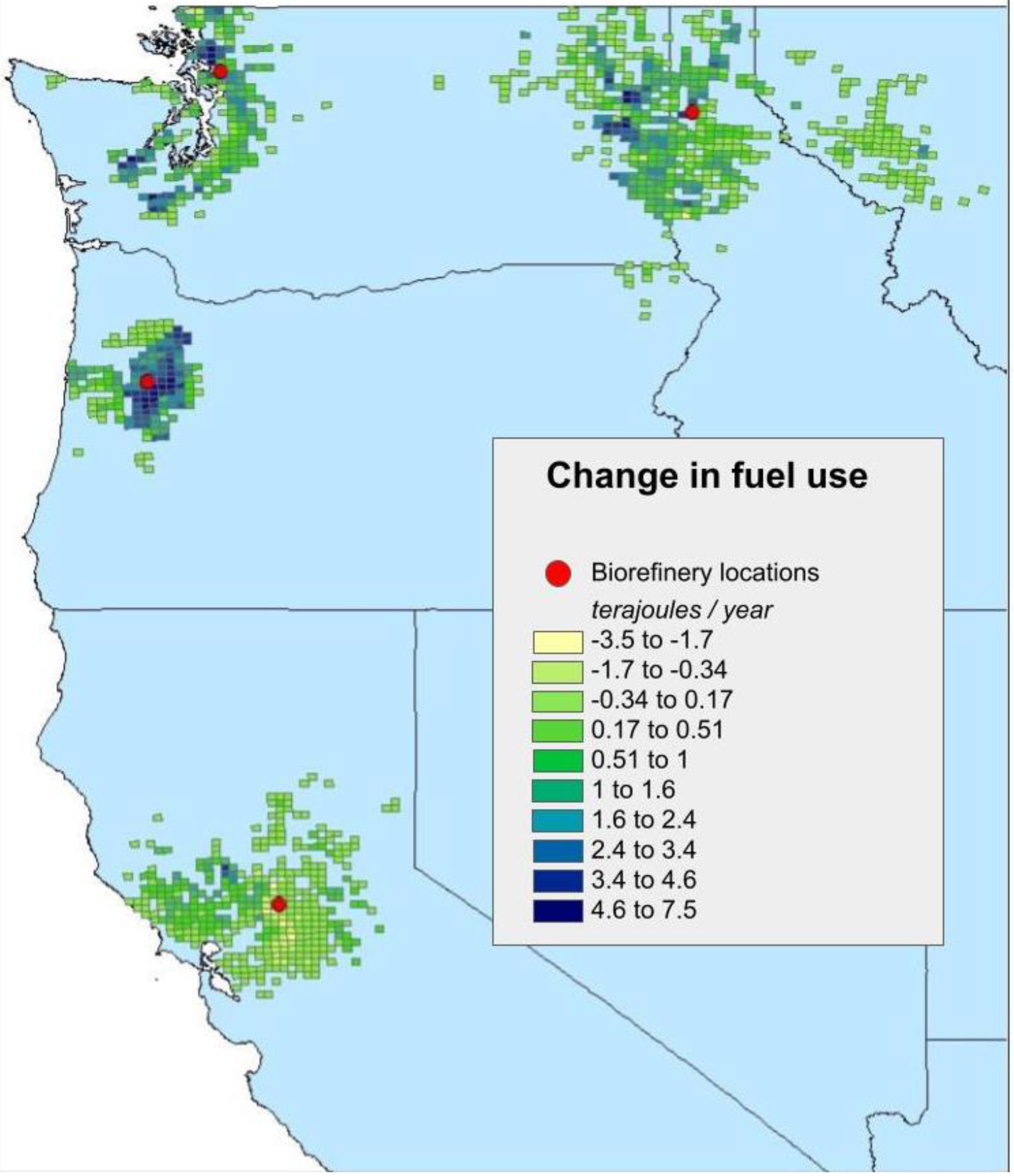
The use of mechanical equipment, with its associated fuel usage, is required for the management of both current croplands and poplar tree farms (
Table 8). Under current management practices, the Hayden region sees the highest annual fuel use, followed by Clarksburg, Pilchuck, and Jefferson. The average rate of use per hectare of cropland the fuel use is highest in the Clarksburg region while the average rate of fuel use is lower and fairly consistent in the other three regions (
Table 8). Switching to a poplar tree crop results in a fuel use increase for all four regions, with Jefferson seeing the highest increase (1582%), followed by Pilchuck (289%), Hayden (181%), and Clarksburg (28%). The average rate of fuel use per hectare of land when growing poplar is approximately the same for all four regions (~3.7 MJ of fuel use per hectare per year). Compared to the average rate of fuel use for the actively managed crops, the average rate of use per hectare to produce poplar is somewhat similar. The increase of actively managed lands when switching from the current practices to poplar production results in higher fuel use for each region. See
Figure 6 for a spatial visualization of the change of fuel use for each region.
Transportation distances from poplar tree farms to their respective biorefinery in each region are modelled using GBSM. The total distance and average distance of the poplar chips, which must travel annually from farm to biorefinery, differ for each region, as shown in
Table 9. Poplar chips travel the furthest in the Hayden region, followed by Clarksburg, and Jefferson. The distances traveled affect fuel needs to transport fuels and, the combustion of these fuels ultimately affects the total energy needed to produce bio-jet fuel, as well as the GWP. Fuel use for poplar chip transportation for each region is reported in
Table 9.
GWPs for lands identified in this study, and the changes in their management/use, for all four regions, are reported in
Table 10. Under current land management practices, Clarksburg has the highest GWP, followed by Hayden, Pilchuck, and Jefferson. The largest source of GHGs contributing to the GWP of the four regions is the manufacturing and use of nitrogen fertilizer followed by fuel use. Chemical inputs, phosphorus, and potassium fertilizers add relatively small amounts to the GWPs of current practices.
Switching to poplar production has varying GWP effects depending on the region. Poplar projections for Pilchuck, Hayden, and Jefferson indicate increases in the regional GWP by 40%, 137%, and 710%, respectively. Clarksburg GWP would decrease by 51% if land was switched to poplar production (
Table 10). When growing poplar, fuel use is the largest source of GHGs contributing to the GWP for all four regions, followed by nitrogen fertilizer manufacturing and N
2O emissions resulting from its use (
Table 10).
Direct land use change (DLUC) CO
2 emissions vary widely between the four regions, and are dependent on the amount (total hectares converted, not percentage of land converted) of rangeland converted to growing poplar. Regions with more rangelands converted to growing poplar have higher initial carbon debts that must be paid off. The highest DLUC emissions are in Jefferson with 3,400,000 tons of CO
2 eq, followed by Hayden at 3,300,000 tons of CO
2 eq, Pilchuck at 2,300,000 tons of CO
2 eq, and Clarksburg at 820,000 tons of CO
2 eq (
Table 11). These emissions contribute to the overall GWP for each region, but are one-time emissions, rather than related to annual emissions, as the other impacts discussed above. The DLUC therefore creates a carbon ‘debt’ that must be paid off before the respective regional biorefinery systems can become carbon neutral or negative. This is discussed in more detail towards the end of the discussion section.
4. Discussion
The amount and type of land converted to growing poplar trees for conversion to bio-jet fuel are dependent on multiple variables, including poplar crop yield, types of crops being grown in the region, and the amount of rangeland available. As demonstrated in
Figure 1 and
Table 2,
Table 3,
Table 4 and
Table 5, there is a wide variation in the amount and type of land converted in each region. These differences in land used to grow poplar trees dictate the differences in impacts observed in each region. Changes in fertilizers, chemical usage, and fuel use can have local impacts, as well as contribute to the overall GWP for each region. Understanding these site-specific characteristics are important to develop a more detailed view of how changes to land management practices can impact a region when land use is switched from current management practices to poplar bioenergy farms.
In the Hayden, Pilchuck, and Jefferson regions, the majority of land converted to growing poplar would come from rangeland, whereas the majority of land converted to growing poplar will come from croplands in the Clarksburg region (
Table 2,
Table 3,
Table 4 and
Table 5). Rangeland is assumed to be effectively unmanaged (no fertilizer, chemical inputs, etc.), and converting this land into active poplar crop management will increase the use of fertilizers, chemical inputs, and fuel use which lead to regional and global environmental impacts. Where actively managed crops are replaced with poplar production, the net effect to the land will vary, and is dependent on how those crops were managed prior to poplar conversion. For example, switching to poplar from crops that require more intensive management, such as grain corn, will result in a decrease in fertilizer use, chemical inputs, and fuel use. The displacement of food crops to produce bioenergy, and the potential observed benefit in reduction of fertilizers, chemical inputs, and fuel use, will likely add to the continuing debate of land use and food vs. fuels, however the analysis of indirect land use change and its overall impact is beyond the scope of this study.
Under current land management practices, nitrogen fertilizer use varied from region to region (
Figure 2). The amount of fertilizer applied per hectare of managed cropland depends on the region and the crops being grown there (
Table 6). Converting to poplar production results in a decrease in fertilizer use in all regions except Jefferson. Actively managed croplands in the Jefferson region do not have the lowest average amount of nitrogen fertilizer use per hectare (compared to active croplands in other regions), but it does have the lowest total amount of nitrogen fertilizer use for the lands that are converted to poplar. Jefferson is the only region to see an increase in nitrogen fertilizer use when switching to poplar production, because 93% of the land in the region that would grow poplar is currently unmanaged pasture/rangeland. Rangeland does not receive any fertilizer treatments. Growing poplar on this land, and adding nitrogen fertilizer, substantially increases the amount of nitrogen fertilizer use in the region, even though the average amount of fertilizer applied to a hectare of land for poplar is less than the average rate of application for current actively managed croplands (
Table 6). In the Clarksburg region, the opposite effect is observed. A majority of the land projected to grow poplar is currently being used as cropland to grow corn and wheat (
Table 6). These crops require higher nitrogen fertilizer use compared to growing poplar. Making the switch to poplar decreases the average amount of nitrogen fertilizer used per hectare and the total amount of nitrogen fertilizer used in the region. Both Pilchuck and Hayden regions see similar effects of decreasing nitrogen fertilizer use when switching to poplar, however the amount of tons of nitrogen saved varies per region (
Table 6).
Figure 2 displays the change in nitrogen fertilizer use and demonstrates the variability that exists region by region, and pixel by pixel. Even within a region, there is a large range of variability, with some pixels seeing an increase and others seeing a decrease. Phosphorus and potassium fertilizer use show similar trends within the regions for current croplands. Both of these fertilizers are applied at lower rates than nitrogen fertilizer, and their use does not differ as much within each region (
Table 6,
Figure 3 and
Figure 4). GreenWood Resources has indicated that they do not expect to use either of these fertilizers to grow poplar trees. Converting to poplar production cuts the use of potassium and phosphorus use in each region to zero. The discontinued use of these fertilizers reduces the impact associated with their production and use, but these do not have as big of an impact as the changes in nitrogen fertilizer use.
Chemical inputs used to control pests and promote crop growth (i.e., pesticides, herbicides, insecticides, etc.) vary from region to region (
Figure 5). Jefferson, Hayden, and Clarksburg regions are all expected to see increased use in chemical inputs when switching land use to poplar production (
Table 7). Similar to the use of nitrogen fertilizer, Jefferson will see the largest increase in chemical inputs, as much of the land converted to poplar is currently unmanaged. Under currently active practices, the Hayden region has the highest use of chemical inputs, and under a poplar management plan, the region is still expected to use more than all other regions combined. This trend shows that, compared to the other regions, the Hayden region is more susceptible to negative pest interactions, and therefore a higher use of chemical inputs is required to maintain good crop yields. Pilchuck is the only region projected to have a decrease in chemical inputs when lands are converted to poplar production. Compared to other regions, croplands in the Pilchuck region have the highest application rate per hectare of land (average rate, not total use) (
Table 7). However, when switched to poplar production, this region is expected to have the lowest average rate of use per hectare of land. A substantial decrease in chemical use comes from the northern area of the Pilchuck region, and this location is also predicted to see the largest decrease in fertilizer use as well, indicating an area of concentrated farmland that could switch to growing poplar and have a substantial effect on the region as a whole (
Figure 5). Observing the variation in
Figure 5 shows that there are differences in chemical use from pixel to pixel in each region, but the variation is much more pronounced in the Pilchuck and Hayden regions vs. the Clarksburg and Jefferson regions.
The average fuel use per hectare of current actively managed land is fairly consistent across all four regions, with Clarksburg seeing the highest fuel use (
Figure 6). Total regional fuel use is directly related to the amount of land in cultivation, and current fuel use for each region is consistent with this trend (
Table 8). Jefferson has the least amount of land in cultivation, followed by Pilchuck, Clarksburg, and Hayden (
Table 2,
Table 3,
Table 4 and
Table 5), and total regional fuel use follows this same progression. The estimated fuel use for poplar management is expected to be the same regardless of region, and all regions will see an increase in fuel use, as more lands start to grow poplar. As observed with nitrogen fertilizer use and chemical inputs, Jefferson has the highest increased fuel use, as 93% of the land to grow poplar will come from previously unmanaged lands. The variation of fuel use varies pixel by pixel in each region (
Figure 6). Much of this variation is accounted for by the amount of land in each pixel under cultivation when switching to poplar production. For some areas, like the central Clarksburg region, fuel use could actually decrease as croplands are switched from fuel-intensive crops (i.e., corn) to growing poplar (
Figure 6).
The GWP for each region is affected by fertilizers, chemical inputs, and fuel use, as well as the type of land converted to growing poplar. This results in a wide range of GWP values between the four regions (
Table 10). Expected poplar yield and land use have been identified as key factors that determine the amount of inputs and land needed by region to produce poplar. The lower the expected poplar yield per hectare, the more land required to be converted to growing poplar to meet biorefinery feedstock demands. The more land used, the more inputs required, and therefore the higher the regional GWP. Clarksburg requires the least amount of land to meet biorefinery needs, and therefore has the lowest GWP. Jefferson and Pilchuck have relatively similar total land needed, and have similar GWP. Hayden requires the most land and has the highest GWP. Looking at GWP alone though, does not tell the whole story when addressing the regional effects of feedstock growth and harvesting. The GWP savings must be evaluated to determine if a change in crop/land use results in an increase or decrease in regional GWP values. Tradeoffs in current land management practices, as well as direct land use change, factor into calculating the net effect on GWP for each region, and these items are discussed below.
Compared to current land use practices, Jefferson, Hayden, and Pilchuck regions would all see increases in GWP when switching to growing poplar (
Table 10—‘Farm Gate Total’). GWPs discussed here are for cradle-to-farm gate, and do not include transportation. The GWPs of poplar production with transportation to biorefinery are discussed further below. The increases in GWP are largely driven by a substantial increase in fuel use in each of these regions. Growing and harvesting poplar trees require considerably more fuel than current farming operations, and even more so than leaving the land unmanaged (i.e., converting rangelands to grow poplar). The Jefferson region is predicted to see a GWP increase of 710% as a result of both increased fuel use and fertilizer use, compared to leaving the land in its current management state, almost entirely unmanaged rangeland. Although the fuel use is predicted to increase in the Clarksburg region when converting to growing poplar trees, the GWP will be lower compared to current land management practices. The decrease in Clarksburg GWP is a result of the reduction in regional fertilizer use (
Table 10). From a GWP standpoint, the Clarksburg region sees the largest benefit in GHG reduction through the most efficient use of land (highest poplar yield) and through the conversion of high fertilizer input crops to lower fertilizer use for poplar production. If the goal of this study was to select one of the four regions to locate a biorefinery (rather than a regional assessment of each area), it would be difficult to select a location other than Clarksburg.
Delivering poplar chips from the farm gate to the respective biorefineries is not without its impacts, and there is variability between the four regions. Transportation distances are directly related to the poplar crop yields and land availability in each region. In regions where the annual poplar yield is projected to be lower, more hectares of land must be used to meet the yearly biorefinery feedstock needs. As more lands are converted to growing poplar, transportation distances from the farms to biorefinery also increases. The availability of farmland and pasture/rangeland at a selling price of USD 60/ton also has an effect on transportation distances. If less land is locally available to grow poplar trees, then lands at farther distances will be used to grow poplar. These issues are demonstrated in
Figure 1. The Jefferson region has a substantial amount of land available near the proposed biorefinery location (
Table 9). In the Hayden region, the opposite is observed, and the projected poplar yield is the lowest of the four regions, so more lands must be used to meet biorefinery feedstock needs; farm-to-biorefinery transportation distances increase. As transportation distances increase, so does the fuel needed to operate the delivery trucks, and ultimately the emission of greenhouse gases and other associated tailpipe emissions (
Table 9—‘Transportation to biorefinery’). Within the distances traveled (
Table 9), and associated emissions (
Table 10—‘Transportation to biorefinery’), there is variability between the four regions. Many biofuel LCA studies have assumed feedstock transportation distances of 100 km one way [
1]. One-size-fits-all models for transportation distances used in these studies may not accurately portray the effect of transportation in a region, by either overestimating the farm to biorefinery transportation distances (i.e., the Jefferson region) or by underestimating it (Hayden and Pilchuck regions). However, if regional data are not available, an average one-way transportation distance of 100 km could be considered a reasonable assumption, as this is about the average of all four locations.
An additional consideration when assessing GWP savings is the effect of direct land use change, which has a much more notable effect in regions where higher amounts of rangeland are converted to growing poplar (
Table 11). Rangeland conversion shows much higher greenhouse gas emissions than those already in annual crop rotations. This initial carbon ‘fee’ or ‘debt’ associated with clearing lands has the potential to substantially increase greenhouse gas emissions associated with transitioning land use, and can further influence regional GWP, and GWP savings. Not unexpectedly, the Jefferson GWP sees the biggest impact from DLUC, followed by Hayden, Pilchuck, and lastly, Clarksburg. As discussed above, based on the GWP of the four regions (
Table 10), only Clarksburg shows a decrease in greenhouse gas emissions, and therefore is the only region in which GWP savings are created when switching from current land management to a poplar bioenergy crop. With these GWP savings, Clarksburg would be the only region in which the DLUC emissions debt could be ‘paid back’ (the point at which the difference in annual emissions between current land management practices and a poplar growth and harvesting system becomes greater than the GWP generated from the DLUC). The GWP savings of Clarksburg could repay the DLUC carbon debt in 34.7 years. However, as discussed further below, the production of poplar is not the end point of this process, and addressing the entire life cycle of the production of bio-jet fuel is necessary to fully understand the relative scale of the feedstock production process and the calculation of DLUC carbon debt payoff.
The GWP of poplar production is only part of the greenhouse gas picture, and the GWP of feedstock production needs to be assessed in relation to the GWP of the biorefinery operations. Budsberg et al., 2016 [
15] reported the annual cradle-to-grave life cycle GWP for producing bio-jet fuel from poplar biomass. The annual GWP was found to be 710,000 tons of CO
2 eq from the production, and use 380,000,000 liters of bio-jet fuel (reported in Budsberg et al., 2016 [
15], as 54 g of CO
2 eq per MJ of bio jet). Direct land use change may be subtracted from the GWP values reported in Budsberg et al., 2016 [
15] to make direct comparisons with the work presented in this manuscript. Of the 710,000 tons of CO
2 eq, 76,000 tons of CO
2 eq (11% of the net GWP) were from the growth and harvesting of poplar biomass. The feedstock GWPs reported in this manuscript are lower than feedstock GWP reported in Budsberg et al., 2016 [
15]. This is due to newer poplar feedstock production practices that were developed in response to regional conditions at the GreenWood Resources pilot locations. Inserting the regional poplar growth and harvesting data into the full bio-jet fuel life cycle can help to complete the bigger picture of the regional effect on life cycle GWP. The full life annual cycle net GWP for each region would be 650,000 tons of CO
2 eq from Clarksburg, 660,000 tons of CO
2 eq at Pilchuck, 670,000 tons of CO
2 eq at Jefferson, and 690,000 tons of CO
2 eq at Hayden. The difference between the four regions is 40,000 tons of CO
2 eq, or about 4%. In comparison to the net life cycle GWP for an equivalent amount of petroleum-based jet fuel (380,000,000 liters), the GWP reductions for each region would be 47% at Clarksburg, 46% at Pilchuck, and Jefferson, and 44% at Hayden. The annual net GWP savings when replacing petroleum based jet fuel would be 570,000 tons of CO
2 eq at Clarksburg, 560,000 tons of CO
2 eq at Pilchuck and Jefferson, and 540,000 tons of CO
2 eq at Hayden. When looking at the complete life cycle for bio-jet fuel, we observe relatively small differences in the overall net GWP and large GWP savings that can be attributed to each region where poplar is grown and converted to fuel. The substantial amount of entire life cycle GWP savings can easily ‘repay’ the increase in carbon emissions when switching from current land management practices to growing poplar for biofuels.
Inserting DLUC back into the full LCA analysis of each region, these carbon savings can also be used to address the change in carbon debts that are estimated to be accrued in each region by converting land to growing poplar. All regions show that they will be able to repay the carbon debt accrued from DLUC from 1 to about 6 years. Clarksburg could repay the carbon debt in 1.4 years, Pilchuck in 4.1 years, and Hayden and Jefferson each in 6.1 years. For comparison, when DLUC is factored back into the original study in Budsberg et al., 2016 [
15], the carbon debt could have been repaid in 6.4 years. In other words, bio-jet fuel produced from poplar in the Clarksburg region could be considered carbon neutral (and then carbon negative compared to petroleum-based jet fuel) after 1.4 years, Pilchuck after 4.1 years, and Hayden and Jefferson after 6.1 years, when considering the impacts of DLUC.
The regional differences observed in this study further reinforce the need to develop more region-specific LCAs of biofuel systems. As noted by previous research, spatially oriented LCAs can help in identifying potential local impacts [
10,
11], areas for improvement or strategic implementation [
12], and regional comparisons [
11,
14]. Understanding regional differences and impacts at the local level can aid decision making processes that can help reduce risk of developing a new fuel system that would continue to exacerbate climate change, or create new environmental impacts within local communities. However, as noted in this study and in others, as we start to look at land use management changes with more granularity, there will need to be further discussions regarding tradeoffs in crop selection [
10,
11], biodiversity [
11], soil carbon [
14], greenhouse gas emissions [
12], and resiliency/adaptation to climate change.


