Abstract
Silver fir trees have cycles of low and high seed production, and thus it is necessary to collect seeds in high production years to save them for low production years to ensure the continuity of nursery production. Tree seeds can be stored loosely in piles or containers, but they need to be checked for viability before planting. The objective of this study was to find a quick and inexpensive method to determine the suitability of seed lots for planting. The working hypothesis was that an electronic nose device could be used to detect odors from fungi or from decomposing organic material, and thus aid in determination of whether seeds could be sown or discarded. To affirm and supplement results from the electronic nose, we used gas chromatography–mass spectrometry (GC-MS) to detect volatile secondary metabolites such as limonene and cadienes, which were found at the highest concentrations in both, infected and uninfected seeds. Uninfected seeds contained exceptionally high concentrations of pinene, which are known to be involved in plant resistance responses. Statistically higher levels of terpineol were found in infected seeds than in uninfected seeds. A prototype of our electronic nose partially discriminated between healthy and spoiled seeds, and between green and white fungal colonies grown on incubated seeds. These preliminary observations were encouraging and we plan to develop a practical device that will be useful for forestry and horticulture.
1. Introduction
The sustainability and biodiversity of forests depend on the quality of stock from forest nurseries. In Poland, foresters plant approximately half a billion seedlings every year based on the production of 800 million seedlings per year. Forecasts by the National Forest Cover Increasing Program assume an increasing the forest cover level from a current 30% to 33% by 2050 [1]. This will require the afforestation of millions of hectares and the availability of huge quantities of viable seed for sowing in nurseries. Currently, forest nursery seed is sent to seed stations, where quality is determined based on batches of 400 germinated seeds. However, this method is labor- and time-consuming, and seed must be sent well in advance. What is lacking is a quick and efficient method of assessing the seed suitability for sowing. Automated devices such as electronic noses may be useful for quicker assessments on a large scale. These devices have already been used to assess food quality. Human noses can be very sensitive to odors [2], and these abilities have developed during evolution to decrease the risk of consuming something that might be harmful. Odors can be emitted before fungal hyphae are visible on a plant surface and becomes visible to the naked eye. A seed may be non-viable due to damage or infection, but this is often not noticeable for seeds stored in dry conditions. Superficial visual inspection would not reveal the lack of viability which becomes apparent after seeds are sown and seedlings fail to emerge. We would like to develop a quick and efficient method to detect whether a seed sample is healthy and suitable for sowing or spoiled and should be further examined or discarded.
Since the introduction of the concept of an electronic nose [3,4,5], which is a device consisting of an array of nonspecific gas sensors, equipped with machine learning pattern recognition algorithms, various applications of this rapid and non-invasive diagnostic tool have been proposed. Several reports review potential applications, challenges, and possible improvements of electronic noses in focusing on forestry and agriculture [6,7,8,9,10,11]. Applications of electronic nose for detection and identification of fungal species were reviewed by Mota et al. [12]. Volatile organic compounds (VOC) emitted by various seeds infected by fungi have been analyzed with the help of electronic noses, including fungal contamination of cereal grain samples [13,14], rice [15], and rapeseed [16,17].
The purpose of this research was to examine seeds of silver fir (Abies alba) for viability via detection of degradative organisms via their VOC’s using an electronic nose. Silver fir is one of the main forest-forming species in Poland and is typical of the mountainous regions of central and southern Europe [18], but it is threatened by climate change and increasing pest pressures such as bark beetles.
2. Silver Fir in the Białowieża Forest
There are only two known countries in Europe where silver fir grows naturally in low-lying areas: France (Normandy) and Poland (Yata, Topór, Mienia, Rudka, and Tisovik reserves) [19,20,21,22]. Forests growing in the lowlands dominate in Poland at 84.8%, while the area of mountainous forests is 8.5% [23].
For almost 200 years, there has been a decline in wood resources and the area occupied by silver fir in European forests, known as the phenomenon of “the decline of silver fir in its natural range” [24]. According to some studies, the period of stagnation in some regions of Europe (Serbia) reaches 330 years [25]. It is assumed that this phenomenon was caused by a whole complex of biotic and abiotic factors, including the influence of humans [18,22,24]. However, the actual cause remains unclear to this day. Since 1981–1989, there has been a positive trend in the status of silver fir stands both in Poland and throughout Europe, which has improved significantly [24,26].
In the Belarusian part of the Białowieża Forest (which means wider forest) is the Tisovik tract (until 1939, called Cisówka), which is of˙ interest because of two crucial circumstances: (1) this is the northernmost “island” of autochthonous silver fir growing in the lowlands (120 km from the nearest natural stand in the Jata Reserve) [27,28,29]; and (2) the only currently surviving relict population of A. alba is present in the Tisovik tract, which is a part of the Białowieża Forest, one of the largest forest areas in Central and Eastern Europe [30,31]. For various reasons the silver fir population has never been large. From 1823 to World War II the number of silver fir trees fluctuated between 100 and 300 [32]. Currently only about 20 mature trees remain (unpublished data).
In 1922, Wiśniewski [33] found another very small group of silver fir trees in the Hubar tract, of the Białoweieża Forest. According to the researcher, it was undoubtedly of natural origin. As we learned from the oral communication of colleagues from the National Park “Belavežskaja Pušča” (Belarus), this fragment has not survived.
According to Środoń [34], who based, based his information on Wiśniewski [33], the oldest silver fir tree, blown down by the wind in Tisovik in 1924, had a trunk circumference of 120 cm and a height of 33.5 m, corresponding to an age of at least 250 years. This means it became established in the second half of the 17th century. This tree was a descendant of a silver fir which began to produce seeds at about 70 years of age [35]. Consequently, the beginning of the female parent’s life of this 250-year-old tree was at the end of the 16th to the beginning of the 17th century. Thus, based on these estimates, the age of the silver fir population in Tisovik is over 400 years, but is likely much longer. As noted by Paczoski [28], the appearance of silver fir in the Forest dates back to the climatic optimum of the Holocene.
Such long preservation in the Forest of this unique stand, first described in 1829 by Górski [27], and then studied in detail by Paczoski [28], allows an assumption that particular genetic traits allowed for survival. However, it has often been suggested that this is a consequence of a favorable location, i.e., a small sandy island covered with forest on the watershed in the middle of impassable swamps and watercourses, which provided high air humidity and frequent indirect precipitation (dew, frost) [32], as well as a high level of groundwater. However, for more than half a century now, those swamps have undergone senescence and infill, and the level of the groundwater has dropped significantly. Tisovik, currently does not have favorable hydrological conditions for silver fir [36] and is at the extreme northern end of a range which allows silver fir to regenerate naturally [32].
This unique relict population may have highly suitable genetic properties [37] and is a promising source of seed and vegetative material. Thus, it can be used in practical forestry outside the mountainous part of the range of the studied species, and not only in the Białowieza Forest region, but in other parts of Poland first of all in the natural forest region Mazury-Podlaskie (II).
This situation becomes especially important and relevant against the background of the current mass extinction of Norway spruce (Picea abies), especially in the northeastern part of its range [38,39]. The modern range of silver fir in Poland began in the sub-Boreal period of the Holocene and ended about 2000 years ago in the sub-Atlantic [34,40]. However, in the postglacial or in the so-called Little Ice Age (1300–1850), which came after the climatic optimum of the Holocene (about 800–1300 BP), Norway spruce (Picea abies), a typical boreal species, displaced the silver fir, growing in admixture with the main species [28].
Now, under conditions of global warming, only silver fir, which is similar to P. abies in terms of ecological and biological properties, can be a possible alternative to this species. We have already mentioned the favorable growth conditions for the silver fir in Tisovik, and this area was the source of seeds for our study [41], as well as from two other artificial silver fir stands of unknown geographical origin in the Polish part of the Białowieża Forest, but of an older age [42].
It is known that one of the main stresses faced by A. alba is low winter temperatures [18,35]. According to the predictive model of Vitasse et al. [43], under the conditions of modern climate, silver fir in Europe is favored, as predictions are for warming characterized by a sharp increase in winter temperatures with a constant amount of precipitation [36,44]. Dyderski et al. [45] also came to a similar conclusion, and they classified A. alba as a “winner” while modeling the ranges of major European tree species by 2061–2080 and the level of threat they may face under different scenarios of climate change.
However, at present, there is still not enough silvicultural experience of silver fir in northern Poland [46], although, in the middle of the 20th century, it grew on small plots, at least in 22 forestry enterprises in the western and middle part of the Mazury-Podlaskie forest region of northeastern Poland [19].
A serious problem with efficient use of the germplasm of silver fir from Tisovik is that a low percentage of silver fir seeds can germinate. According to Korczyk [29,32], this ranges from 12.8% to 17.5%, which are rates similar to the 12.6% reported by Gonczarenko et al. [47] for the Tisovik population [47]. These authors also noted that this can vary from tree to tree (2.6% to 40.0%).
Another negative factor significantly affects the quality of silver fir seeds from Tisovik. According to Korczyk [29,32], the percentage of damage to mature seeds by the larvae of Megastigmus suspectus Bor., Resseliella picea Seitn., and Barbara herrichina Obr. is very significant, reaching the range of 62–77%. It is not unreasonable to assume that these pests have a complex of associates, represented by pathogenic fungi, capable of infecting seeds and other parts of trees.
A similar situation, for example, takes place with Siberian fir (A. sibirica Ledb.), which is related to A. alba. In recent years, it has been dying from the combined action of the ussuri polygraph (Polygraphus proximus Blandf.) and associated ophiostomatoid fungi [48,49]. According to Russian researchers, this biotic tandem represents a new threat to fir forests in Siberia and throughout Europe [48].
That is why it is so important to have a tool such as the electronic nose to assess seeds of silver fir. This will make it possible to determine the degree of their infection with pathogenic organisms quickly and take measures in advance to anticipate the influence of this negative factor, which can significantly reduce the germination rate of seeds. This will facilitate sufficient healthy planting material for a unique population of relict silver fir. The purpose of this research was to examine silver fir seeds for viability using an electronic nose and analyze the emitted VOC’s composition by the GC-MS method.
3. Materials and Methods
3.1. Seed Collection and Preparation
Cones were harvested on 20 September 2021 from one plantation of half-sib silver fir Abies alba (Hajnówka forest district (Wilczy Jar sub-District, compartment 416ad) with geographical coordinates of E 23°39′17″, N 52°42′33″ (Figure 1). These trees were established in 1996 from 4-year-old seedlings derived from seeds collected in 1992 in the Tisovik reserve (Belarus) of the Białowieża Forest [50]. There were 11 mother trees giving rise to half-sib families of undetermined paternity.
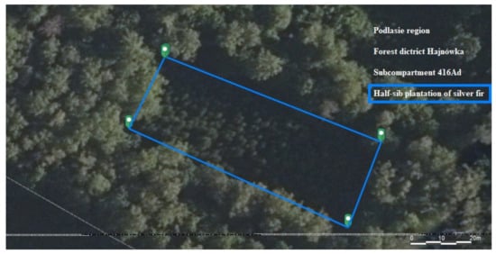
Figure 1.
Location of the area according to Forest Data Bank (https://www.bdl.lasy.gov.pl/portal/ accessed on 5 January 2022).
Seed production in plantations was observed for the first time in 2019, and in the next two years (2020, 2021) they were collected for sowing in autumn in the nursery of the Hajnówka forest enterprise, located in Białowieża Primeval. Cones were collected (20 September 2021), (Figure 2) and seeds were isolated from˙ cones (30 October 2021) (Figure 3). The seeds were stored at room temperature until experiments began (2 November 2021). The experiments were carried out using seeds of half-sib family No. 17. After collection, the cones were stored in a dry, well-ventilated room at a temperature of 20–25 °C, where they naturally dried. Artificial regulation of the photoperiod was not used. Under these dry conditions, it is less likely that the seeds have become contaminated by air spora which were able to establish.
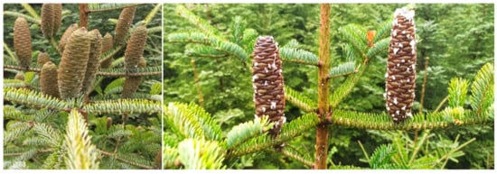
Figure 2.
Cones of silver fir trees from which seeds were collected in September 2021 (photo K. Wiłamowski). The cones ranged in length from 8.5 to 18.2 cm and width from 3.1 to 4.8 cm.
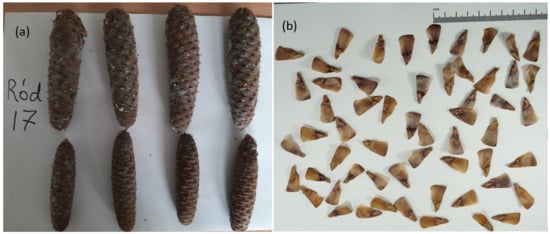
Figure 3.
Silver fir cones of a half-sib family N17 (a) (photo A. Marozau) and collected seeds (b) (photo K. Wiłamowski).
For the analysis of seed germination viability, a sample was taken from the fraction of clean seeds. Approximately 49 kg of the mixture of seeds with hulls dried at room temperature 20–25 °C were sent to the Kostrzyca Forest Gene Bank. From this mixture, 7.61 kg of pure seeds were obtained. X-ray analysis has been performed in Kostrzyca (Figure 4 to verify the quality of seeds and the presence of insects. A sample of 400 cleaned seeds, consisting of 4 replicates of 100 seeds each was tested [51] for germination dynamics and seed quality.
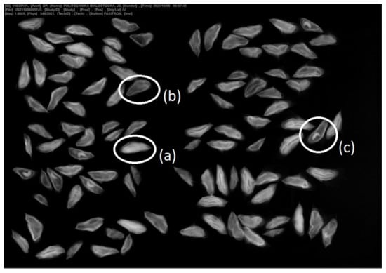
Figure 4.
X-ray pictures of silver fir seeds with the examples marked (a) correctly shaped, (b) empty, (c) insect larva (photo D. Polatowska, The Kostrzyca Forest Gene Bank).
Investigated seeds were surface sterilized by immersion in 75% propanol for thirty seconds and then rinsed with sterile distilled water for one minute. Six hundred seeds were chosen, and lots of up to 30 seeds were placed in 9-cm diameter Petri dishes on moist sterile paper towels. The plates were lidded but not tightly sealed. The papers towels were periodically moistened with sterile distilled water. Twenty Petri dishes were prepared in this way.
3.2. Fungal Selection and Identification
After incubation of the 20 Petri dishes with seeds, nine plates were selected for further investigation based on homogenous appearance, with similar fungal colonies appearing in the sets of plates. In addition to these plates, several other plates were selected for identification by subculturing and DNA sequencing. Genomic DNA was extracted from hyphae of three green and three white colonies. Then, genomic DNA was extracted using the NucleoSpin Plant II kit (Macherey-Nagel, Düren, Germany) according to the manufacturer’s instructions.
The region of the fungal internal transcribed spacer (ITS) was amplified with primers ITS1 (5-TCCGTAGGTGAACCTGCGG-3), and ITS4 (5-TCCTCCGCTTATTGATATGC-3) [52]. PCR was performed using the TaqNova- RED kit (BLIRT, Gdańsk, Poland). The 20 L PCR mix consisted of 10 µL 2X TaqNova- RED mix, 2 L 5 M of each primer, 2 L DNA extracts, and 2 L HO. Cycling was performed using a Veriti 96-well thermal cycler (ThermoFisher Scientific, Waltham, MA, USA) as follows: an initial denaturation step at 95 °C for 3 min, followed by 30 cycles (95 °C for 30 s, 55 °C for 30 s, and elongation at 72 °C for 30 s), and a final extension step at 75 °C for 5 min. Excess dNTPs and unincorporated primers were removed from the PCR product using CleanPCR (BLIRT, Gdańsk, Poland). DNA was eluted in 40 L HO. The amplified products were sequenced using the Sanger sequencing method in our laboratory.
Sequencing PCR reactions were performed using 1 L BigDye Terminator v. 3.1 Ready Reaction Mix (ThermoFisher Scientific), 2 L BigDye Sequencing Buffer (ThermoFisher Scientific), 1 L (5 M) ITS1 or ITS4 primer, and HO to bring the total volume to 10 L. The thermal profile for the sequencing reactions consisted of initial denaturation step of 96 °C for 1 min, followed by 25 cycles of 96 °C for 10 s, 50 °C for 5 s, and 60 °C for 105 s. The rDNA region was sequenced using an ABI 3500 xL genetic analyzer (ThermoFisher Scientific). For the sequences obtained a 98% alignment threshold over at least 440 base pairs was applied for species identification. Assignment of the obtained sequences to species was performed using the BOLDSYSTEMS identification engine [53,54].
3.3. Measurement of Volatile Organic Compounds
Volatile organic compounds (VOC) emitted from seeds were analyzed by headspace solid-phase microextraction coupled with gas chromatography and mass spectrometry (HS-SPME/GC-MS) following a previously used method [55,56] briefly described below.
In preliminary studies of VOCs emitted from asymptomatic silver fir seeds (control), divinylbenzene/carboxen/polydimethylsiloxane (DVB/CAR/PDMS), CAR/PDMS, and PDMS sorption fibres (Supelco, Bellefonte, PA, USA) were compared and DVB/CAR/PDMS fibre was selected for further research based on the highest effectiveness of the extraction–desorption cycle. Seeds for chemical analysis were selected at random, targeting those seeds with visible fungal growth. Seeds (1 ± 0.05 g, ~8 seeds) were placed in 60 mL glass vial with cap and septum (Büchi 049535) and heated at 40 °C for 60 min. SPME fiber was then added to the vial with a divinylbenzene/carboxene/polydimethylsiloxan stationary phase (Supelco, Bellefonte, PA, USA). The fiber was exposed to the headspace gas phase at 40 °C for 30 min. Immediately after exposure, the SPME fibre was inserted into an injection port of the GC-MS instrument for 10 min. GC–MS analyses were performed using an Agilent 7890A gas chromatograph with an Agilent 5975C mass spectrometer (Agilent Technologies Inc., Santa Clara, CA, USA). The injector was operated at a temperature of 250 °C in splitless mode. Chromatographic separation was performed on a capillary column HP -5MS (30 m × 0.25 mm × 0.25 m) at a helium flow rate of 1 mL/min. The initial temperature of the column was 35 °C and increased to 250 °C at a rate of 5 °C/min. The ion source and quadrupole temperatures were 230 °C and 150 °C, respectively. The electron impact mass spectra were obtained at ionization energy of 70 eV. Detection was performed in full scan mode for a range of 29–600 atomic mass units.
The peaks from the chromatogram were integrated, and the percentage of the components in the total ion current (TIC) was calculated. The mass spectral data and calculated retention indices were used to identify the components. Mass spectrometric identification was performed using the NIST (2020) and Wiley (2020) mass spectral libraries and the collections of Adams (2007) and Tkachev (2008) as well as a private, unpublished library of mass spectra, which had been created using standard chemical compounds. The retention indices of the analytes were determined considering the retention times of the n-alkanes. In a separate run, the mixture of C5C40 n-alkanes (1 L) was injected onto the chromatographic column and separated under the conditions previously described for GC–MS analyses of volatiles. Linear temperature-programmed experimental retention indices (RIexp) were calculated using the following expression RI = t t t t, where n is the number of carbon atoms in the alkane, t is the retention time of the analyte, t is the retention time of the n-alkane eluting immediately before the analyte, and t is the retention time of the n-alkane eluting directly after the analyte. The experimental retention indices (RI) were compared with those in the retention indices database (RI ) mentioned above.
3.4. Electronic Nose Measurements
3.4.1. Electronic Nose Device
The electronic nose used in these measurements was the PEN3 device (Airsense Analytics GmbH, Schwerin, Germany) [57]. It is a commercially available electronic nose, widely used in scientific laboratories, based on 10 metal oxide sensors that work only at high temperatures (about 350 °C and 500 °C). The sensors are sensitive to a wide range of gases, as listed in Table A1 in Appendix A. The unit has a very efficient air pump system with two inlets: one for the odor sampling and another for ambient air. The second is filtered through an activated carbon filter and is used as a reference signal level or to dilute the samples. The PEN3 was connected to a computer and controlled by Airsense WinMuster 1.6.2 software. It was also responsible for the acquisition of measurement data.
The measurement data of the PEN3 electronic nose were values or the conductivity of the sensors as a function of time when the sensors responded to the change in the chemical composition of the gas to which they were exposed. At the beginning of each measurement, the sensor matrix was purged with clean air, and then the air was pulled into the device, with a chamber flow rate of 7.7 mL/min. The values collected were unitless, as these were the magnitudes normalised by the baseline response of the sensor to clean air conditions measured just before the sensor was exposed to sampled air.
3.4.2. Samples Measurements
The electronic nose was turned on at least one hour before the measurement to ensure properly heated sensors. To ensure that no residue of old measurement samples remained in the sensor chamber, PEN3 automatically purges the sensors with filtered air for 180 s before starting the measurement. The zero point of the sensors was then measured, and during the next 120 s, the instrument recorded the response of the sensors to the constant flow of headspace gas from the measured sample. The sensor signals recorded by the software were G/G0. The conductance of the sensor during the measurement was divided by the conductance in ambient air.
The fir seed samples were kept in Petri dishes in which the infected seeds had been incubated (Figure 5). The number of seeds varied between individual samples, but in all cases the fungal hyphae covered approximately half or more of the seed surfaces in each 9 cm diameter Petri dish. We attempted standardize the samples by the amount of hyphal growth rather than by the number of seeds as we assumed that odor emission was related to hyphal growth. Variation in the amount of biological material in samples was an additional source of noise giving higher variability to the sensor signals collected by the electronic nose. This was related to the variability of the intensity of gases emitted by samples, but, to a lesser extent, to the chemical composition of the gases.
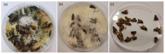
Figure 5.
Example of a Petri dish with fir seeds and mycelium covering the surface. (a) green, (b) white, and (c) uninfected/control samples. (photo M. Fasano, R. Tarakowski).
Immediately before measurements, the Petri dish to be measured was half-opened and the PEN3 electronic nose tube was placed near the center at 1 cm above a seed. The air above the seeds which should have contained volatile organic components emitted by the seeds and fungi, was pulled through the tube into the electronic nose device. In the interval between the 24-h measurements, the Petri dishes were kept closed and sealed with parafilm.
One or two measurements of each sample were taken every day. With two measurements per day, one series of measurements was performed in the morning and the second in the late afternoon to allow build up of VOC from the seeds. The order of samples in each series of measurement was randomized.
3.5. Analysis of Electronic Nose Data
In our experiments, 1200 units of data were collected in a single sample measurement since this corresponded to the number of readings of the sensor conductance within 2 min with a 1 s interval, multiplied by the number of sensors in the electronic nose device. The results of measurements collected during the experiment, discussed in Section 4.6.1, indicated the presence of measurement noise. We then preprocessed the data using the exponential smoothing method.
In our research, we used a subset of points from the smoothed curves for further analysis. First, we selected the response values between the 4th and 20th s in 2 s intervals. We also selected the values at the end of data collection at the 80th and 100th s. Thus, we obtained 10 features for each sensor. With this approach, we captured the main features of the overall sensor response due to the presence of the measured odor while significantly reducing the dimensionality of the problem. These features were then used as input for machine learning classification modeling.
Electronic nose measurements aim to use the collected data to build classification models capable of discriminating between the samples under study. This objective would make it possible to use such devices to detect the presence of odors in the environment and, in this way, evaluate the possibility of the presence of pathogens. For this task, we used a random forest model of machine learning [58].
Random forest is a popular machine learning algorithm used for classification tasks. It fits a number of decision tree classifiers on various sub-samples of the dataset and/or sub-samples of modeling features and uses averaging of the results. That approach allows to improve the predictive accuracy and control over-fitting.
3.6. Visualization of Distribution of Sensor Response Data
One of the random forest model outputs is a ranking of the most important features used for classification. In our analysis, we used these variables to visualize the distribution of the measured data in different ways. We compared the measured sensor response at a few characteristic moments of time elapsed from the beginning of sensor exposure to the measured gas. For such comparisons of distribution of data we used box-plot diagrams.
In addition, we transformed the modeling features using the principal component analysis (PCA) method. The PCA is one of the most commonly statistical techniques used for visualizing this type of data and allows us to gain some intuitive insights into the relationship between the patterns in the distribution of the data points. The input data for the PCA analysis methods are the sensor response magnitudes obtained at different time moments and possibly from different sensors. These values should not be directly compared when the data were collected from different sensors. The modeling features should be scaled to obtain the same variance for the PCA transformation. We used the top variables selected by the random forest model for the PCA transformation.
3.7. Data Processing and Analysis
All analyses of the data collected by the electronic nose measurements presented in this report were performed with Python 3.8 language codes, using statistical analysis methods from the scikit-learn module [59]. Processing and statistical analysis of data collected by the GC-MS measurements were performed using SAS 9.4 (SAS Institute, Cary, NC, USA) software using the SAS Enterprise Guide user interface and SAS/Stat procedures. PROC TTEST was used to verify statistical significance of differences in concentration of chemical components between uninfected and infected samples. Satterthwaite statistics, not assuming equal variance between groups, was used for calculation of p-value [60].
4. Results
4.1. Seed Collection
From 5.6 kg of seeds (each seed weighing 0.054 g) collected from the half-sib family No. 17, tested at the specialised laboratory in Kostrzyca, many did not germinate at all. The viability test of 400 seeds (after 14 days on wet filter paper at 20 °C) showed that seeds collected from half-sib family 17 in 2020–2021 did not exceed 19% viability, which is similar to previous data [29,47]. Seed viability varied between 10.7% and 19.0% per plate (Table 1).

Table 1.
Fruiting dynamics and seed quality analysis performed by the Seed Quality Assessment Station in Kostrzyca.
4.2. Preparation of Samples for Measurements
Twenty plates of up to 30 seeds each on wet paper toweling were incubated for 14 days at room temperature. After 14 days, fungal colonies appeared on some of the seeds. The developing mycelium covering the surface of seed took on a distinct green or white color, and these were chosen for electronic nose tests. From the Petri dishes covered in general with green or white mycelium and from control seeds (visually uninfected), 9 plates were selected for testing of volatiles with the electronic nose.
4.3. Fungal Identification of Hyphae from Seeds
We used amounts up to 30 seeds per plate, and there were likely different fungal species that grew out of the seeds, but there was often a dominant morphotype in each batch. We have made efforts to select only the plates where more than 90% of the seeds were covered with either white or green mycelium, although a few seeds in each plate may not have shown signs of infection. For sequencing we took incubated seeds from another 6 plates and obtained cultures form three green and three white colonies. DNA from three white colonies yielded three ITS sequences with 100% identity to Trichoderma harzianum (GenBank MK738148). ITS sequencing of DNA from three green colonies were found to belong to one of three species: Aspergillus baarnensis, Trichoderma koningii, or Xylaria ellisii (Table 2). The assignment of sequences obtained by the BOLDSYSTEMS Identification Engine to species was consistent with the results of the BLAST analysis.
Table 2.
Top BLAST match of six isolates to sequences in GenBank The colony name for the samples (G1–G3, W1–W3) are the same as those used in Table 3.
4.4. VOC Measurements
Fungal colonized seeds for each morphotype (green or white) were moved into 60 mL vials for gas measurements. The dominant chemical components identified by GC-MS from the six plates are shown in Figure 6. The source data used in this figure are listed in Table A3 in the Appendix A. This figure shows the average value of all samples and the average and standard deviation for the uninfected and infected seed categories. The limit of 1% of TIC gave 28 components that could be compared with the 130 chemical components identified in the samples by GC–MS, which meant that these represented 21.5% of the components in Table A2, in the Appendix A. These components represented 86% and 88% of TIC for infected and uninfected samples, respectively.
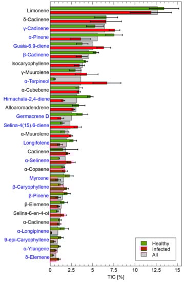
Figure 6.
Dominant chemical components identified by the GC-MS method. Comparison of two studies categories red–infected, green–uninfected. The standard deviation is presented as bar whiskers. The average of all samples is plotted as underlay grey bars. The components for which Total Ion Current (TIC) was higher than 1% are plotted. Blue component names indicate significant (p < 0.05) differences between uninfected and infected samples.
The most abundant substance was limonene, whose concentration differed slightly between uninfected and infected samples, but not significantly as shown by the standard deviation whiskers in Figure 6. Among the 28 components, the one that differed most greatly between uninfected and infected samples was -terpineol which was almost absent in uninfected samples. For other components whose relative content (% of TIC, Total Ion Current) differed between the categories, -cadinene, guaia6-9-diene, selina-4(15)6-diene, -selinene, -cadinene, -caryophyllene, and -elemene showed higher levels in infected samples and these differences were larger than the standard deviation bars between means of infected and uninfected samples. There were several components whose relative contents were significantly higher in uninfected samples including -pinene, -cadinene, himachala-2,4-diene, garmacrene D, longifolene, -pinene, and -longipinene.
Such visual data exploration provides interesting insights into the components that might help distinguish between the uninfected and infected samples. However, a statistical analysis using the t-test was also performed, with a goal to determine which of the chemical components identified by GC–MS measurements differed at the p-value level of 0.05 between uninfected and infected samples. In this case, the analysis was restricted to components with 1% of TIC as in the results mentioned earlier. This analysis of the GC-MS results aimed to assess chemical components that might help discriminate between uninfected and infected samples. In Figure 7, these data are presented in graphical form, where two factors are used. First, the difference in the amount of substance must be significant, which could be represented by the factor TIC avg_diff = TIC TIC. However, it is also important that this value is significantly different from the total amount of the component present in the sample, which can be defined as follows: TIC pct_diff = TIC avg_diff/2 TIC. The list of chemical elements presented in Figure 7 are included in Table A3 in the Appendix A. The full details of the results of the GC-MS measurements are listed in Table A5 in the Appendix A.
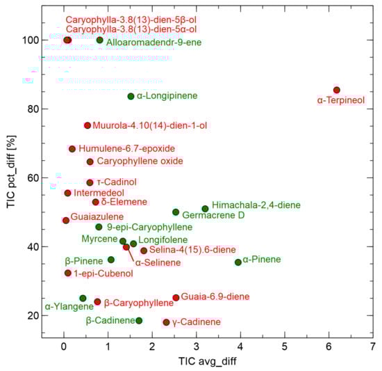
Figure 7.
Chemical components identified by the GC-MS method where relative amounts differed significantly between uninfected and infected samples. The x-axis presents absolute value of the difference of Total Ion Current (TIC) averages for samples categories (TIC avg_diff = |TIC–TIC). Sign of such difference, representing which samples category contain more of the component is indicated by the marker color: green = uninfected, red = infected. The y-axis represents the percent related to the average of TIC for all samples (TIC pct_diff = TIC avg_diff/2 TIC ).
4.5. Electronic Nose Measurements
During the experiments, 64 measurements were taken from three categories of samples (green, white and asymptomatic). The asymptomatic, non-fungal colonized batch of seeds were measured 18 times and the infected samples 46 times, but this group was treated as two categories of green and white samples according to the dominant color of the fungal colonies. Three samples of each category were used for the measurements, and the measurements were carried out for two weeks. The exact number of measurements is listed in Table 3. The numbers of measurements for various treatments differed, since in some cases measurements were interrupted, and we needed to wait for hours to allow VOC gases to accumulate inside the sealed Petri dishes.
Table 3.
Number of electronic nose measurements of the samples. C1–C3 are uninfected (control) samples, G1–G3 represent samples with green and W1–W3 samples with white fungi colonies.
4.6. Analysis of Data from Electronic Nose Measurements
4.6.1. Sensor Response
In Figure 8, we present the collected results of the measurements of VOC. The three categories studied are distinguished by colors, and we can visually detect some of the patterns that distinguish these samples. The sensor response curves are not smooth indicating high frequency noise present in the sensor signal during a single measurement cycle. This kind of noise could be reduced for further analysis using exponential smoothing method in the first phase of data preprocessing. There was also important variability of sensors response when we compare various response curves representing measurements of the same kind of sample but in different days of measurement. Such data variability has various sources as discussed in Section 5.3.
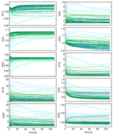
Figure 8.
Sensors responses as conductance normalized by the baseline value (G/G0), for measurements of studied samples categories C1–C3 (cyan), G1–G3 (green) and W1–W3 (blue). The sensor type is indicated as subfigures Y-axis labels.
Figure 8 showed stronger sensor response to the uninfected samples (C1–C3) compared to the infected ones. Furthermore, much higher variability was observed for the uninfected samples than the infected ones. There are also patterns in Figure 8, demonstrating differences between the signals of green and white samples. There was stronger response of the W5S, W1W, and W2W sensors when exposed to the G1–G3 (green) samples.
Figure 9 shows the distribution of the measurement points after transformation by principal component analysis. The top 10 features identified by the random forest binary classification model were used as input data for the PCA transformation. The list of the modeling features selected by the random forest models are presented in the following section.
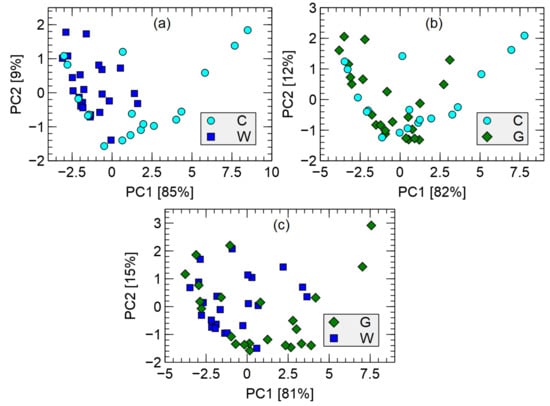
Figure 9.
Visualization of measured data in the Principal Component space, transforming the 10 the most important modeling features. Variability captured by the PC is indicated in axis labels. Comparison of C–uninfected, G–green, W–white samples. (a) uninfected vs. white, (b) uninfected vs. green, (c) green vs. white.
4.6.2. Classification Models
As described in Section 3.5, we used the collected data to build a machine learning classification model using the Random Forest method. In our experiments, we trained several models on the entire dataset and output the out-of-bag error to measure classification performance. This gave us an estimate of classification accuracy. In Figure 10, we show the results of this score as a function of the hyperparameter of the Random Forest model, the number of estimators. Separate models were compared for binary discrimination between all pairs of the three categories of samples considered. The accuracy reached values of 60% or higher, and the highest accuracy was obtained for the case of discrimination between two categories of infected samples (G-W) and reached a value just below 63%. The curves in this figure are relatively smooth, which is an indicator that the estimated accuracy was not due to fluctuations but reflected the data pattern.
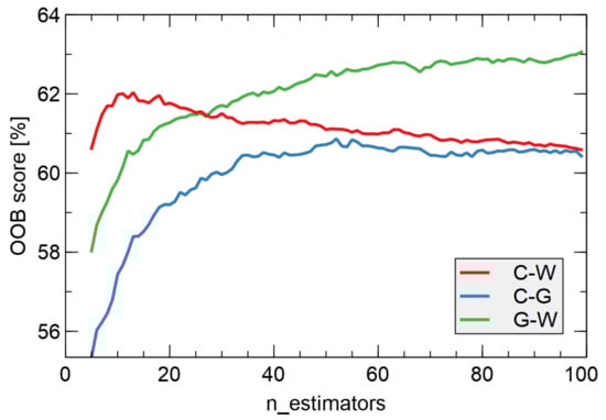
Figure 10.
Average of out-of-bag (OOB) error score (classification accuracy) versus the number of estimators used in training of the random forest classification model. Various binary models were compared: C-W–uninfected vs. white samples, C-G–uninfected vs. green samples, G-W–green vs. white samples. Since the number of observations varied between categories (Table 3), the OOB score was normalized to the case of equal populations in the classified categories.
One of the possible outputs from the random forest classification algorithm is a list of modeling features most often selected as important for classification, with their relative importance. We present these data in Figure 11, where the modeling features are sorted by their importance in classification model. As we have built individual binary classification models, there are separate lists of the features for each classification.
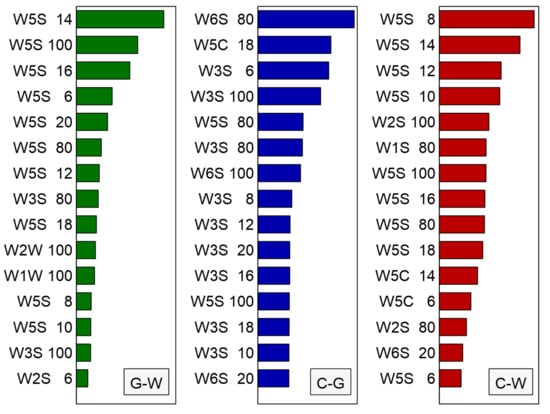
Figure 11.
Visualization of the top 15 the most important modeling features selected by the random forest classification method for three considered binary classifications G-W-green vs. white, C-G-control vs. green, C-W-control vs. white. The x-axis has no meaningful units. The name of each feature represents the symbol of the sensor (e.g., W5S) and the time (seconds, e.g., 14) of the measurement.
5. Discussion
5.1. Role of Chemical Components Identified by GC-MS Method
Based on the GC–MS analyses, we found that monoterpenes and sesquiterpenes were the main volatile components emitted from A. alba seeds. Previous studies found that essential oils from A. alba seeds contain a large amount of monoterpenes (especially limonene and -pinene) [61], whereas A. alba seed hydrolate is rich in sesquiterpenes [62]. Notable among the compounds was pinene (CH), the monoterpene responsible for the pine forest aroma. In addition to their occurrence in pines (Pinus spp.) and hemp (Cannabis sativa), and -pinene (as individual compounds or together) are also found in sage (Salvia spp.), mint basil (Ocimum menthaefolium), juniper (Juniperus communis), rosemary (Rosmarinus officinalis), French lavender (Lavandula stoechas), coriander (Coriandrum sativum), caraway (Cuminum cyminum), prickly juniper (Juniperus oxycedrus), tea tree (Melaleuca alternifolia), yarrow (Achillea millefolium), lovage (Ligusticum levisticum), strong dogwood (Grindelia camporum), black pepper (Piper nigrum), Korean mint (Agastache rugosa), and bergamot (Citrus bergamia) [63].
Like other terpenes and terpenoids, pinene is produced by the trichomes. It is one of the best-known members of the monoterpenes found in nature. This terpene has two isomers: -pinene and -pinene, each with two enantiomers. Pinene plays a protective role in defence against predators and pests, and - and -pinenes are used to manufacture liver and kidney medicines, as a flavor and fragrance additives, and as fungicides [64]. In a study of mice allergic to egg albumin, the use of -pinene reduced the number of nasal, eye, and ear abrasions, suggesting that this substance may be an effective anti-allergic agent [65].
In a study on -pinene [66], this compound showed similar efficacy to the drugs indomethacin and gabapentin. The researchers attributed the pain relief at least in part to the -pinene. Terpenes are produced by plants act as natural protection against pests and can be used to produce safe and effective pesticides including ones which contain -pinene, limonene, citronellol, camphor, and thymol among others [67]. and -pinenes are also used as antimicrobial agents, and in a study of pistachio gum essential oil, in which -pinene (75.6%) and -pinene (9.5%) were the two major constituents, the researchers found inhibitory activity against 9 of 13 bacteria and 3 of 3 pathogenic yeasts [68]. The presence of sesquiterpenes in VOC of incubated seeds is correlated with the detection of Trichoderma in such seeds. Emission of alloaromadendr-9-ene, -cadinene, germacrene D, and -selinene was reported in T. asperellum [69] longifolene and caryophyllene in T. longibrachiatum [70].
Resin accumulation in Pinaceae is induced after pathogen or herbivore attack and probably plays an important defensive role as a physical and chemical barrier against invaders [71,72,73]. Conifer resin contains mainly terpenes. Shifts in terpene blends and concentrations are strongly linked to tree stress and interactions with bark beetles and fungal symbionts. In healthy trees, oxygenated monoterpenes are represented only in trace amounts. However, after bark beetle attack and fungal inoculation, the concentration of oxygenated monoterpenes gradually increases via detoxification of monoterpene hydrocarbons in the beetle gut and by symbiotic fungi [74,75]. Thirty days after inoculation of Norway spruce (Picea abies) with the blue-stain fungus Ceratocystis polonica, the absolute amount and relative proportion of (+)-3-carene, sabinene, and terpinolene increased and (+)--pinene decreased [76]. Similarly, inoculation of Norway spruce with a blue-stain fungus, Endoconidiophora polonica, significantly increased monoterpenes, six sequiterpenes, and five diterpenes [77].
5.2. Chemical Components That Could Be Used for Detection of Infected Seeds
One of the goals of GC–MS analysis performed in our research was the identification of chemical components whose presence differed significantly between uninfected and infected samples, and which could be used for assessment of seeds quality by electronic nose measurements. Such information may be used in construction of the next generation of electronic noses, targeted to detect the spoilage of silver fir seeds, using sensors targeted to detection of specific identified VOC.
Figure 7 shows that -terpineol is the primary chemical component differentiating the studied samples. Among other components present in higher proportions in the infected samples, two other chemical also showed potential differentiation: guaila-6.9-diene and -cadiene, which showed significant levels of TIC avg_diff. All components whose presence differed between uninfected and infected samples at a p-value < 0.05 had a TIC pct_diff at 20% or higher. Interesting candidates for the indicators of infection could also be caryophylia-3.8(13)-diene-6 -ol and caryophylia-3.8(13)-diene-6 -ol, as they were detected only in the infected samples, but their relative content in VOC was very low, below 0.5% of TIC, which could be below the detection limit of other types of sensors. The components whose content was reduced in the infected samples could also be helpful for differentiation, and these were himachala-2,4-diene, germacrene D, and -pinene.
5.3. Electronic Nose Measurements
Unfortunately, as can be seen in Figure 8, there was considerable variability in the results, which could be due to variability in the biological sample sources or random noise, such as changes in environmental conditions, variability in the emission rate VOC of the samples, variability in the internal processes of the MOX sensors, etc. Even if the same Petri dish were measured several times but with a delay of one day, the samples were not exactly the same. We could observe development of fungi and hyphal growth over healthy regions of seeds or onto the paper lining so the samples differed. In other research with the PEN3 electronic nose device, similar problems in the repeatability of the measurement results have been found [78,79,80].
It might be helpful to look at the distribution of sensor response at specific time points and compare this value for the categories under study, using the usual box-plot visualization as shown in Figure 12. The PEN3 manufacturer recommends using as input for machine learning models data from the end of measurement, but in our analyses, we augmented it by data from the beginning of the response curve. After building the random forest models we verified what kind of features were most often selected and observed that indeed responses at the end of measurements were used but, even more often are selected measure points collected from the region of 14–20 s. The choice of 10, 14, 20 s for constructing this graph was arbitrary, with intention to show the main features of the data distribution.
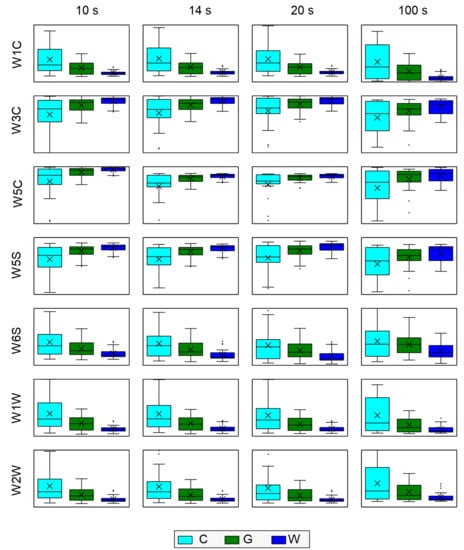
Figure 12.
Distribution of modeling feature extracted from the sensor response characteristics for measured samples categories. Data for selected sensors at the selected moment of measurements are indicated in the grid labels. The box spans the 1st to 3rd quantile of data. The whiskers span 1.5 IQR (IQR-inter quantile range). The horizontal line inside the box represents the median, and the × inside boxes represents the mean.
The distribution of sensor response is much more scattered for the uninfected samples (C1–C3) than for the infected samples (Figure 12). The distribution of signals from the uninfected samples overlapped with the distribution of signals from the infected samples, which causes low performance of samples classification using electronic nose data. The distribution of sensor signal level of G1–G3 (green) samples was significantly different from those of the W1–W3 (white) distribution but they overlapped. However, the median of the G1–G3 samples was remarkably far from the box that represented the bulk of the W1–W3 sample distribution (Figure 8). Moreover, the range of the G1–G3 distribution was much higher than that of the W1–W3 distribution, which can be explained by white samples containing only Trichoderma harzianum, and among the green samples, multiple species were detected and identified (Table 2).
5.4. Classification Modeling Using Electronic Nose Data
Various methods of extracting modeling features from sensors response curves can be found. The Airsense Winmuster software, provided with the PEN3 electronic nose, uses sensor response values at given time moments, usually at the end of observation. In many other reports, more advanced methods are used [81,82]. In our approach, we used the raw sensor response from various points in the response curve.
Here are some advantages of this method to justify the choice of the classification algorithm. In this method, a set of weak decision tree classifiers was trained with different subsamples of the whole training dataset and subsets of modeling features, and the partial results were averaged. This approach led to improved prediction accuracy of such a composite model. It is also essential that the random forest models are not prone to overfitting and are robust to the choice of model parameters, which is particularly important when a small number of training observations are used, as found in our study. Another advantage of this approach is the extraction of the so-called out-of-bag (OOB) error. This is the average error calculated using the predictions of the trees for observations that were not included in the particular bootstrap sample. This allows an entire dataset to be fitted and validated during a single training procedure [83]. Another vital advantage of the random forest method is the natural method of evaluating of the importance of modeling features, based on the frequency with which they enter the models.
The classification accuracy found here (63%) was similar to other results (64%) obtained for other biological samples [84], when a custom-made electronic nose was used to discriminate between two pathogenic oomycetes infecting germinated acorns. However, it was much lower than the accuracy (74–78%) obtained in our studies of odors of ash roots infected with Hymenoscyphus fraxineus, where we also used the PEN3 device [80].
5.5. Application of Electronic Nose
Results of studies using the electronic nose to discriminate between uninfected and fungal infected seeds are presented for the first time in this proof of concept study, and thus a limited number of biological replicates were used. We wanted to see if this direction of research was worthwhile pursuing. We used dead (killed by fungi) seeds and seeds without fungal growth after incubation, but the uninfected seeds also showed low germination rates which is typical for fir seeds, especially those produced outside the area typical for silver fir occurrence in Poland. Silver fir is normally found in the northwest and southern parts of the country [85], and the seeds for this study were from the northeast. However, it is important to study the seeds from the northeast because foresters hope to replace Norway spruce with silver fir in the Białowieża Forest, a remnant of the ancient forest which covered all of northern Europe. Near the Białowieża Forest, Norway spruce trees have been dying as a result of a bark beetle outbreak of unprecedented scale enhanced by climate change, which has killed the largest Norway spruce trees [39]. In our experiments, we used one of the leading commercially available electronic devices for measuring volatile compounds (electronic nose PEN3), and we follow the recommended measurement protocols. The results showed discrimination between the infected and non-infected seeds but with high variability in the results which indicates that the protocol and equipment are not currently suitable for field or practical use. Further research is needed, especially in the construction of special devices with sensors targeted to the chemical components in the types of biological samples studied, and improved methods of data analysis.
6. Conclusions
Foresters have to deal with the problem that many forest trees, such as firs and pines, produce seeds irregularly with larger seed set every 3–4 years, and for beeches and oaks, every 4–8 years. This makes it necessary to collect large quantities of seeds in bountiful “seed years” and maintain them during storage. Seeds must be maintained with some moisture to maintain high viability, but this allows for a risk of fungal infection with the moisture present. Therefore, nursery workers need to be able to quickly monitor both the storage process and the health status of the seeds on a large scale to decide whether the seeds are suitable for sowing and nursery production before the start of the growing season. The objective of this study was to find a quick and inexpensive method to assess the suitability of seed lots for nursery use without laborious methods of seed germination. The working hypothesis was that an electronic nose would detect the odor of fungi and/or decaying organic matter and thus help the seed manager decide whether the seed lot was suitable for sowing in plots or should be discarded. The experiment was conducted in vitro on uninfected and naturally infected Abies alba silver fir seeds. We found that the commercial, general purpose electronic nose device PEN3 was able to partially discriminate between uninfected and spoiled seeds.
The main conclusions from the presented research are as follows.
- (i)
- At the time of measurements, fungi of the genera Xylaria, Aspergillus, and Trichoderma were found on the damaged seeds.
- (ii)
- Electronic nose measurement data analyzed by the machine learning algorithms can be used as a tool for evaluation of the status of silver fir seeds stockage.
- (iii)
- Gas chromatography–mass spectrometry measurements can give valuable information concerning the chemical composition of the volatile organic components emitted by the spoiled seeds of silver fir.
- (iv)
- -terpineol seems to be the best candidate as a chemical marker of the health status of stored silver fir seeds and its significantly higher concentration may be an indication of fungal spoilage.
- (v)
- Construction of dedicated electronic noses with gas sensors targeted to specific chemical components present in volatiles emitted by fungi would be helpful to improve the performance of spoilage detection protocols.
Author Contributions
Conceptualization, T.O., P.B. and M.F.; methodology, T.O., M.T. and M.F.; software, P.B.; validation, P.B., R.T., M.F. and A.M.; formal analysis, M.S. and M.F.; investigation, M.F., T.M. and M.S.; resources, M.S. and A.M.; data curation, R.T. and M.T.; writing—original draft preparation, P.B., T.M., A.M. and M.S.; writing—review and editing, T.O., A.M. and T.H.; visualization, R.T., A.M. and P.B.; supervision, T.O., P.B. and M.T.; project administration, A.M.; funding acquisition, P.B. and M.S. All authors have read and agreed to the published version of the manuscript.
Funding
This work was partially supported by the National Centre for Research and Development by the grant agreement BIOSTRATEG3/347105/9/NCBR/2017.
Institutional Review Board Statement
Not applicable.
Informed Consent Statement
Not applicable.
Data Availability Statement
The data presented in this study are available from the corresponding author.
Conflicts of Interest
The authors declare no conflict of interest.
Appendix A. Sensors in PEN3 Electronic Nose Device
Table A1.
Sensor array details in PEN3 electronic nose device, as reported in the menu of options of the electronic nose software.
Table A1.
Sensor array details in PEN3 electronic nose device, as reported in the menu of options of the electronic nose software.
| Sensor | Main Gas Targets |
|---|---|
| W1C | Aromatic organic compounds. |
| W5S | Very sensitive, broad range sensitivity, reacts to nitrogen oxides, very sensitive to negative signals. |
| W3C | Ammonia, also used as sensor for aromatic compounds. |
| W6S | Detects mainly hydrogen gas. |
| W5C | Alkanes, aromatic compounds, and non-polar organic compounds. |
| W1S | Sensitive to methane. A broad range of organic compounds detected. |
| W1W | Detects inorganic sulfur compounds, e.g., HS. Also sensitive to many terpenes and sulfur-containing organic compounds. |
| W2S | Detects alcohol, partially sensitive to aromatic compounds, broad range. |
| W2W | Aromatic compounds, inorganic sulfur and organic compounds. |
| W3S | Reacts to high concentrations of methane (very selective) and aliphatic organic compounds. |
Appendix B. The Most Important Chemical Components Identified by the GC-MS Method
Table A2.
Dominant chemical components identified by the GC–MS method ordered by average over all measurements. Average and standard deviation for uninfected and infected categories. The components for which Total Ion Current (TIC) was higher than 1% are selected. The last line represent the coverage of the listed components comparing to the total ion current collected during the GC-MS measurements.
| Compound | TIC [%] | ||||
|---|---|---|---|---|---|
| All | Uninfected | Infected | |||
| Avg | Avg | Std | Avg | Std | |
| Limonene | 12.66 | 13.42 | 1.75 | 11.89 | 2.45 |
| -Cadinene | 6.59 | 6.61 | 1.35 | 6.57 | 1.83 |
| -Cadinene | 6.43 | 5.28 | 0.99 | 7.59 | 0.63 |
| -Pinene | 5.57 | 7.54 | 0.99 | 3.59 | 1.19 |
| Guaia-6.9-diene | 5.04 | 3.78 | 0.68 | 6.31 | 0.82 |
| -Cadinene | 4.56 | 5.41 | 0.31 | 3.72 | 0.65 |
| Isocaryophyllene | 3.84 | 4.23 | 0.21 | 3.44 | 0.60 |
| -Muurolene | 3.63 | 2.96 | 0.69 | 4.30 | 1.35 |
| -Terpineol | 3.61 | 0.52 | 0.10 | 6.70 | 1.65 |
| -Cubebene | 3.39 | 3.41 | 0.37 | 3.37 | 0.19 |
| Himachala-2,4-diene | 3.14 | 4.74 | 0.33 | 1.54 | 0.19 |
| Alloaromadendrene | 3.05 | 3.36 | 0.74 | 2.74 | 0.17 |
| Germacrene D | 2.53 | 3.80 | 0.65 | 1.26 | 0.35 |
| Selina-4(15)6-diene | 2.33 | 1.43 | 0.21 | 3.24 | 0.43 |
| -Muurolene | 2.11 | 1.74 | 0.48 | 2.48 | 0.19 |
| Longifolene | 1.93 | 2.72 | 0.39 | 1.14 | 0.29 |
| Cadinene | 1.79 | 1.47 | 0.46 | 2.11 | 0.20 |
| -Selinene | 1.77 | 1.07 | 0.02 | 2.48 | 0.48 |
| -Copaene | 1.66 | 1.55 | 0.17 | 1.76 | 0.28 |
| Myrcene | 1.60 | 2.27 | 0.44 | 0.94 | 0.29 |
| -Caryophyllene | 1.58 | 1.20 | 0.22 | 1.96 | 0.23 |
| -Pinene | 1.47 | 2.01 | 0.37 | 0.94 | 0.26 |
| -Elemene | 1.31 | 1.64 | 0.40 | 0.97 | 0.16 |
| Selina-6-en-4-ol | 1.23 | 0.85 | 0.11 | 1.61 | 0.35 |
| -Cadinene | 1.10 | 1.14 | 0.18 | 1.06 | 0.22 |
| -Longipinene | 0.91 | 1.66 | 0.50 | 0.15 | 0.03 |
| 9-epi-Caryophyllene | 0.87 | 1.26 | 0.28 | 0.47 | 0.13 |
| -Ylangene | 0.85 | 1.07 | 0.13 | 0.64 | 0.09 |
| -Elemene | 0.68 | 0.32 | 0.10 | 1.04 | 0.15 |
| Sum of the above | 87.23 | 88.46 | 86.01 | ||
Table A3.
Volatile Organic Components identified by the Gas Chromatography–Mass Spectrometry measurements. The average (avg) and standard deviation (std) of the percentage of the Total Ion Current (TIC) are calculated from repetitions of all studied samples measurements. Only components, which differs for two studied categories are listed (p-value below 0.05). Data are sorted by retention time (in minutes).
| Compound | Ret. Time | TIC | p-Value | |||
|---|---|---|---|---|---|---|
| Uninfected | Infected | |||||
| Avg | Std | Avg | Std | |||
| -Pinene | 8.503 | 7.54 | 0.99 | 3.59 | 1.19 | 0.0126 |
| -Pinene | 9.615 | 2.00 | 0.37 | 0.94 | 0.26 | 0.0181 |
| Myrcene | 10.062 | 2.27 | 0.44 | 0.94 | 0.29 | 0.0165 |
| -Terpineol | 15.995 | 0.52 | 0.10 | 6.70 | 1.65 | 0.0226 |
| -Elemene | 20.041 | 0.32 | 0.10 | 1.04 | 0.15 | 0.0037 |
| -Longipinene | 20.504 | 1.66 | 0.50 | 0.15 | 0.03 | 0.0335 |
| -Ylangene | 20.969 | 1.07 | 0.13 | 0.64 | 0.09 | 0.0114 |
| Longifolene | 21.970 | 2.72 | 0.39 | 1.14 | 0.29 | 0.0065 |
| -Caryophyllene | 22.239 | 1.20 | 0.22 | 1.96 | 0.23 | 0.0143 |
| Himachala-2,4-diene | 22.509 | 4.74 | 0.33 | 1.54 | 0.19 | 0.0005 |
| Guaia-6,9-diene | 22.905 | 3.78 | 0.68 | 6.31 | 0.82 | 0.0154 |
| Selina-4(15),6-diene | 23.139 | 1.43 | 0.21 | 3.24 | 0.43 | 0.0084 |
| 9-epi-Caryophyllene | 23.492 | 1.26 | 0.28 | 0.47 | 0.13 | 0.0253 |
| Germacrene D | 23.868 | 3.80 | 0.65 | 1.26 | 0.35 | 0.0089 |
| Alloaromadendr-9-ene | 23.911 | 0.81 | 0.17 | 0.00 | 0.00 | 0.0139 |
| -Selinene | 24.117 | 1.07 | 0.02 | 2.48 | 0.48 | 0.0355 |
| -Cadinene | 24.285 | 5.41 | 0.31 | 3.72 | 0.64 | 0.0285 |
| -Cadinene | 24.690 | 5.28 | 0.99 | 7.59 | 0.63 | 0.0349 |
| Caryophyllene oxide | 26.204 | 0.16 | 0.03 | 0.74 | 0.21 | 0.0354 |
| Humulene-6,7-epoxide | 26.780 | 0.04 | 0.01 | 0.23 | 0.07 | 0.0416 |
| Muurola-4,10(14)-dien-1-ol | 27.179 | 0.08 | 0.02 | 0.62 | 0.12 | 0.0152 |
| 1-epi-Cubenol | 27.282 | 0.09 | 0.01 | 0.19 | 0.02 | 0.0043 |
| -Cadinol | 27.469 | 0.21 | 0.05 | 0.80 | 0.11 | 0.0045 |
| Caryophylla-3,8(13)-diene-5 -ol | 27.766 | 0.00 | 0.00 | 0.10 | 0.03 | 0.0356 |
| Intermedeol | 27.904 | 0.03 | 0.01 | 0.12 | 0.01 | 0.0009 |
| Caryophylla-3,8(13)-dien-5 -ol | 28.357 | 0.00 | 0.00 | 0.07 | 0.01 | 0.0136 |
| Guaiazulene | 30.414 | 0.026 | 0.01 | 0.07 | 0.01 | 0.0043 |
Appendix C. Detail Results of the Gas Chromatography-Mass Spectrometry Measurements
Table A4.
Description of the columns in tables presenting the Gas Chromatography–Mass Spectrometry results.
Table A4.
Description of the columns in tables presenting the Gas Chromatography–Mass Spectrometry results.
| Column | Description |
|---|---|
| Compound | Group and name of the identified compounds. |
| CAS | CAS Registry Number. |
| m/z | Mass-to-charge ratio (fragmentation ion). |
| M | Molecular ion. |
| Time | Retention time. |
| RI | Experimental value of the Retention Index. |
| RI | Literature value of the Retention Index. |
| Area | Area of the Total Ion Current peak |
| TIC | Percentage of the Total Ion Current. |
Table A5.
The chemical components identified by the Gas Chromatography–Mass Spectrometry measurements. The meaning of columns is defined in Table A4.
Table A5.
The chemical components identified by the Gas Chromatography–Mass Spectrometry measurements. The meaning of columns is defined in Table A4.
| Compound | CAS | m/z | M+ | Time | RI | RI | Uninfected | Infected | ||
|---|---|---|---|---|---|---|---|---|---|---|
| Area | TIC | Area | TIC | |||||||
| Monoterpenes | 31,298 | 28.40 | 28,239 | 28.69 | ||||||
| Tricyclene | 508-32-7 | 93, 91, 77, 79, 92 | 136 | 7.980 | 918 | 921 | 27 | 0.03 | ||
| -Pinene | 80-56-8 | 93, 91, 92, 77, 79 | 136 | 8.503 | 933 | 932 | 8430 | 7.54 | 3493 | 3.59 |
| Camphene | 79-92-5 | 93, 121, 91, 79, 77 | 136 | 8.800 | 944 | 946 | 466 | 0.43 | 109 | 0.11 |
| Verbenene | 4080-46-0 | 91, 92, 93, 77, 79 | 134 | 8.925 | 949 | 952 | 30 | 0.03 | ||
| 3,7,7-Trimethyl-1,3,5-cycloheptatriene | 3479-89-8 | 119, 91, 77, 117, 134 | 134 | 9.391 | 967 | 970 | 14 | 0.01 | ||
| Sabinene | 3387-41-5 | 93, 32, 91, 77, 79 | 136 | 9.483 | 970 | 969 | 14 | 0.02 | ||
| -Pinene | 127-91-3 | 93, 41, 91, 79, 77 | 136 | 9.615 | 975 | 974 | 2293 | 2.01 | 908 | 0.94 |
| Myrcene | 123-35-3 | 93, 41, 69, 91, 79 | 136 | 10.062 | 990 | 988 | 2454 | 2.27 | 905 | 0.94 |
| p-Mentha-1,5,8-triene | 21195-59-5 | 119, 91, 134, 77, 92 | 134 | 10.428 | 1006 | 1005 | 66 | 0.07 | ||
| 3-Carene | 13466-78-9 | 93, 91, 77, 79, 92 | 136 | 10.576 | 1011 | 1010 | 948 | 0.98 | ||
| Limonene | 138-86-3 | 93, 68, 67, 79, 91 | 136 | 11.422 | 1029 | 1028 | 14,654 | 13.42 | 11,702 | 11.89 |
| -Terpinene | 99-85-4 | 93, 91, 77, 136, 121 | 136 | 12.215 | 1057 | 1054 | 79 | 0.07 | 20 | 0.02 |
| cis-Sabinenehydrate | 15826-82-1 | 93, 43, 71, 91, 121 | 154 | 12.288 | 1063 | 1065 | 15 | 0.01 | ||
| -Terpinolene | 586-62-9 | 93, 121, 91, 136, 79 | 136 | 12.925 | 1089 | 1086 | 594 | 0.53 | 86 | 0.09 |
| 1-Undecene | 821-95-4 | 55, 70, 56, 69, 41 | 154 | 12.980 | 1092 | 1092 | 402 | 0.38 | ||
| Linalool | 78-70-6 | 71, 43, 41, 93, 55 | 154 | 13.228 | 1101 | 1100 | 28 | 0.03 | ||
| Perillene | 539-52-6 | 69, 41, 81, 150, 53 | 150 | 13.452 | 1105 | 1002 | 14 | 0.01 | 21 | 0.02 |
| 1,3,8-p-Menthatriene | 18368-95-1 | 91, 119, 134, 105, 77 | 134 | 13.766 | 1109 | 1008 | 19 | 0.02 | ||
| trans--Thujone | 471-15-8 | 81, 41, 67, 43, 95 | 152 | 13.902 | 1119 | 1117 | 37 | 0.04 | ||
| trans-p-Mentha-2,8-dien-1-ol | 7212-40-0 | 91, 79, 109, 94, 43 | 152 | 13.987 | 1122 | 1121 | 30 | 0.03 | 93 | 0.09 |
| cis-Limonene oxide | 13837-75-7 | 43, 67, 41, 109, 79 | 152 | 14.259 | 1134 | 1133 | 95 | 0.09 | 128 | 0.12 |
| cis-p-Mentha-2,8-dien-1-ol | 3886-78-0 | 109, 91, 43, 79, 134 | 152 | 14.293 | 1137 | 1135 | 123 | 0.12 | ||
| trans-Pinocarveol | 547-61-5 | 55, 92, 91, 41, 70 | 152 | 14.411 | 1138 | 1135 | 41 | 0.04 | ||
| trans-Limonene oxide | 4959-35-7 | 43, 67, 94, 79, 93 | 152 | 14.482 | 1139 | 1137 | 46 | 0.05 | ||
| Camphene hydrate | 64474-11-9 | 43, 71, 41, 69, 86 | 154 | 14.531 | 1144 | 1145 | 93 | 0.09 | ||
| -Terpineol | 138-87-4 | 71, 43, 93, 69, 41 | 154 | 14.618 | 1148 | 1145 | 804 | 0.80 | ||
| Monoterpenoide CHO | n/a | 95, 81, 109, 41, 91 | 152 | 14.686 | 1151 | n/a | 100 | 0.09 | ||
| Pinocamphone | 547-60-4 | 83, 55, 69, 41, 81 | 152 | 15.141 | 1161 | 1161 | 53 | 0.05 | 67 | 0.07 |
| Pinocarvone | 16812-40-1 | 81, 53, 79, 108, 41 | 150 | 15.201 | 1163 | 1162 | 65 | 0.06 | ||
| Borneol | 507-70-0 | 95, 41, 110, 67, 43 | 154 | 15.215 | 1165 | 1165 | 170 | 0.18 | ||
| Isopinocamphone | 15358-88-0 | 83, 69, 55, 95, 41 | 152 | 15.533 | 1174 | 1175 | 76 | 0.07 | 75 | 0.08 |
| Terpinen-4-ol | 562-74-3 | 71, 43, 93, 111, 41 | 154 | 15.553 | 1174 | 1174 | 169 | 0.18 | ||
| Dill ether | 74410-10-9 | 137, 69, 41, 109, 55 | 152 | 15.776 | 1188 | 1186 | 20 | 0.03 | ||
| -Terpineol | 98-55-5 | 59, 93, 121, 136, 81 | 154 | 15.995 | 1190 | 1191 | 600 | 0.52 | 6654 | 6.70 |
| cis-Dihydrocarvone | 7764-50-3 | 67, 79, 41, 95, 68 | 152 | 16.158 | 1200 | 1198 | 127 | 0.12 | ||
| Carveol | 99-48-9 | 84, 109, 134, 55, 41 | 152 | 16.256 | 1203 | 1200 | 112 | 0.10 | 84 | 0.09 |
| trans-Dihydrocarvone | 5948-04-9. | 67, 95, 41, 68, 82 | 152 | 16.375 | 1207 | 1205 | 42 | 0.04 | 26 | 0.03 |
| 3,6,6-Trimethylnorpinan-2-one | 16022-08-5 | 83, 95, 55, 41, 67 | 152 | 16.446 | 1211 | n/a | 80 | 0.08 | ||
| Verbenone | 80-57-9 | 107, 91, 135, 79, 39 | 150 | 16.518 | 1212 | 1210 | 253 | 0.24 | 285 | 0.30 |
| trans-Carveol | 1197-07-5 | 109, 84, 41, 55, 83 | 152 | 16.722 | 1218 | 1215 | 109 | 0.11 | ||
| endo-Fenchyl acetate | 4057-31-2 | 81, 43, 41, 80, 93 | 196 | 16.794 | 1221 | 1221 | 41 | 0.04 | ||
| exo-2-Hydroxycineole | 92999-78-5 | 43, 108, 71, 126, 69 | 170 | 16.902 | 1226 | 1224 | 15 | 0.02 | ||
| cis-p-Mentha-1(7),8-dien-2-ol | 22626-43-3 | 41, 109, 55, 67, 39 | 152 | 16.987 | 1228 | 1227 | 80 | 0.08 | ||
| cis-Carveol | 1197-06-4 | 84, 109, 91, 41, 55 | 152 | 17.064 | 1234 | 1233 | 50 | 0.05 | ||
| Methyl thymol ether | 1076-56-8 | 149, 119, 91, 164, 77 | 164 | 17.183 | 1239 | 1236 | 17 | 0.01 | ||
| Carvone | 99-49-0 | 82, 54, 93, 39, 108 | 150 | 17.457 | 1247 | 1245 | 196 | 0.18 | 198 | 0.20 |
| Car-3-en-2-one | 53585-45-8 | 150, 107, 91, 41, 108 | 150 | 17.651 | 1256 | 1253 | 21 | 0.02 | ||
| Linalyl acetate | 115-95-7 | 93, 43, 41, 80, 69 | 196 | 17.742 | 1259 | 1257 | 102 | 0.09 | 49 | 0.05 |
| 2,5-Bornanedione | 4230-32-4 | 41, 109, 69, 166, 123 | 166 | 17.958 | 1267 | 1264 | 20 | 0.02 | ||
| Isopiperitenone | 16750-82-6 | 82, 39, 135, 54, 150 | 150 | 18.216 | 1277 | n/a | 141 | 0.13 | 49 | 0.05 |
| Perilla aldehyde | 2111-75-3 | 67, 79, 68, 41, 107 | 150 | 18.279 | 1278 | 1275 | 23 | 0.02 | ||
| Bornyl acetate | 76-49-3 | 95, 43, 93, 121, 136 | 196 | 18.614 | 1289 | 1287 | 75 | 0.07 | 44 | 0.04 |
| 1,8-Terpin | 80-53-5 | 81, 43, 96, 59, 71 | 172 | 19.059 | 1308 | n/a | 17 | 0.02 | ||
| Piperitenone | 491-09-8 | 107, 150, 91, 39, 79 | 150 | 20.100 | 1342 | 1340 | 22 | 0.02 | ||
| Sesquiterpenes | 79,549 | 71.45 | 73,033 | 71.12 | ||||||
| -Elemene | 20307-84-0 | 121, 93, 136, 91, 77 | 204 | 20.041 | 1341 | 1338 | 373 | 0.32 | 1079 | 1.04 |
| -Cubebene | 17699-14-8 | 119, 105, 161, 91, 93 | 204 | 20.451 | 1353 | 1350 | 3787 | 3.41 | 3460 | 3.37 |
| -Longipinene | 5989-08-2. | 119, 105, 91, 133, 93 | 204 | 20.504 | 1355 | 1352 | 1756 | 1.66 | 155 | 0.15 |
| Sesquiterpene C15H24 | - | 119, 133, 105, 91, 93 | 204 | 20.636 | 1367 | n/a | 220 | 0.20 | ||
| Cyclosativene | 22469-52-9 | 105, 91, 94, 115, 161 | 204 | 20.860 | 1372 | 1370 | 45 | 0.04 | ||
| -Ylangene | 14912-44-8 | 105, 119, 91, 93, 161 | 204 | 20.969 | 1374 | 1372 | 1189 | 1.07 | 663 | 0.64 |
| -Copaene | 3856-25-5 | 119, 105, 161, 91, 93 | 204 | 21.105 | 1376 | 1374 | 1731 | 1.55 | 1843 | 1.76 |
| Sesquiterpene C15H24 | - | 107, 91, 105, 122, 93 | 204 | 21.188 | 1387 | n/a | 113 | 0.10 | 177 | 0.17 |
| -Elemene | 515-13-9 | 93, 81, 67, 107, 79 | 204 | 21.542 | 1395 | 1392 | 1895 | 1.64 | 1020 | 0.97 |
| -Cubebene | 13744-15-5 | 161, 105, 91, 119, 120 | 204 | 21.632 | 1398 | 1396 | 160 | 0.15 | 347 | 0.33 |
| -Longipinene | 41432-70-6 | 91, 93, 79, 133, 77 | 204 | 21.728 | 1400 | 1400 | 179 | 0.17 | 325 | 0.33 |
| Sibirene | 14029-18-6 | 161, 91, 105, 133, 204 | 204 | 21.849 | 1403 | 1405 | 965 | 0.85 | 387 | 0.37 |
| Longifolene | 475-20-7 | 161, 91, 105, 93, 79 | 204 | 21.970 | 1408 | 1407 | 2994 | 2.72 | 1215 | 1.14 |
| Isocaryophyllene | 87-44-5 | 91, 133, 93, 41, 79 | 204 | 22.197 | 1415 | 1412 | 4721 | 4.23 | 3605 | 3.44 |
| -Caryophyllene | 87-44-5 | 91, 133, 93, 79, 41 | 204 | 22.239 | 1419 | 1416 | 1328 | 1.20 | 1952 | 1.96 |
| Area | TIC | Area | TIC | |||||||
| -Cedrene | 546-28-1 | 161, 41, 69, 204, 91 | 204 | 22.378 | 1422 | 1419 | 27 | 0.03 | ||
| Himachala-2,4-diene | 60909-27-5 | 133, 119, 105, 204, 161 | 204 | 22.509 | 1430 | 1427 | 5217 | 4.74 | 1539 | 1.54 |
| -Copaene | 18252-44-3 | 161, 105, 91, 119, 120 | 204 | 22.610 | 1434 | 1432 | 198 | 0.18 | 296 | 0.27 |
| -Guaiene | 3691-12-1. | 105, 107, 93, 147, 79 | 204 | 22.683 | 1437 | 1437 | 69 | 0.06 | ||
| Guaia-6,9-diene | n/a | 105, 119, 161, 91, 133 | 204 | 22.905 | 1446 | 1445 | 4304 | 3.78 | 6544 | 6.31 |
| -Humulene | 6753-98-6 | 93, 80, 121, 91, 79 | 204 | 23.082 | 1456 | 1452 | 903 | 0.81 | ||
| Selina-4(15),6-diene | n/a | 161, 105, 91, 133, 93 | 204 | 23.139 | 1457 | 1454 | 1615 | 1.43 | 3345 | 3.24 |
| Alloaromadendrene | 25246-27-9 | 91, 161, 105, 119, 133 | 204 | 23.160 | 1463 | 1464 | 3843 | 3.36 | 2805 | 2.74 |
| trans-Cadina-1(6),4-diene | 20085-11-4 | 161, 105, 91, 119, 204 | 204 | 23.270 | 1473 | 1475 | 253 | 0.23 | 161 | 0.17 |
| cis-Cadina-1(6),4-diene | n/a | 161, 105, 91, 119, 204 | 204 | 23.336 | 1474 | 1476 | 468 | 0.42 | 441 | 0.42 |
| 9-epi-Caryophyllene | 68832-35-9 | 93, 41, 79, 69, 91 | 204 | 23.492 | 1479 | 1475 | 1450 | 1.26 | 500 | 0.47 |
| Sesquiterpene C15H24 | n/a | 161, 159, 105, 91, 145 | 204 | 23.553 | 1480 | n/a | 530 | 0.57 | ||
| -Muurolene | 30021-74-0 | 161, 105, 91, 119, 93 | 204 | 23.736 | 1483 | 1480 | 3338 | 2.96 | 4614 | 4.30 |
| Germacrene D | 23986-74-5 | 161, 91, 105, 119, 79 | 204 | 23.868 | 1486 | 1484 | 4241 | 3.80 | 1222 | 1.26 |
| Alloaromadendr-9-ene | 220437-48-9 | 105, 107, 93, 91, 79 | 204 | 23.911 | 1488 | 1490 | 872 | 0.81 | ||
| -Selinene | 473-13-2 | 189, 107, 133, 93, 91 | 204 | 24.117 | 1500 | 1498 | 1181 | 1.07 | 2595 | 2.48 |
| -Himachalene | 1461-03-6 | 119, 91, 105, 204, 134 | 204 | 24.236 | 1503 | 1500 | 759 | 0.68 | ||
| -Muurolene | 31983-22-9 | 105, 161, 91, 119, 93 | 204 | 24.250 | 1503 | 1502 | 1892 | 1.74 | 2541 | 2.48 |
| -Cadinene | 523-47-7 | 161, 189, 204, 105, 91 | 204 | 24.285 | 1505 | 1508 | 6061 | 5.41 | 3879 | 3.72 |
| Cadinene | 29350-73-0 | 161, 189, 204, 105, 91 | 204 | 24.326 | 1507 | n/a | 1675 | 1.47 | 2151 | 2.11 |
| -Amorphene | 189165-79-5 | 161, 119, 105, 91, 134 | 204 | 24.416 | 1509 | 1511 | 1006 | 0.87 | 451 | 0.46 |
| -Bisabolene | 495-61-4 | 69, 93, 41, 67, 79 | 204 | 24.469 | 1512 | 1511 | 256 | 0.29 | ||
| -Cadinene | 39029-41-9 | 161, 105, 91, 119, 79 | 204 | 24.690 | 1520 | 1517 | 5785 | 5.28 | 7810 | 7.59 |
| -Cadinene | 483-76-1 | 161, 119, 134, 204, 105 | 204 | 24.906 | 1529 | 1527 | 7221 | 6.61 | 6304 | 6.57 |
| Cadina-1,4-diene | 16728-99-7 | 119, 105, 161, 91, 204 | 204 | 25.036 | 1534 | 1536 | 367 | 0.33 | 498 | 0.49 |
| -Cadinene | 31983-22-9 | 105, 93, 161, 91, 119 | 204 | 25.152 | 1539 | 1541 | 1286 | 1.14 | 1110 | 1.06 |
| -Bisabolene | 17627-44-0 | 93, 91, 119, 121, 79 | 204 | 25.222 | 1542 | 1545 | 1024 | 1.17 | ||
| -Calocorene | 21391-99-1 | 157, 142, 141, 151, 200 | 200 | 25.268 | 1544 | 1544 | 274 | 0.25 | 525 | 0.53 |
| Elemol | 639-99-6 | 93, 59, 107, 161, 81 | 222 | 25.358 | 1550 | 1553 | 69 | 0.06 | ||
| Germacrene B | 15423-57-1 | 121, 93, 105, 107, 91 | 204 | 25.605 | 1558 | 1559 | 78 | 0.07 | ||
| Dihydrocaryophyllene-5-one | n/a | 79, 41, 96, 91, 93 | 220 | 25.617 | 1562 | 1562 | 113 | 0.10 | ||
| Sesquiterpene C15H24 | n/a | 189, 204, 133, 91, 105 | 204 | 25.719 | 1572 | n/a | 352 | 0.30 | 166 | 0.17 |
| Sesquiterpenoid C15H26O | n/a | 152, 109, 137, 91, 41 | 222 | 25.912 | 1580 | n/a | 338 | 0.30 | 340 | 0.33 |
| Germacrene D-4-ol | 74841-87-5 | 81, 161, 105, 43, 91 | 222 | 26.008 | 1579 | 1577 | 335 | 0.29 | 332 | 0.31 |
| Caryophyllene oxide | 1139-30-6 | 79, 41, 91, 93, 43 | 220 | 26.204 | 1585 | 1586 | 181 | 0.16 | 784 | 0.75 |
| Longiborneol | 465-24-7 | 95, 85, 41, 189, 109 | 222 | 26.534 | 1602 | 1600 | 135 | 0.12 | 183 | 0.17 |
| -Atlantol | 38142-56-2 | 91, 119, 41, 105, 202 | 220 | 26.668 | 1608 | 1608 | 30 | 0.03 | ||
| Humulene-6,7-epoxide | n/a | 109, 96, 138, 67, 43 | 220 | 26.780 | 1613 | 1612 | 48 | 0.04 | 246 | 0.23 |
| 1,10-di-epi-Cubenol | 73365-77-2 | 119, 161, 179, 105, 204 | 222 | 26.901 | 1622 | 1618 | 51 | 0.04 | 70 | 0.06 |
| Selina-6-en-4-ol | n/a | 81, 43, 161, 105, 91 | 222 | 27.026 | 1622 | 1620 | 965 | 0.85 | 1670 | 1.61 |
| Muurola-4,10(14)-dien-1-ol | 257293-90-6 | 119, 159, 105, 91, 161 | 220 | 27.179 | 1629 | 1630 | 101 | 0.09 | 623 | 0.62 |
| 1-epi-Cubenol | 19912-67-5 | 119, 161, 41, 105, 43 | 222 | 27.282 | 1631 | 1627 | 107 | 0.09 | 192 | 0.19 |
| Caryophylla-4(12),8(13)-diene-5-ol | n/a | 136, 41, 91, 79, 69 | 220 | 27.459 | 1640 | 1641 | 49 | 0.05 | ||
| -Cadinol | 5937-11-1. | 161, 43, 105, 204, 95 | 222 | 27.469 | 1644 | 1643 | 238 | 0.21 | 820 | 0.80 |
| -Cadinol | 19435-97-3 | 161, 119, 105, 43, 79 | 222 | 27.506 | 1650 | 1649 | 118 | 0.11 | ||
| -Eudesmol | 473-15-4 | 59, 149, 79, 108, 91 | 222 | 27.508 | 1650 | 1649 | 110 | 0.10 | 189 | 0.18 |
| Himachalol | 1891-45-8 | 119, 43, 121, 93, 79 | 222 | 27.560 | 1651 | 1652 | 64 | 0.06 | ||
| -Cadinol | 481-34-5 | 43, 95, 121, 204, 161 | 222 | 27.670 | 1653 | 1652 | 137 | 0.12 | 458 | 0.43 |
| Caryophylla-3,8(13)-diene-5-ol | n/a | 91, 41, 105, 79, 93 | 220 | 27.766 | 1659 | 1662 | 105 | 0.10 | ||
| Intermedeol | 6168-59-8 | 43, 81, 189, 67, 41 | 222 | 27.904 | 1664 | 1665 | 40 | 0.03 | 123 | 0.12 |
| Cadalene | 483-78-3 | 183, 198, 168, 153, 165 | 198 | 28.227 | 1674 | 1675 | 51 | 0.04 | 143 | 0.14 |
| Caryophylla-3,8(13)-dien-5-ol | n/a | 43, 131, 91, 105, 93 | 262 | 28.357 | 1675 | 1675 | 68 | 0.07 | ||
| Guaiazulene | 489-84-9 | 183, 198, 153, 168, 184 | 198 | 30.414 | 1779 | 1779 | 30 | 0.03 | 72 | 0.07 |
| Other compounds | 165 | 0.16 | 191 | 0.19 | ||||||
| Ethanol | 64-17-5 | 31, 45, 46, 29, 43 | 46 | 1.691 | 445 | 445 | 11 | 0.01 | 37 | 0.04 |
| Acetone | 67-64-1 | 43, 58, 42, 39, 44 | 58 | 1.782 | 501 | 503 | 22 | 0.02 | 57 | 0.06 |
| 1-Methoxy-3-methylbutane | 626-91-5 | 45, 70, 44, 32, 55 | 102 | 3.068 | 691 | 693 | 24 | 0.02 | ||
| Toluene | 108-88-3 | 91, 92, 65, 39, 63 | 92 | 4.266 | 760 | 759 | 52 | 0.05 | ||
| Ethenylbenzene | 100-42-5 | 104, 103, 78, 77, 51 | 104 | 7.123 | 880 | 880 | 48 | 0.04 | ||
| 3-Octanone | 106-68-3 | 43, 57, 72, 71, 29 | 128 | 9.862 | 982 | 979 | 64 | 0.08 | ||
| 4-Isoprepenylcyclohexanone | 22460-53-3 | 68, 67, 55, 81, 95 | 138 | 14.974 | 1155 | 1155 | 127 | 0.12 | ||
| 3,6-Dimethylbenzofurane | 24410-50-2 | 145, 146, 115, 117, 131 | 146 | 16.585 | 1215 | 1213 | 18 | 0.02 | ||
a NIST (2020); b Tkachev (2008); c Adams (2007); n/a non available.
References
- Staniszewski, P.; Paschalis, P. POLAND: The National Policy on Forests and the creation of the Polish National Forest Programme. In Forests for the Future; COST Action E-19; COST Office: Luxembourg, 2004; Volume 219. [Google Scholar]
- Candau, J.; Schaal, B. Humans are macrosmatic in everyday life: Evidence from anthropology. Science 2017, 356, eaam7263. [Google Scholar] [CrossRef]
- Persaud, K.; Dodd, G. Analysis of discrimination mechanisms in the mammalian olfactory system using a model nose. Nature 1982, 299, 352–355. [Google Scholar] [CrossRef] [PubMed]
- Gardner, J.W.; Bartlett, P.N. A brief history of electronic noses. Sensors Actuators B Chem. 1994, 18, 210–211. [Google Scholar] [CrossRef]
- Nagle, H.T.; Gutierrez-Osuna, R.; Schiffman, S.S. The how and why of electronic noses. IEEE Spectr. 1998, 35, 22–31. [Google Scholar] [CrossRef]
- Wilson, A. Diverse Applications of Electronic-Nose Technologies in Agriculture and Forestry. Sensors 2013, 13, 2295–2348. [Google Scholar] [CrossRef]
- Ray, M.; Ray, A.; Dash, S.; Mishra, A.; Achary, K.G.; Nayak, S.; Singh, S. Fungal disease detection in plants: Traditional assays, novel diagnostic techniques and biosensors. Biosens. Bioelectron. 2017, 87, 708–723. [Google Scholar] [CrossRef]
- Cellini, A.; Blasioli, S.; Biondi, E.; Bertaccini, A.; Braschi, I.; Spinelli, F. Potential Applications and Limitations of Electronic Nose Devices for Plant Disease Diagnosis. Sensors 2017, 17, 2596. [Google Scholar] [CrossRef]
- Cui, S.; Ling, P.; Zhu, H.; Keener, H. Plant Pest Detection Using an Artificial Nose System: A Review. Sensors 2018, 18, 378. [Google Scholar] [CrossRef]
- Wilson, D.A. Applications of Electronic-Nose Technologies for Noninvasive Early Detection of Plant, Animal and Human Diseases. Chemosensors 2018, 6, 45. [Google Scholar] [CrossRef]
- Cheng, L.; Meng, Q.H.; Lilienthal, A.J.; Qi, P.F. Development of compact electronic noses: A review. Meas. Sci. Technol. 2021, 32, 062002. [Google Scholar] [CrossRef]
- Mota, I.; Teixeira-Santos, R.; Rufo, J.C. Detection and identification of fungal species by electronic nose technology: A systematic review. Fungal Biol. Rev. 2021, 37, 59–70. [Google Scholar] [CrossRef]
- Paolesse, R.; Alimelli, A.; Martinelli, E.; Di Natale, C.; D’Amico, A.; D’Egidio, M.G.; Aureli, G.; Ricelli, A.; Fanelli, C. Detection of fungal contamination of cereal grain samples by an electronic nose. Sens. Actuators B Chem. 2006, 119, 425–430. [Google Scholar] [CrossRef]
- Presicce, D.S.; Forleo, A.; Taurino, A.M.; Zuppa, M.; Siciliano, P.; Laddomada, B.; Logrieco, A.; Visconti, A. Response evaluation of an E-nose towards contaminated wheat by Fusarium poae fungi. Sens. Actuators B Chem. 2006, 118, 433–438. [Google Scholar] [CrossRef]
- Gu, S.; Wang, J.; Wang, Y. Early discrimination and growth tracking of Aspergillus spp. contamination in rice kernels using electronic nose. Food Chem. 2019, 292, 325–335. [Google Scholar] [CrossRef]
- Gancarz, M.; Wawrzyniak, J.; Gawrysiak-Witulska, M.; Wiącek, D.; Nawrocka, A.; Tadla, M.; Rusined, R. Application of electronic nose with MOS sensors to prediction of rapeseed quality. Measurement 2017, 103, 227–234. [Google Scholar] [CrossRef]
- Gancarz, M.; Wawrzyniak, J.; Gawrysiak-Witulska, M.; Wiącek, D.; Nawrocka, A.; Rusined, R. Electronic nose with polymer-composite sensors for monitoring fungal deterioration of stored rapeseed. Int. Agrophys. 2017, 31, 317–325. [Google Scholar] [CrossRef]
- Bernadzki, E. Jodła Pospolita Poradnik Leśnika. Ekologia Zagrożenia Hodowla [Silver Fir, Woodsman’s Guide. Hazard Ecology Farming]; Państwowe Wydawnictwo Rolnicze i Leśne: Warszawa, Poland, 2008; p. 210. (In Polish) [Google Scholar]
- Tomiłowicz, J. Jodła pospolita (Abies alba Mill.) w lasach Krainy Mazursko-Podlaskiej [Silver fir (Abies alba Mill.) in forests of Mazury-Podlasie Region]. Sylwan 1966, 110, 1–17. (In Polish) [Google Scholar]
- Korczyk, A.F.; Kawecka, A.M.V.V.; Strelkov, A.Z. European fir (Abies alba Mill.) natural stand in Białowieża Primeval Forest. In Prace Instytutu Badawczego Leśnictwa [Forest Research Papers]. Instytut Badawczy Lesnictwa: Sękocin Stary, Poland, 1997; pp. 27–62. [Google Scholar]
- Dobrowolska, D. Analiza wzrostu odnowienia naturalnego jodły pospolitej (Abies alba Mill.) w rezerwacie Jata [Analysis of the growth of natural regeneration of silver fir (Abies alba Mill.) In the Jata nature reserve]. Pr. Inst. Badaw. Leśnictwa. Ser. A 1999, 866, 5–18. (In Polish) [Google Scholar]
- Dobrowolska, D.; Olszowska, G.; Pawlak, P. Jodła pospolita (Abies alba Mill.) w badaniach hodowlanych na terenie Polski [Silver fir (Abies alba Mill.) in cultivation research in Poland]. In Weryfikacja Isniejących Zasięgów Występowania Głównych Lasotwórczych Gatunków Drzew w Polsce na Podstawie Nowych Badań [Verification of the Existing Ranges of Occurrence of the Main Forest-Forming Tree Species in Poland on the Basis of New Research]; Ukaszewicz, J., Ed.; Dokumentacja Naukowa IBL [Scientific Documentation of IBL]; Instytut Badawczy Leśnictwa: Sękocin Stary, Poland, 2015. (In Polish) [Google Scholar]
- Rozkrut, D. (Ed.) Statistical Yearbook of Forestry. Statistics Poland; Zakład Wydawnictw Statystycznych: Warszawa, Poland, 2021; p. 332. [Google Scholar]
- Dobrowolska, D. Zjawisko zamierania jodły pospolitej (Abies alba Mill.) w naturalnym zasięgu [A phenomenon of silver fir (Abies alba Mill.) declining in its natural range]. Sylwan 1998, 142, 49–55. (In Polish) [Google Scholar]
- Pantic, D.; Bankovic, S.; Medarevic, M.; Obradovic, S. Some characteristics of the stagnation stage in the development of silver fir (Abies alba Mill.) trees in selection forests in Serbia. Turk. J. Agric. For. 2011, 35, 367–378. [Google Scholar] [CrossRef]
- Szymura, T. Zmiany żywotności drzew oraz wielkości i struktury wiekowej wybranych populacji jodły pospolitej na północnej granicy zasięgu w zachodniej Polsce. Zakres, tempo i mechanizmy zmian w przyrodzie terenów chronionych w Polsce [Changes in vitality, size and age structure of silver fir populations at the northern boundary of its range in Western Poland]. Stud. Nat. 2008, 54, 185–198. (In Polish) [Google Scholar]
- Szafer, W. Jodła w Puszczy Białowieskiej [Fir in the Białowieża Primeval Forest]. Sylwan 1920, 38, 65–74. (In Polish) [Google Scholar]
- Paczoski, J. Lasy Białowieży [Forests of Białowieża]; Państwowa Rada Ochrony Przyrody: Poznań, Poland, 1930. (In Polish) [Google Scholar]
- Korczyk, A.F. Ocena wartości genetycznej i hodowlanej naturalnych populacji jodły pospolitej (Abies alba Mill.) ze wschodniego zasięgu w Polsce [Assessment of the genetic and breeding value of natural populations of silver fir (Abies alba Mill.) From the eastern range in Poland] (In Polish). Zesz. Nauk. Akad. Rol. H. Kołłątaja w Krakowie 1999, 61, 155–170. [Google Scholar]
- Mejnartowicz, L. Origin of Silver-fir stands in Białowieża Primeval Forest. In Bidiversity Protection of Białowieża Primeval Forest; Paschaslis, P., Zajączkowski, S., Eds.; Fundacja Rozwój SGGW: Warszawa, Poland, 1996; pp. 35–50. [Google Scholar]
- Pawlaczyk, E.M.; Grzebyta, J.; Bobowicz, M.A.; Korczyk, A.F. Individual Differentiation of Abies alba Mill. Population From the Tisovik Reserve. Variability Expressed in Morphology and Anatomy of Needles. Acta Biol. Cracoviensia. Ser. Bot. 2005, 47, 137–144. [Google Scholar]
- Korczyk, A.F. The ’Tisovik’ reserve of Silver fir in the Belarusian national park ’Belavezhskaya Pushcha’. Leśne Pr. Badaw. 2015, 76, 18–36. [Google Scholar] [CrossRef][Green Version]
- Wiśniewski, T. Kilka szczegółów o jodle w Puszczy Białowieskiej [A few details about fir in the Białowieża Primeval Forest]. Ochr. Przyr. 1924, 4, 100–103. (In Polish) [Google Scholar]
- Środoń, A. Jodła pospolita w historii naszych lasów [Fir in the history of our classes]. In Jodła Pospolita Abies alba Mill. [Silver fir Abies alba Mill.]; Białobok, S., Ed.; PWN: Warszawa-Poznań, Poland, 1983; Volume 4, pp. 9–39. (In Polish) [Google Scholar]
- Jaworski, A. Hodowla Lasu. Charakterystyka Hodowlana Drzew i Krzewów leśnych, Tom III [Forest Farming. Cultivation Characteristics of Forest Trees and Shrubs, Volume III]; Państwowe Wydawnictwo Rolnicze i Leśne: Warszawa, Poland, 2011. (In Polish) [Google Scholar]
- Ermochin, M.V.; Barsukova, T.L.; Knys, N.V.; Bys’ko, V.E.; Bernackij, D.I. Dinamika i sostojanie populjacii pichty beloj d uročišče Tisovik [Dynamics and state of the silver fir’s population in the Tisovik tract]. In Belovezhskaia Pushcha. Research Compendium of Scientific Articles; Buryi, A., Arnolbik, V., Cherkas, N., Bunevich, A., Eds.; Alternativa: Brest, France, 2016; pp. 65–88. (In Russian) [Google Scholar]
- Gonczarenko, G.G. Analysis of Population Genetic Resources (on the Example of White Fir in Belarus) [Analysis of Population Genetic Resources (on the Example of White Fir in Belarus)]; Gomelskij Gosudarstwennyj Universitet Imeni F. Skoriny [F. Skorina Gomel State University]: Gomel, Belarus, 2002. (In Russian) [Google Scholar]
- Brzeziecki, B.; Hilszczański, J.; Kowalski, T.; Akomy, P.; Małek, S.; Miścicki, S.; Modrzyński, J.; Sowa, J.M.; Starzyk, J. Problem masowego zamierania drzewostanów świerkowych w Leśnym Kompleksie Promocyjnym “Puszcza Białowieska” [Problem of a massive dying-off of Norway spruce stands in the “Białowieża Forest” Forest Promotional Complex]. Sylwan 2018, 162, 373–386. (In Polish) [Google Scholar] [CrossRef]
- Nowakowska, J.A.; Hsiang, T.; Patynek, P.; Stereńczak, K.; Olejarski, I.; Oszako, T. Health Assessment and Genetic Structure of Monumental Norway Spruce Trees during A Bark Beetle (Ips typographus L.) Outbreak in the Białowieża Forest District, Poland. Forests 2020, 11, 647. [Google Scholar] [CrossRef]
- Litkowiec, M.; Lewandowski, A. Polodowcowa historia jodły pospolitej (Abies alba Mill.) w Polsce jako efekt migracji z różnych ostoi plejstoceńskich–dotychczasowy stan wiedzy [Postglacial history of silver fir (Abies alba Mill.) in Poland as a result of migration from different refugia–the current state of knowledge]. Sylwan 2015, 159, 109–116. (In Polish) [Google Scholar] [CrossRef]
- Marozau, A.; Kotsan, U.; Kalishuk, A. Reintroduction of the European silver fir (Abies alba Mill.) in Białowieża Forest. Balt. For. 2021, 27, 527. [Google Scholar] [CrossRef]
- Marozau, A.; Mielcarek, M.; Krok, G.; Paluch, R.; Chiliński, K. European silver fir—An alternative for the dying Norway spruce in Białowieża Forest? Folia For. Pol. 2021, 63, 150–166. [Google Scholar] [CrossRef]
- Vitasse, Y.; Bottero, A.; Rebetez, M.; Conedera, M.; Augustin, S.; Brang, P.; Tinner, W. What is the potential of silver fir to thrive under warmer and drier climate? Eur. J. For. Res. 2019, 138, 547–560. [Google Scholar] [CrossRef]
- Pomortsev, O.A.; Kashkarov, E.P.; Lovelius, N.V. Bioklimatičeskaja chronologija golocena: Rekonstrukcijz i prognoz [Bioclimatic Chronology of the Holocene: Reconstruction and Prognosis]. Bull.-North-East. Fed. Univ. 2015, 3, 100–115. (In Russian) [Google Scholar]
- Dyderski, M.K.; Paź, S.; Frelich, L.E.; Jagodziński, A.M. How much does climate change threaten European forest tree species distributions? Glob. Chang. Biol. 2018, 28, 1150–1163. [Google Scholar] [CrossRef]
- Dobrowolska, D.; Bolibok, L. Is climate the key factor limiting the natural regeneration of silver fir beyond the northeastern border of its distribution range? For. Ecol. Manag. 2019, 439, 105–121. [Google Scholar] [CrossRef]
- Gončarenko, G.G.; Padutov, A.E.; Padutov, V.E.; Silin, A.E.; Bolsun, S.I. Opredelenie genetičeskogo raznoobrazija osnownych lesoobrazujuščich i redkich drewesnych vidov GNP “Belovežskaja pušča [Determination of the genetic diversity of the main forest-forming and rare tree species of the State National Enterprise ”Belovezhskaia Pushcha”]. In Sochranenie Biologičeskogo Raznoobrazija Lesow Belovežskoj pušci [Conservation of the Biological Diversity of the Forests of Belovezhskaia Pushcha]; Lučkov, A.I., Tolkač, W.N., Parfenov, W.I., Sawickij, B.P., Januško, A.D., Eds.; Grant GEF 05/28 628 BY; Izdanie: Kameniuki-Minsk, Belarus, 1996; pp. 141–160. (In Russian) [Google Scholar]
- Gninenko, J.A.; Žukov, A.M.; Kljukin, M.S. Ussurijskij koroed i pichtowaja ofiostoma–nowaja ugroza pichtowym lesam w Sibiri i Ewrope. Perwoe obnaruženie patogena [Ussurijsky bark beetle and fir ophiostoma-new threat to fir forests in Siberia and Europe. First detection of a pathogen. Plant protection and quarantine of plant]. Zažčita Karantin Rastenij 2012, 10, 42–45. (In Russian) [Google Scholar]
- Masuya, H.; Yamaoka, Y.; Wingfield, M.J. Ophiostomatoid fungi and their associations with bark beetles in Japan. In Ophiostomatoid Fungi: Expanding Frontiers; Seifert, K.A., De Beer, Z.W., Wingfield, M., Eds.; CBS-KNAW Fungal Biodiversity Centre: Utrecht, The Netherlands, 2013; pp. 77–89. [Google Scholar]
- Korczyk, A.F. The ancestral conservative tillage of silver fir in the “Tisovik” reserve of the Białowieża Primeval Forest. Leśne Pr. Badaw. 2015, 76, 153–167. [Google Scholar] [CrossRef][Green Version]
- Załęski, A.; Aniśko, E.; Kantorowicz, W. Oznaczanie żywotności nasion drzew i krzewów leśnych metodą kiełkowania [Determination of the viability of seeds of forest trees and shrubs using the method germination]. In Zasady i Metodyka Oceny Nasion w Lasach Państwowych [Principles and Methodology of Seed Evaluation in the State Forests]; Dobrzyńska, W., Ed.; CILP: Warszawa, Poland, 2000. (In Polish) [Google Scholar]
- White, T.; Bruns, T.; Lee, S.; Taylor, J. Amplification and direct sequencing of fungal ribosomal genes form phylogenetics. In PCR Protocols: A Guide to Methods and Applications; Innis, M.A., Gelfand, D.H., Sninsky, J.J., White, T.J., Eds.; Academic Press: New York, NY, USA, 1990; pp. 315–322. [Google Scholar]
- Altschul, S.F.; Gish, W.; Miller, W.; Myers, E.W.; Lipman, D.J. Basic local alignment search tool. J. Mol. Biol. (JMB) 1990, 215, 403–410. [Google Scholar] [CrossRef]
- Ratnasingham, S.; Herbert, P.D.N. BARCODING: Bold: The Barcode of Life Data System. Mol. Ecol. Notes 2007, 7, 355–364. Available online: http://www.barcodinglife.org (accessed on 5 January 2022). [CrossRef]
- Isidorov, V.A.; Krajewska, U.; Vinogorova, V.T.; Vetchinnikova, L.V.; Fuksman, I.L.; Bal, K. Gas chromatographic analysis of essential oil from buds of different birch species with preliminary partition of components. Biochem. Syst. Ecol. 2004, 32, 1–13. [Google Scholar] [CrossRef]
- Oszako, T.; Żółciak, A.; Tulik, M.; Tkaczyk, M.; Stocki, M.; Nowakowska, J.A. Influence of Bacillus subtilis and Trichoderma asperellum on the development of birch seedlings infected with fine root pathogen Phytophthora plurivora. Sylwan 2019, 163, 1006–1015. [Google Scholar] [CrossRef]
- PEN 3 Portable Electronic Nose. Available online: https://airsense.com/en/products/portable-electronic-nose (accessed on 23 January 2022).
- Breiman, L. Random Forests. Mach. Learn. 2001, 45, 5–32. [Google Scholar] [CrossRef]
- Pedregosa, F.; Varoquaux, G.; Gramfort, A.; Michel, V.; Thirion, B.; Grisel, O.; Blondel, M.; Prettenhofer, P.; Weiss, R.; Dubourg, V.; et al. Scikit-learn: Machine Learning in Python. J. Mach. Learn. Res. 2011, 12, 2825–2830. [Google Scholar]
- Cody, R. SAS Statistics by Example; SAS Press: Cary, NC, USA, 2011. [Google Scholar]
- Wajs, A.; Urbańska, J.; Zaleśkiewicz, E.; Bonikowski, R. Composition of essential oil from seeds and cones of Abies alba. Nat. Prod. Commun. 2010, 5, 1291–1294. [Google Scholar] [CrossRef]
- Wajs-Bonikowska, A.; Sienkiewicz, M.; Stobiecka, A.; Maciąg, A.; Szoka, L.; Karna, E. Chemical composition and biological activity of Abies alba and A. koreana seed and cone essential oils and characterization of their seed hydrolates. Chem. Biodivers. 2015, 12, 407–418. [Google Scholar] [CrossRef]
- Salehi, B.; Upadhyay, S.; Orhan, I.E.; Jugran, A.K.; Jayaweera, S.L.; Dias, D.A.; Sharopov, F.; Taheri, Y.; Martins, N.; Baghalpour, N.; et al. Therapeutic Potential of α- and β-Pinene: A Miracle Gift of Nature. Biomolecules 2019, 9, 738. [Google Scholar] [CrossRef]
- Sybilska, D.; Kowalczyk, J.; Asztemborska, M.; Ochocka, R.J.; Lamparczyk, H. Chromatographic studies of the enantiomeric composition of some therapeutic compositions applied in the treatment of liver and kidney diseases. J. Chromatogr. A 1994, 665, 67–73. [Google Scholar] [CrossRef]
- Nam, S.Y.; Chung, C.k.; Seo, J.H.; Rah, S.Y.; Kim, H.M.; Jeong, H.J. The therapeutic efficacy of α-pinene in an experimental mouse model of allergic rhinitis. Int. Immunopharmacol. 2014, 23, 273–282. [Google Scholar] [CrossRef]
- Quintao, N.L.; da Silva, G.F.; Antonialli, C.S.; Rocha, L.W.; Cechinel Filho, V.; Cicció, J.F. Chemical composition and evaluation of the anti-hypernociceptive effect of the essential oil extracted from the leaves of Ugni myricoides on inflammatory and neuropathic models of pain in mice. Planta Med. 2010, 76, 1411–1418. [Google Scholar] [CrossRef]
- Nerio, L.S.; Olivero-Verbel, J.; Stashenko, E. Repellent activity of essential oils: A review. Bioresour. Technol. 2010, 101, 372–378. [Google Scholar] [CrossRef]
- Alma, M.H.; Nitz, S.; Kollmannsberger, H.; Digrak, M.; Efe, F.T.; Yilmaz, N. Chemical composition and antimicrobial activity of the essential oils from the gum of Turkish pistachio (Pistacia vera L.). J. Agric. Food Chem. 2004, 52, 3911–3914. [Google Scholar] [CrossRef] [PubMed]
- Oszako, T.; Voitka, D.; Stocki, M.; Stocka, N.; Nowakowska, J.A.; Linkiewicz, A.; Hsiang, T.; Belbahri, L.; Berezovska, D.; Malewski, T. Trichoderma asperellum efficiently protects Quercus robur leaves against Erysiphe alphitoides. Eur. J. Plant Pathol. 2021, 159, 295–308. [Google Scholar] [CrossRef]
- Sridharan, A.P.; Thankappan, S.; Karthikeyan, G.; Uthandi, S. Comprehensive profiling of the VOCs of Trichoderma longibrachiatum EF5 while interacting with Sclerotium rolfsii and Macrophomina phaseolina. Microbiol. Res. 2020, 236, 126436. [Google Scholar] [CrossRef]
- Franceschi, V.R.; Krokene, P.; Christiansen, E.; Krekling, T. Anatomical and chemical defenses of conifer bark against bark beetles and other pests. New Phytol. 2005, 167, 353–376. [Google Scholar] [CrossRef] [PubMed]
- Krokene, P.; Nagy, N.E.; Solheim, H. Methyl jasmonate and oxalic acid treatment of Norway spruce: Anatomically based defense responses and increased resistance against fungal infection. Tree Physiol. 2008, 28, 29–35. [Google Scholar] [CrossRef]
- Krokene, P.; Nagy, N.; Krekling, T. Traumatic resin ducts and polyphenolic parenchyma cells in conifers. In Induced Plant Resistance to Herbivory; Schaller, A., Ed.; Springer: Dordrecht, The Netherlands, 2008; pp. 147–169. [Google Scholar] [CrossRef]
- Leufvén, A.; Bergström, G.; Falsen, E. Interconversion of verbenols and verbenone by identified yeasts isolated from the spruce bark beetleIps typographus. J. Chem. Ecol. 1984, 10, 1349–1361. [Google Scholar] [CrossRef]
- Schiebe, C.; Hammerbacher, A.; Birgersson, G.; Witzell, J.; Brodelius, P.E.; Gershenzon, J.; Hansson, B.S.; Krokene, P.; Schlyter, F. Inducibility of chemical defenses in Norway spruce bark is correlated with unsuccessful mass attacks by the spruce bark beetle. Oecologia 2012, 170, 183–198. [Google Scholar] [CrossRef]
- Zhao, T.; Krokene, P.; Björklund, N.; Långström, B.; Solheim, H.; Christiansen, E.; Borg-Karlson, A.K. The influence of Ceratocystis polonica inoculation and methyl jasmonate application on terpene chemistry of Norway spruce, Picea abies. Phytochemistry 2010, 71, 1332–1341. [Google Scholar] [CrossRef]
- Mageroy, M.H.; Christiansen, E.; Långström, B.; Borg-Karlson, A.K.; Solheim, H.; Björklund, N.; Zhao, T.; Schmidt, A.; Fossdal, C.G.; Krokene, P. Priming of inducible defenses protects Norway spruce against tree-killing bark beetles. Plant Cell Environ. 2020, 43, 420–430. [Google Scholar] [CrossRef]
- Marchal, P.C.; Sanmartin, C.; Satorres Martínez, S.; Ortega, J.G.; Mencarelli, F.; García, J.G. Prediction of Fruity Aroma Intensity and Defect Presence in Virgin Olive Oil Using an Electronic Nose. Sensors 2021, 21, 2298. [Google Scholar] [CrossRef]
- Macías, M.; Agudo, J.; Manso, A.; Orellana, C.; Velasco, H.; Caballero, R. Improving Short Term Instability for Quantitative Analyses with Portable Electronic Noses. Sensors 2014, 14, 10514–10526. [Google Scholar] [CrossRef] [PubMed]
- Borowik, P.; Oszako, T.; Malewski, T.; Zwierzyńska, Z.; Adamowicz, L.; Tarakowski, R.; Ślusarski, S.; Nowakowska, J.A. Advances in the Detection of Emerging Tree Diseases by Measurements of VOCs and HSPs Gene Expression, Application to Ash Dieback Caused by Hymenoscyphus fraxineus. Pathogens 2021, 10, 1359. [Google Scholar] [CrossRef]
- Yan, J.; Guo, X.; Duan, S.; Jia, P.; Wang, L.; Peng, C.; Zhang, S. Electronic Nose Feature Extraction Methods: A Review. Sensors 2015, 15, 27804–27831. [Google Scholar] [CrossRef] [PubMed]
- Borowik, P.; Adamowicz, L.; Tarakowski, R.; Siwek, K.; Grzywacz, T. Odor Detection Using an E-Nose With a Reduced Sensor Array. Sensors 2020, 20, 3542. [Google Scholar] [CrossRef] [PubMed]
- Hastie, T.; Tibshirani, R.; Friedman, J. The Elements of Statistical Learning. Data Mining, Inference, and Prediction; Springer Series in Statistics; Springer: New York, NY, USA, 2009. [Google Scholar]
- Borowik, P.; Adamowicz, L.; Tarakowski, R.; Wacławik, P.; Oszako, T.; Ślusarski, S.; Tkaczyk, M.; Stocki, M. Electronic Nose Differentiation Between Quercus robur Acorns Infected by Pathogenic Oomycetes Phytophthora plurivora and Pythium intermedium. Molecules 2021, 26, 5272. [Google Scholar] [CrossRef] [PubMed]
- Krysztofik, E. Refleksje na temat jodły pospolitej (Abies alba Mill.) [Considerations concerning Abies alba Mill.]. Sylwan 1963, 107, 47–54. (In Polish) [Google Scholar]
Publisher’s Note: MDPI stays neutral with regard to jurisdictional claims in published maps and institutional affiliations. |
© 2022 by the authors. Licensee MDPI, Basel, Switzerland. This article is an open access article distributed under the terms and conditions of the Creative Commons Attribution (CC BY) license (https://creativecommons.org/licenses/by/4.0/).