Driving Forces of Forest Expansion Dynamics across the Iberian Peninsula (1987–2017): A Spatio-Temporal Transect

Abstract

This study analyzes the spatio-temporal dynamics of the drivers of forest expansion in the Iberian Peninsula for the periods 1987–2002–2017 through a 185 km-wide north–south Landsat scene transect. The analysis has considered a variety of biogeographical regions [0–3500 m.a.s.l, annual rainfalls 150–2200 mm] and 30 explanatory variables. A rigorous map production at 30 m resolution, including detailed filtering methods and uncertainty management at pixel scale, provided high-quality land cover maps. The main forest expansion trajectories were related to explanatory variables using boosted regression trees. Proximity to previous forests was a key common factor for forest encroachment in all forest types, with other factors being distance to the hydrographic network, temperature and precipitation for broadleaf deciduous forests (BDF), precipitation, temperature and solar radiation for broadleaf evergreen forests (BEF) and precipitation, distance to province capitals, and solar radiation for needleleaf evergreen forests (NEFs). Results also showed contrasting forest expansion trajectories and drivers per biogeographic region, with a high dynamism of grasslands towards new forest in the Eurosiberian and the mountainous Mediterranean regions, a high importance of croplands as land cover origin of new forest in the Mesomediterranean, and increasing importance over time of socioeconomic drivers (such as those employed in the industry sector and the utilized agricultural area) in the Supramediterranean region but the opposite pattern in the Southern Mesomediterranean. Lower precipitation rates favored new NEFs from shrublands in the Thermomediterraean region which, together with the Northern Mesomediterranean, exhibited the highest relative rates of new forests. These findings provide reliable insights to develop policies considering the ecological and social impacts of land abandonment and subsequent forest expansion.

1. Introduction

In the last decades, evidence of decreasing the net forest loss has been manifested globally, even though deforestation continues to increase unequally distributed around the globe [1]. In the five-year period 2010–2015, the tropical forest area declined, temperate forest expanded, and little net change was observed in the boreal and sub-tropical forest. The forest area expanded in the European countries, East and Western-Central Asia, North America, and the Caribbean, and declined in Central and South America, South Asia, and Africa. In fact, Africa surpassed South America in the rate of forest loss during the last decade [1,2,3]. In Europe, the forest area even increased during the past century due to policies favoring tree planting or the spontaneous forest establishment on croplands suffering the land abandonment syndrome [2,4,5,6,7]. Indeed, in recent decades, the collapse of many rural economies of Europe has triggered profound changes in the territory, causing significant land use and cover changes, especially in mountainous regions [8,9]. Furthermore, from rural to more urbanized areas, general population movements have occurred, concentrating inhabitants in some inner cities and coastal regions, provoking agriculture abandonment processes followed by forest succession, mainly in areas with more biophysical constraints [10,11,12].

The Iberian Peninsula (IP) is a representative area of diversity, ecological value, and vulnerability of the Eurosiberian and Mediterranean terrestrial ecosystems. Its complex relief (mean elevation around 614 m a.s.l. extracted from the ASTER Digital Elevation Model and large areas, i.e., 18,810 km², above 1 500 m a.s.l.) creates a heterogenous climatic mosaic, with the usual conditions found on the northern rim of the Mediterranean Basin, combined with elevation-driven climatic gradients in mountain ranges [13]. In this context, forest increase has been observed in recent decades [14,15], with the cropland abandonment as the primary land source [10,16,17,18]. Vidal-Macua et al. [19] found that 20% of shrublands became forest in the 1987–2012 period in three Landsat representative scenes. Recently, Gelabert et al. [20] estimated an overall area proportion of 66% affected by woody encroachment on former pastures and croplands in the Pyrenees. Despite indicating a progressive increase in forest cover over the past century, official data do not provide enough robust information to ascertain the spatial pattern of this increase and its links to other processes and to the potential drivers, although this situation is changing [19,21]. More detail about the spatial patterns of the driving forces associated with the main sources of new forests is fundamental for landscape management and planning. Nevertheless, this information is often limited by the availability of accurate land cover (LC) map series for large areas [22]. In this sense, a study considering remote-sensing of medium–high spatial resolution imagery, providing spatio-temporal completeness (30 recent years of land use and LC changes along a wide transect) and covering a vast part of the climatic variability of the IP, can help shed light on these issues.

In any case, forest increase simultaneously occurs in areas with strong and heterogeneous changes in climate. Minimum and maximum temperatures increased in Spain during the 1951–2010 period, and the warming rate was highly dependent on the area and the length of the period analyzed [23]. For example, the summer warming trend is specifically significant in the western peninsula from the mid-1920s to 1959 and from the mid-1970s onwards. In contrast, the CLIVAR [24] report suggests no significant decrease in rainfall, although other research found some different trends for some specific regions and periods [25,26]. Furthermore, research demonstrates an increase in solar radiation since the 1980s [27,28]. The extent of climate change compromising forest expansion in the IP, together with its spatio-temporal variability, is still unknown.

Research works have analyzed the LC changes following the abandonment of traditional activities, using various LC change information sources and explanatory variables. Some examples, including aerial photographs and topographic maps [29], cartographic resources (e.g., CORINE) [30,31,32], and remote-sensing classification techniques [4,20,33,34], have been widely used for the analysis of vegetation transitions. Furthermore, other strategies use satellite imagery time series to detect LC changes, extracting the spectral trajectories and evaluating their temporal segmentation [20,35] or the Continuous Change Detection and Classification (CCDC) algorithm, which uses all available Landsat dataset to dynamically detect LC changes over time [36,37].

Researchers have collected different explanatory variables or driving forces (e.g., topographic, climatic, distances and accessibility, or socioeconomic) for LC change modeling using statistical approaches or techniques to relate them. Some examples are generalized linear models (GLM) and their derivatives as (simple/multiple) logistic regression or the linear discriminant analysis [38,39,40,41,42,43]. Moving beyond linearity assumption, regression splines, or generalized additive models are examples of replacing standard linear models [38,44,45]. Other lines of techniques are the tree-based methods, which include decision trees and methods, such as bagging, random forests, and boosting, which can enhance the predictive performance of the models [30,33,36,46,47,48,49]. Furthermore, unsupervised learning methods provide information on the sample structure and subgroups among the predictors or the observations [50].

In this study, the terms “forest expansion” and “new forest” have been used interchangeably, considered as the expansion of forest on land, implying a transformation of land cover from non-forest to forest [1]. Boosted regression trees (BRTs), a non-linear machine learning method, were used to explore the complex relationship and interactions between new forest (NF) dynamics and explanatory variables. The origin of NF regarding their primary sources in LC dynamics will be analyzed, attending to determine the drivers involved and their spatio-temporal patterns along a north–south transect in the IP’s Eurosiberian and Mediterranean context.

Three main hypotheses will be contrasted in this spatio-temporal research: (i) a latitudinal transect along the Iberian Peninsula may reveal the significant patterns in the origin and drivers of NF dynamics in this representative area between the Eurosiberian and the Mediterranean regions, and can serve as a scenario to illustrate the role of topography and climate in a context of climate change; (ii) forest expansion processes have been concentrated in rural areas with low accessibility and weak industrialization, where the abandonment of traditional agricultural and livestock activities has been historically more intense; and (iii) forest expansion dynamics may reveal different temporal patterns, principally associated with the socioeconomic historical conditionings and/or the different climatic conditionings (the impact of climate change).

In order to contrast the key hypotheses, our main objectives in this study will be focused on (1) the identification of the principal forest expansion trajectories from the main LC sources (crops and natural/seminatural categories) for the main forests types across the represented bioclimatic regions; (2) the main drivers involved in these transitions; and (3) the spatial and temporal patterns of these drivers along with the bioclimatic regions within the transect.

2. Materials and Methods

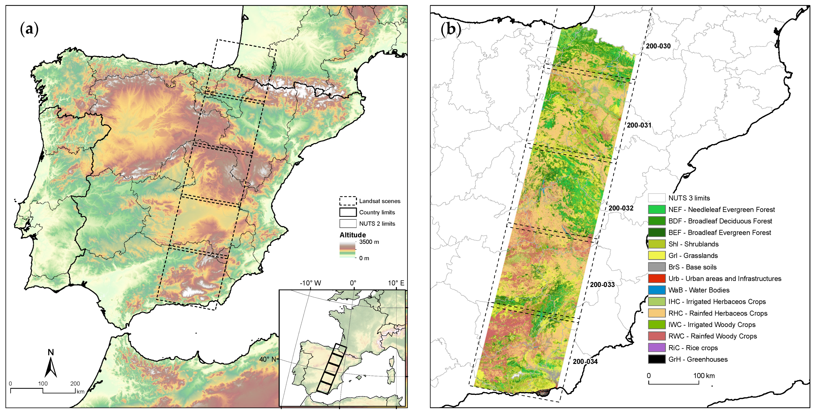
2.1. Study Area

The study area corresponds to a transect of around 185 km wide and 755 km long crossing north–south of the IP and covering 120,190 km² (Figure 1). The transect allows us to study an important bioclimatic gradient where both the Eurosiberian and the Mediterranean biogeographical regions are represented [51]. The south Mediterranean context is characterized by dry conditions where the higher mean annual temperature (19 °C) and the lowest annual rainfall (150 mm) occur, evolving into continental regimes towards the center of the IP. In contrast, more humid and mountainous climatic regimes characterize the North Eurosiberian region, where the lowest mean annual temperatures (2 °C) and the highest annual rainfall (over 2200 mm) are reached. Figure S5 in the Supplementary Materials provide details about the topoclimatic variation along the transect.

The landscape can be divided into two geomorphological scenarios: large depressions drained by the main Iberian rivers (i.e., Ebro, Douro, Tagus, Guadiana, Guadalquivir, and a set of smaller basins) and bounded by mountain ranges of the alpine geological domain (i.e., the Baetic System, the Iberian System, and the Pyrenees). The extensive valleys are covered by recent quaternary materials favorable for agriculture activity.

A high latitudinal gradient characterizes the study ambit regarding climate, topography, and socioeconomic characteristics. Therefore, we subdivided the study area into bioclimatic regions (BRs) (Figure S1) to analyze the NF in local climatic detail. The averaged mean temperature surfaces comprising the 1987–2017 period and the BRs formulation [51] were used to subdivide the transect according to its climatic characteristics. A general overview of BRs is detailed in Figure S4. As will be shown later in the ‘results’ section, regions 1, 4, and 7 (in P1) will not be analyzed as the remaining forest surface was not representative for robust modeling (Figure S6a).

The Spanish National Forest Inventory (NFI 2, 1986–1995 and NFI 3, 1997–2007) was used to identify the predominant forest species in each BR to better understand the forest composition in each region, which is detailed in

Table 1. Main forest species in BRs surveyed in the transect. BR numbers are related to other figures in the text.

Biogeographical Region		Bioclimatic Region (BR)	Main Forest Species 1
Eurosiberian	(1)	Alpine	-
		Subalpine	Pinus uncinata, P. sylvestris (NEF)
	(2)	Montane	Fagus sylvatica (BDF), P. sylvestris (NEF), Quercus pubescens (BDF), P. nigra (NEF), Q. pyrenaica (BDF), Q. petraea (BDF).
	(3)	Coline	P. radiata (NEF), Q. robur (BDF), F. sylvatica (BDF), Q. rubra (BDF), Castanea sativa (BDF).
Mediterranean	(4)	Cryoromediterranean	-
		Oromediterranean	P. uncinata, P. sylvestris (NEF)
	(5)	Supramediterranean	Q. ilex (BEF), P. nigra, P. sylvestris, P. pinaster (NEF) Q. pyrenaica (BDF), Q. faginea (BDF), Juniperus thurifera (NEF), P. halepensis (NEF).
	(6,8)	Mesomediterranean	Q. ilex (BEF); P. halepensis, P. pinaster, P. pinea, P. nigra (NEF).
	(7)	Thermomediterranean	P. halepensis (NEF); Q. ilex and Olea europea (BEF).

¹ The list of species is shorted by dominance in each BR and considering the NFI 3 dataset.

. Thus, the broadleaf evergreen forests (BEsF) and needleleaf evergreen forests (NEFs) were predominant and widely distributed along the transect, while broadleaf deciduous forests (BDFs) dominate in the humid Northern Eurosiberian context.

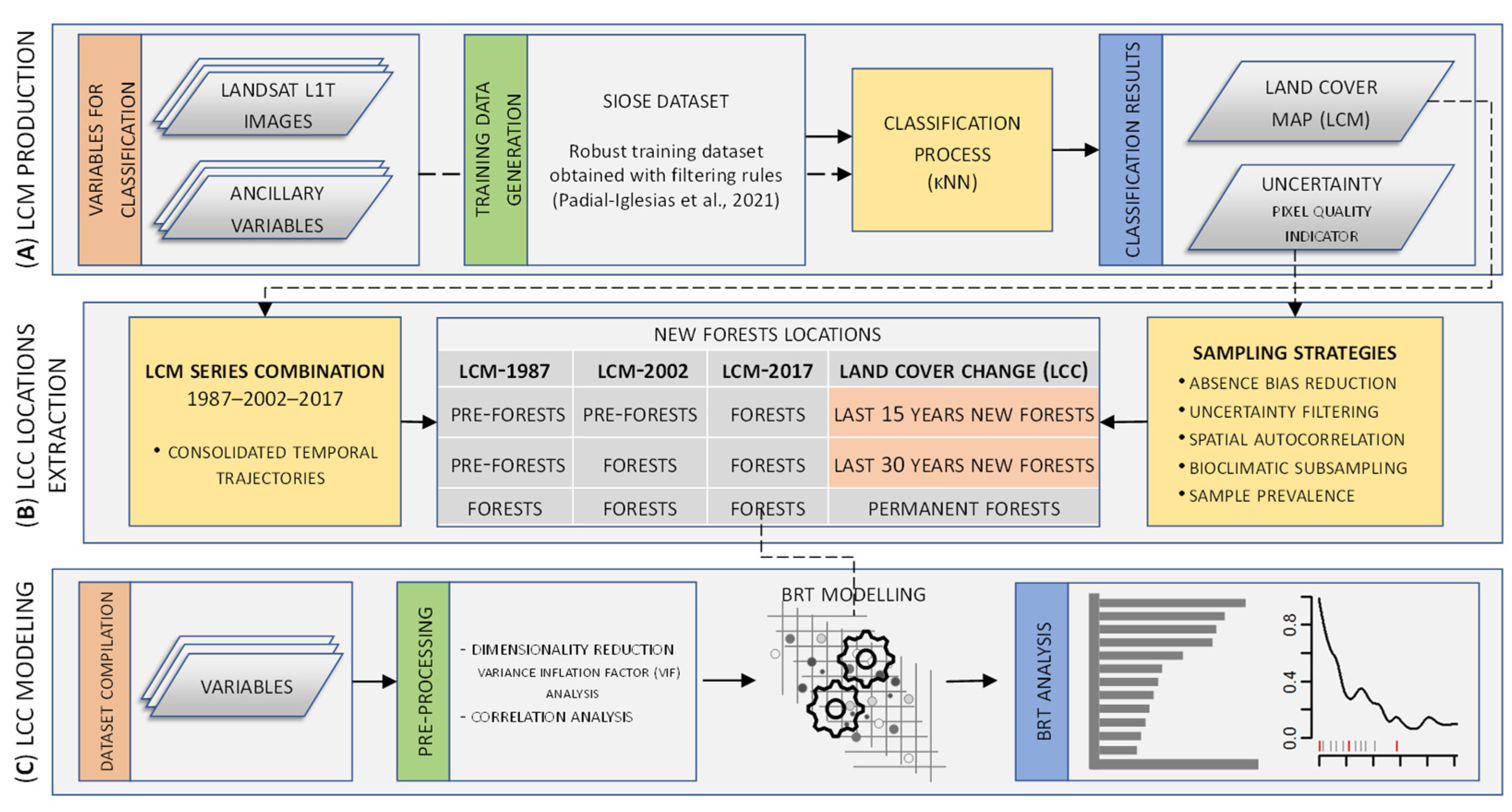
2.2. Methodological Framework

The methodological framework followed in this study is shown in Figure 2, and it is divided into three main stages developed in the following subsections.

2.2.1. Land Cover Map Production

Three LCMs were produced by remote sensing digital classification from 1987 and every 15 years (LCM-1987, LCM-2002, and LCM-2017). LCM have a spatial resolution of 30 m, according to the Landsat imagery series, courtesy of the U.S. Geological Survey (USGS); images were acquired through the website portal (https://earthexplorer.usgs.gov/ (accessed on 16 August 2021)) [52]. The k-nearest neighbor (kNN) classifier was implemented and parallelized in MiraMon GIS and remote sensing software [53]. The classification process followed the methodology detailed in [54,55,56]. In Padial-Iglesias et al. [54], the authors generated accurate ground truth areas using the SIOSE database and filtering rules based on the inner imagery NDVI data to correct inconsistencies in the initial samples by considering inter-annual and intra-annual differences, scale issues, multiple behaviors over time, and labelling misassignments. Furthermore, the authors considered phenologically representative imagery, image preprocessing lines, and auxiliary variables estimation for the classification process. These strategies were crucial for high-quality LCM series achievement, improving the temporal consistency required for LC change analysis.

The MiraMon kNN classifier provides complementary outputs associated with each classified map (e.g., the uncertainty of classified pixels). The uncertainty metric measures the degree to which no class clearly stands out above the others in the assessment of class membership of a pixel. In other words, it expresses complement to one of the degree of commitment to the targeted class relative to the largest possible commitment that can be made. Values range between 0 and 1, where 0 denotes the lowest level of uncertainty and, hence, the most likely accurate thematic pixel assignation. It was used as a filtering strategy to exclude pixels overcoming a level of uncertainty. Its formulation is defined as:

Uncertainty = 1 − (MAX_membership − SUM_membership/N)/(1 − 1/N),

(1)

where the ‘MAX_membership’ argument denotes the maximum set membership value for the pixel, the ‘SUM_membership’ is the total sum of the set membership values for the pixel, and ‘N’ is the total number of the classes considered.

2.2.2. New Forests’ Occurrence Extraction, Sampling on Each BR, and Filtering

In order to model NF locations, explicitly consolidated temporal trajectories were considered. Once a category becomes a forest, it has to remain in later periods to be considered an NF. Similarly, absence locations were those of stable locations in all maps. Furthermore, any presence within fire perimeters polygons was excluded (as explained in Section 2.2.3 and the explanatory variables in the Supplementary Materials) to minimize areas affected by heavy disturbance events along periods.

For text simplicity, this section continues to be explained in a section with the same name in the Supplementary Materials part that gathers the complementary information to the main text. Further references cited in the Section 2.2.2. section that follows in the Supplementary Materials are [4,33,47,48,51,54,57,58,59,60,61,62,63].

2.2.3. Land Cover Change Modeling

The spatio-temporal distribution of forest expansion along the transect and the main drivers involved were analyzed by comparing every two consecutive LCM, i.e., 1987–2002 as the first period (P1) and 2002–2017 as the second period (P2). Dates were defined considering the initials (the mid-1980s) and the most recent Landsat images available at the moment of LC production (2017). The central date (2002) divides the period into two equal 15-year subperiods, coinciding with the auxiliary database date (SIOSE) used to extract training areas [54]. In both periods, each NF dynamic was modeled at the maximum desegregated categorical level (i.e., Grl/Shl to BDF/BEF/NEF and from crop categories to BDF/BEF/NEF), considering a binary presence–absence modeling scheme. The modeling process involved: (1) determining variables that may have potentially impacted the NF occurrence; (2) a dimensionality reduction in predictors, and (3) the model processing itself, developed in the following subsections.

Explanatory Variables

Spatial determinants potentially driving the past NF transitions are listed in

Table 2. Explanatory variables used for modeling forest expansion in the study area. Variables collected at different temporal moments have a value in each period (P1, P2).

Group	Variable	Abbreviation	Units
Topoclimatic	Slope	Slope	Degrees
	General curvature	General_Curv	Dimensionless
	Potential radiation in winter solstice	Pot_Rad_Wint	10 kJ/(m2 × day × µm)
	Averaged annual accumulated rainfall	Ac_Rain	dmm
	Averaged mean annual temperature	Av_Me_Temp	d °C
	Number of drought episodes (DE*)	DE*_S3/6/12	Counts
	Number of humid episodes (HE*)	HE*_S3/6/12	Counts
Distances	Euclidean dist. to forests	Eu_Dist_Forests	Meters
and	Euclidean dist. to hydrography	Eu_Dist_Hyd	Meters
accessibility	Euclidean dist. to protected areas	Eu_Dist_Protect	Meters
	Cost dist. to provincial capitals	Co_Dist_Cap	Meters
	Cost dist. to urban areas	Co_Dist_Urb	Meters
	Cost dist. to main roads	Co_Dist_M_Roads	Meters
	Cost dist. to secondary roads	Co_Dist_S_Roads	Meters
Geology	Lithological substrate	Lithology	Acidic, mixed, alkaline
	Sheet and rill erosion	Soil_Erosion	Mg/(ha × year)
Socioeconomic	Protected areas	Protect_Areas	Protected-Non protected
	Total population	Inhabitants	Inh
	Population density	Pop_Density	inh/km2
	% of population 0–16 years	Pop_0_16y	0–16/inh * 100
	% of population 16–64 years	Pop_16_64y	16–64/inh * 100
	% of population >64 years	Pop_65y	>65/inh * 100
	Ageing index	Ageing_index	>65/(0–16) * 100
	% of agriculture workers	W_Agriculture	W_A/inh * 100
	% of industry workers	W_Industry	W_I/inh * 100
	% of building workers	W_Building	W_B/inh * 100
	% of services workers	W_Services	W_S/inh * 100
	Annual work units	AWU	Work Units
	Number of holdings	Num_Hold	No. of holdings
	Livestock units	LSU	Animals
	Utilized agricultural area	UAA	Hectares

. The selection of biophysical, climatic, distance and accessibility, geology, thematic and socioeconomic determinants was based on a literature review focusing on LC change analysis [4,19,30,57,64,65,66,67,68,69,70]. Selected determinants included variables collected from administrative-level historical statistics and spatially explicit pixel-level data. Details about sources and methods to extract these explanatory variables are given in the Supplementary Materials ‘Explanatory variables’ section. Further references cited in the Section 2.2.3 that follows in the Supplementary Materials are [71,72,73,74,75,76,77,78,79,80,81,82,83].

Collinearity Analysis

The collinearity between predictors was evaluated to exclude variables influenced by other predictors from analysis before modeling, thus reducing model overfitting and time computing. Thus, the level of correlation between predictors was assessed through the variance inflation factor (VIF), considering a VIF threshold of 5 [49]. The process iteratively excludes multicollinearity variables since all the remaining variables had a VIF score below the threshold considered. When two highly correlated variables were detected, the one that depicted a better interpretation behavior in the model and showed a smaller correlation (Pearson’s coefficient) with the other explanatory variables was selected. The process was helpful in reducing dimensionality, especially in socioeconomic, distance-related, and drought-related variables. Subsequently, non-informative zero variance predictors were excluded, and the Pearson correlation coefficients were estimated for the remaining predictors. Lastly, the available presence–absence sample generated was intersected with the predictor variables, resulting in point features with data included in the attribute table.

Data Analysis: Boosted Regression Trees

The LC changes associated with NF transitions were assessed using boosted regression trees (BRTs). BRTs, which coincide with stochastic gradient boosting, are used within a non-parametric regression technique that combine the strengths of decision trees and the boosting ensemble technique [84]. BRTs do not assume any data distribution a priori, which facilitates multiple interactive variables. They also help to identify relevant determinants and their interactions, characterizing their partial dependence. BRTs are currently used in many fields, including remote sensing [33,47], LULC change analysis [46], ecology [4,49,85], hydrogeology [86,87], or marine spatial management [88]. Boosting is sequential, which means that new trees are additively included in a stagewise process and fitted to the residuals of the previous tree [89].

Model Fitting and Parametrization

We applied BRT [84] using the ‘gbm()’ function [48,90] available in the ‘caret’ package [91] in R software [92]. The BRT outputs essentially depend on the settings of four main hyperparameters: the ‘tree complexity’, which is the number of branches or splits for fitting each regression tree; the ‘number of trees’, which defines the number of models composing the final ensemble; the ‘shrinkage’, which is a regularization parameter that controls the model’s influence within the ensemble [89]; and the ‘minimum observations in node’, which define the minimum number of training samples in a node to commence splitting, providing, together with interaction depth, more control on the complexity of the weak learners. Furthermore, the ‘gbm()’ function has two additional parameters: the ‘distribution’ parameter, which defines the loss function, and was set as Bernoulli for binary response variables; and the ‘bag fraction’, which determines the fraction of the observations in a randomly selected training set to fit each weak learner (0.5 for stochastic gradient boosting) [84,89].

We assessed model sensitivity by testing all the combinations of tree complexity levels with the number of trees, the shrinkage, and the minimum number of node observations. A 10-fold cross-validation procedure for each parameter combination determined the optimal configuration to derive the final model. A test subset was used to evaluate the final model performance. The area under the receiver operating curve (AUC) and the accuracy rate measured the model performance [93,94,95,96].

A modeling strategy was performed to extract the five most important drivers (based on the ‘relative importance’) involved in NF dynamics. It was based on three steps. In the first step, an initial model is generated considering the whole set of variables, providing an overall perspective of the most important drivers. The second step gave a new model, considering all predictors but excluding the most important one in the first model. Thus, the repercussion of the first model’s main determinant is excluded, allowing other predictors and their relationships to be evaluated, an exclusion of rising necessity the more significant the variable’s relative importance. Lastly, a final model combines the most important variable of the first model and the four most important of the second one.

The reliability of the final models’ results was evaluated for each NF dynamic. The aim was to corroborate the consistency in the results. We randomly partitioned the available sample into three independent subsets to achieve this sensitivity analysis. Each subset served to derive a training and test subsample used for modeling. The AUC score was used to evaluate model performance, the drivers’ relative importance score, and their partial dependence plots pattern. The results reported similar model performance and main drivers’ relative importance values, as well as PDPs (detailed in the next section) with similar patterns within the five most significant predictors. However, the order of drivers and PDP patterns varied when the subsample size was limited (i.e., <200 points). The results reported consistency and confident interpretations derived from them when the sample size exceeded the minimum estimated sample size.

Model Inference

The BRT technique provides tools for exploring the relationships between explanatory and response variables, estimating the ‘relative importance’ (RI) of the predictors in the model [84,97]. The RI measures the number of times a variable is selected for splitting, weighted by the squared improvement of each split in the model, and averaged over all trees [97]. It is subsequently scaled from 1 to 100 to express the individual contributions as percentages. The RI was calculated for all of the variables in the evaluated models.

To display the results, we estimated the partial dependencies that describe the relationships between the response variable and one explanatory variable while accounting for the average effect of the other predictors [84,97]. This calculus derived partial dependence plots (PDPs) that depict the relationship between the response variable in the space of the predictor and specify the suitable conditions for the LC transition. For each NF dynamic and analysis period model, the five final selected variables were considered to evaluate their importance across time and space (BRs), in addition to their PDPs for pattern interpretation.

As a complement to this, to provide a global perspective of the main drivers involved in each NF dynamics, their predictors’ RI values were aggregated (the sum of the existing individual RI values of a predictor along the BRs), weighted by a factor, and finally scaled from 0 to 100. The factor was estimated as the number of times that a predictor was selected in different BRs divided by the maximum number of BRs where the LC dynamic was modeled; then, it was scaled between [0.5,1] (not between 0 and 1) to avoid a harsh penalization of those predictors selected just in a few BRs.

3. Results

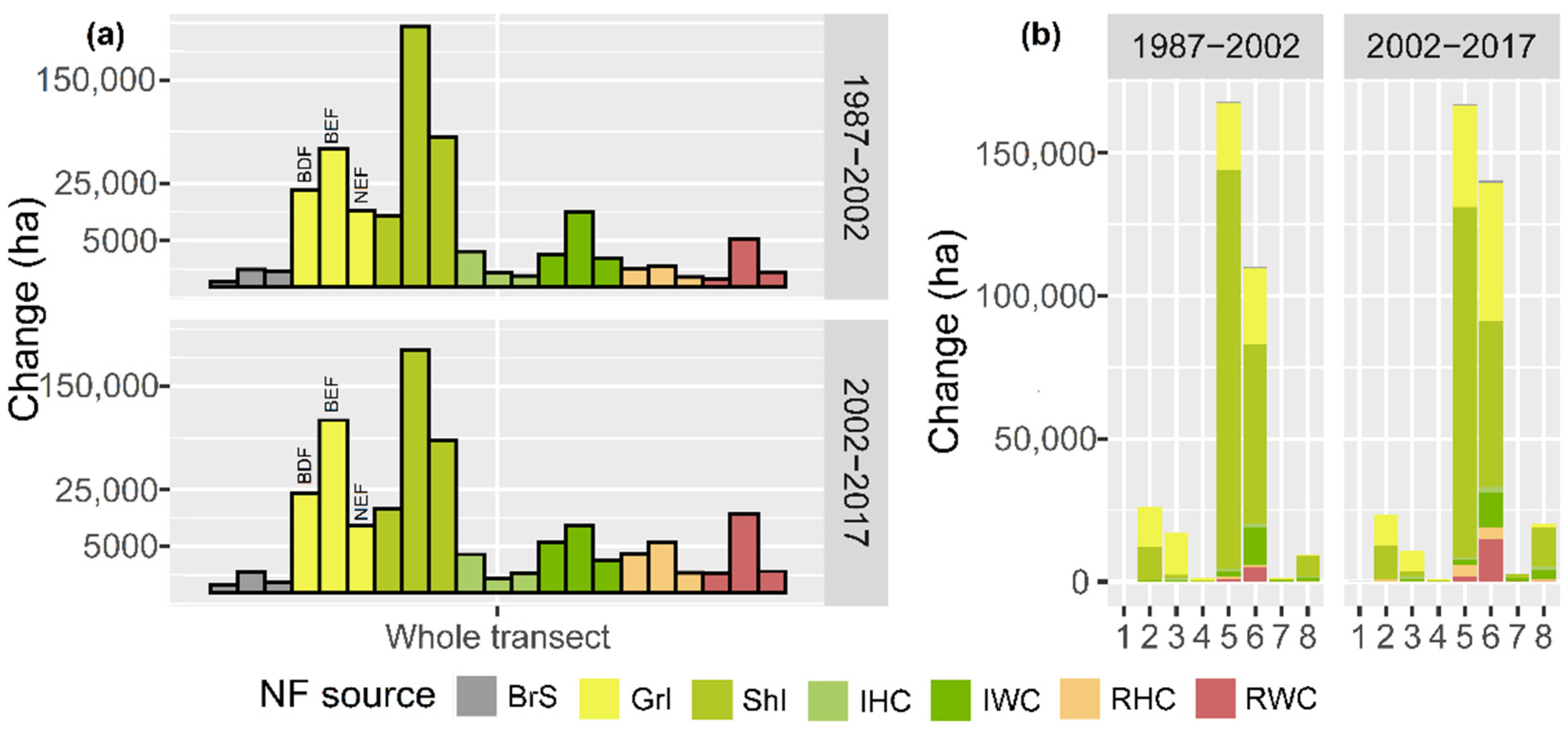
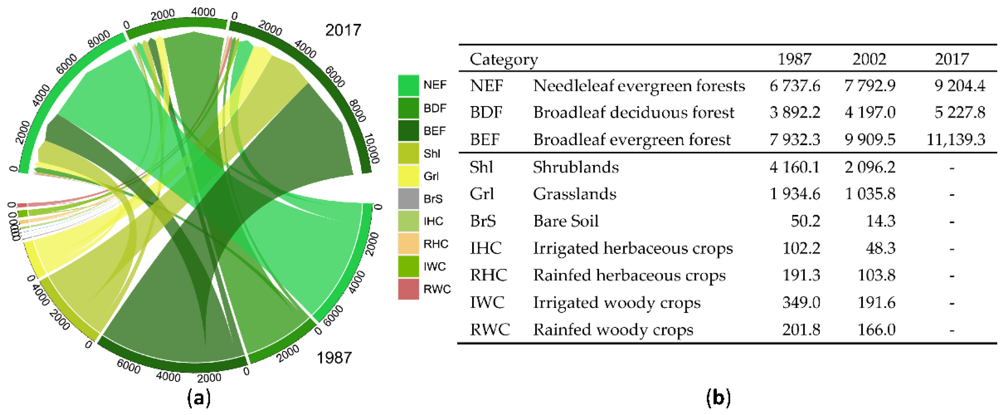
3.1. New Forests Occurrence over the Last Thirty Years

Evaluating all forest land cover trajectories showed that forest expansion exceeds deforestation in extension, implying a positive net forest gain. In the whole transect, forests have increased in the last thirty years mainly at the expense of decreasing shrublands (e.g., 4160.1 km² between 1987 and 2017) and grasslands (e.g., 1934.6 km² between 1987 and 2017) and secondarily croplands (e.g., 349.0 km² of IWC between 1987 and 2017), as detailed in Figure 3. Furthermore, disaggregated details by BRs are shown in Figure S6 in the Supplementary Materials.

Numerically, NF occurrence affected 701,156 ha in the transect (334,031 ha during the first period and 367,125 ha in the second). As seen in Figure 4, the two primary source categories converted into NF areas were related to natural/semi-natural categories (shrublands and grasslands) and cropland abandonment (irrigated/rainfed herbaceous and woody crops) processes.

According to

Table 3. New forest dynamics in absolute and relative values. The source categories’ transitioning area (all figures in ha) towards the target NF group categories (in the upper part of the table) is detailed and disaggregated by the finally modeled BRs and analysis period (P1, P2). In the lower part of the table, figures related to all forests are given to provide final relative figures.

Bio.Region	BR.2		BR.3		BR.5		BR.6		BR.7	BR.8
Target Cat.	P1	P2	P1	P2	P1	P2	P1	P2	P2	P1	P2
NEF	4856.6	4488.8	7933.3	6425.6	31,413.3	24,529.0	18,379.1	20,186.6	1247.8	5743.6	13,973.4
BDF	11,924.0	12,806.6	8128.4	4250.1	15,163.6	25,039.0	3089.3	6451.8	1229.9	1742.3	4817.6
BEF	9434.1	6220.0	1333.9	314.4	121,223.1	117,453.6	88,802.9	114,093.5	323.9	2049.7	2157.9
Abs. Δ NF 1	26,214.7	23,515.4	17,395.6	10,990.1	167,800.0	167,021.6	110,271.3	140,731.9	2801.6	9535.6	20,948.9
Source cat.	↑	↑	↑	↑	↑	↑	↑	↑	↑	↑	↑
Shl	11,969.0	11,773.8	1035.2	1715.7	139,591.7	122,779.5	62,408.0	57,933.2	1042.4	7069.1	13,814.9
Grl	13,860.7	10,759.6	14,732.6	7196.9	23,158.9	35,400.5	26,647.5	48,429.4	143.6	400.7	1086.5
BrS	1.4	3.7	9.8	6.8	594.7	418.6	691.5	897.7	44.2	10.0	24.8
IHC	96.3	47.3	974.7	810.2	770.2	739.8	1347.5	1881.2	54.9	402.5	1294.9
RHC	129.0	690.0	5.5	235.5	871.1	4468.6	693.6	4054.6	18.9	190.4	906.6
IWC	87.9	118.4	474.4	775.4	2020.4	1578.8	13,322.3	12,447.4	1288.2	1202.1	2946.9
RWC	-	0.1	-	0.7	748.7	1551.2	5084.0	14,748.0	147.8	18.2	151.9
Others	70.5	122.5	163.4	248.9	44.4	84.6	76.9	340.3	61.6	242.6	722.4
All forests	388,843.3	375,619.7	89,993.1	92,705.1	1,154,511.0	1,269,076.1	591,780.2	646,504.6	5261.0	58,641.8	57,578.7
NEF	97,215.0	108,544.5	41,852.3	48,364.0	439,790.3	465,941.1	173,548.1	169,650.5	3424.0	43,307.5	39,989.2
BDF	219,789.8	202,775.8	31,018.7	33,119.4	188,810.0	181,902.2	31,272.1	24,467.9	412.9	6108.2	6777.3
BEF	71,838.5	64,299.4	17,122.1	11,221.7	525,910.7	621,232.8	386,960.0	452,386.2	1424.1	9226.1	10,812.2
Shl	78,474.5	68,619.4	5341.4	11,045.0	1,011,593.4	908,174.3	458,904.8	446,259.5	33,579.5	242,900.8	271,144.4
Grl	77,531.0	100,007.2	43,718.1	37,472.8	657,331.5	629,819.3	907,027.6	813,254.9	86,335.2	103,983.7	131,507.4
Brs	988.1	847.5	122.1	169.8	53,807.0	54,331.7	135,633.7	130,237.9	38,382.1	53,041.3	49,668.7
IHC	5871.7	1092.4	14,494.5	8412.7	11,197.8	8053.4	165,911.8	104,488.2	7209.4	127,504.4	108,455.7
RHC	49,705.1	53,484.9	202.4	3787.7	793,903.2	816,432.4	1,878,760.7	1,995,948.0	19,286.3	598,332.8	552,903.8
IWC	1054.2	1646.1	7911.3	7514.0	8755.8	7762.4	271,217.7	246,390.4	32,907.6	88,430.6	100,804.7
RWC	25.3	50.2	0.5	4.7	40,612.4	37,109.3	1,202,153.8	1,217,517.8	142,547.0	110,433.6	100,577.1
Others	1808.7	2934.3	2915.1	3586.9	7206.5	8159.9	35,334.7	46,123.4	37,645.0	28,340.7	38,969.1
Rel. Δ NF 2	6.7%	6.3%	19.3%	11.9%	14.5%	13.2%	18.6%	21.8%	53.3%	16.3%	36.4%

“Others“ includes categories (Urb, WaB, RiC, and Grh) with lower representativeness in NF transitions. ¹ represents the NF absolute increase; ² the relative increase regarding the total forested area (All forests) disaggregated by forest group, and the rest of categories for each BR and period. The main NF dynamics in absolute and relative terms are highlighted in red.

, the NF spatial distribution varied according to BRs, but in general terms, grasslands dominated over shrublands as land donors in the Eurosiberian and the mountainous Mediterranean regions, while the opposite occurred in the Mediterranean area. Crop categories dominated in the Mediterranean, especially in the Mesomediterranean BR. Broadleaf evergreen forests were the principal target forest category (66.3% of NF appearances), and they were mostly concentrated in the Supramediterranean and Southern Mesomediterranean regions. They are followed by needleleaf evergreen forests (20.2%) occupying a wide variability of conditions (from the upper mountain to the driest BRs) and by broadleaf deciduous forests (13.5%) principally located in the Montane and Coline. In absolute terms, the Supramediterranean and Southern Mesomediterranean BRs concentrated afforested areas (47.8% and 35.8%, respectively) due to their extension and geomorphological variability. However, the highest relative afforestation rates were observed in the Thermomediterranean and Northern Mesomediterranean regions.

On the other hand, afforestation was similar in both studied time periods but slightly higher during the second. The afforestation area was higher in the first period in the Montane, Coline, and Supramediterranean regions, and in the second period in the Mesomediterranean (Northern and Southern) and Thermomediterranean regions.

The results were derived from the LCMs, obtained with an overall accuracy—weighted by the ground truth area considering only classified pixels—of 97.2%, 92.2%, and 96.9% at each reference date (1987, 2002, and 2017). The average user and producer accuracy of the natural categories (forest categories, shrublands, and grasslands) were 91.2% and 91.4%, respectively, while the same indicators were 94.8% and 94.3% for crop categories. The confusion matrices of the LCMs and the imagery series considered are detailed in Tables S1–S4 in the Supplementary Materials.

3.2. Model Validation

Table 4. Aggregated, weighted, and scaled relative importance values are detailed for each predictor, source category, and new forests’ target category. The “Irrigated” label groups are IHC and IWC, while “Rainfed” groups are RHC and RWC categories.

Target Forest Categories →	BDF								BEF								NEF
Source Categories →	Rainfed		Irrigated		Grasslands		Shrublands		Rainfed		Irrigated		Grasslands		Shrublands		Rainfed		Irrigated		Grasslands		Shrublands
Periods → Variable ↓	P1	P2	P1	P2	P1	P2	P1	P2	P1	P2	P1	P2	P1	P2	P1	P2	P1	P2	P1	P2	P1	P2	P1	P2
Slope	-	-	5.9	6.9	7.9	7.2	-	-	9.7	5.3	-	18.1	8.3	3.3	9.0	2.4	-	-	-	-	5.5	14.2	4.5	11.9
General Curvature	-	1.0	4.3	5.2	-	-	-	-	-	-	-	-	-	-	-	-	-	-	-	-	-	-	-	-
Pot_Rad_Wint	-	-	-	1.5	10.7	7.9	2.8	14.6	-	2.5	13.4	-	13.6	2.4	18.9	15.7	-	4.9	-	8.6	7.3	1.0	15.0	3.4
Ac_Rain	21.9	12.0	1.3	2.3	11.2	6.5	28.1	23.7	19.5	14.4	-	-	17.8	19.7	13.5	22.3	-	4.3	16.1	23.0	7.8	12.2	22.0	26.7
Av_Me_Temp	-	4.7	2.5	9.3	14.5	10.1	18.7	31.0	3.9	6.8	20.4	27.3	12.8	11.1	14.5	17.0	-	-	-	-	3.8	15.5	3.9	2.3
DE6_S6	-	-	-	-	-	-	3.3	-	-	-	-	-	-	-	-	-	-	-	-	-	-	-	-	1.7
DE9_S6	-	-	-	-	-	-	-	-	-	-	-	-	-	-	-	-	-	2.2	-	-	-	-	-	-
DE3_S12	-	-	-	-	-	-	-	-	-	1.5	-	-	-	-	-	-	-	-	-	-	-	-	-	-
DE3_S24	-	-	-	-	-	-	-	-	-	-	-	-	-	-	-	-	-	-	-	-	-	-	-	1.1
HE3_S12	-	-	-	-	-	-	-	-	-	-	-	-	-	-	-	-	-	-	-	-	-	-	-	1.2
Co_Dist_M_Roads	-	-	5.3	1.1	1.2	-	-	-	-	-	-	-	-	-	-	-	16.1	3.4	24.2	-	-	-	1.5	-
Co_Dist_S_Roads	-	1.6	2.2	-	-	-	-	-	-	-	16.1	-	-	-	-	1.2	-	4.3	-	2.1	-	-	-	-
Co_Dist_Urb	12.7	5.8	2.2	1.8	2.2	5.2	3.9	3.9	1.8	-	-	-	-	-	5.8	-	-	-	-	-	8.6	-	1.9	-
Co_Dist_Cap	18.7	6.4	6.9	8.7	2.8	12.8	4.8	3.6	-	-	-	-	2.0	27.7	-	12.6	31.5	30.6	-	20.7	8.0	11.4	2.0	9.2
Eu_Dist_Forest	26.0	20.9	18.9	11.8	22.5	10.5	24.1	4.2	35.1	35.7	21.2	20.7	24.3	8.9	30.9	14.0	20.9	20.1	-	3.6	28.6	17.2	30.3	18.5
Eu_Dist_Hyd	20.6	24.7	25.9	21.3	-	5.6	-	3.8	2.0	4.9	-	-	-	3.1	-	-	5.8	-	10.5	-	-	1.9	4.0	-
Soil_Erosion	-	-	1.6	2.9	3.0	1.8	-	-	5.4	4.8	28.9	16.7	4.4	-	-	-	12.3	-	24.4	3.6	-	-	1.5	1.0
Protected_Areas	-	-	-	-	-	-	-	-	-	-	-	-	-	-	-	-	-	-	-	-	0.8	-	-	-
Pop_density	-	-	-	1.0	-	-	-	-	-	2.5	-	17.1	-	-	-	-	-	-	-	-	-	-	-	-
W_Building	-	-	-	-	-	-	-	-	2.3	1.7	-	-	-	-	-	-	-	-	-	-	-	-	-	-
W_Services	-	-	-	-	-	-	-	-	2.2	-	-	-	-	-	-	-	-	-	-	-	-	-	-	-
W_Industry	-	-	-	-	-	-	-	-	-	-	-	-	-	1.9	-	-	-	-	-	-	-	4.4	-	-
Num_Hold	-	4.9	-	-	1.9	2.5	-	-	-	-	-	-	-	2.4	-	-	19.3	-	21.9	3.5	-	-	-	-
LSU	-	-	-	-	-	-	-	-	-	-	-	-	1.9	-	-	-	-	-	13.4	2.7	-	-	-	-
UAA	-	-	-	-	-	-	-	-	1.7	-	-	-	-	-	-	-	-	-	-	-	3.2	3.1	-	-
Num. BRs Grouped	1	4	5	6	4	4	2	2	4	4	1	1	4	3	4	4	1	2	1	3	3	3	4	5
BRs Grouped (distinct)	5	5,6 *,8	3,6 *,8 *	3,6 *,7,8 *	2,3,5,6	2,3,5,6	2,5	2,5	5 *,6 *	5 *,6 *	6	6	2,3,5,6	2,5,6	2,5,6,8	2,5,6,8	6	6,8	6	6,8*	2,5,6	2,5,6	2,5,6,8	2,5,6,7,8

* Values with an asterisk denote BRs appearing twice (for herbaceous and woody crops) in grouped categories.

shows the main drivers’ aggregated, weighted, and scaled RI values detailed for each source category and target forest category. This table includes a total of 77 models (28 for BDF, 25 for BEF, and 24 for NEF new forests groups), considering those dynamics in the BRs providing enough samples for modeling. On average, the accuracy obtained in all models was 0.81 ± 0.06 for all the dynamics evaluated. Models in the first period provided an average accuracy of 0.83 ± 0.05 and slightly lower 0.79 ± 0.05 in the second period, mainly related to the higher variability in the NF locations during this period. Regarding source categories, the average values for natural categories were 0.83 ± 0.06 in the first period and 0.78 ± 0.06 in the second. Crop categories showed slightly higher average accuracy, being 0.84 ± 0.04 in the first period and 0.79 ± 0.07 in the second (Table S7).

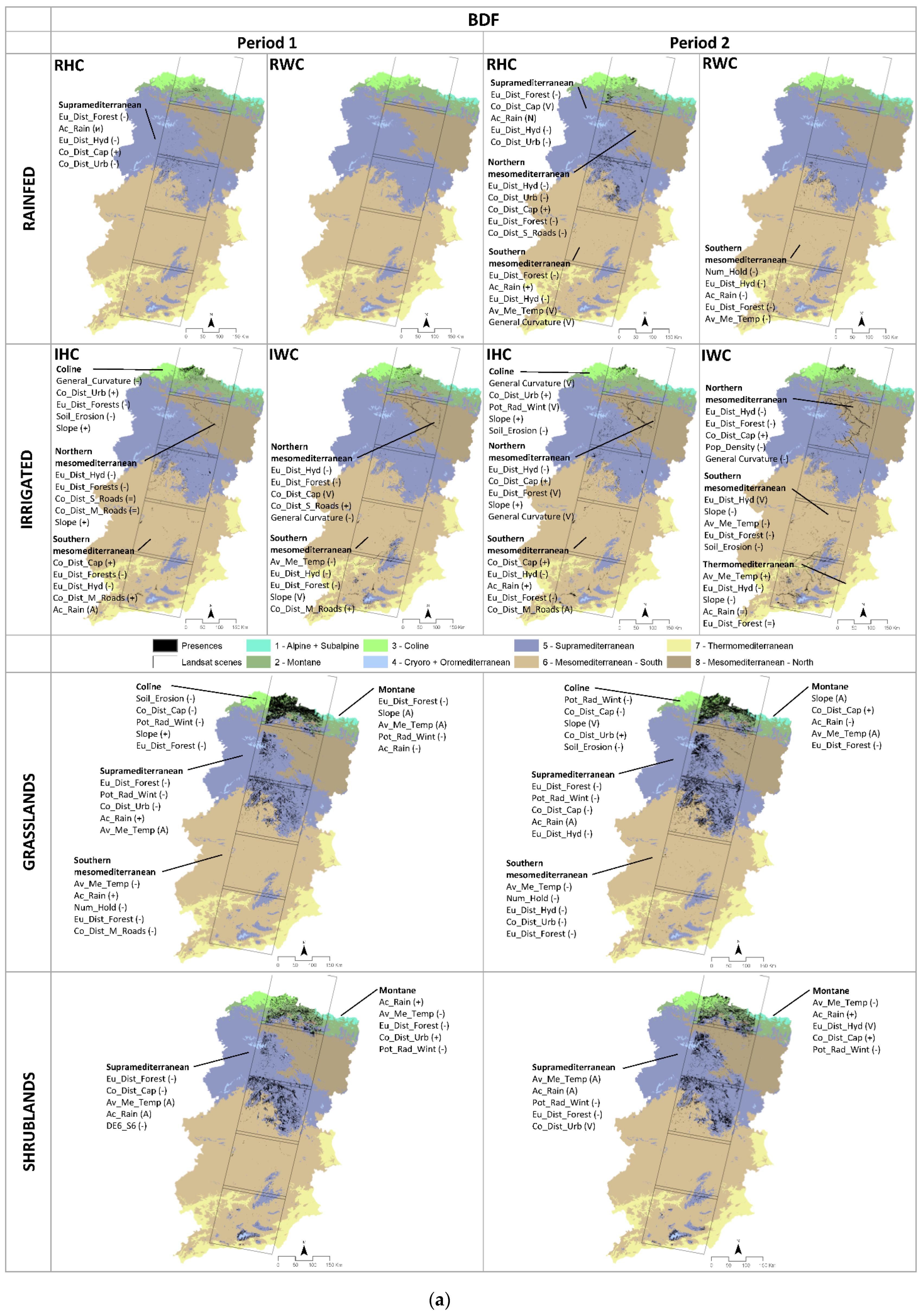
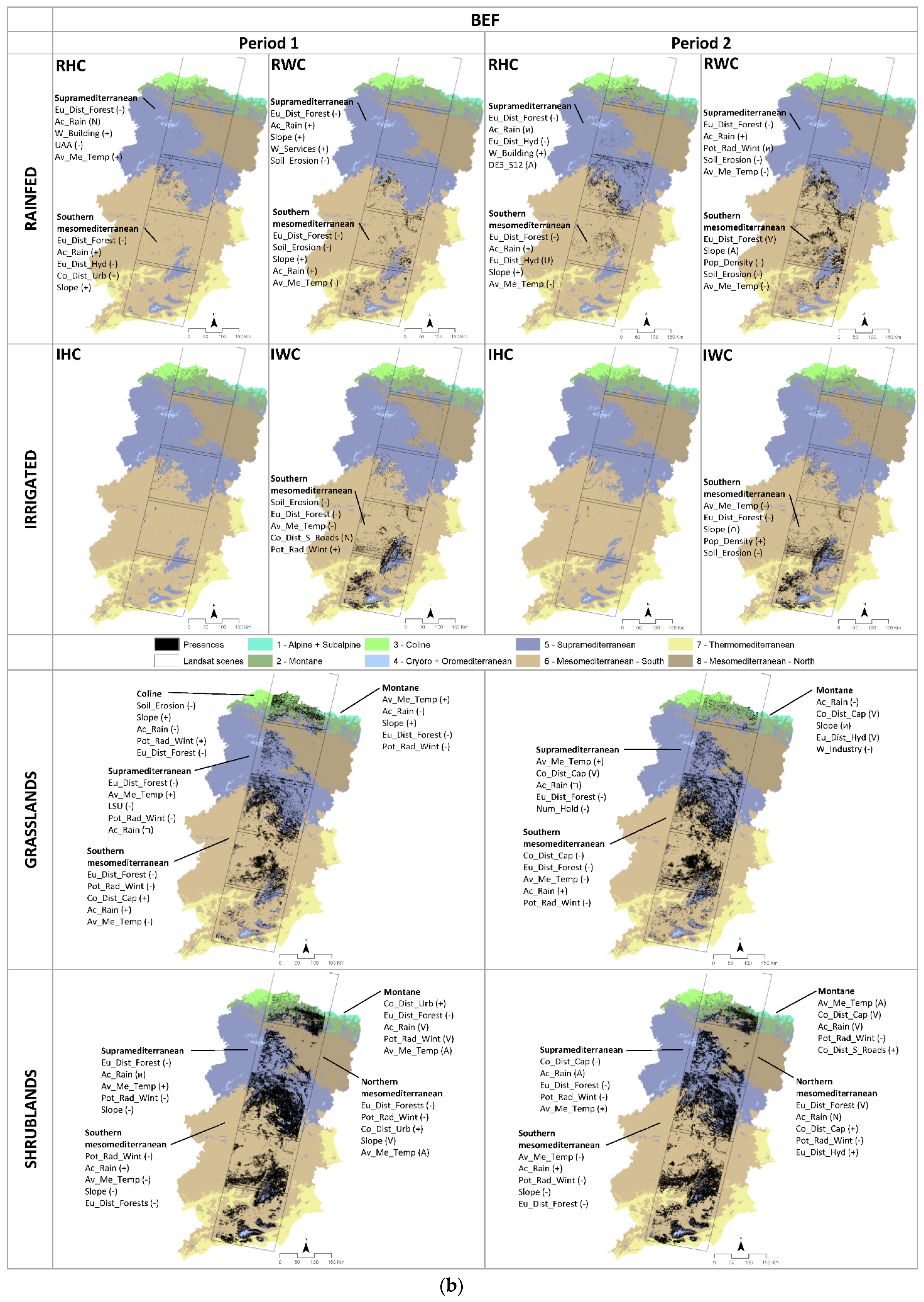
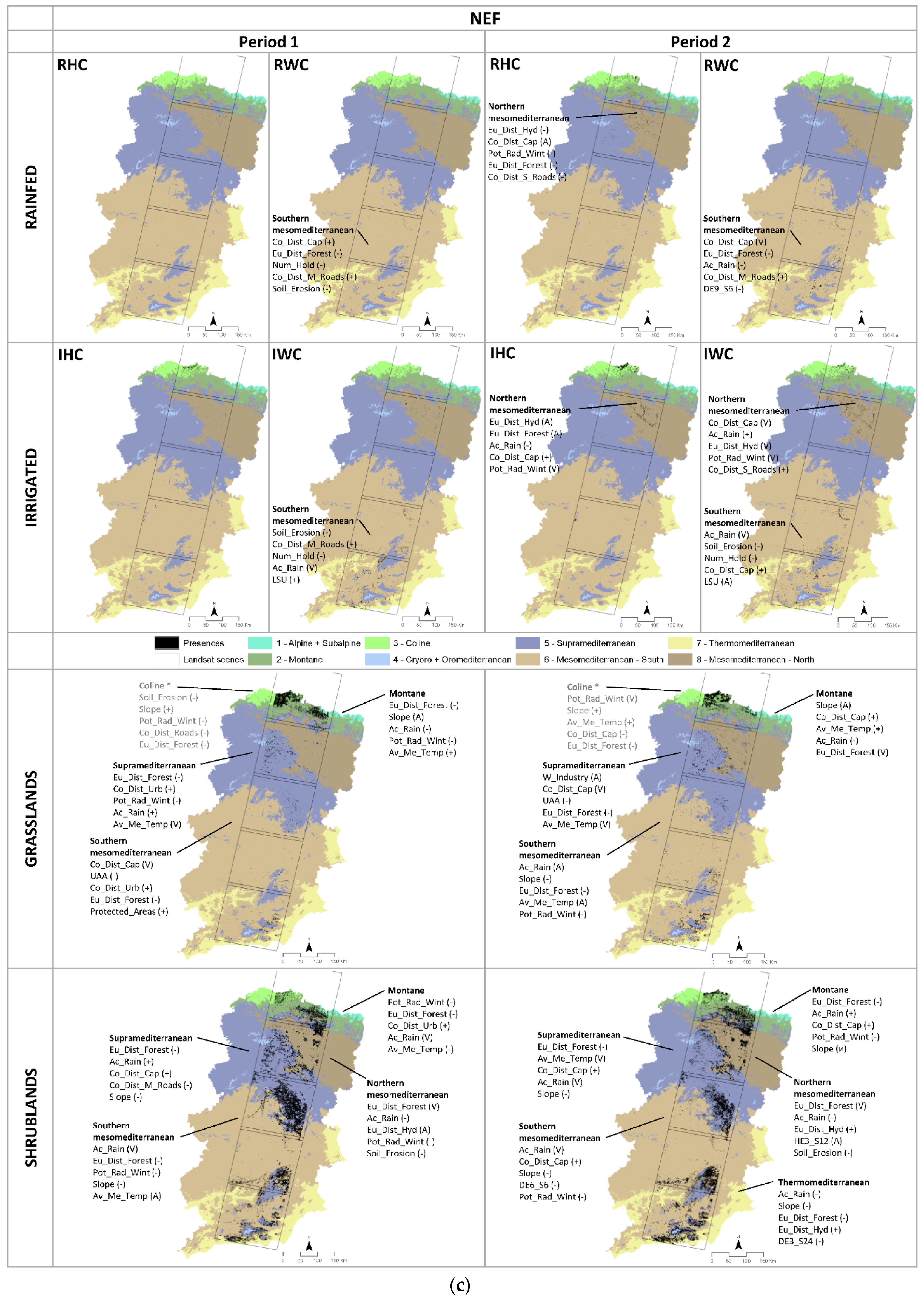
3.3. New Forests’ Main Drivers

The NF driving forces were analyzed by LC source categories (rainfed crop categories, irrigated crops categories, grasslands, and shrublands). From the initial set of variables, twenty-five different variables were among the five main predictors in the models. The maps datailed in Figure 5a–c describe the drivers’ temporal and spatial variation characteristics, detailed by period and BR. Moreover, Table 4 summarizes the driver’s importance for each source category and target forest group. In this section, drivers are listed by their relative importance, accompanied by a symbol (in brackets) denoting the partial dependence main pattern. For instance, the (+grad) means that the transition probability increases with the variable, the (−grad) represents the opposite, and the (≠grad) means that there is not a clear positive or negative tendency. The (A-shape) indicates that the higher suitable conditions occur between two low values, while the (V-shape) denotes two high suitable conditions between a minimum. The (и-shape) depicts relatively suitable conditions in low values that sharply decrease, then increase to a second peak, and finally decrease at larger values. Lastly, the (±grad) is used in the case of different patterns of a driver when aggregating BRs.

A detailed description of the results section is provided in the Supplementary Materials for readers seeking more information, continuing the main text with the discussion of the principal results.

4. Discussion

This study used a sound methodological treatment, which is why we open this section with two subsections discussing its role and contribution. Afterwards, the second subsection continues by examining drivers for the different NF types.

4.1. Land Cover Change Locations Extraction and Sampling Strategies in the Methodological Framework

From a methodological point of view, the training data used during LCM were coherently derived for the whole transect and temporal references, using filtering strategies to enhance their reliability and the quality of their thematic assignment, which also derived in the reliability of the uncertainty threshold applied for the extraction of changing positions [54]. Thus, the filtering rules used to derive ground truth samples provided highly accurate LCM for LC change analysis, together with the uncertainty for each classified pixel. As a result, the maps attained an outstanding performance with an overall accuracy of 95.4% (overall accuracy weighted by the ground truth area considering only classified pixels), providing high-quality information to support the NF analysis.

The accuracy of LCM is frequently influenced by factors such as imagery positional misregistration or wrongly parameterized radiometric correction, deriving in misclassified information. Considering the uncertainty in the dependent variable (NF), it was decisive to use top-performing models. As expected, models’ accuracy increased when pixels with uncertainty over a threshold were eliminated, which is in line with previous research works [57,58].

There are concerns over sampling absence locations and how it could affect the performance of the models, their interpretability, generalization, and transferability. In this sense, different authors show the existence of a bias when obtaining a representative sample of presences–absences in species distribution modeling, proposing various solutions [61,98,99]. Even though this could be an entirely new research line, we considered it necessary to define a sampling strategy to select absences according to the presences available within a spatial buffer, reducing the spatial bias of the absences. Thus, this solution generated a balanced presence–absence sample, assuring their local prevalence.

Finally, the spatial segmentation into BRs was crucial to extract presence–absence locations within similar climatic conditions, enhancing the study’s coherence and avoiding any consideration of absence locations far apart and without spatial relation with the presences in the model.

4.2. Driving Forces Modeling

According to Borda-Niño et al. [66], recent remote-sensing research evaluating forest changes focuses more on deforestation dynamics, and less attention is given to forest increase dynamics. However, understanding the driving forces of NF attending to their source categories is challenging, but decesive to elucidate their contribution to each target forest category, and spatio-temporal patterns. In this research, both local topoclimatic and socioeconomic factors are combined to analyze forestation processes from contrasting LC categories along a representative Eurosiberian and Mediterranean North–South transect.

Studies quite often evaluate the drivers involved in LC dynamics focusing on a specific issue or complex phenomenon to be analyzed, unifying several categories from LC maps into a unique “label”, i.e., forest regrowth, deforestation, and cropland abandonment, which constitutes the phenomenon as a target for analysis in research works [19,21,30,33]. The study also benefited from investigating NF appearance, disaggregated into three forest types, focusing on six main source categories for the sake of understanding the specific drivers involved.

The BRT modeling strategy was based on three steps, and was advantageous in cases where the primary driver in importance in itself explains a large proportion of the variance of the model, i.e., over ~50% of the relative importance. Thus, super dominant drivers, such as the topography, mask the contribution, pattern, and interaction of other predictors with lower explanatory power, which are underrepresented in the resulting models [4,33]. In this research, a solution based on three iterative steps minimized this issue. In the last step, the main driver in the first model and the four most important ones obtained in the second are taken, configuring the final set of drivers that explain the new forest appearance.

In our study, in general terms, topoclimatic and distance drivers were more frequently selected to explain NF dynamics along the BRs than socioeconomics ones, which is a recurrent situation in previous research works [4,7,57]. The lower explanatory power of socioeconomic drivers may be related to their homogeneous spatial distribution into administrative units (municipality, census section). However, we minimized this issue by considering the spatial autocorrelation from the Moran index and a presence–absence balanced sample. Furthermore, statistical analyses are not independent of the spatial configuration or aggregated information scale, leading to severe methodological difficulties such as the modifiable areal unit problem (MAUP) [100,101,102].

4.2.1. Drivers of Forestation from Croplands

Studies of forest expansion associated with cropland abandonment dynamics in mountainous regions have been reported at the European ambit [8,10,103,104,105,106,107,108]. In our results, the appearance of new BDF from crop categories was closely associated with the proximity to rivers, streams, or torrents, where water availability and humidity allows BDF species to grow. Similarly, their expansion is associated with irrigated crops, and is also favored by the proximity to forested areas, producing a fulfilling process between or within the forested patches (small or isolated cultivated areas) or along their edges, where seed dispersal triggers early stages of natural succession [109]. Regarding the spatio-temporal behavior, new BDF from crops mainly appeared in large hydrographic basins close to hydrographic network (Northern and Southern Mesomediterranean BRs) and in the transitions to mountainous areas (Supramediterranean) where croplands are less competitive [110,111,112], affecting specially rainfed crops in our results.

The proximity to pre-existing forests as a driver has been reported in several works [7,30,66,113,114,115], and it has played a crucial role according to our research. Concerning the proximity to the hydrographic network, studies considered and stated it in their results [66,114,115]. This driver affecting riparian vegetation was likely involved in poplar intensification (e.g., Populus nigra L., Populus canadensis L., Populus alba L.) close to rivers and preexisting deciduous species forest plantations. In fact, European initiatives promote the cultivation of poplar tree species because of their sustainability and efficiency (fast-growing and high-carbon sequestration rates) in a context of the need for renewable raw materials and global climate change [116].

For many studies, remoteness has been considered a main driver of NF associated with farmland abandonment [19,30,33,114,115,117]. In our research, the main drivers were the distance to urban settlements, in general, and to provincial capitals, in particular. Thus, the further the distance, the more the likelihood of farmland abandonment. We have also unveiled that croplands further away and less accessible from capital cities were more likely abandoned, which is in line with other works and in other areas [30]. Contrary to initial expectations, the distance to main and secondary roads, as an indicator of remoteness, were not explicative drivers of cropland abandonment, i.e., an outcome similar to other works such as Abadie et al. [115]. In our work, the only exception was in the conversion from crops to NEFs, mainly in the first period when the explanatory power of the distance to main roads was high [33]. One possible explanation could be the high correlation with the distance to provincial capitals, which displays more substantial explanatory power.

Our results showed that the main topoclimatic determinant of crop abandonment to new BDF was precipitation, mainly in the case of rainfed crops with an increasing positive tendency. In some studies, this variable was initially removed due to the correlation with other drivers [30,64], whereas in others, it appeared as the main one [21,66]. Other topoclimatic drivers obtained from our analysis were temperature and slope, with a negative (except for the Thermomediterranean region) and a positive gradient, respectively. These drivers were included in other works [64]. In Spain, Peña-Angulo et al. [118] found rainfall and altitude in the Cameros Viejo region (Iberian System, Spain) as the main factors in deciduous forest appearance from cropland abandoned in mountainous areas. Moreover, Alonso-Sarría et al. [119] found that climatic drivers (precipitation and temperature) predominated over geomorphological drivers in land abandonment in the Murcia region (Spain). These findings align with our results since climatic drivers were more represented and of higher importance in the warmest and driest BRs.

Within the socioeconomic variables, rural depopulation has been associated with the abandonment of agricultural land and subsequent natural succession dynamics, especially in the European mountain areas [8,103,107,112,120]. However, in our results, the role of depopulation dynamics was of low importance and was associated with a lower population density driver. Nevertheless, variables related to the agricultural structure of the holding played an important role in the Southern Mesomediterranean BR. In this context, NFs were favored in areas with a lower number of holdings devoted to rainfed woody crops in the limit with the Supramediterranean region, where the number of holdings is lower compared to lowlands in the middle of the large basins and presumably smaller agriculture holdings due to terrain (slope, area) limitations. In this line, Zglobicki et al. [121] found that holding size can drive land abandonment in eastern Poland. Nevertheless, in general terms, population and the agricultural structure driving forces were scarcely represented in our model results.

In the case of new BEF from crop abandonment processes, the proximity to previously forested areas remained as the main driver in all the BRs involved (mainly located in the south of the transect), and the distance to the hydrographic network disappeared as a consequence of much lower water requirements of evergreen forest species. Regarding the spatio-temporal behavior, new BEFs from crops mainly appeared in Supramediterranean and Southern Mesomediterranean BRs, and especially in the transition between them. Contrary to BDFs and NEFs, distances and accessibility drivers, such as the distance to provincial capitals, urban settlements, and roads, showed scarce importance. Why remoteness is less informative is unclear and will be of interest in future research.

The main topoclimatic driver of new BEFs from crop abandonment was temperature, mainly in the case of abandoned irrigated crops, showing a decreasing negative tendency. Thus, the higher relative importance was associated with the warmest southern BRs. Another driver was precipitation, associated with a positive trend to rainfed crops, especially in the Southern Mesomediterranean region. This was interpreted as a NF in the upper limit of the BR at higher altitudes, where total accumulated precipitation is high. Therefore, water availability and temperature were major drivers in the warmest areas of the transect, which is in line with studies performed in semi-arid regions [119,122]. Lastly, NF appearance was favored by steeper slopes, a pattern also observed in several studies [115,123,124,125].

Soil erosion showed a significant role in irrigated woody crops, with a general negative tendency, meaning that NF occurred in areas showing scarcely erosive processes. According to previous research, the intensity of soil erosion is controlled by the vegetation cover and land uses, which is considered to be more critical than slope and precipitation intensity, even though the low-frequency and high-intensity precipitation extreme events are generally responsible for soil erosion [126,127]. The revegetation process after the land abandonment in mountain areas during the 20th century resulted in a reduction in soil erosion, whereas sheet erosion, piping, or gullying affected abandoned crop fields in semi-arid contexts [128,129]. This driver has been fairly well studied in LC change analysis, such as by Bakker et al. [130,131], where the authors found soil erosion as an important driver of land use changes, for instance, in agricultural de-intensification processes favoring the reduction in erosion and sediment movement.

Compared to BDF, from our results, socioeconomic drivers played a specific role in the Supramediterranean and the Southern Mesomediterranean BRs. NF appearance preferentially occurred in areas with a higher percentage of the population employed in building and service activities, as well as low/high (rainfed/irrigated woody crops) densely populated locations, more prone to be abandoned. Similarly, Vidal-Macua et al. [19] identified crop abandonment in the central Pyrenees in areas with a higher proportion of population employed in the service and building activities, which are job opportunities generally outside the agriculture sector [7]. In the Sierra de Albarracín (Spain), Melendez-Pastor et al. [132] found a clear reduction in the population employed in the primary sector, stability in the secondary, and a significant increase in the tertiary sector related to the promotion of rural tourism.

In the case of new NEFs from crop abandonment processes, the distance to provincial capitals, forests, and secondary roads predominated in all the BRs involved. Moreover, the number of holdings and the livestock units dominated in the southern region, and the distance to the hydrographic network dominated in the northern region. Regarding the spatio-temporal behavior, new NEFs from crops appeared in the Northern and Southern Mesomediterranean BRs, areas characterized by dry conditions, where NEF species (e.g., Pinus halepensis Mill., Pinus pinaster Aiton, Pinus pinea L., and Pinus nigra J.F.Arnold) are better adapted to lower water requirements.

Remoteness played a significant role through the distance to provincial capitals (mainly) and the distance to roads, both with a positive tendency, i.e., a larger distance away from capital cities and roads signalled a higher likelihood of croplands being abandoned, as discussed in other works [30]. The proximity to pre-existing forests showed lower importance than in the case of new BDF and BEF.

The main topoclimatic driver of new NEFs from crop abandonment was precipitation, with irregular (positive and negative) trends along BRs. Thus, in the Southern Mesomediterranean, the V-shape indicates a non-linear pattern related to occurrences in the plain areas (lower precipitation) and the BRs’ upper limit (higher precipitation). Finally, soil erosion played a significant role in the IWC category (similar to new BEF), with a clear negative tendency, meaning that NF was again favored in areas showing scarcely erosive processes. Thus, spontaneous vegetation (meadow, pastures) can promote low erosive situations and act as protection cover in humid conditions.

Compared to BDF and BEF, socioeconomic drivers were significant in the Southern Mesomediterranean BR, where new NEF appearance was more prone in areas with a low number of holdings. This fact is interpreted as the lower availability of agriculture holdings in the upper limit of the BR, far from provincial capitals and main roads. In addition, remoteness and climatic constraints reduce the productivity of the land, increased by uncertainty in the regularity of rainfall, making farmers more likely to make decisions aimed at abandoning land [11,119,122]. Finally, a positive trend related to livestock units has been observed, a totally new contribution up to our knowledge.

4.2.2. Drivers of Forestation from Grasslands

Studies of forest expansion in mountainous regions are numerous, and there are plenty of examples which consider the whole European ambit [10,31,133,134], as well as regional studies in Albania and Romania [33], Colombia [69], Portugal [135], Spain [19,57,132,136], Russia [40], or Slovakia [112].

According to our results, the appearance of new BDF from grasslands was closely related to the proximity to forested areas, in addition to topoclimatic drivers such as temperature, solar radiation and precipitation, and distance drivers (such as the distance to provincial capitals). Regarding the spatio-temporal behavior, new BDFs from grasslands appeared mainly in the more humid mountainous BRs, i.e., Montane, Coline, Supramediterranean, and Southern Mesomediterranean. The proximity to forested areas was the main driver in the Montane and Supramediterranean BRs and secondary in the others, indicating a homogenization and fulfilling process within the forested patches or along their edges, enhanced by seed dispersal triggering the early stages of natural succession [109]. This driver also was considered in other research works [7,30,114,115].

The main topoclimatic driver was temperature, showing high importance and a decreasing negative tendency in the Southern Mesomediterranean region, as well as moderate importance and non-linear (A-shape) tendency in the Supramediterranean and Montane. Furthermore, precipitation appeared with temperature and showed a negative trend in the Montane BR and a positive trend in others. Moreover, a negative tendency in the solar radiation was generally observed, in addition to steeper slopes in the Montane and Coline BRs, which was also observed in previous research [115,123,124,125]. Lower solar radiation rates and humid conditions were also reported by Vidal-Macua et al. [4] for this LC dynamic, and Borda-Niño et al. [66] found the proximity to forests and slope as the main factors which can positively influence forest regrowth. In the Supramediterranean, higher precipitation and lower solar radiation favored the new BDF appearance, which is in line with Diaz-Delgado et al. [137], finding a significant negative correlation between the vegetation recovery (from fire disturbance) and solar radiation and a positive correlation with precipitation. Furthermore, Pérez-Luque et al. [138] analyzed Quercus pyrenaica colonization over abandoned cropland in the Sierra Nevada mountain range (Spain) in the rear edge of their distribution and near mature forest on mainly southern-oriented hillsides.

Remoteness has been considered a primary driver of NF associated with farmland abandonment and subsequent natural succession. In our results, remoteness indicators were mainly represented by the distance to provincial capitals, urban settlements, and secondarily main roads. Thus, new BDFs from grasslands were generally more likely at a shorter distance to them in all BRs, except for the Montane region at a higher distance to provincial capitals. Similarly, farmlands located close to provincial capitals were more likely to be abandoned in the Polish Carpathians [7], a process explained by new job opportunities outside of the agricultural sector or even by the pressure to change agrarian land use in the suburban areas for residential promotion [139]. Similarly, other studies found forest and shrubland regeneration near roads and urban sectors, where more off-farm opportunities in the vicinity of roads can occur [114,140].

The structure of agricultural holdings played a secondary role in the Southern Mesomediterranean BR. In this context, NFs were favored in areas with a lower number of holdings on the limit with the Supramediterranean region, which coincided with the patterns observed in new BDF from rainfed woody crops. The similarity in patterns and spatial context suggest that crop fields abandoned at different ages coexist in this area, as grasslands signal the decay of tillage works and the initial natural succession process.

The appearance of new BEFs from grasslands was associated with topoclimatic drivers, such as precipitation, temperature, and solar radiation, as well as distance drivers, such as the proximity to forested areas and the distance to provincial capitals. Regarding the spatio-temporal behavior, new BEFs from grasslands appeared with lower density in the Montane and Coline and with more intensity in the Supramediterranean and Southern Mesomediterranean BRs, as was initially expected compared to BDF, due to the adaptability of broadleaf evergreen species (Quercus ilex sensu lato), through their high water-use efficiency, to drier conditions.

The main topoclimatic driving forces were precipitation, temperature, and solar radiation, showing different importance and patterns. For example, new BEFs from grasslands in the Montane region were favored by higher temperature, lower precipitation, and solar radiation on steep slopes, which denote NFs establishing at lower altitudes on steep hillsides with lower humidity conditions. Similarly, these patterns were observed in the Coline BR but with a positive solar radiation tendency, where water availability is less restricted. However, temperature (together with precipitation) showed opposite patterns in the Supramediterranean and Southern Mesomediterranean BRs, with positive and negative tendencies, respectively.

In our results, remoteness was represented by the distance to provincial capitals. Thus, new BEFs from grasslands were more likely to be closer to and further from the main provincial capitals, in the mountainous regions, i.e., the Montane and Supramediterranean. This double pattern can be associated with the pressure of change agrarian land use close to main urban areas [139] and related to the declining agricultural activities and the land abandonment of less productive and remote land fields [110,141]. Furthermore, in the Southern Mesomediterranean, two temporal patterns were observed (Figure S7b3). In the first period, the new BEFs from grasslands predominantly were further from provincial capitals, while in the second period, they were closer to them. This can be interpreted as a first wave of land abandonment process mainly in the high lands, and a second wave in lowlands closer to main capitals, which coincided with the temporal pattern of temperature, showing an increase in the mean temperature (lower altitude) in the second period.

Indeed, regarding the structure of agricultural holdings, a negative tendency in the livestock units (and the number of holdings) was observed in the Supramediterranean BR. This pattern is in line with the de-intensification of agricultural activities (livestock grazing reduction and cropland abandonment) and the forest expansion process in mountainous areas identified in previous research works [12,141,142].

Grasslands’ successional dynamics towards NEFs showed an intensive temporal dynamism. New NEFs from grasslands were related to proximity to forested areas, as well as topoclimatic drivers (such as precipitation, slope, and temperature) and distance drivers (such as the distance to provincial capitals). Most of the occurrences were in the Montane, Supramediterranean, and the Southern Mesomediterranean BRs, with the last two being the most dynamic between periods. Similarly to BDFs and BEFs, the proximity to pre-existing forests was significant for new NEF from grasslands, especially in the Montane and Supramediterranean, and secondary in the Southern Mesomediterranean BRs.

Regarding proximity to forests, previous studies in the central Pyrenees (Spain) found that the tree line remained almost static, while the forest patch density increased in a context of climate warming and LC change [143,144]. Thus, areas near forests and declining grazing pressure have promoted natural succession dynamics in the central Pyrenees. In the Urbión Mountains (Iberian System, Spain), Sanjuán et al. [142] analyzed a subalpine belt affected by intense deforestation, leading pastures for grazing since the middle of the past century. Subsequently, declining livestock pressure and the depopulation process resulted in the encroachment of shrublands and the expansion of conifer forests at the expense of grasslands and shrublands.

Concerning topoclimatic drivers, slope steepness and lower solar radiation enhanced the likelihood of conversion from grasslands to forests, in line with previous research in mountainous areas [113]. Furthermore, precipitation showed a negative tendency in the Montane and a positive tendency in the Supramediterranean BR, suggesting lower humidity requirements for new NEF to be established in the Montane but higher humidity requirements in the Supramediterranean and Southern Mesomediterranean regions according to the BR’s range of values. Remoteness in the form of the distance to urban settlements and the distance to provincial capitals showed a generally positive trend, in line with the main drivers of the extensification dynamics found by Pazúr et al. [30].

Furthermore, our results showed that drivers in the Supramediterranean BR evolved towards socioeconomic drivers during the second period, with laboring in industry, utilized agricultural area, and distance to provincial capitals being the main drivers. This pattern suggested a lower contribution of the distance to forests, distance to urban settlements, and solar radiation during the second period, allowing socioeconomic drivers to appear. In contrast, the Southern Mesomediterranean region was related to the distances and socioeconomic drivers, evolving during the second period to topoclimatic driving forces. This was interpreted as the larger contribution of remoteness and socioeconomic drivers in the highlands during the first period and topoclimatic in the lowlands in the second.

4.2.3. Drivers of Forestation from Shrublands

Studies of forest expansion associated with land abandonment and natural succession analyzing forest encroachment are numerous, but are also specifically limited for shrublands [4,41,114,124,142,145,146].

According to our results, the appearance of new BDFs from shrublands was related to topoclimatic drivers (such as precipitation, temperature, and solar radiation) and distance drivers (such as the distance to forests and distance to provincial capitals). Regarding the spatio-temporal behavior, new BDFs from shrublands mainly appeared in the mountainous BRs, i.e., the Montane and Supramediterranean.

The main topoclimatic drivers were precipitation and temperature, and secondarily solar radiation. In the Montane BR, topoclimatic drivers were the main drivers; precipitation showed a positive tendency, while a negative tendency was observed for temperature and solar radiation. This pattern suggests that new BDFs from shrublands was favored by high precipitation, low radiation, and temperature (higher altitude). This binomial of low temperature and low radiation was in line with higher altitude (lower temperature) and lower radiation, as found by Vidal-Macua et al. [4] in a similar geographic context. Furthermore, these patterns were maintained in the second period, suggesting similarities in climatic drivers over time. Meanwhile, in the Supramediterranean BR, temperature and precipitation followed a non-linear tendency (A-shape) in both periods, suggesting that the most likely conditions are maximized on shady hillsides with temperature and precipitation constraints. Complementarily, the occurrence of medium-term droughts (6-month SPEI timescale) of at least six consecutive months was negatively related in the first period, suggesting a lower tolerance of BDF species to drought.

The proximity to forested areas was the main driver in the Supramediterranean BR and the secondary driver in the Montane during the first period, indicating the homogenization and fulfilling process in forest patches and along their edges, even further during the second period. This driver was considered in previous research works [7,30,114,115].

Remoteness was represented by the distance to provincial capitals and to urban settlements, generally denoting a positive tendency in the Montane BR. However, the tendency was negative in the Supramediterranean, indicating more likely conditions in areas near urbanized areas, which coincide with research works focusing on the land abandonment process [7,41,43]. Furthermore, these patterns were similar to those observed in the case of BDF from grasslands.

The appearance of new BEF from shrublands was associated with distance drivers, such as the distance to forests and to provincial capitals, in addition to topoclimatic factors, such as precipitation, solar radiation, and temperature. Regarding the spatio-temporal behavior, new BEFs from shrublands appeared more densely in the Montane, Supramediterranean, and Southern Mesomediterranean BRs, and with lower density in the Northern Mesomediterranean.

The distance to forests was the main driver in all BRs except in the Southern Mesomediterranean, with topoclimatic drivers predominating. It showed a negative trend in all cases. A general decrease in the relative importance in the second period suggests that the forest completion and fulfilling process observed in the first period continued at a greater distance in the second. Woody encroachment due to the expansion of forests and shrublands (at the expense of grasslands) has been reported in mountain areas, confirming densification and expansion through the tree line [147,148,149].

Remoteness was represented by the distance to urban settlements in the first period and by the distance to provincial capitals in the second. In the Montane and Northern Mesomediterranean BRs, the most suitable conditions occurred far from urban areas and near forested areas in both periods. However, the opposite pattern was found in Palmero et al. [105] for forest expansion in temperate and Mediterranean regions on a European scale. Moreover, a negative trend was observed in the Supramediterranean region for the distance to provincial capitals, which agrees with previous research [114]. Furthermore, NFs in the proximity to provincial capitals can be explained by the increase in new job opportunities outside the agricultural sector or by the pressure to change agrarian land use in the suburban areas for residential promotion in agricultural abandoned areas [139]. Farmland abandonment probability increases when employment redirection to other sectors occurs [8].

The main topoclimatic drivers were precipitation, solar radiation, and temperature with different tendencies in BRs. In the Montane, precipitation followed a positive trend, while temperature and solar radiation were negative. This pattern suggests that new BEF from shrublands was favored by higher precipitation and lower radiation and temperature (higher altitude). Binomial low temperature and low radiation were both in line with higher altitude (lower temperature) and lower radiation, as reported by Vidal-Macua et al. [4] in a similar geographic context. Furthermore, these patterns were maintained in the second period, suggesting similarities in climatic drivers over time. Meanwhile, in the Supramediterranean BR, precipitation and solar radiation followed a negative tendency and a positive one for temperature, suggesting that the most likely conditions are maximized at a lower altitude and on shady hillsides with less water availability, as sclerophyllous forests are adapted to lower water requirements in this region. These patterns are consistent with previous studies analyzing land abandonment processes and natural succession at lower altitudes on north-oriented hillsides [150]. In the Southern Mesomediterranean BRs, temperature and solar radiation followed a negative tendency and positive one for precipitation, which coincides with the drivers’ pattern in the southern Landsat scene spatial context analyzed by Vidal-Macua et al. [4]. It suggests that the most likely conditions occurred at higher altitudes, on shady hillsides with less water availability in the BR, corresponding to areas with lower slope values in the proximity to forested mountainous areas close to the upper BR limit (Supramediterranean).

Shrublands’ successional dynamics towards NEFs were related to the proximity to forested areas, topoclimatic drivers (such as precipitation, solar radiation, and slope), and accessibility drivers (such as the distance to provincial capitals). New NEF occurrences dominated in all BRs except for the Coline. Similarly to BEFs, in the case of new NEFs from shrublands, the proximity to forested areas played a major role, especially in the Montane, Supramediterranean, and Northern Mesomediterranean BRs. This pattern coincides with a homogenization, fulfilment, and expansion of the forested areas. Woody encroachment due to the expansion of forests and shrublands has been reported in mountain areas, confirming densification and expansion through the tree line [147,148,149].

Remoteness was represented by the distance to provincial capitals and urban settlements. The most suitable conditions occurred far from urban areas in both periods in the Montane, Supramediterranean, and Southern Mesomediterranean BRs. However, the opposite pattern of forest expansion was observed on the European scale [105]. On the other hand, the main topoclimatic drivers were precipitation, solar radiation with different tendencies in BRs, and the slope with an overall negative trend.

In Montane areas, precipitation followed a non-linear tendency (a general positive tendency falling at high precipitation values) and a negative trend for solar radiation and temperature. Thus, it suggests that NEFs from shrublands were favored at lower and higher humidity regimes (up to a limit) on shady hillsides at higher altitudes, while NEF species (Pinus sylvestris, P. nigra) are better adapted. These findings agree with Vidal-Macua et al. [4] in the Pyrenean context, where transitions to coniferous forests were favored at higher altitudes (lower temperature) and a lower radiation.

In the Supramediterranean context, precipitation followed a positive tendency, a negative for slope. The results suggest that the higher precipitation rates, the lower slopes, and the absence of solar radiation as a driver promoted new NEF (Pinus nigra, P. sylvestris) in more plain areas at higher altitudes, where the higher precipitation occurs. Melendez-Pastor et al. [132] identified a clear forest regeneration (mainly pine forest) in the Sierra de Albarracín (North Iberian System, Spain), at the expense of mainly shrublands and farming areas for the first period of analysis. Furthermore, Sanjuán et al. [142] found clear patterns of shrublands and clear forests evolving towards dense forests of Pinus sylvestris, in south-facing and stepped slopes in the Urbión Mountains (Iberic System, Spain).

Similarly, in the Southern Mesomediterranean, precipitation followed a non-linear tendency denoting higher likelihood at low/high precipitation values according to dominant species. Indeed, a negative trend in slope and solar radiation, suggesting that new NEF appearances took place in the more xeric (Pinus halepensis) and humid (P. pinaster, P. nigra) context of the BR, was favored by shady conditions. These findings agree with the lower solar radiation and soil moisture dependence in the transition of shrublands to conifers in a similar context of analysis analyzed by Vidal-Macua et al. [4]. Furthermore, medium-term drought occurrences (6-month SPEI timescale) of at least six consecutive months was negatively related to shrubland encroachment to new NEF in the second period, denoting better conifer species plasticity to growth in lower drought conditions.

Lastly, in the Thermomediterranean BR, precipitation and slope followed a negative tendency, together with a negative trend in long-term drought occurrences (24-month SPEI timescale) over at least three consecutive months. Unexpectedly, these results suggest that lower precipitation rates favored new NEF forests on low-sloped hillsides, which, to a certain extent, could promote drought-tolerant conifers species (Pinus halepensis) adapted to arid climatic conditions. This pattern agrees with local studies in the Murcia region, where land abandonment processes and related successional dynamics were negatively associated with precipitation [119]. Therefore, climate factors and water availability, specifically in semiarid regions, determine land productivity (even irrigated plots, depending partly on precipitation) and increase the uncertainty about the rain irregularity [11], affecting cropland and natural vegetation productivity. Moreover, Vidal-Macua et al. [19] found a positive relation between crop abandonment and medium-term droughts occurrences (6-month SPEI timescale) over at least 7–8 months in the central Ebro basin.

4.3. Answers to the Hypotheses

According to our first hypothesis, NFs are mainly associated with successional dynamics, i.e., shrublands and grasslands, and secondarily with crop abandonment processes, i.e., the main sources along the transect. Natural/semi-natural source categories predominate in absolute values along the transect. In relative terms, 17.2% and 7.52% of natural surfaces, in addition to 2.86% and 0.69% of croplands, evolved towards NF in the Eurosiberian and Mediterranean biogeographic regions, respectively. The transect also revealed contrasting driving forces (topoclimatic and socioeconomic) throughout space and time. In the Eurosiberian area, distance to forests was selected in 20.0% of cases, solar radiation in 17.8% and precipitation in 15.6% in the first period, while the distance to provincial capitals was selected in 17.5% of cases and precipitation and slope in 15.0% in the second period. Only on one occasion were socioeconomic drivers selected in the Eurosiberian context. On the contrary, the distance to forests in the Mediterranean area was selected in 19.2% of cases, precipitation in 14.4% and temperature in 11.2% in the first period, while the same drivers showed similar values in the second. Remarkably, socioeconomic drivers were selected in 7.2% and 6.7% of the first and second period cases in the Mediterranean context, respectively.

According to our second hypothesis, the distance to provincial capitals and urban settlements explained NF occurrence in remote territories (the longer the distance, the more likelihood of NF appearance). Moreover, two factors constraining the productivity and mechanization of traditional farming practices triggered rural abandonment and subsequent forest expansion processes, representing an increase in employment outside agriculture (industry and service activities) and small agricultural areas (small and fragmented, less competitive, and economically viable fields), especially in depopulated regions and regions with steeper slopes [17,141]. Spatially, the forestation processes associated with agricultural land abandonment were most intensive in mountain regions (i.e., Montane and Supramediterranean BRs) and in the piedmont transitions to plain areas along large hydrographic basins (i.e., Southern and Northern Mesomediterranean), especially for new BEF and NEF groups. These constraints make mountainous areas (Pyrenees, Iberian, and Baetic mountain systems) less competitive, but more susceptible to a higher rate of agricultural abandonment in the future [151].

Regarding the third hypothesis, NF appearance depicted different temporal patterns (besides changes in drivers’ explanatory power, order, and drops). Generally speaking, the appearance of NF in relative terms was more extensive in the Eurosiberian context in the P1, being more extensive in the Mediterranean in the P2. During the P1, NFs were closely related to previously forested areas (consolidation, patch completion process) and further away in the P2, during which the explanatory power of the driver decreased. Furthermore, soil erosion showed a clear decrease in importance in the P2. Grasslands denoted a higher temporal variability in the Eurosiberian context for BDF/BEF (increasing the explanatory power of the number of holdings in the P2) and especially in the Mediterranean for NEF (the utilized agricultural area drop as a driver, and its appearance in neighboring BRs between periods). Crop categories (rainfed and irrigated) in new BEFs were related to the workers in the building/service sectors, the utilized agricultural area in the P1, and the population density in the P2. In the case of rainfed and irrigated crops to new NEF, the number of holdings and the livestock units decreased in importance in the P2.

4.4. Future Research Lines

Several aspects of our results require additional research to elucidate new questions arising from this work. (i) As we have shown, we have covered the sample size used for modeling, representativeness, etc., with full attention; nevertheless, those aspects could be explored in depth, including the design of testbeds expanding different sample structures, LC changes, and autocorrelation levels in the sample tested using BRT models. (ii) The bias reduction in the absence samples should also be analyzed thoroughly in the context of extensive and widely spread sample locations, as well as scarce and localized presence–absence sample locations. (iii) This study provides the basis to investigate new forests in detail over more specific regions in the transect; for instance, in the transition between the Supramediterranean and the Southern Mesomediterranean BRs, topoclimatic and socioeconomics drivers may have conditioned new forests due to their proximity to big cities and capitals. Furthermore, the Iberian range, the Pyrenees, and the Sierra Nevada mountain ranges are contrasting biogeographical regions with high interest as climate laboratories and areas in the future, affected by land abandonment processes and successional dynamics. (iv) The role of drought, together with other climate drivers, require a more detailed analysis in order to elucidate spatio-temporal patterns along the transect.

5. Conclusions

This research aimed to apply a consistent and rigorous methodology to extract and assess NF occurrences over a regional gradient in the Iberian Peninsula, focusing on crop abandonment and successional dynamics. According to our methodological approach, NF extraction benefits from coherent spatio-temporal training areas used for map production (high accuracy maps), the application of uncertainty filtering (higher model performance), the presence–absence selection according to BRs, the absence sampling bias reduction strategy, and a three step modeling approach. LC change analysis was based on 30 potential drivers, both physical and socioeconomic. Our main contributions shed light on three main aspects: thematic, spatial, and temporal.

Regarding thematic aspects, this study uses high-quality remote sensing maps with detailed legends to provide insights on driving forces that explain the LC trajectory, i.e., from the different source categories to the target forest categories. We summarize the main findings below.

• Driving forces involved in new BDF. (i) From crop categories: distance to the hydrographic network, distance to forests, distance to provincial capitals, precipitation, and distance to urban settlements. Unexpectedly, remoteness through the distance to roads little explained crop abandonment. (ii) From grasslands: distance to forests, temperature, solar radiation, precipitation, and distance to provincial capitals. The proximity to forests was the main driver in humid mountainous regions. (iii) From shrublands: precipitation, temperature, distance to forests, solar radiation, and distance to provincial capitals. Topoclimatic (water availability) drivers were the main ones in humid mountainous regions.
• Driving forces involved in new BEF. (i) From crop categories: distance to forests, temperature, soil erosion, precipitation, and slope. Remoteness was hardly relevant, and socioeconomic drivers (population density, workers in building/service sectors) played a secondary role in the Supramediterranean and Southern Mesomediterranean BRs. (ii) From grasslands: precipitation, distance to forests, distance to provincial capitals, temperature, and solar radiation. Lower humidity conditions at lower altitudes on steep hillsides favored the transition. (iii) From shrublands: distance to forests, precipitation, solar radiation, temperature, and distance to provincial capitals. The proximity to forests showed a significant forest encroachment and expansion process in the mountainous regions.
• Driving forces involved in new NEF. (i) From crop categories: distance to provincial capitals, the number of holdings, distance to forests, distance to main roads, and precipitation. Remoteness and socioeconomic drivers (number of holdings, livestock units and the utilized agricultural area) played a secondary role in the Southern Mesomediterranean region, and an unexpected positive trend was related to livestock units. (ii) From grasslands: distance to forests, precipitation, slope, distance to provincial capitals, and temperature. The proximity to forests showed a densification and expansion in mountainous regions, associated with lower humidity requirements and slope steepness. (iii) From shrublands: distance to forests, precipitation, solar radiation, slope, and distance to provincial capitals. In terms of climatic conditions, forest densification and expansion occurred from the humid northern conditions (Pinus sylvestris, P. nigra) to the more xeric southern conditions (P. halepensis), with the latter being unexpectedly favored by lower precipitation rates.

Concerning spatial patterns, Supramediterranean and Mesomediterranean BRs were the areas of higher NF appearance regarding cropland abandonment and natural succession dynamics. This is not surprising as they are the both regions with more NF occurrences in first and second periods (Table 3). Nevertheless, in relative terms, it was in the Thermomediterranean and Northern Mesomediterranean BRs where the NF increase was more significant regarding the previously forested area in the region. Rural depopulation was a widespread process in most of the Mediterranean fringe, affecting mainly mountainous areas. In our study ambit, most NF occurrences took place in the Supramediterranean BR, which gathers a large proportion of municipalities with a clear population decline; hence, leading to the abandonment of traditional agricultural activities, crops, and pastures activities. Natural/semi-natural succession mainly occurred in the Montane and Supramediterranean BRs due to natural successions derived in part from abandoned land and natural/semi-natural dynamics in the proximity to previously mountainous forested areas. Overall, in the Eurosiberian context, precipitation appeared in 15.3% of cases, solar radiation in 15.2%, distance to forests in 14.1%, slope in 14.0%, and temperature in 11.8%. In the Mediterranean context, precipitation appeared in 16.6% of cases, distance to forests in 14.8%, solar radiation in 11.7%, temperature in 10.7%, and slope in 9.7%.

Regarding temporal resolution, during the second analysis period, the rate of change (area of change) was slightly superior to the first one, and consequently, a higher number of dynamics was evaluated. Nevertheless, differences between regions were observed. During the first period, NFs were related to a fulfilling process (encroachment and densification) in the open spaces within forested areas (combination of forests and grasslands in mosaic landscape), while expanding throughout their limits. Furthermore, abandoned crop fields in the proximity to forests were annexed to pre-established forests in more remote locations. In this period, the distance to forests appeared in 19.4% of cases, precipitation in 14.7%, temperature in 11.8%, solar radiation in 10.6%, and slope in 9.4%. In the second period, the patterns show a significant forest expansion process from the original patches and to a greater distance (throughout the upper and lower forests limits), creating new forest nuclei in areas where shrublands and grasslands dominated, like in lowlands close to human settlements. In the case of new broadleaf deciduous forests, this pattern was notably located in areas close to the hydrographic network. In this period, the distance to forests appeared in 16.1% of cases, precipitation in 14.6%, distance to provincial capitals in 12.2%, temperature in 10.2%, and distance to the hydrographic network in 10.2%.

In summary, considering all forest groups, the main drivers that have conditioned NF occurrence in the last thirty years have also been associated with topoclimatic variables (i.e., temperature, precipitation, solar radiation, and slope), as well as accessibility and distance drivers (distance to forests the hydrography network, capitals, and urban settlements). In addition, other predictors, as socioeconomic drivers and climatic water availability (drought/water oversupply), have played a secondary role at more specific BRs and temporal resolution. The rate of change was slightly higher during the second period of analysis (2002–2017), with a higher number of NF dynamics evaluated. Because of their considerable extension, Supramediterranean, Southern, and Northern Mesomediterranean BRs gathered most of the NF dynamics and changed areas in absolute terms, while the Thermomediterranean and the Northern Mesomediterranean gathered the most dynamics in relative terms. In our opinion, this study will contribute to the understanding of forest dynamics in the Iberian Peninsula since it has been performed in light of a representative transect of the entire area after a rigorous methodological treatment of high-detail data.

References

1. FAO. Global Forest Resources Assessment 2020: Main Report; FAO: Rome, Italy, 2020; ISBN 978-92-5-132974-0. [Google Scholar]
2. Keenan, R.J.; Reams, G.A.; Achard, F.; de Freitas, J.V.; Grainger, A.; Lindquist, E. Dynamics of global forest area: Results from the FAO Global Forest Resources Assessment 2015. For. Ecol. Manag. 2015, 352, 9–20. [Google Scholar] [CrossRef]
3. Potapov, P.; Hansen, M.C.; Stehman, S.V.; Pittman, K.; Turubanova, S. Gross forest cover loss in temperate forests: Biome-wide monitoring results using MODIS and Landsat data. J. Appl. Remote Sens. 2009, 3, 1–23. [Google Scholar] [CrossRef]
4. Vidal-Macua, J.J.; Ninyerola, M.; Zabala, A.; Domingo-Marimon, C.; Pons, X. Factors affecting forest dynamics in the Iberian Peninsula from 1987 to 2012. The role of topography and drought. For. Ecol. Manag. 2017, 406, 290–306. [Google Scholar] [CrossRef]
5. Jones, N.; de Graaff, J.; Rodrigo, I.; Duarte, F. Historical review of land use changes in Portugal (before and after EU integration in 1986) and their implications for land degradation and conservation, with a focus on Centro and Alentejo regions. Appl. Geogr. 2011, 31, 1036–1048. [Google Scholar] [CrossRef]
6. Weissteiner, C.J.; Boschetti, M.; Böttcher, K.; Carrara, P.; Bordogna, G.; Brivio, P.A. Spatial explicit assessment of rural land abandonment in the Mediterranean area. Glob. Planet. Chang. 2011, 79, 20–36. [Google Scholar] [CrossRef]
7. Kolecka, N.; Kozak, J.; Kaim, D.; Dobosz, M.; Ostafin, K.; Ostapowicz, K.; Wężyk, P.; Price, B. Understanding farmland abandonment in the Polish Carpathians. Appl. Geogr. 2017, 88, 62–72. [Google Scholar] [CrossRef]
8. Macdonald, D.; Crabtree, J.R.; Wiesinger, G.; Dax, T.; Stamou, N.; Fleury, P.; Gutierrez Lazpita, J.; Gibon, A. Agricultural abandonment in mountain areas of Europe: Environmental consequences and policy response. J. Environ. Manag. 2000, 59, 47–69. [Google Scholar] [CrossRef]
9. Regos, A.; Ninyerola, M.; Moré, G.; Pons, X. Linking land cover dynamics with driving forces in mountain landscape of the Northwestern Iberian Peninsula. Int. J. Appl. Earth Obs. Geoinf. 2015, 38, 1–14. [Google Scholar] [CrossRef]
10. Lasanta, T.; Arnáez, J.; Pascual, N.; Ruiz-Flaño, P.; Errea, M.P.; Lana-Renault, N. Space–time process and drivers of land abandonment in Europe. Catena 2017, 149, 810–823. [Google Scholar] [CrossRef]
11. Lasanta, T.; Nadal-Romero, E.; Khorchani, M.; Romero-Díaz, A. Una revisión sobre las tierras abandonadas en España: De los paisajes locales a las estrategias globales de gestion. Cuad. Investig. Geográfica 2021, 47, 477–521. [Google Scholar] [CrossRef]
12. Serra, P.; Vera, A.; Tulla, A.F.; Salvati, L. Beyond urban–rural dichotomy: Exploring socioeconomic and land-use processes of change in Spain (1991–2011). Appl. Geogr. 2014, 55, 71–81. [Google Scholar] [CrossRef]
13. Ninyerola, M.; Pons, X.; Roure, J.M. A methodological approach of climatological modelling of air temperature and precipitation through GIS techniques. Int. J. Clim. 2000, 20, 1823–1841. [Google Scholar] [CrossRef]
14. Hill, J.; Stellmes, M.; Udelhoven, T.; Röder, A.; Sommer, S. Mediterranean desertification and land degradation: Mapping related land use change syndromes based on satellite observations. Glob. Planet. Chang. 2008, 64, 146–157. [Google Scholar] [CrossRef]
15. Del Barrio, G.; Puigdefábregas, J.; Sanjuán, M.E.; Stellmes, M.; Ruiz, A. Assessment and monitoring of land condition in the Iberian Peninsula, 1989–2000. Remote Sens. Environ. 2010, 114, 1817–1832. [Google Scholar] [CrossRef]
16. Vilà-Cabrera, A.; Espelta, J.M.; Vayreda, J.; Pino, J. “New Forests” from the Twentieth Century are a Relevant Contribution for C Storage in the Iberian Peninsula. Ecosystems 2017, 20, 130–143. [Google Scholar] [CrossRef]
17. Serra, P.; Pons, X.; Saurí, D. Land-cover and land-use change in a Mediterranean landscape: A spatial analysis of driving forces integrating biophysical and human factors. Appl. Geogr. 2008, 28, 189–209. [Google Scholar] [CrossRef]
18. Bielsa, I.; Pons, X.; Bunce, B. Agricultural Abandonment in the North Eastern Iberian Peninsula: The Use of Basic Landscape Metrics to Support Planning. J. Environ. Plan. Manag. 2005, 48, 85–102. [Google Scholar] [CrossRef]
19. Vidal-Macua, J.J.; Ninyerola, M.; Zabala, A.; Domingo-Marimon, C.; Gonzalez-Guerrero, O.; Pons, X. Environmental and socioeconomic factors of abandonment of rainfed and irrigated crops in northeast Spain. Appl. Geogr. 2018, 90, 155–174. [Google Scholar] [CrossRef]
20. Gelabert, P.J.; Rodrigues, M.; de la Riva, J.; Ameztegui, A.; Sebastià, M.; Vega-Garcia, C. LandTrendr smoothed spectral profiles enhance woody encroachment monitoring. Remote Sens. Environ. 2021, 262, 112521. [Google Scholar] [CrossRef]
21. Palmero-Iniesta, M.; Espelta, J.M.; Padial-Iglesias, M.; Gonzàlez-Guerrero, Ò.; Pesquer, L.; Domingo-Marimon, C.; Ninyerola, M.; Pons, X.; Pino, J. The Role of Recent (1985–2014) Patterns of Land Abandonment and Environmental Factors in the Establishment and Growth of Secondary Forests in the Iberian Peninsula. Land 2021, 10, 817. [Google Scholar] [CrossRef]
22. Mantovani, A.C.D.M.; Setzer, A.W. Deforestation detection in the Amazon with an AVHRR-based system. Int. J. Remote Sens. 1997, 18, 273–286. [Google Scholar] [CrossRef]
23. Gonzalez-Hidalgo, J.C.; Peña-Angulo, D.; Brunetti, M.; Cortesi, N. Recent trend in temperature evolution in Spanish mainland (1951–2010): From warming to hiatus. Int. J. Clim. 2016, 36, 2405–2416. [Google Scholar] [CrossRef]
24. Pérez, F.F.; Boscolo, R. (Eds.) Climate in Spain: Past, Present and Future; Regional Climate Change Assesment Report; CLIVAR, Ministerio de Medio Ambiente y Medio Rural y Marino, Ministerio de Ciencia e Innovación (MICINN): Madrid, 2010; 83p, ISBN 978-84-614-8115-6. [Google Scholar]
25. del Río, S.; Herrero, L.; Fraile, R.; Penas, A. Spatial distribution of recent rainfall trends in Spain (1961–2006). Int. J. Clim. 2011, 31, 656–667. [Google Scholar] [CrossRef]
26. Acero, F.J.; Gallego, M.C.; Garcia, J.A. Multi-day rainfall trends over the Iberian Peninsula. Theor. Appl. Climatol. 2012, 108, 411–423. [Google Scholar] [CrossRef]
27. Vicente-Serrano, S.M.; Rodríguez-Camino, E.; Dominguez-Castro, F.; El Kenawy, A.; Azorín-Molina, C. An updated review on recent trends in observational surface atmospheric variables and their extremes over Spain. Cuad. Investig. Geográfica 2017, 43, 209–232. [Google Scholar] [CrossRef] [Green Version]
28. Sanchez-Lorenzo, A.; Calbó, J.; Wild, M. Global and diffuse solar radiation in Spain: Building a homogeneous dataset and assessing their trends. Glob. Planet. Chang. 2013, 100, 343–352. [Google Scholar] [CrossRef]
29. Gerard, F.; Petit, S.; Smith, G.; Thomson, A.; Brown, N.; Manchester, S.; Wadsworth, R.; Bugár, G.; Halada, L.; Bezák, P.; et al. Land cover change in Europe between 1950 and 2000 determined employing aerial photography. Prog. Phys. Geogr. Earth Environ. 2010, 34, 183–205. [Google Scholar] [CrossRef] [Green Version]
30. Pazúr, R.; Bolliger, J. Land changes in Slovakia: Past processes and future directions. Appl. Geogr. 2017, 85, 163–175. [Google Scholar] [CrossRef]
31. Hellwig, N.; Walz, A.; Markovic, D. Climatic and socioeconomic effects on land cover changes across Europe: Does protected area designation matter? PLoS ONE 2019, 14, e0219374. [Google Scholar] [CrossRef] [Green Version]
32. Stellmes, M.; Röder, A.; Udelhoven, T.; Hill, J. Mapping syndromes of land change in Spain with remote sensing time series, demographic and climatic data. Land Use Policy 2013, 30, 685–702. [Google Scholar] [CrossRef]
33. Müller, D.; Leitão, P.J.; Sikor, T. Comparing the determinants of cropland abandonment in Albania and Romania using boosted regression trees. Agric. Syst. 2013, 117, 66–77. [Google Scholar] [CrossRef]
34. de Espindola, G.M.; de Aguiar, A.P.D.; Pebesma, E.; Camara, G.; Fonseca, L. Agricultural land use dynamics in the Brazilian Amazon based on remote sensing and census data. Appl. Geogr. 2012, 32, 240–252. [Google Scholar] [CrossRef]
35. Kennedy, R.E.; Yang, Z.; Cohen, W.B. Detecting trends in forest disturbance and recovery using yearly Landsat time series: 1. LandTrendr—Temporal segmentation algorithms. Remote Sens. Environ. 2010, 114, 2897–2910. [Google Scholar] [CrossRef]
36. Zhu, Z.; Woodcock, C.E. Continuous change detection and classification of land cover using all available Landsat data. Remote Sens. Environ. 2014, 144, 152–171. [Google Scholar] [CrossRef] [Green Version]
37. Zhu, Z.; Woodcock, C.E.; Holden, C.; Yang, Z. Generating synthetic Landsat images based on all available Landsat data: Predicting Landsat surface reflectance at any given time. Remote Sens. Environ. 2015, 162, 67–83. [Google Scholar] [CrossRef]
38. Sun, B.; Robinson, D.T. Comparisons of Statistical Approaches for Modelling Land-Use Change. Land 2018, 7, 144. [Google Scholar] [CrossRef] [Green Version]
39. Muñoz, J.; Felicísimo, Á.M. Comparison of statistical methods commonly used in predictive modelling. J. Veg. Sci. 2004, 15, 285–292. [Google Scholar] [CrossRef]
40. Prishchepov, A.V.; Müller, D.; Dubinin, M.; Baumann, M.; Radeloff, V.C. Determinants of agricultural land abandonment in post-Soviet European Russia. Land Use Policy 2013, 30, 873–884. [Google Scholar] [CrossRef] [Green Version]
41. Díaz, G.I.; Nahuelhual, L.; Echeverría, C.; Marín, S. Drivers of land abandonment in Southern Chile and implications for landscape planning. Landsc. Urban Plan. 2011, 99, 207–217. [Google Scholar] [CrossRef]
42. Kosmas, C.; Kairis, O.; Karavitis, C.; Acikalin, S.; Alcalá, M.; Alfama, P.; Atlhopheng, J.; Barrera, J.; Belgacem, A.; Solé-Benet, A.; et al. An exploratory analysis of land abandonment drivers in areas prone to desertification. Catena 2015, 128, 252–261. [Google Scholar] [CrossRef]
43. Müller, D.; Munroe, D.K. Changing Rural Landscapes in Albania: Cropland Abandonment and Forest Clearing in the Postsocialist Transition. Ann. Assoc. Am. Geogr. 2008, 98, 855–876. [Google Scholar] [CrossRef]
44. Yee, T.W.; Mitchell, N.D. Generalized additive models in plant ecology. J. Veg. Sci. 1991, 2, 587–602. [Google Scholar] [CrossRef]
45. Pedersen, E.J.; Miller, D.L.; Simpson, G.L.; Ross, N. Hierarchical generalized additive models in ecology: An introduction with mgcv. PeerJ 2019, 7, e6876. [Google Scholar] [CrossRef] [Green Version]
46. Abdullah, A.Y.M.; Masrur, A.; Gani Adnan, M.S.; Al Baky, M.A.; Hassan, Q.K.; Dewan, A. Spatio-temporal Patterns of Land Use/Land Cover Change in the Heterogeneous Coastal Region of Bangladesh between 1990 and 2017. Remote Sens. 2019, 11, 790. [Google Scholar] [CrossRef] [Green Version]
47. Colin, B.; Clifford, S.; Wu, P.; Rathmanner, S.; Mengersen, K. Using Boosted Regression Trees and Remotely Sensed Data to Drive Decision-Making. Open J. Stat. 2017, 07, 859–875. [Google Scholar] [CrossRef] [Green Version]
48. Elith, J.; Leathwick, J.R.; Hastie, T. A working guide to boosted regression trees. J. Anim. Ecol. 2008, 77, 802–813. [Google Scholar] [CrossRef]
49. Gu, H.; Wang, J.; Ma, L.; Shang, Z.; Zhang, Q. Insights into the BRT (Boosted Regression Trees) Method in the Study of the Climate-Growth Relationship of Masson Pine in Subtropical China. Forests 2019, 10, 228. [Google Scholar] [CrossRef] [Green Version]
50. Fernández-Nogueira, D.; Corbelle-Rico, E. Land Use Changes in Iberian Peninsula 1990–2012. Land 2018, 7, 99. [Google Scholar] [CrossRef] [Green Version]
51. Rivas Martínez, S. Pisos bioclimáticos de España. Lazaroa 1983, 5, 33–43. [Google Scholar]
52. U.S. Geological Survey. EarthExplorer. Available online: https://earthexplorer.usgs.gov (accessed on 11 May 2018).
53. Pons, X. MiraMon. Geographic Information System and Remote Sensing Software. Centre de Recerca Ecològica i Aplicacions Forestals, CREAF. Bellaterra. 2004. Available online: https://www.miramon.cat/Index_usa.htm (accessed on 12 January 2022).
54. Padial-Iglesias, M.; Serra, P.; Ninyerola, M.; Pons, X. A Framework of Filtering Rules over Ground Truth Samples to Achieve Higher Accuracy in Land Cover Maps. Remote Sens. 2021, 13, 2662. [Google Scholar] [CrossRef]
55. Vidal-Macua, J.J.; Zabala, A.; Ninyerola, M.; Pons, X. Developing spatially and thematically detailed backdated maps for land cover studies. Int. J. Digit. Earth 2017, 10, 175–206. [Google Scholar] [CrossRef] [Green Version]
56. González-Guerrero, O.; Pons, X. The 2017 Land Use/Land Cover Map of Catalonia based on Sentinel-2 images and auxiliary data. Revista Teledetección 2020, 55, 81–92. [Google Scholar] [CrossRef]
57. Álvarez Martínez, J.-M.; Suárez-Seoane, S.; De Luis Calabuig, E. Modelling the risk of land cover change from environmental and socio-economic drivers in heterogeneous and changing landscapes: The role of uncertainty. Landsc. Urban Plan. 2011, 101, 108–119. [Google Scholar] [CrossRef]
58. Álvarez-Martínez, J.M.; Stoorvogel, J.J.; Suárez-Seoane, S.; de Luis Calabuig, E. Uncertainty analysis as a tool for refining land dynamics modelling on changing landscapes: A case study in a Spanish Natural Park. Landsc. Ecol. 2010, 25, 1385–1404. [Google Scholar] [CrossRef]
59. Ninyerola, M.; Pons, X.; Roure, J.M. Monthly precipitation mapping of the Iberian Peninsula using spatial interpolation tools implemented in a Geographic Information System. Theor. Appl. Climatol. 2007, 89, 195–209. [Google Scholar] [CrossRef] [Green Version]
60. Stokland, J.N.; Halvorsen, R.; Støa, B. Species distribution modelling—Effect of design and sample size of pseudo-absence observations. Ecol. Model. 2011, 222, 1800–1809. [Google Scholar] [CrossRef]
61. Moudrý, V.; Šímová, P. Influence of positional accuracy, sample size and scale on modelling species distributions: A review. Int. J. Geogr. Inf. Sci. 2012, 26, 2083–2095. [Google Scholar] [CrossRef]
62. Wisz, M.S.; Hijmans, R.J.; Li, J.; Peterson, A.T.; Graham, C.H.; Guisan, A.; NCEAS Predicting Species Distributions Working Group. Effects of sample size on the performance of species distribution models. Divers. Distrib. 2008, 14, 763–773. [Google Scholar] [CrossRef]
63. Stockwell, D.R.; Peterson, A.T. Effects of sample size on accuracy of species distribution models. Ecol. Model. 2002, 148, 1–13. [Google Scholar] [CrossRef]
64. Pazúr, R.; Lieskovský, J.; Bürgi, M.; Müller, D.; Lieskovský, T.; Zhang, Z.; Prischchepov, A.V. Abandonment and Recultivation of Agricultural Lands in Slovakia—Patterns and Determinants from the Past to the Future. Land 2020, 9, 316. [Google Scholar] [CrossRef]
65. Curtis, P.G.; Slay, C.M.; Harris, N.L.; Tyukavina, A.; Hansen, M.C. Classifying drivers of global forest loss. Science 2018, 361, 1108–1111. [Google Scholar] [CrossRef]
66. Borda-Niño, M.; Meli, P.; Brancalion, P.H.S. Drivers of tropical forest cover increase: A systematic review. Land Degrad. Dev. 2019, 31, 1366–1379. [Google Scholar] [CrossRef]
67. Pugh, T.A.M.; Lindeskog, M.; Smith, B.; Poulter, B.; Arneth, A.; Haverd, V.; Calle, L. Role of forest regrowth in global carbon sink dynamics. Proc. Natl. Acad. Sci. USA 2019, 116, 4382–4387. [Google Scholar] [CrossRef] [Green Version]
68. Kondo, M.; Ichii, K.; Patra, P.K.; Poulter, B.; Calle, L.; Koven, C.; Pugh, T.A.M.; Kato, E.; Harper, A.; Zaehle, S.; et al. Plant Regrowth as a Driver of Recent Enhancement of Terrestrial CO2 Uptake. Geophys. Res. Lett. 2018, 45, 4820–4830. [Google Scholar] [CrossRef] [Green Version]
69. Rubiano, K.; Clerici, N.; Norden, N.; Etter, A. Secondary Forest and Shrubland Dynamics in a Highly Transformed Landscape in the Northern Andes of Colombia (1985–2015). Forests 2017, 8, 216. [Google Scholar] [CrossRef] [Green Version]
70. Borda-Niño, M.; Ceccon, E.; Meli, P.; Hernández-Muciño, D.; Mas, J.-F.; Brancalion, P.H. Integrating farmers’ decisions on the assessment of forest regeneration drivers in a rural landscape of Southeastern Brazil. Perspect. Ecol. Conserv. 2021, 19, 338–344. [Google Scholar] [CrossRef]
71. Aerial Orthophotography National Plan (PNOA). Available online: https://pnoa.ign.es/el-proyecto-pnoa-lidar (accessed on 1 July 2021).
72. Florinsky, I.; Kuryakova, G. Influence of topography on some vegetation cover properties. Catena 1996, 27, 123–141. [Google Scholar] [CrossRef]
73. Pons, X.; Ninyerola, M. Mapping a topographic global solar radiation model implemented in a GIS and refined with ground data. Int. J. Clim. 2008, 28, 1821–1834. [Google Scholar] [CrossRef]
74. Ninyerola, M.; Pons, X.; Roure, J.M. Atlas Climático Digital de la Península Ibérica. Metodología y Aplicaciones en Bioclimatología y Geobotánica; CREAF, Centre de Recerca Ecológica i Aplicacions Forestals: Bellaterra, Spain, 2005; ISBN 932860-8-7. [Google Scholar]
75. Domingo-Marimon, C. Contributions to the knowledge of the multitemporal spatial patterns of the Iberian Peninsula droughts from a Geographic Information Science perspective. Rev. Teledetección 2016, 171. [Google Scholar] [CrossRef]
76. Vicente-Serrano, S.M.; Beguería, S.; López-Moreno, J.I. A Multiscalar Drought Index Sensitive to Global Warming: The Standardized Precipitation Evapotranspiration Index. J. Clim. 2010, 23, 1696–1718. [Google Scholar] [CrossRef] [Green Version]
77. Pasho, E.; Camarero, J.J.; de Luis, M.; Vicente-Serrano, S.M. Impacts of drought at different time scales on forest growth across a wide climatic gradient in north-eastern Spain. Agric. For. Meteorol. 2011, 151, 1800–1811. [Google Scholar] [CrossRef]
78. Inventario Nacional de Erosion de Suelos (INES). Available online: https://www.miteco.gob.es/en/biodiversidad/temas/inventarios-nacionales/inventario-nacional-erosion-suelos/default.aspx (accessed on 1 July 2021).
79. Renard, K.G.; Foster, G.R.; Weesies, G.A.; McCool, D.K.; Yoder, D.C. Predicting Soil Erosion by Water: A Guide to Conservation Planning with the Revised Universal Soil Loss Equation (RUSLE); US Department of Agriculture: Washington, DC, USA, 1997; ISBN 0160489385.
80. Lasanta, T.; Sánchez-Navarrete, P.; Medrano-Moreno, L.M.; Khorchani, M.; Nadal-Romero, E. Soil quality and soil organic carbon storage in abandoned agricultural lands: Effects of revegetation processes in a Mediterranean mid-mountain area. Land Degrad. Dev. 2020, 31, 2830–2845. [Google Scholar] [CrossRef]
81. Benayas, J.M.R.; Martins, A.; Nicolau, J.M.; Schulz, J.J. Abandonment of agricultural land: An overview of drivers and consequences. CAB Rev. Perspect. Agric. Vet. Sci. Nutr. Nat. Resour. 2007, 2, 1–14. [Google Scholar] [CrossRef] [Green Version]
82. Zornoza, R.; Guerrero, C.; Mataix-Solera, J.; Scow, K.M.; Arcenegui, V.; Mataix-Beneyto, J. Changes in soil microbial community structure following the abandonment of agricultural terraces in mountainous areas of Eastern Spain. Appl. Soil Ecol. 2009, 42, 315–323. [Google Scholar] [CrossRef] [PubMed] [Green Version]
83. Díaz-Delgado, R.; Lloret, F.; Pons, X. Influence of fire severity on plant regeneration by means of remote sensing imagery. Int. J. Remote Sens. 2003, 24, 1751–1763. [Google Scholar] [CrossRef]
84. Friedman, J.H. Greedy function approximation: A gradient boosting machine. Ann. Stat. 2001, 29, 1189–1232. [Google Scholar] [CrossRef]
85. Heinrich, V.H.A.; Dalagnol, R.; Cassol, H.L.G.; Rosan, T.M.; de Almeida, C.T.; Silva Junior, C.H.L.; Campanharo, W.A.; House, J.I.; Sitch, S.; Hales, T.C.; et al. Large carbon sink potential of secondary forests in the Brazilian Amazon to mitigate climate change. Nat. Commun. 2021, 12, 1–11. [Google Scholar] [CrossRef]
86. Hosseini, F.S.; Malekian, A.; Choubin, B.; Rahmati, O.; Cipullo, S.; Coulon, F.; Pradhan, B. A novel machine learning-based approach for the risk assessment of nitrate groundwater contamination. Sci. Total Environ. 2018, 644, 954–962. [Google Scholar] [CrossRef] [Green Version]
87. Maskooni, E.K.; Naghibi, S.A.; Hashemi, H.; Berndtsson, R. Application of Advanced Machine Learning Algorithms to Assess Groundwater Potential Using Remote Sensing-Derived Data. Remote Sens. 2020, 12, 1–25. [Google Scholar] [CrossRef]
88. Dedman, S.; Officer, R.; Clarke, M.; Reid, D.G.; Brophy, D. Gbm.auto: A software tool to simplify spatial modelling and Marine Protected Area planning. PLoS ONE 2017, 12, e0188955. [Google Scholar] [CrossRef] [Green Version]
89. Hastie, T.; Tibshirani, R.; Friedman, J.H. The Elements of Statistical Learning: Data Mining, Inference, and Prediction, 2nd ed.; Springer Series in Statistics; Springer: New York, NY, USA, 2009; ISBN 978-0-387-84857-0. [Google Scholar]
90. Greenwell, B.; Boehmke, B.; Cunningham, J.; GBM Developers. Generalized Boosted Regression Models. 2020. Available online: https://CRAN.R-project.org/package=gbm (accessed on 15 February 2022).
91. Kuhn, M. Caret: Classification and Regression Training. 2021. Available online: https://CRAN.R-project.org/package=caret (accessed on 15 January 2022).
92. R Core Team. R: A Language and Environment for Statistical Computing; R Foundation for Statistical Computing: Vienna, Austria, 2021; Available online: https://www.R-project.org/ (accessed on 15 January 2022).
93. Hanley, J.A.; McNeil, B.J. The meaning and use of the area under a receiver operating characteristic (ROC) curve. Radiology 1982, 143, 29–36. [Google Scholar] [CrossRef] [PubMed] [Green Version]
94. Pepe, M.S. Receiver Operating Characteristic Methodology. J. Am. Stat. Assoc. 2000, 95, 308–311. [Google Scholar] [CrossRef]
95. Pontius, R.G.; Parmentier, B. Recommendations for using the relative operating characteristic (ROC). Landsc. Ecol. 2014, 29, 367–382. [Google Scholar] [CrossRef]
96. Jiménez-Valverde, A. Insights into the area under the receiver operating characteristic curve (AUC) as a discrimination measure in species distribution modelling. Glob. Ecol. Biogeogr. 2012, 21, 498–507. [Google Scholar] [CrossRef]
97. Friedman, J.H.; Meulman, J.J. Multiple additive regression trees with application in epidemiology. Stat. Med. 2003, 22, 1365–1381. [Google Scholar] [CrossRef] [PubMed]
98. Moua, Y.; Roux, E.; Seyler, F.; Briolant, S. Correcting the effect of sampling bias in species distribution modeling—A new method in the case of a low number of presence data. Ecol. Inform. 2020, 57, 101086. [Google Scholar] [CrossRef]
99. Anderson, R.P.; Gonzalez, I., Jr. Species-specific tuning increases robustness to sampling bias in models of species distributions: An implementation with Maxent. Ecol. Model. 2011, 222, 2796–2811. [Google Scholar] [CrossRef]
100. Openshaw, S. The Modifiable Areal Unit Problem, 38th ed.; Geo Book: Norwich, UK, 1984; ISBN 0306-6142. [Google Scholar]
101. Tuson, M.; Yap, M.; Kok, M.R.; Murray, K.; Turlach, B.; Whyatt, D. Incorporating geography into a new generalized theoretical and statistical framework addressing the modifiable areal unit problem. Int. J. Health Geogr. 2019, 18, 1–15. [Google Scholar] [CrossRef] [Green Version]
102. Jelinski, D.E.; Wu, J. The modifiable areal unit problem and implications for landscape ecology. Landsc. Ecol. 1996, 11, 129–140. [Google Scholar] [CrossRef]
103. Hatna, E.; Bakker, M.M. Abandonment and Expansion of Arable Land in Europe. Ecosystems 2011, 14, 720–731. [Google Scholar] [CrossRef] [Green Version]
104. Zaragozí, B.; Rabasa, A.; Rodríguez-Sala, J.J.; Navarro, J.T.; Belda, A.; Ramón, A. Modelling farmland abandonment: A study combining GIS and data mining techniques. Agric. Ecosyst. Environ. 2012, 155, 124–132. [Google Scholar] [CrossRef]
105. Palmero-Iniesta, M.; Pino, J.; Pesquer, L.; Espelta, J.M. Recent forest area increase in Europe: Expanding and regenerating forests differ in their regional patterns, drivers and productivity trends. Eur. J. For. Res. 2021, 140, 793–805. [Google Scholar] [CrossRef]
106. Lasanta, T.; Nadal-Romero, E.; Arnáez, J. Managing abandoned farmland to control the impact of re-vegetation on the environment. The state of the art in Europe. Environ. Sci. Policy 2015, 52, 99–109. [Google Scholar] [CrossRef] [Green Version]
107. Van Vliet, J.; de Groot, H.L.F.; Rietveld, P.; Verburg, P.H. Manifestations and underlying drivers of agricultural land use change in Europe. Landsc. Urban Plan. 2015, 133, 24–36. [Google Scholar] [CrossRef] [Green Version]
108. Gellrich, M.; Zimmermann, N.E. Investigating the regional-scale pattern of agricultural land abandonment in the Swiss mountains: A spatial statistical modelling approach. Landsc. Urban Plan. 2007, 79, 65–76. [Google Scholar] [CrossRef]
109. Tasser, E.; Walde, J.; Tappeiner, U.; Teutsch, A.; Noggler, W. Land-use changes and natural reforestation in the Eastern Central Alps. Agric. Ecosyst. Environ. 2007, 118, 115–129. [Google Scholar] [CrossRef]
110. Lasanta, T.; Errea, M.P.; Nadal-Romero, E. Traditional Agrarian Landscape in the Mediterranean Mountains. A Regional and Local Factor Analysis in the Central Spanish Pyrenees. Land Degrad. Dev. 2017, 28, 1626–1640. [Google Scholar] [CrossRef]
111. Douglas, T.; Critchley, D.; Park, G. The Deintensification of Terraced Agricultural Land Near Trevelez, Sierra Nevada, Spain. Glob. Ecol. Biogeogr. Lett. 1996, 5, 258. [Google Scholar] [CrossRef]
112. Lieskovský, J.; Bezák, P.; Špulerová, J.; Lieskovský, T.; Koleda, P.; Dobrovodská, M.; Bürgi, M.; Gimmi, U. The abandonment of traditional agricultural landscape in Slovakia–Analysis of extent and driving forces. J. Rural Stud. 2015, 37, 75–84. [Google Scholar] [CrossRef]
113. Gellrich, M.; Baur, P.; Koch, B.; Zimmermann, N.E. Agricultural land abandonment and natural forest re-growth in the Swiss mountains: A spatially explicit economic analysis. Agric. Ecosyst. Environ. 2007, 118, 93–108. [Google Scholar] [CrossRef]
114. Schulz, J.J.; Cayuela, L.; Rey-Benayas, J.M.; Schröder, B. Factors influencing vegetation cover change in Mediterranean Central Chile (1975-2008). Appl. Veg. Sci. 2011, 14, 571–582. [Google Scholar] [CrossRef] [Green Version]
115. Abadie, J.; Dupouey, J.-L.; Avon, C.; Rochel, X.; Tatoni, T.; Bergès, L. Forest recovery since 1860 in a Mediterranean region: Drivers and implications for land use and land cover spatial distribution. Landsc. Ecol. 2017, 33, 289–305. [Google Scholar] [CrossRef]
116. Propopulus. Available online: https://propopulus.eu/en (accessed on 1 July 2021).
117. De Rezende, C.L.; Uezu, A.; Scarano, F.R.; Araujo, D.S.D. Atlantic Forest spontaneous regeneration at landscape scale. Biodivers. Conserv. 2015, 24, 2255–2272. [Google Scholar] [CrossRef]
118. Peña-Angulo, D.; Khorchani, M.; Errea, P.; Lasanta, T.; Martínez-Arnáiz, M.; Nadal-Romero, E. Factors explaining the diversity of land cover in abandoned fields in a Mediterranean mountain area. Catena 2019, 181, 104064. [Google Scholar] [CrossRef]
119. Alonso-Sarría, F.; Martínez-Hernández, C.; Romero-Diaz, A.; Cánovas-García, F.; Gomariz-Castillo, F. Main Environmental Features Leading to Recent Land Abandonment in Murcia Region (Southeast Spain). Land Degrad. Dev. 2016, 27, 654–670. [Google Scholar] [CrossRef]
120. Pazúr, R.; Lieskovský, J.; Feranec, J.; Oťaheľ, J. Spatial determinants of abandonment of large-scale arable lands and managed grasslands in Slovakia during the periods of post-socialist transition and European Union accession. Appl. Geogr. 2014, 54, 118–128. [Google Scholar] [CrossRef]
121. Zgłobicki, W.; Karczmarczuk, K.; Baran-Zgłobicka, B. Intensity and Driving Forces of Land Abandonment in Eastern Poland. Appl. Sci. 2020, 10, 3500. [Google Scholar] [CrossRef]
122. Nash, M.; Chaloud, D.; Kepner, W.; Sarri, S. Regional Assessment of Landscape and Land Use Change in the Mediterranean Region: Morocco Case Study (1981–2003). In Environmental Change and Human Security; Springer Science + Business Media B.V.: Berlin/Heidelberg, Germany, 2008; pp. 143–165. ISBN 978-1-4020-8549-9. [Google Scholar]
123. Zgłobicki, W.; Gawrysiak, L.; Baran-Zgłobicka, B.; Telecka, M. Long-term forest cover changes, within an agricultural region, in relation to environmental variables, Lubelskie province, Eastern Poland. Environ. Earth Sci. 2016, 75, 1–12. [Google Scholar] [CrossRef] [Green Version]
124. Poyatos, R.; Latron, J.; Llorens, P. Land Use and Land Cover Change After Agricultural Abandonment. Mt. Res. Dev. 2003, 23, 362–368. [Google Scholar] [CrossRef] [Green Version]
125. Lieskovský, J.; Kenderessy, P.; Špulerová, J.; Lieskovský, T.; Koleda, P.; Kienast, F.; Gimmi, U. Factors affecting the persistence of traditional agricultural landscapes in Slovakia during the collectivization of agriculture. Landsc. Ecol. 2014, 29, 867–877. [Google Scholar] [CrossRef] [Green Version]
126. Kosmas, C.; Danalatos, N.; Cammeraat, L.H.; Chabart, M.; Diamantopoulos, J.; Farand, R.; Gutierrez, L.; Jacob, A.; Marques, H.; Martinez-Fernandez, J.; et al. The effect of land use on runoff and soil erosion rates under Mediterranean conditions. Catena 1997, 29, 45–59. [Google Scholar] [CrossRef]
127. Thornes, J.B.; Wainwright, J. Environmental Issues in the Mediterranean. Processes and Perspectives from the Past and Present; Routledge: London, UK, 2004; ISBN 9781134729869. [Google Scholar]
128. García-Ruiz, J.M. The effects of land uses on soil erosion in Spain: A review. Catena 2010, 81, 1–11. [Google Scholar] [CrossRef]
129. Lesschen, J.P.; Kok, K.; Verburg, P.H.; Cammeraat, L.H. Identification of vulnerable areas for gully erosion under different scenarios of land abandonment in Southeast Spain. Catena 2007, 71, 110–121. [Google Scholar] [CrossRef]
130. Bakker, M.M.; Govers, G.; Kosmas, C.; Vanacker, V.; van Oost, K.; Rounsevell, M. Soil erosion as a driver of land-use change. Agric. Ecosyst. Environ. 2005, 105, 467–481. [Google Scholar] [CrossRef]
131. Bakker, M.M.; Govers, G.; van Doorn, A.; Quetier, F.; Chouvardas, D.; Rounsevell, M. The response of soil erosion and sediment export to land-use change in four areas of Europe: The importance of landscape pattern. Geomorphology 2008, 98, 213–226. [Google Scholar] [CrossRef]
132. Melendez-Pastor, I.; Hernández, E.I.; Navarro-Pedreño, J.; Gómez, I. Socioeconomic factors influencing land cover changes in rural areas: The case of the Sierra de Albarracín (Spain). Appl. Geogr. 2014, 52, 34–45. [Google Scholar] [CrossRef]
133. Plieninger, T.; Draux, H.; Fagerholm, N.; Bieling, C.; Bürgi, M.; Kizos, T.; Kuemmerle, T.; Primdahl, J.; Verburg, P.H. The driving forces of landscape change in Europe: A systematic review of the evidence. Land Use Policy 2016, 57, 204–214. [Google Scholar] [CrossRef] [Green Version]
134. Doblas-Miranda, E.; Alonso, R.; Arnan, X.; Bermejo, V.; Brotons, L.; de las Heras, J.; Estiarte, M.; Hódar, J.A.; Llorens, P.; Lloret, F.; et al. A review of the combination among global change factors in forests, shrublands and pastures of the Mediterranean Region: Beyond drought effects. Glob. Planet. Chang. 2017, 148, 42–54. [Google Scholar] [CrossRef] [Green Version]
135. Meneses, B.M.; Reis, E.; Pereira, S.; Vale, M.J.; Reis, R. Understanding Driving Forces and Implications Associated with the Land Use and Land Cover Changes in Portugal. Sustainability 2017, 9, 351. [Google Scholar] [CrossRef] [Green Version]
136. Mottet, A.; Ladet, S.; Coqué, N.; Gibon, A. Agricultural land-use change and its drivers in mountain landscapes: A case study in the Pyrenees. Agric. Ecosyst. Environ. 2006, 114, 296–310. [Google Scholar] [CrossRef]
137. Díaz-Delgado, R.; Lloret, F.; Pons, X.; Terradas, J. Satellite evidence of decreasing resilience in mediterranean plant communities after recurrent wildfires. Ecology 2002, 83, 2293–2303. [Google Scholar] [CrossRef] [Green Version]
138. Pérez-Luque, A.J.; Bonet-García, F.J.; Zamora, R. Colonization Pattern of Abandoned Croplands by Quercus pyrenaica in a Mediterranean Mountain Region. Forests 2021, 12, 1584. [Google Scholar] [CrossRef]
139. Kozak, J. Forest Cover Changes and Their Drivers in the Polish Carpathian Mountains Since 1800. Landsc. Ser. 2009, 253–273. [Google Scholar] [CrossRef]
140. Clement, F.; Orange, D.; Williams, M.; Mulley, C.; Epprecht, M. Drivers of afforestation in Northern Vietnam: Assessing local variations using geographically weighted regression. Appl. Geogr. 2009, 29, 561–576. [Google Scholar] [CrossRef]
141. Vicente-Serrano, S.M.; Lasanta, T.; Romo, A. Analysis of Spatial and Temporal Evolution of Vegetation Cover in the Spanish Central Pyrenees: Role of Human Management. Environ. Manag. 2004, 34, 802–818. [Google Scholar] [CrossRef]
142. Sanjuán, Y.; Arnáez, J.; Beguería, S.; Lana-Renault, N.; Lasanta, T.; Gómez-Villar, A.; Álvarez-Martínez, J.; Coba-Pérez, P.; García-Ruiz, J.M. Woody plant encroachment following grazing abandonment in the subalpine belt: A case study in northern Spain. Reg. Environ. Chang. 2018, 18, 1103–1115. [Google Scholar] [CrossRef]
143. Dinca, L.; Nita, M.D.; Hofgaard, A.; Alados, C.L.; Broll, G.; Borz, S.A.; Wertz, B.; Monteiro, A.T. Forests dynamics in the montane–alpine boundary: A comparative study using satellite imagery and climate data. Clim. Res. 2017, 73, 97–110. [Google Scholar] [CrossRef] [Green Version]
144. Camarero, J.J.; Gutierrez, E. Pace and Pattern of Recent Treeline Dynamics: Response of Ecotones to Climatic Variability in the Spanish Pyrenees. Clim. Chang. 2004, 63, 181–200. [Google Scholar] [CrossRef]
145. Sanz-Elorza, M.; Dana, E.D.; González, A.; Sobrino, E. Changes in the High-mountain Vegetation of the Central Iberian Peninsula as a Probable Sign of Global Warming. Ann. Bot. 2003, 92, 273–280. [Google Scholar] [CrossRef]
146. Roura-Pascual, N.; Pons, P.; Etienne, M.; Lambert, B. Transformation of a Rural Landscape in the Eastern Pyrenees Between 1953 and 2000. Mt. Res. Dev. 2005, 25, 252–261. [Google Scholar] [CrossRef] [Green Version]
147. Améztegui, A.; Brotons, L.; Coll, L. Land-use changes as major drivers of mountain pine (Pinus uncinata Ram.) expansion in the Pyrenees. Glob. Ecol. Biogeogr. 2010, 19, 632–641. [Google Scholar] [CrossRef] [Green Version]
148. Nadal-Romero, E.; Otal-Laín, I.; Lasanta, T.; Sánchez-Navarrete, P.; Errea, P.; Cammeraat, E. Woody encroachment and soil carbon stocks in subalpine areas in the Central Spanish Pyrenees. Sci. Total Environ. 2018, 636, 727–736. [Google Scholar] [CrossRef] [PubMed] [Green Version]
149. Gehrig-Fasel, J.; Guisan, A.; Zimmermann, N.E. Tree line shifts in the Swiss Alps: Climate change or land abandonment? J. Veg. Sci. 2007, 18, 571–582. [Google Scholar] [CrossRef]
150. Lasanta, T.; Vicente-Serrano, S.M. Cambios en la cubierta vegetal en el Pirineo aragonés en los últimos 50 años. Pirineos 2007, 162, 125–154. [Google Scholar] [CrossRef]
151. Perpiña Castillo, C.; Coll Aliaga, E.; Lavalle, C.; Martínez Llario, J.C. An Assessment and Spatial Modelling of Agricultural Land Abandonment in Spain (2015–2030). Sustainability 2020, 12, 560. [Google Scholar] [CrossRef] [Green Version]
Figure 1. The transect along the Iberian Peninsula used in this study is shown in (a) and the land cover map (LCM) of 1987 in (b).
Forests 13 00475 g001
Figure 2. Methodological workflow. LCM processing (A) provided three temporal thematic maps and their associated uncertainty layers. In (B), locations of forest expansion from crops, shrublands, and grasslands (pre-forests) were extracted considering sampling strategies. Boosted regression trees (BRTs) were used to analyze the drivers involved (C) in NF occurrence.
Forests 13 00475 g002
Figure 3. (a) Chord diagram showing NF trajectories between 1987 and 2017 in the whole transect. (b) Table detailing the occupation of each category implied in NF consolidated trajectories. All figures are shown in km2.
Forests 13 00475 g003
Figure 4. (a) NF transitions change area by source category and forest type for the whole transect. Colors denote source categories (e.g., yellow = grasslands), while the three consecutive bars represent each target forest (BDF, BEF, and NEF). (b) NF transition area disaggregated by BR, referenced by the numbers in Table 1.
Forests 13 00475 g004
Figure 5. (a) Main drivers derived for each target forest, source category and period. Drivers are listed in order of importance. (b) Figure continuation. (c) Figure continuation.
Forests 13 00475 g005aForests 13 00475 g005bForests 13 00475 g005c