Crown Profile Modeling and Prediction Based on Ensemble Learning

Abstract

Improving prediction accuracy is a prominent modeling issue in relation to forest simulations, and ensemble learning is a new effective method for improving the precision of crown profile model simulations in order to overcome the disadvantages of statistical modeling. Background: Ensemble learning (a machine learning paradigm in which multiple learners are trained to achieve better performance) has strong nonlinear problem learning ability and flexibility in terms of analyzing longitudinal data, and it remains rarely explored so far in the field of crown profile modeling forest science. In this study, we explored the application of ensemble learning to the modeling and prediction of crown profiles. Methods: We evaluated the performance of ensemble learning procedures and marginal model in modeling crown profile using the crown profile database from China fir plantations in Fujian, in southern China. Results: The ensemble learning approach for the crown profile model appeared to have better performance and higher efficiency (R² > 0.9). The crown equation model 18 showed an intermediate performance in its estimation, whereas GBDT (MAE = 0.3250, MSE = 0.2450) appeared to have the best performance and higher efficiency. Conclusions: The ensemble learning method can combine the advantages of multiple learners and has higher model accuracy, robustness and overall induction ability, and is thus an effective technique for crown profile modeling and prediction.

1. Introduction

With the increasingly frequent need to meet multi-resource objectives in plantation forestry, forest growth and yield modeling has increasingly focused on modeling individual trees [1]. Crown size and crown dimensions are important variables for imparting biological realism to individual-tree growth models [2]. The crown profile (crown width at any point in the crown [3]) affects the tree’s physiological processes, principally photosynthesis, respiration, and transpiration, due to the utilization of light and precipitation, reflecting the crown size and crown dimensions [4,5,6]. Crown size is commonly used as both a predictor variable and a response variable in forest growth and yield models and biomass models [2,7,8,9,10,11]. Crown dimensions are useful in modeling individual tree forms [12,13,14,15,16,17,18,19,20,21], characterizing stand density [7,10,22], predicting subject tree growth [4,23,24], providing insights into various ecophysiological processes [25,26], and portraying competition among neighboring trees [24,27,28,29,30].

A variety of equations have been used to describe crowns, such as simple geometric shapes [31,32,33,34,35,36,37,38], segmented equations [39,40,41,42,43], variable-exponent equations [3,6,44,45,46] and distribution functions [6,11,46,47]. These crown profile equations have shown their respective advantages under different regional conditions and with different tree species. In particular, variable-exponent equations, which are used to obtain different entire-crown shapes by changing the value of the parameters for different data sets and tree species, are characterized by great adaptability and flexibility, and have been widely used in the study of crown profile models [4,5]. A large number of studies have shown that the fitting of the crown profile model can generally be accomplished using ordinary least squares or nonlinear least-squares methods, but in forest surveys, the crown profile database contains multiple measurements for each sample tree crown (i.e., hierarchical data), which violates the fundamental least-squares assumption of independence and constant variance, resulting in biased and inconsistent estimates of parameter variances, even though the parameter estimates are still unbiased [48,49]. The related studies showed that there are two methods to deal with the autocorrelation and heteroscedasticity in the crown profile equations—(i) Direct Variance-Covariance Modeling (nonlinear least squares model + CAR(x)), considering that observations within a tree are not equally distributed, in this method the error term is expanded by using an autoregressive continuous model (CAR(x)), which can be applied to irregularly spaced, unbalanced data [3,4,44]. (ii) Indirect Variance-Covariance Modeling: the nonlinear mixed-effects models, have been increasingly used for crown profile modeling [8,9,10,43,46,50,51,52,53], providing an indirect means to characterize variances and covariances by using random effects. Despite their undeniable academic interest, these two approaches are hardly applicable to forestry practice. In the former method, the error term uncertainty affects the prediction accuracy, and regarding the latter method, additional measurements of tree diameters are seldom available, unless the random effects are predicted at a lower hierarchy level. Meanwhile, the marginal model, which involves computing mean predictions from a mixed effects model over the distribution of random effects, that is, providing marginal predictions from a conditional model [54,55,56], has the advantage of allowing for the modeling of the covariance matrix of the correlated data. Thus, in this study, we aimed to explore a marginal model that overcomes the disadvantages of low accuracy and a limited scope of application [10]. The nonlinear marginal model method remains rarely explored so far in the field of crown profile modeling in forest science.

In addition to the parametric regression approach for crown profile modeling, the crown profile model can also be developed via artificial intelligence (AI) procedures and directly modeled. Artificial intelligence procedures have been increasingly adopted to overcome problems related to a lack of statistical assumptions [57]. Machine learning methods have been introduced into the study of crown profile [58], and can be used to establish the relationship between crown width at any point in the crown and tree factors in the absence of continuous data, as well as showing a strong nonlinear problem learning ability and the flexibility to analyze longitudinal data. Thus, machine learning is an effective technique in improving the crown profile prediction accuracy. However, single machine learning methods are prone to showing inadequate performance when using nonlinear and large-representation -space data, and are prone to over-fitting [59], which makes it difficult to take the crown into full consideration, as profile variation features lead to low estimation accuracy and low model robustness. However, ensemble learning (a machine learning paradigm in which multiple learners are trained to achieve better performance) can combine the advantages of multiple learners and has demonstrated higher model accuracy robustness and overall induction ability. So far, this technique has rarely been applied in crown profile research.

The objectives of the study were twofold: (1) To explore the application of artificial intelligence procedures in the modeling and prediction of crown profiles; (2) to compare the properties of modeling and prediction for crown profiles between the ensemble learning method and the nonlinear marginal model method using the crown profile database from China fir (Cunninghamia lanceolata) plantations in Fujian, in southern China. This study is expected to provide theoretical basis and technical support for the improvement of Chinese fir plantation management in Fujian.

2. Materials and Methods

2.1. Data

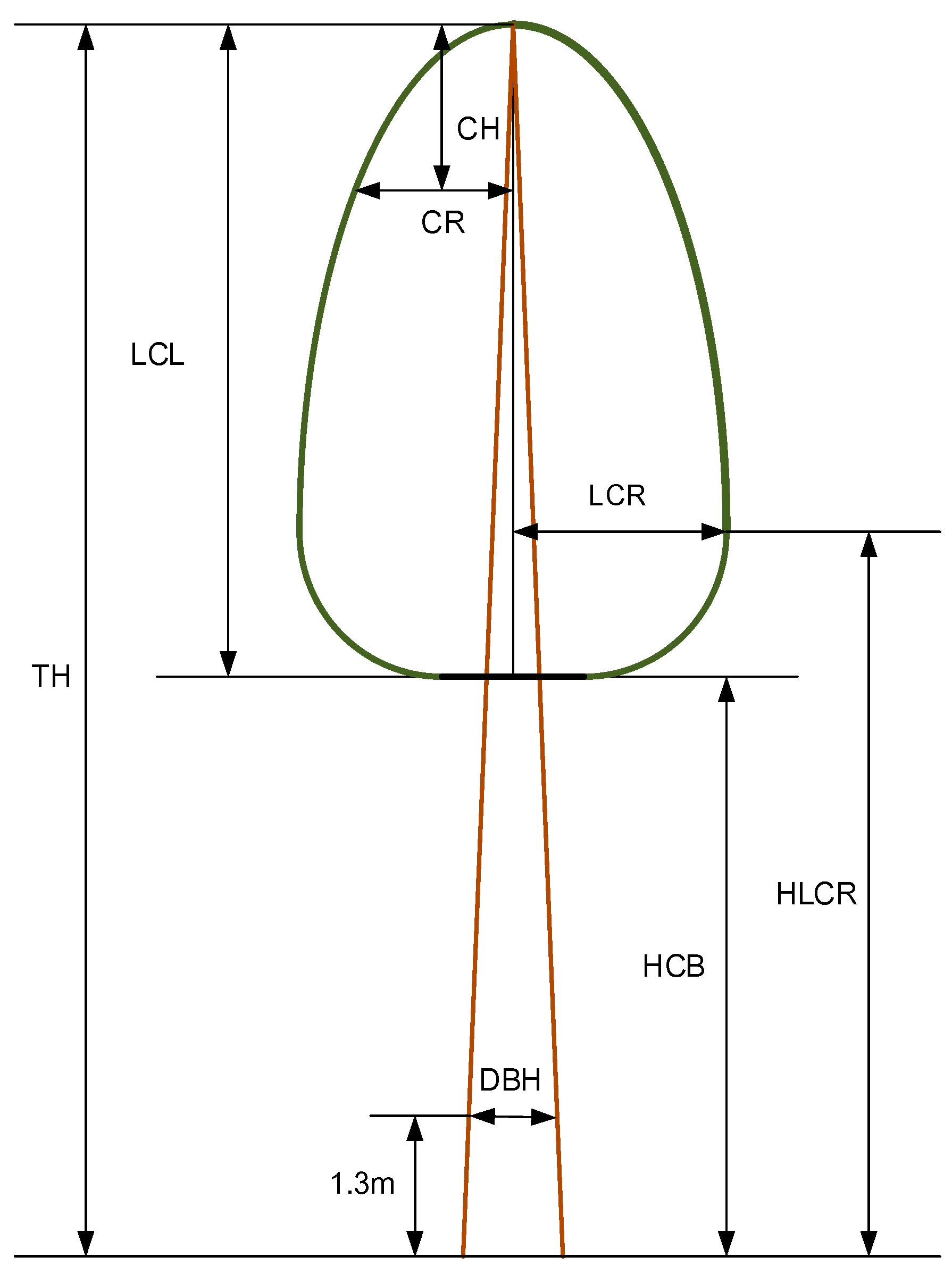
The data for this work came from the Dali and Lanxia forest farms in Fujian province, China. During the exploratory analysis, some obvious data errors were removed (25 trees). A total of 340 trees, with crowns distributed evenly over 65 pure, even-aged, and unthinned temporary plots (30 m × 30 m) were selected to determine the crown shape estimate of Chinese fir trees. For each tree, we measured the sample crown height from its top to crown base (CH, m) and measured the crown radius (CR, m) at each sampling height. (see Figure 1).

The crown data used in this study consisted of 1427 measured values, form 340 trees from Chinese fir stands with age ranging from 5 to 35 years. The tree factors used to establishment crown profile model should be selected according to the factors affecting the growth of trees. According to the relevant literature [2,3,4,6,11,34,35,37,38,44,47,51], the crown profile model is mainly affected by AGE, N, TH, DBH, LCL, CW, HCB, HLCR. In addition, in this study, we also defined the following composite tree factors: the tree crown length ratio, the HT to DBH ratio, and the tree crown fullness ratio. All the factors related to the crown and their descriptions are shown in

Table 1. Summary statistics of tree characteristic data for 340 sample trees.

Variable	Mean	Std Dev	Min	Max
AGE (year)	17	7	5	35
DBH (cm)	16.3	5.5	6.1	31.3
TH (m)	12.3	3.8	3.0	22.8
HCB (m)	6.5	3.2	0.3	16.3
CW (m)	3.5	1.0	1.1	7.3
LCL (m)	5.9	2.2	1.1	16.5
LCR (m)	1.8	0.5	0.5	3.7
TSC	0.8	0.1	0.4	1.3
CLR	0.5	0.2	0.2	0.9
CFR	0.7	0.3	0.1	2.0
CH (m)	2.9	2.1	0.0	12.4
CR (m)	1.8	1.9	0.0	6.6
RCH	0.41	0.31	0.00	0.90
RCR	1.00	0.70	0.00	3.27

.

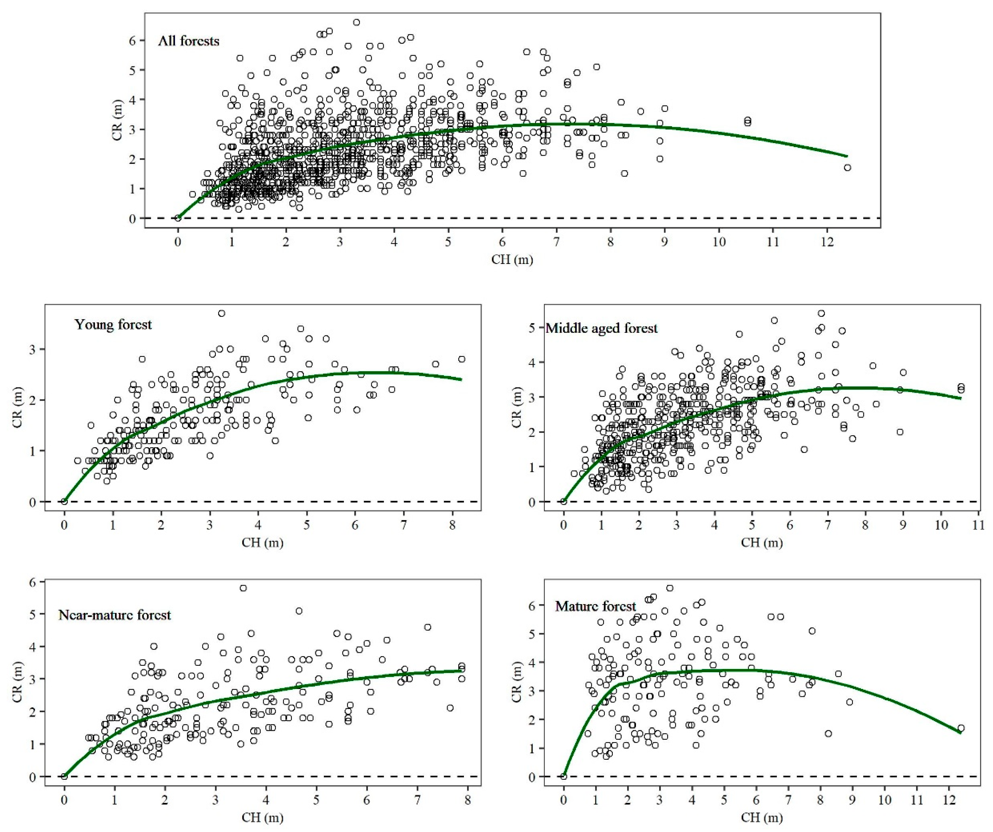
A detailed visual examination of the crown profiles suggested that sample trees from different age groups appeared to have a different crown form (Figure 2). Further research is required to improve the prediction effect of adding age variables in the crown profile equations or algorithms.

2.2. Parametric Regression Approach for the Crown Profile Model

We initially selected 25 crown profile models proposed in the literature with different numbers of parameters that had previously shown good performance (Table 2). The crown profile equations were estimated using nonlinear least-squares estimates through a Gauss–Newton algorithm, implemented in PROC MODEL (SAS Institute Inc., Cary, NC, USA, 2013) and we then compared the goodness-of-fit values. We screened for the parameters that passed t-test, and which had R-squared (R²) values greater than 60%, and selected these as the basic models.

Three different mean-covariance models were considered for estimation of means and covariances. The first is a saturated one in which all means and covariances are model parameters. The other two structured mean-covariance models use the same CR function to approximate means while characterizing covariances directly by using variance and correlation functions or indirectly via random effects within the framework of mixed-effects modeling [60]. For the nonlinear marginal model, parameters estimates and the subsequent analysis of the residual variance-covariance matrix were performed using the SAS macro %NLINMIX (SAS Institute, Inc., Cary, NC, USA, 2004). The %NLINIMX macro extends the fitting algorithm used in the GENMOD procedure by using a quadratic instead of a simple method in the moment estimation equation for the correlation parameters [61]. For the screened basic crown profile models, its parameter estimates and the subsequent analysis of the residual variance-covariance matrix were performed using the SAS macro %NLINMIX. To account for heteroscedastic, autocorrelated errors, the CAR(1) error structure was added to each CR equation for crown profile models (type = SP(POW)(RCH) specifies the covariance structure in Equation (1)), and the residuals were used to calculate weights (weight = 1/sqrt(${\widehat{\sigma }}^2$)).

$$\mathit{SP}(\mathit{POW})(c\text{-}\mathit{list})={\sigma }^2\left[\begin{array}{c}1\\ {\rho }^{d_{21}}\\ ⋮\\ {\rho }^{d_{m1}}\end{array}\begin{array}{c}{\rho }^{d_{12}}\\ 1\\ ⋮\\ {\rho }^{d_{m2}}\end{array}\begin{array}{c}\dots \\ \dots \\ ⋮\\ \dots \end{array}\begin{array}{c}{\rho }^{d_{1m}}\\ {\rho }^{d_{1m}}\\ ⋮\\ 1\end{array}\right]$$

(1)

where, ${\sigma }^2$ represents variances; $\rho$ represents correlation parameters; $d_{ij}$ the covariance between two observations depends on a distance metric; The c-list contains the names of the numeric variables used as coordinates to determine distance.

2.3. Artificial Intelligence Procedures for the Crown Profile Model

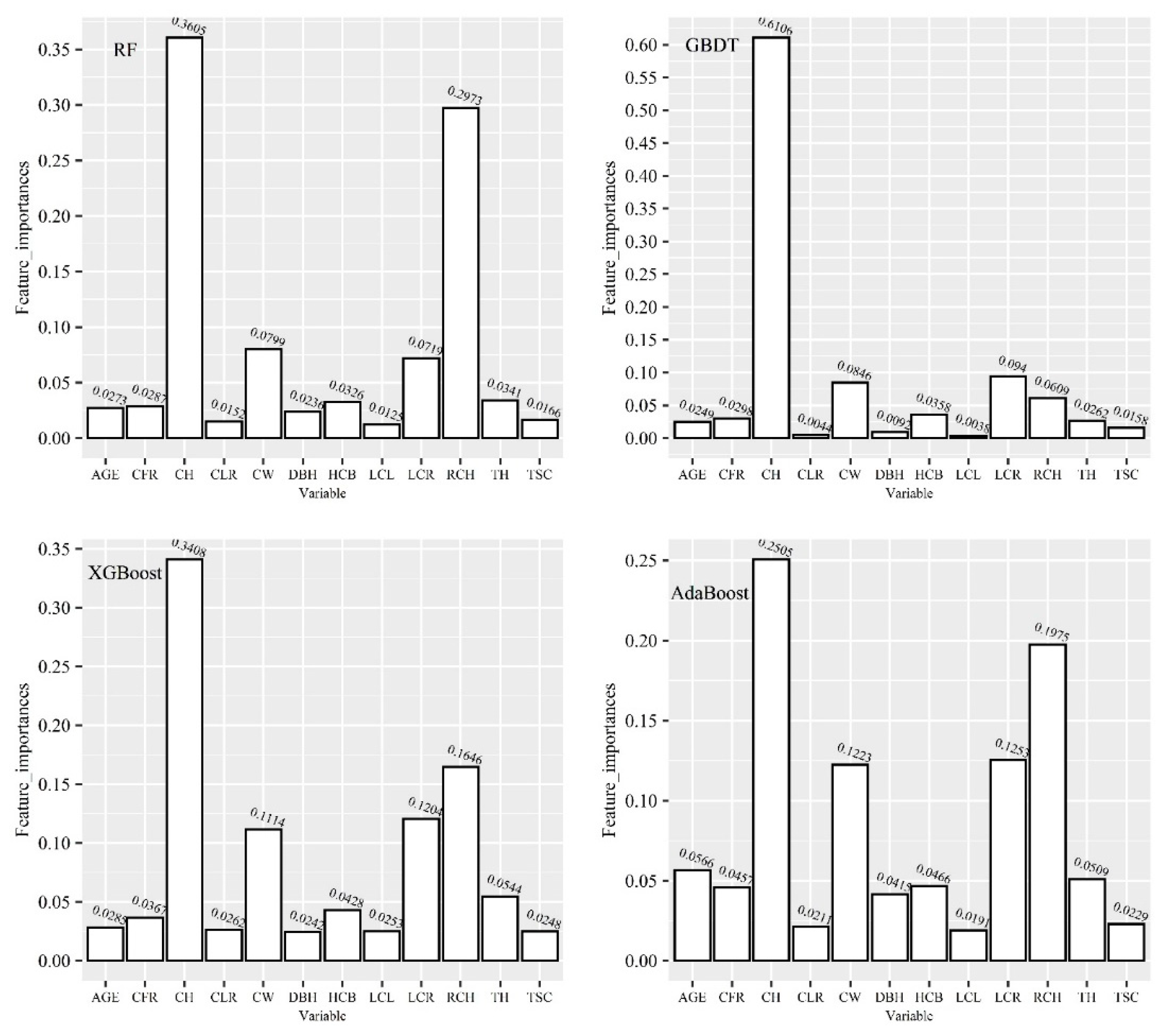
Six machine learning algorithms were used to construct the crown profile model of China fir trees in this paper, namely, artificial neural network (ANN), support vector regression (SVR), random forest (RF), adaptive boosting (AdaBoost), gradient boosting decision tree (GBDT) and extreme gradient boost (XGBoost) methods. Among these, RF, AdaBoost, GBDT and XGBoost belong to ensemble learning method. The objective is to predict CR (crown radius) at different relative crown height RCH.

$$CR=f(RCH;{\mathrm{X}}_i)$$

(2)

where, $f(RCH;{\mathrm{X}}_i)$ shows that some model or algorithm can depend on other variables ${\mathrm{X}}_i$ describing the tree.

From the model accuracy analysis, we should build the crown profile model that use all relevant variables (${\mathrm{X}}_i:$ DBH, TH, AGE, HCB, CW, LCL, LCR, TSC, CLR, CFR, CH) as input. From the model practicality analysis, we should train an AI algorithm that would use only standard forestry measures (${\mathrm{X}}_i:$ TH, DBH and AGE) as input. Considering different application scenarios, we trained these AI algorithms with two strategies for input variables: one is multivariable RCH, DBH, TH, AGE, HCB, CW, LCL, LCR, TSC, CLR, CFR, CH as inputs, and the other is only standard forestry measures as inputs.

ANN: ANN, also called a Multi-Layer Perceptron (MLP), achieves the goal of prediction through building a multilayer network. A typical neural network usually consists of an input layer, hidden layer and output layer. Based on different learning tasks, the number of hidden layers can reach any depth, and the output of each hidden layer is transformed by the activation function [62,63].

SVR: Support vector regression assumes that the allowable deviation between f(x) and y is at most ε, and the loss is calculated only when the absolute value of the difference between f(x) and y is greater than ε. At this time, it is equivalent to building an interval band with a width of 2ε with f(x) as the center. If the training sample falls into the interval band, the prediction is considered correct. It specifies the epsilon-tube within which no penalty is associated in the training loss function with points predicted within a distance εfrom the actual value.

RF: RF is an ensemble learner consisting of a collection of weak base learners (decision trees). By combining several weak base learners, the result can be achieved through voting or taking the mean value, which makes the results of the overall model have high accuracy and generalization performance [64].

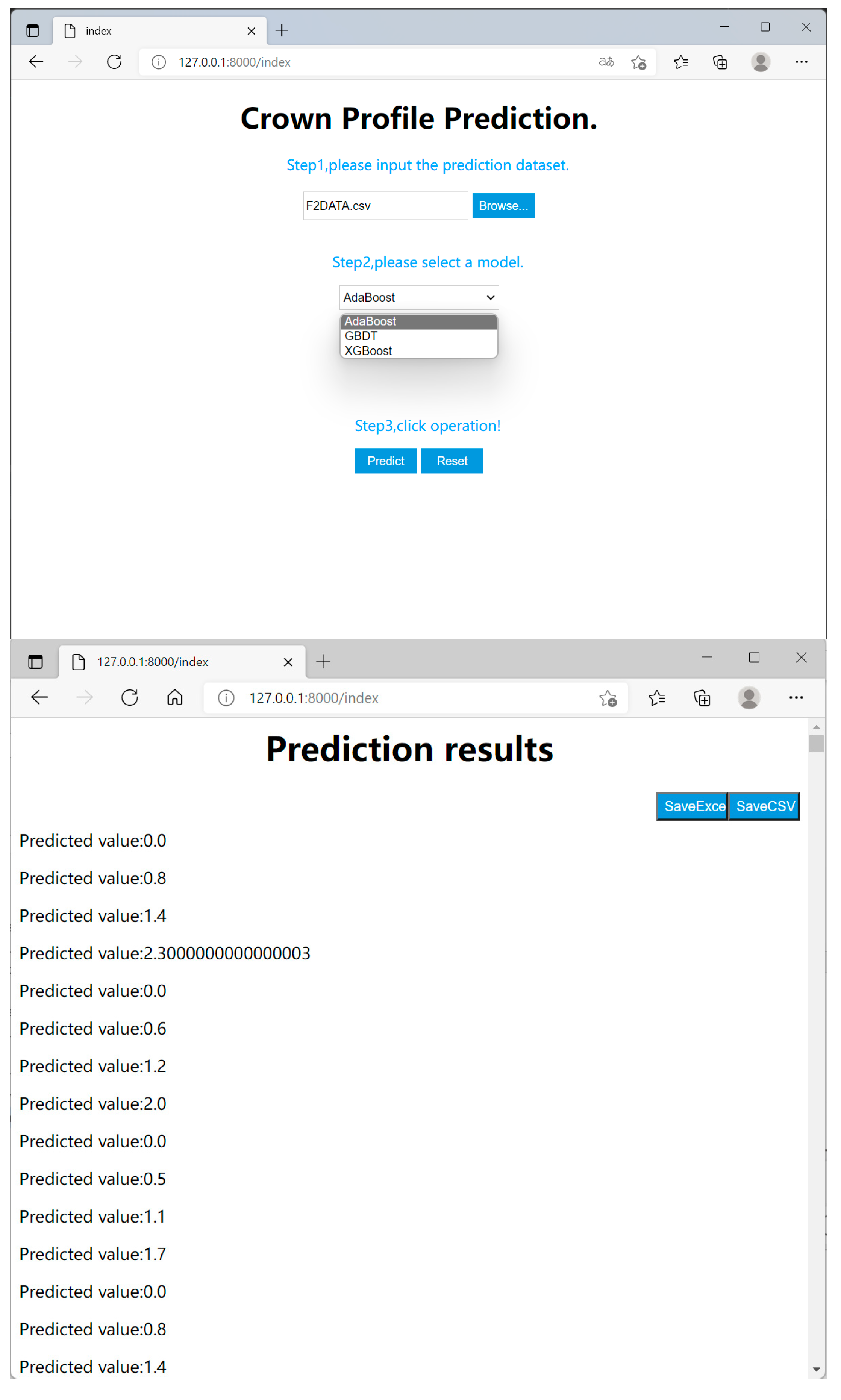
AdaBoost: AdaBoost is also an ensemble learning method that combines several weak learners into one strong learner to improve regression accuracy [65].

Table 2. Crown profile equations.

Model	Equation	Variable	Parameter	Reference
1	$CR=LCR{(1-RCH)}^{a_0}$	RCH, LCR	$a_0$	[34]
2	$CR=LCR{(1-(1-RC{H)}^2)}^{a_0}$	RCH, LCR	$a_0$	[35]
3	$CR=a_{0}RC{H}^{a_1}{(1-RCH)}^{a_2}$	RCH	$a_0,a_1,a_2$	[37]
4	$CR=a_0(\frac{RCH}{RCH-2})+a_{1}RCH$	RCH	$a_0,a_1$	[23]
5	$CR=a_0+a_{1}H+a_{2}C{H}^2+a_3\ast DBH\times CH+a_4\mathrm{DBH}\times C{H}^2+a_{5}TH\times CH+a_6\mathrm{TH}\times C{H}^2+a_7\mathrm{LCL}$	CH, DBH, TH, LCL	$$\begin{gathered} a_0,a_1,a_2,a_3,a_4, \\ {a}_5,a_6,a_7 \end{gathered}$$	[2]
6	$CR=LCR(exp(a_0+a_1(1-RCH)+a_2(1-RCH){}^2))$	RCH, LCR	$a_0,a_1,a_2$	[3]
7	$CR=LCR(a_0(\frac{RCH}{RCH-2})+a_{1}RCH)$	RCH, LCR	$a_0,a_1$	[4]
8	$CR=LCR(a_0(\frac{RCH}{RCH-2})+a_1{(RCH)}^{a_2})$	RCH, LCR	$a_0,a_1$	[48]
9	$CR=LCR(a_0+a_1(1-RCH)+a_2(1-RCH){}^2+a_3(1-RCH){}^3)$	RCH, LCR	$a_0,a_1,a_2,a_3$	[4]
10	$CR=a_0\frac{{(1-RCH)}^{a_1-1}RC{H}^{a_2-1}}{\beta (a_1,a_2)}$	RCH	$a_0,a_1,a_2$	[51]
11	$CR=a_0(\frac{a_2}{a_1}){(\frac{1-RCH}{a_1})}^{a_2-1}exp(-{(\frac{1-RCH}{a_1})}^{a_2})$	RCH	$a_0,a_1,a_2$	[51]
12	$CR=a_{0}RC{H}^{a_1}exp(a_2\ast RCH)$	RCH	$a_0,a_1,a_2$	[45]
13	$CR=DB{H}^{a_0}RC{H}^{a_1+a_{2}CLR}exp((a_3+a_{4}TSC)RCH)$	RCH, DBH, CLR, TSC	$a_0,a_1,a_2,a_3,a_4$	[45]
14	$CR=(a_{0}DB{H}^{a_1})(\frac{1-{(1-RCH)}^{0.5}}{1-{(a_{2}CL{R}^{a_3})}^{0.5}})+a_4(1-RCH)+a_5(exp(\frac{1}{TSC})(1-RCH))$	RCH, DBH, CLR, TSC	$a_0,a_1,a_2,a_3,a_4,a_5$	[45]
15	$CR=(a_0+a_1\ast DBH)RCH+(a_2+a_{3}CLR)RC{H}^2$	RCH, DBH, CLR	$a_0,a_1,a_2,a_3$	[45]
16	$$\begin{gathered} CR=(a_0+a_1\ast DBH)(\frac{(a_2+a_{3}CLR+a_{4}TSC)}{a_5+a_{6}DBH}){(\frac{1-RCH}{a_5+a_{6}DBH})}^{(a_2+a_{3}CLR+a_{4}TSC)-1} \\ exp(-{(\frac{1-RCH}{a_5+a_{6}DBH})}^{(a_2+a_{3}CLR+a_{4}TSC)}) \end{gathered}$$	RCH, DBH, CLR, TSC	$$\begin{gathered} a_0,a_1,a_2,a_3,a_4, \\ {a}_5,a_6 \end{gathered}$$	[11]
17	$CR=LCR(a_{0}LC{R}^{a1}+a_{2}LC{R}^{a_3}(1-RCH)+a_4(1-RCH){}^2)$	RCH, LCR	$a_0,a_1,a_2,a_3,a_4$	[66]
18	$CR=LCR(a_0+a_{1}exp(a_{2}LC{R}^{a_3}(1-RCH)))$	RCH, LCR	$a_0,a_1,a_2,a_3$	[66]
19	$CR=LCR(a_0\ast HC{B}^{a_1}(\frac{RCH}{RCH-2})+a_{2}HC{B}^{a_3}{(RCH)}^{a_4})$	RCH, LCR, HCB	$a_0,a_1,a_2,a_3,a_4$	[66]
20	$CR=LCR(a_0+a_{1}HC{B}^{a_2}(1-RC{H)}^{a_3})$	RCH, LCR, HCB	$a_0,a_1,a_2,a_3$	[66]
21	$CR=LCR((a_0+a_{1}AGE)((1-RCH)-1)+a_2((1-RCH){}^2-1)+a_3((1-RCH){}^3-1)+a_4((1-RCH){}^3-1))$	RCH, LCR, AGE	$a_0,a_1,a_2,a_3,a_4$	[66]
22	$CR=(a_0+a_{1}LCR)RCH+RC{H}^2$	RCH, LCR	$a_0,a_1$	[6]
23	$CR=a_0(1-exp(-(a_1+a_{2}LCR)RCH))$	RCH, LCR	$a_0,a_1,a_2$	[6]
24	$CR=(a_0+a_{1}LCR)RC{H}^{(a_2+a_{3}LCR)}$	RCH, LCR	$a_0,a_1,a_2,a_3$	[6]
25	$CR=(a_0+a_{1}LCR)\frac{{(1-RCH)}^{a_2-1}RC{H}^{(a_3+a_{4}LCR)-1}}{\beta (a_2,(a_3+a_{4}LCR))}$	RCH, LCR	$a_0,a_1,a_2,a_3,a_4$	[6]

Table 2. Crown profile equations.

Model	Equation	Variable	Parameter	Reference
1	$CR=LCR{(1-RCH)}^{a_0}$	RCH, LCR	$a_0$	[34]
2	$CR=LCR{(1-(1-RC{H)}^2)}^{a_0}$	RCH, LCR	$a_0$	[35]
3	$CR=a_{0}RC{H}^{a_1}{(1-RCH)}^{a_2}$	RCH	$a_0,a_1,a_2$	[37]
4	$CR=a_0(\frac{RCH}{RCH-2})+a_{1}RCH$	RCH	$a_0,a_1$	[23]
5	$CR=a_0+a_{1}H+a_{2}C{H}^2+a_3\ast DBH\times CH+a_4\mathrm{DBH}\times C{H}^2+a_{5}TH\times CH+a_6\mathrm{TH}\times C{H}^2+a_7\mathrm{LCL}$	CH, DBH, TH, LCL	$$\begin{gathered} a_0,a_1,a_2,a_3,a_4, \\ {a}_5,a_6,a_7 \end{gathered}$$	[2]
6	$CR=LCR(exp(a_0+a_1(1-RCH)+a_2(1-RCH){}^2))$	RCH, LCR	$a_0,a_1,a_2$	[3]
7	$CR=LCR(a_0(\frac{RCH}{RCH-2})+a_{1}RCH)$	RCH, LCR	$a_0,a_1$	[4]
8	$CR=LCR(a_0(\frac{RCH}{RCH-2})+a_1{(RCH)}^{a_2})$	RCH, LCR	$a_0,a_1$	[48]
9	$CR=LCR(a_0+a_1(1-RCH)+a_2(1-RCH){}^2+a_3(1-RCH){}^3)$	RCH, LCR	$a_0,a_1,a_2,a_3$	[4]
10	$CR=a_0\frac{{(1-RCH)}^{a_1-1}RC{H}^{a_2-1}}{\beta (a_1,a_2)}$	RCH	$a_0,a_1,a_2$	[51]
11	$CR=a_0(\frac{a_2}{a_1}){(\frac{1-RCH}{a_1})}^{a_2-1}exp(-{(\frac{1-RCH}{a_1})}^{a_2})$	RCH	$a_0,a_1,a_2$	[51]
12	$CR=a_{0}RC{H}^{a_1}exp(a_2\ast RCH)$	RCH	$a_0,a_1,a_2$	[45]
13	$CR=DB{H}^{a_0}RC{H}^{a_1+a_{2}CLR}exp((a_3+a_{4}TSC)RCH)$	RCH, DBH, CLR, TSC	$a_0,a_1,a_2,a_3,a_4$	[45]
14	$CR=(a_{0}DB{H}^{a_1})(\frac{1-{(1-RCH)}^{0.5}}{1-{(a_{2}CL{R}^{a_3})}^{0.5}})+a_4(1-RCH)+a_5(exp(\frac{1}{TSC})(1-RCH))$	RCH, DBH, CLR, TSC	$a_0,a_1,a_2,a_3,a_4,a_5$	[45]
15	$CR=(a_0+a_1\ast DBH)RCH+(a_2+a_{3}CLR)RC{H}^2$	RCH, DBH, CLR	$a_0,a_1,a_2,a_3$	[45]
16	$$\begin{gathered} CR=(a_0+a_1\ast DBH)(\frac{(a_2+a_{3}CLR+a_{4}TSC)}{a_5+a_{6}DBH}){(\frac{1-RCH}{a_5+a_{6}DBH})}^{(a_2+a_{3}CLR+a_{4}TSC)-1} \\ exp(-{(\frac{1-RCH}{a_5+a_{6}DBH})}^{(a_2+a_{3}CLR+a_{4}TSC)}) \end{gathered}$$	RCH, DBH, CLR, TSC	$$\begin{gathered} a_0,a_1,a_2,a_3,a_4, \\ {a}_5,a_6 \end{gathered}$$	[11]
17	$CR=LCR(a_{0}LC{R}^{a1}+a_{2}LC{R}^{a_3}(1-RCH)+a_4(1-RCH){}^2)$	RCH, LCR	$a_0,a_1,a_2,a_3,a_4$	[66]
18	$CR=LCR(a_0+a_{1}exp(a_{2}LC{R}^{a_3}(1-RCH)))$	RCH, LCR	$a_0,a_1,a_2,a_3$	[66]
19	$CR=LCR(a_0\ast HC{B}^{a_1}(\frac{RCH}{RCH-2})+a_{2}HC{B}^{a_3}{(RCH)}^{a_4})$	RCH, LCR, HCB	$a_0,a_1,a_2,a_3,a_4$	[66]
20	$CR=LCR(a_0+a_{1}HC{B}^{a_2}(1-RC{H)}^{a_3})$	RCH, LCR, HCB	$a_0,a_1,a_2,a_3$	[66]
21	$CR=LCR((a_0+a_{1}AGE)((1-RCH)-1)+a_2((1-RCH){}^2-1)+a_3((1-RCH){}^3-1)+a_4((1-RCH){}^3-1))$	RCH, LCR, AGE	$a_0,a_1,a_2,a_3,a_4$	[66]
22	$CR=(a_0+a_{1}LCR)RCH+RC{H}^2$	RCH, LCR	$a_0,a_1$	[6]
23	$CR=a_0(1-exp(-(a_1+a_{2}LCR)RCH))$	RCH, LCR	$a_0,a_1,a_2$	[6]
24	$CR=(a_0+a_{1}LCR)RC{H}^{(a_2+a_{3}LCR)}$	RCH, LCR	$a_0,a_1,a_2,a_3$	[6]
25	$CR=(a_0+a_{1}LCR)\frac{{(1-RCH)}^{a_2-1}RC{H}^{(a_3+a_{4}LCR)-1}}{\beta (a_2,(a_3+a_{4}LCR))}$	RCH, LCR	$a_0,a_1,a_2,a_3,a_4$	[6]

GBDT: GBDT is a boosting ensemble learning algorithm, but its the specific process is different from that of AdaBoost. The goal of GBDT is to continuously reduce the loss of each iteration [66].

XGBoost: XGBoost is an optimized distributed gradient boosting machine learning algorithms under the Gradient Boosting framework. A regularization technique is used in the XGBoost regression model. In the iterative optimization process, XGBoost uses the second-order approximation of the Taylor expansion of the objective function. Support parallelism is the flash point of XGBoost [67].

In terms of hyperparameter optimization, the grid search and random search are two generic approaches to parameter search, which are provided in scikit-learn by GridSearchCV and RandomizedSearchCV. Given the finite set of values for each hyperparameter, GridSearchCV exhaustively considers all hyperparameter sets combinations, whereas RandomizedSearchCV can sample a given number of candidates from a hyperparameter space with a specified distribution [68]. Considering the characteristics of different methods, in this paper we chose the strategy of combining the random and network search to simplify the required number of experimental iterations. Firstly, a random search was used to obtain the general direction in a large range of parameter space. Then, the results of random parameter selection were used as the basis for the following grid search. Different parameters and different preprocessing schemes were repeatedly compared, and the optimal hyperparameter set was finally screened out.

2.4. Model Evaluation and Validation

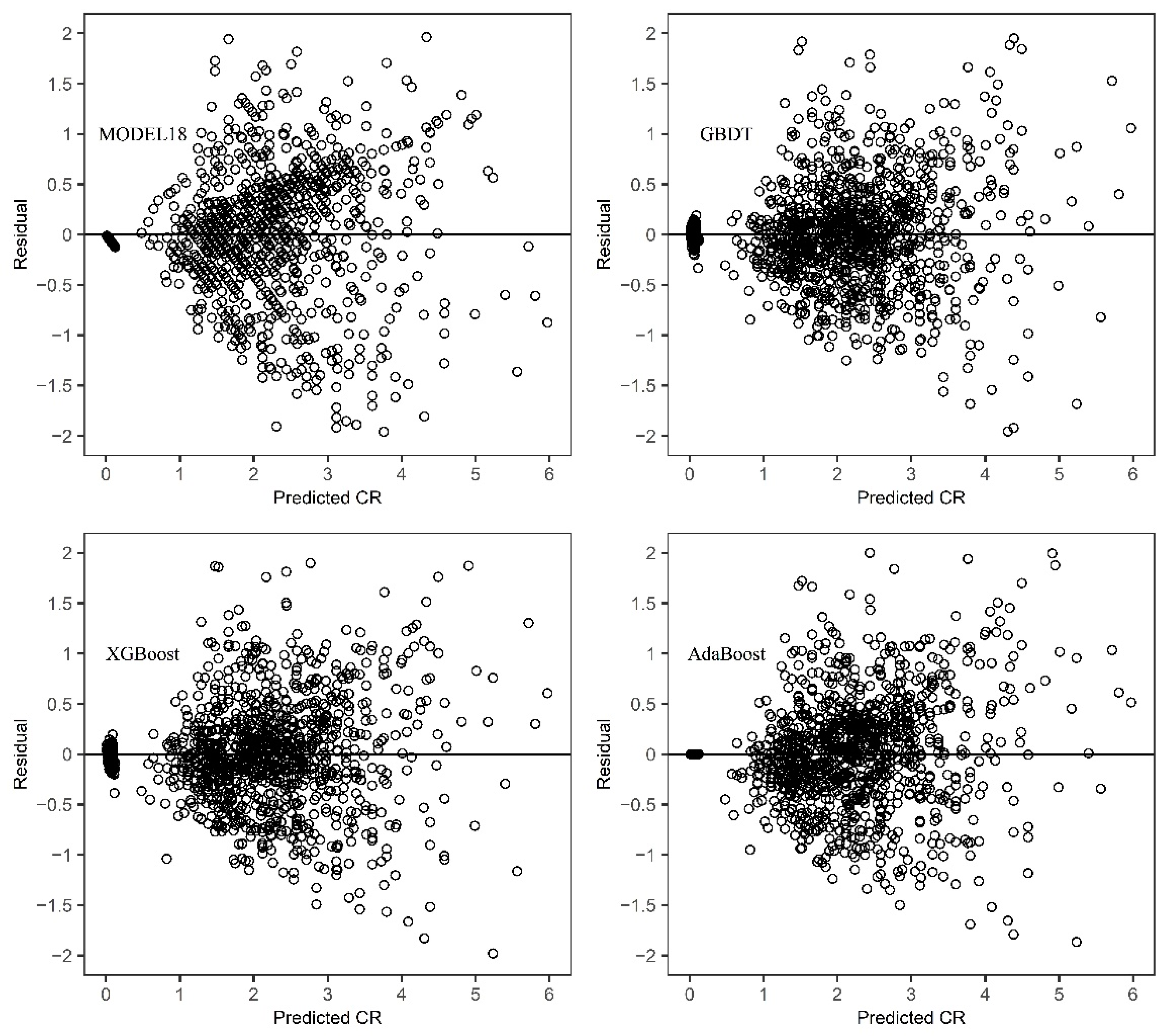
The way of dividing training set and test set judged whether the model has over fitting or under fitting problems. To assess the predictive accuracy of the estimated crown profile models, the leave-one-out approach based on tree level was selected for model validation. For N sample trees, each model was fitted N times. Each time, all the data points of one tree were removed from the fitting process, and predicted the values of CR were obtained for these using the coefficients estimated from the remaining data.

The performance indicators were calculated for both training and validation datasets. The evaluation criteria included the mean deviation (ME, Equation (3)), the mean absolute deviation (MAE, Equation (4)) [53] and the mean squared error (MSE, Equation (5)). We compared the goodness-of-fits using the root mean squared error (RMSE, Equation (6)), the R-squared value (R², Equation (7)), the Akaike Information Criterion (AIC, Equation (8)) and the Bayesian Information Criterion (BIC, Equation (9)).

$$ME=\frac{{{\displaystyle \sum }}_{i=0}^n(y_i-\widehat{y_i})}{n}$$

(3)

$$MAE=\frac{{{\displaystyle \sum }}_{i=1}^n\left|y_i-\widehat{y_i}\right|}{n}$$

(4)

$$MSE=\frac{{{\displaystyle \sum }}_{i=1}^n{(y_i-\widehat{y_i})}^2}{n}$$

(5)

$$RMSE=\sqrt{\frac{{{\displaystyle \sum }}_{i=1}^n{(y_i-\widehat{y_i})}^2}{n}}$$

(6)

$$R^2=1-\frac{{{\displaystyle \sum }}_{i=1}^n{(y_i-\widehat{y_i})}^2}{{{\displaystyle \sum }}_{i=1}^n{(y_i-\overline{y_i})}^2}$$

(7)

$$AIC=n\ln (\mathrm{MSE})+2\mathrm{k}$$

(8)

$$BIC=n\ln (MSE)+k\ln (n)$$

(9)

where $y_i$ represents the observed value; $\widehat{y_i}$ is the predicted value; n is the number of tree points, $\overline{y_i}$ is the mean value for the observed, and is the number of parameters in the model.

3. Results

3.1. Parametric Regression Approach for the Crown Profile Model

A nonlinear OLS summary of residual errors for all crown profile models is given in

Table 3. Nonlinear OLS summary of residual errors for 25 crown profile models.

Model	MSE	RMSE	R2	Parameter t-Test
MODEL1	1.2111	1.1005	0.3720	significant
MODEL2	1.0864	1.0423	0.1336	significant
MODEL3	0.9890	0.9945	0.2128	significant
MODEL4	0.7950	0.8916	0.5881	significant
MODEL5	0.6233	0.7895	0.6784	non-significant
MODEL6	0.5113	0.7151	0.7352	significant
MODEL7	0.4330	0.6580	0.7756	significant
MODEL8	0.9680	0.9838	0.2295	significant
MODEL9	0.4082	0.6389	0.7888	non-significant
MODEL10	0.9890	0.9945	0.2128	significant
MODEL11	0.9201	0.9592	0.5236	significant
MODEL12	0.9902	0.9951	0.2119	significant
MODEL13	0.7161	0.8462	0.4310	significant
MODEL14	0.8138	0.9021	0.5795	significant
MODEL15	0.6020	0.7759	0.6885	non-significant
MODEL16	0.7246	0.8512	0.6258	significant
MODEL17	0.3999	0.6324	0.7932	significant
MODEL18	0.3911	0.6254	0.7976	significant
MODEL19	0.4809	0.6935	0.6179	significant
MODEL20	0.3973	0.6303	0.7944	significant
MODEL21	0.3838	0.6195	0.8016	non-significant
MODEL22	0.6815	0.8255	0.6469	significant
MODEL23	0.4328	0.6579	0.7759	significant
MODEL24	0.4748	0.6891	0.6224	significant
MODEL25	0.4828	0.6948	0.6164	non-significant

Notes: non-significant, at least one parameter is non-significant.

. It can be seen from the table that the basic models screened were model 6, model 7, model 16, model 17, model 18, model 19, model 20, model 22, model 23 and model 24.

The screened basic crown profile models were estimated using the SAS macro %NLINMIX (code in Appendix A). Goodness-of-fit statistics for the crown profile models, accounting for a heteroscedastic, autocorrelated error structure, are given in

Table 4. Goodness-of-fit statistics of %NLINMIX for crown profile models.

Model	RMSE	R2	AIC	BIC
MODEL6	0.7146	0.7350	−953.04	−937.25
MODEL7	0.6594	0.7744	−1184.63	−1174.10
MODEL17	0.6381	0.7887	−1272.19	−1245.87
MODEL18	0.6257	0.7969	−1330.29	−1309.23
MODEL23	0.6664	0.7695	−1152.19	−1136.40

. Models that %NLINMIX did not converge (e.g., model 16, model 19, model 24) and for which the parameters were not significantly different from zero ($\mathsf{\alpha }$ = 0.05) (e.g., model 20 and model 24) were removed from the model and are not shown in this table. All five crown profile models are accurate as indicated by the fit statistics for the entire crown, with model 18 showing slightly better results (Table 4).

However, comparing the two fitting results of the PROC MODEL and the %NLINMIX macro, it can be seen that the %NLINMIX macro tended to have less prediction accuracy than the PROC MODEL. Comparing the fitting parameters of model 18 under the two methods, we found that by comparing the parameters obtained by fitting the PROC MODEL and the %NLINMIX macro (

Table 5. The parameter estimates for model 18 using the PROC MODEL and the %NLINMIX macro.

Parameter	PROC MODEL			%NLINMIX Macro
	Estimate	S.E.	CV	Estimate	S.E.	CV
a0	1.7650	0.0111	0.0063	1.7619	0.0345	0.0196
a1	−0.0969	0.0047	−0.0488	−0.0900	0.0152	−0.1689
a2	2.8884	0.0428	0.0148	3.0174	0.1567	0.0519
a3	−0.0015	0.0005	−0.3367	−0.0238	0.0118	−0.4952

Notes: S.E., standard error; CV, coefficient of variation.

), the CV values of the former parameters a0, a1, a2 and a3 were smaller, indicating that these parameters are more stable and credible. Consequently, we choose the %NLINMIX macro over the PROC MODEL because of its suitability for hierarchically structured data (e.g., multiple measurements within a tree and multiple trees within a sample plot).

3.2. Artificial Intelligence Procedures for the Crown Profile Model

Table 6. The hyper-parameter optimization of artificial intelligence procedures for the crown profile model.

Model	Python Package	Hyper-Parameter Value	Hyper-Parameter Value
		(Strategy 1)	(Strategy 2)
MLP	sklearn.neural_network.MLPRegressor	hidden_layer_sizes = (180, 180, 180, 180, 180, 180, 180, 180, 180),	hidden_layer_sizes = (180, 180, 180, 180, 180, 180, 180, 180, 180),
		activation = ‘relu’,	activation = ‘relu’,
		solver = ‘adam’,	solver = ‘adam’,
		learning_rate_init = 0.01,	learning_rate_init = 0.007,
		max_iter = 247	max_iter = 90
SVR	sklearn.svm.SVR	kernel = ‘rbf’,	kernel = ‘linear’,
		epsilon = 0.1,	epsilon = 0.01,
		C = 1	C = 1
RF	sklearn.ensemble.RandomForestRegressor	n_estimators = 218,	n_estimators = 216,
		max_depth = 10,	max_depth = 8,
		min_samples_leaf = 1,	min_samples_leaf = 1,
		min_samples_split = 2,	min_samples_split = 7,
		max_features = ‘sqrt’,	max_features = ‘sqrt’,
		bootstrap = True	bootstrap = True
AdBoost	sklearn.ensemble.AdaBoostRegressor	n_estimators = 1215, max_depth = 18,	n_estimators = 924, max_depth = 15,
		min_samples_split = 5,	min_samples_split = 2,
		min_samples_leaf = 11,	min_samples_leaf = 10,
		max_features = ‘sqrt’,	max_features = ‘auto’,
		learning_rate = 0.01	learning_rate = 0.01
GBDT	sklearn.ensemble.GradientBoostingRegressor	n_estimators = 804,	n_estimators = 100,
		max_depth = 5,	max_depth = 2,
		min_samples_leaf = 7,	min_samples_leaf = 1,
		min_samples_split = 3,	min_samples_split = 2,
		learning_rate = 0.01,	learning_rate = 0.1,
		loss = ‘ls’	loss = ‘huber’
XGBoost	xgboost.XGBRegressor	n_estimators = 894,	n_estimators = 959,
		max_depth = 6,	max_depth = 1,
		colsample_bytree = 0.9,	colsample_bytree = 0.1,
		min_child_weight = 4,	min_child_weight = 5,
		gamma = 1,	gamma = 0.1,
		learning_rate = 0.01,	learning_rate = 0.01,
		reg_alpha = 10−5,	reg_alpha = 10−5,
		subsample = 0.5	subsample = 0.5

presents the hyper-parameter optimization results obtained from the six machine learning algorithms used to construct the crown profile model. For the MLP, some hyper-parameter values of the two strategies are consistent. For example, there were nine hidden layers, the number of neurons in each hidden layer was 180, and the activation function for the hidden layer was the rectified linear unit function (‘relu’). For the SVR from the model accuracy analysis (Strategy 1), the ‘rbf’ kernel type was used in the algorithm. The two free parameters C and epsilon in the SVR model took the values of 1 and 0.1, respectively. From the model practicality analysis (Strategy 2), The three free parameters kernel, C and epsilon in the SVR model took the values of ‘linear’, 1 and 0.1, respectively. For the four ensemble learning methods, there are obvious differences in the value of hyper-parameter between the algorithms of strategy 1 and strategy 2. Ensemble learning algorithms combine several decision tree models to help reduce bias and variance, the hyper-parameters ‘n_estimators’, ‘max_depth’, ‘min_samples_leaf’, ‘min_samples_split’ and ‘max_features’ all appear in the ensemble learning models. The proper combination of these hyper-parameters improved the prediction accuracy of the model.

Table 7. Fitting statistics for 6 artificial intelligence procedures (MLP, SVR, RF, AdaBoost, GBDT and XGBoost).

Strategy	Model	RMSE	R2	AIC	BIC	Rank
Strategy 1	MLP	0.5303	0.8540	−1764.08	−1643.02	5
	SVR	0.6144	0.8041	−1368.21	−1310.32	6
	RF	0.2664	0.9632	−3740.97	−3651.49	2
	AdaBoost	0.2933	0.9554	−3470.86	−3391.91	3
	GBDT	0.2592	0.9652	−3811.89	−3701.36	1
	XGBoost	0.2996	0.9534	−3393.42	−3272.36	4
Strategy 2	MLP	0.7862	0.6793	−640.54	−519.49	5
	SVR	0.8934	0.5858	−299.74	−241.84	6
	RF	0.4676	0.8866	−2135.6	−2046.12	2
	AdaBoost	0.3594	0.9330	−2890.92	−2811.97	1
	GBDT	0.6036	0.8109	−1398.53	−1288.01	3
	XGBoost	0.7442	0.7126	−797.12	−676.06	4

Note: Rank is the rating of the test statistic (RMSE, R2, AIC and BIC), the smaller the rating value, the better the model prediction result.

summarizes the performance indicators of MLP, SVR, RF, AdaBoost, GBDT and XGBoost for training. As shown in Table 7, artificial intelligence procedures for the crown profile model appeared to have the best performance and the highest efficiency from the model accuracy analysis (Strategy 1). The most striking result to emerge from the data is that the four ensemble learning approaches also presented the best performance for crown profile estimation for all the evaluated criteria. Surprisingly, AdaBoost had a high goodness of fit (R2 = 0.9330) from the model practicality analysis (Strategy 2). After the hyperparameter optimization of the random search and grid search, the goodness of fit of the model was more than 0.9.

3.3. Evaluation of Prediction Accuracy

3.3.1. Prediction Accuracy of the Crown Profile Model

The original data (340 trees) were randomly divided into two groups, 80% for the training set, and the other 20% as the validation set. The R² of the six crown profile models based on artificial intelligence procedures were shown in

Table 8. Evaluation results of dataset splitting of the six crown profile models based on artificial intelligence procedures.

Model	Training Dataset	Validation Dataset
MLP	0.8884	0.5095
SVR	0.8234	0.7159
RF	0.9624	0.9014
AdaBoost	0.9613	0.8915
GBDT	0.9717	0.9397
XGBoost	0.9580	0.9060

. The test results showed that the RF, AdaBoost, GBDT and XGBoost had no over-fitting phenomenon; MLP and SVR algorithms were slightly over fitted.

From the model accuracy analysis,

Table 9. Comparison of test results of crown profile models for China fir trees with different modeling methods.

Model	ME (Rank)	MAE (Rank)	MSE (Rank)	Sum Rank (Rank)
MODEL18	−0.0016 (1)	0.4235 (5)	0.3918 (5)	11 (2)
MLP	0.0093 (3)	0.4292 (6)	0.4138 (6)	15 (5)
SVR	0.0975 (7)	0.5336 (7)	0.5423 (7)	21 (6)
RF	0.0171 (5)	0.3396 (4)	0.2623 (4)	13 (4)
AdaBoost	0.0203 (6)	0.3306 (3)	0.2506 (3)	12 (3)
GBDT	0.0113 (4)	0.3250 (1)	0.2450 (1)	6 (1)
XGBoost	0.0082 (2)	0.3291 (2)	0.2464 (2)	6 (1)

Note: Rank is the rating of the test statistic (ME, MAE and MSE), the smaller the rating value, the better the model prediction result.

presents the leave-one-out results based on tree-level cross validation for the crown profile models. We summarized the model efficiency estimates of the parametric regression approach and artificial intelligence procedures. The crown equation designated as model 18 showed an intermediate performance in terms of estimation, whereas GBDT and XGBoost appeared to have the best performance and higher efficiency.

As for ME, the validation results showed that the crown equation was the most precise and efficient modeling technique for estimation, with an ME of −0.0016 m for model 18, 0.0082 m for XGBoost and 0.0093 m for MLP. In terms of the MAE and the MSE, the prediction effect of model 18 (the best model in the parametric regression approach) was slightly worse than that of these ensemble learning models, but better than that of the other machine learning models (MLP and SVR). The model 18 had the smallest ME, and GBDT had the smallest MAE and MSE for the entire crown. The single most striking observation to emerge from the data comparison was that the ensemble learning models appeared to have the best performance and the highest efficiency.

Further comparison among the four ensemble learning models showed that the RF method also presented the worst performance in terms of estimations for all the evaluated criteria. Among the other three models, XGBoost had the smallest ME (0.0082), GBDT had the smallest MAE (0.3250) and MSE (0.2450).

Figure 3 shows the features importance of each variable of the four ensemble learning algorithms (RF, GBDT, XGBoost and AdaBoost). Variable CH had the highest importance among the four algorithms. For the RF algorithm, the features (variables) that had a great impact on the construction of the crown profile model were CH, RCH, CW and LCR. For the XGBoost algorithm and the AdaBoost algorithm, in addition to CH, RCH, CW and LCR, other variables also have a certain degree of impact on crown contours. CH, CW and LCR were important features affecting crown profile model based on the GBDT algorithm.

3.3.2. Performance of the Crown Profile Model

Combined with the fitting and testing effects, we selected four models model 18, GBDT, XGBoost and AdaBoost to analyze the performance of the crown profile model. We plotted the residuals of CR predictions versus CR predictions (Predicted CR) for MODEL18, GBDT, XGBoost and AdaBoost (Figure 4). The residual graphs of the four models showed no heteroscedasticity except for the special point at CH = 0 at the top of the tree canopy. It can be seen intuitively that among the four models, model 18 had a large residual range. The residuals of algorithms GBDT, XGBoost and AdaBoost were concentrated between −1 and 1.

The residual results of the optimal model (GBDT) in each period of Chinese fir growth are shown in Figure 5. The optimal model in each period met the statistical test requirements, and the residuals in each growth period of Chinese fir were all distributed between ±2.0, which was smaller than the statistical range. It can also be seen intuitively that the model performed better in young forest, middle aged forest and near-mature forest. The residuals globally increased with tree age. Therefore, the optimal model in each growth period could fully represent the crown profile of different age groups of Chinese fir trees.

Four trees (a young forest tree, middle aged forest tree, near-mature forest tree and mature forest tree) with different sizes from three plots with different stand age were selected and the fitted outer crown profile curves against the observed crown radius of these four trees are shown in Figure 6. We can see that the crown profile tends to expand with age. At a young age and in middle age, the overall crown profile is straight, and at a young age, the crown length is the longest out of the whole growth period. In the near-mature period, the middle and lower crown are more prominent, and the overall shape is fuller and similar to parabolic shape. In the mature forest period, the lower part is prominent, and the crown length is the shortest in the whole growth process of the Chinese fir.

3.3.3. Application of the Crown Profile Model

We have presented two approaches to crown profile model for application in forestry practice. For the mathematical equation (model 18), the variable LCR (half the CW) is not a commonly used measurement factor, and the form of the equation predicting CW from DBH follows that of Qiao Chen (Equation (10), R² = 0.6606) [51]. Then once the DBH of the tree is known, the crown profile of the corresponding tree is obtained.

$$\mathrm{CW}=0.8367{\mathrm{DBH}}^{0.5079}$$

(10)

Compared with traditional equation models, the biggest problem with procedural models is how to simplify calls and make it easier to use. For artificial intelligence procedures (GBDT, XGBoost and AdaBoost), we developed Web programs based on the requirement of a lightweight design, and Tornado was used as a Web server to simplify and improve the access and application of the crown profile models. When invoking the model, one enters the interactive page of the Chinese fir plantation crown profile calculation as shown in Figure 7; imports the file information, including the crown model’s independent variables, in the file dialog box; selects GBDT, XGBoost, or AdaBoost Model; and clicks the “Predict” button to obtain the prediction results.

4. Discussion

The most obvious finding to emerge from the analysis was that ensemble learning method has strong nonlinear problem learning ability and the flexibility to analyze longitudinal data relating to crown profiles. In forest surveys, the crown profile database or stem form database belongs to the category of hierarchical data, which produces multicollinearity, autocorrelation and heteroscedasticity [48,69,70,71]. These problems may seriously affect the standard errors of the coefficients, thereby invalidating statistical tests using t or F distributions and confidence intervals [72,73]. Artificial Intelligence procedures for the crown profile model offer some advantages when compared to statistical modeling techniques. Firstly, there is no need to assume an underlying data distribution (as is usually done in statistical modeling). Secondly, it can implicitly detect complex nonlinear relationships between output and input variables [74]. Compared with artificial Intelligence procedures (Table 7 and Table 9), the ensemble learning approaches presented the best performance in both training and evaluation. Table 8 showed that the performance of the GBDT, XGBoost and AdaBoost ensemble learning algorithms for the Chinese fir crown profile models was superior to that of the other algorithms. It is important to mention, however, some barriers to the widespread successful application of artificial intelligence in forestry. One limitation is that artificial intelligence algorithms can easily incur problems of data overfitting [74,75]. Another serious limitation is that the black-box operation without an explanation mechanism make the process of establishing causation between inputs and outputs unclear, implying limited ecological interpretability [76,77].

There is an age variable in the crown profile model (model 21). As explained above, the related literature shows that age has a certain influence on the crown profile. Figure 5 showed that the residuals in each growth period of Chinese fir trees were obviously different. Moreover, the fitted outer crown profile curves showed different shape characteristics in the four age periods (Figure 6). The age variable significantly contributed to the variations in the crown profile model. For plantation, it is necessary to study the dynamic crown profile model because of the easy availability of age data and its close correlation with crown profile. The prediction bias can be reduced through the integration of all kinds of variability into the crown width models [78,79]. Thus, we selected TH, CH, DBH, LCL, RCH, CW, LCR, TSC, CLR, CFR and AGE variables on the tree level as the input variables. The results (Table 9) showed that crown profile models with these variables presented better fittings than simpler models with few variables. Moreover, current models may be biased when applied at a large scale as the crown profile is largely influenced by site quality, stand density, and random variabilities caused by various stochastic factors that vary from stand to stand [10]. This suggests that the most suitable model may consider multiple factors.

Crown profile 3D visualization is useful for forest crown stretch space determination, tree crown competition index establishment, and reference construction to analyze tree crown production efficiency [38]. 3D crown profile displays based on the proposed models represent an operational method. Driven by the crown profile model, the constructed digital 3D model can intuitively display the size of the tree crown under different growth conditions and the degree of overlap of tree crowns among individual trees, which is especially suitable for qualitative and quantitative descriptions of tree crown morphology and the analysis of trees’ spatial distribution patterns in the visualization process of plantation forest management [38,46]. Crown profile models and 3D tree visualization can be closely combined and applied to forest management visualization, which is a direction of follow-up research.

5. Conclusions

Based on an analysis of the disadvantages of crown profile modeling, in this study we developed two promising modeling methods (a nonlinear marginal model and ensemble learning), which represent new and essential explorations in the study of parametric and nonparametric methods. We concluded that (1) the parameters of the nonlinear marginal model were more stable and credible; (2) the ensemble learning approaches, especially AdaBoost, GBDT and XGBoost, presented the best performance for crown profile estimation for all the evaluated criteria; (3) the leave-one-out cross validation results showed that the crown equation model 18 (the best model in the parametric regression approach) displayed an intermediate performance for estimation, whereas the GBDT method appeared to have the best performance and the highest efficiency. In conclusion, the following are the highlights of the study:

• For the crown profile equation, parameter estimates for the nonlinear marginal model were performed using the SAS macro %NLINMIX.
• Ensemble learning procedures can deal with complex nonlinear relationship and show strong prediction ability when predicting the crown profile.
• We compared the properties of modeling and predictions for crown profiles between the ensemble learning method and the nonlinear marginal model method.

It should be pointed out that crown profiles based on artificial intelligence procedures should be used in systems to realize the dynamic updating of models. Our next research goal is to develop a prototype of an expert-assisted afforestation decision support system, based online, with the main function of realizing model invocation and automatic updates, which could be widely used in forestry practice. For ensemble learning regression, this study aimed to explore the application of bootstrap ensemble learning regression on the modeling and prediction of crown profiles. Further research can explore the stacking of ensemble learning regression or deep learning regression algorithm for crown profile models.

References

1. Weiskittel, A.R. Forest growth and yield models for intensively managed plantations. In The Management of Industrial Forest Plantations; Springer: Dordrecht, The Netherlands, 2014; pp. 61–90. [Google Scholar]
2. Roeh, R.L.; Maguire, D.A. Crown profile models based on branch attributes in coastal Douglas-fir. For. Ecol. Manag. 1997, 96, 77–100. [Google Scholar] [CrossRef]
3. Hann, D.W. An adjustable predictor of crown profile for stand-grown Douglas-fir trees. For. Sci. 1999, 45, 217–225. [Google Scholar]
4. Crecente-Campo, F.; Marshall, P.; LeMay, V.; Die’guez-Aranda, U. A crown profile model for Pinus radiata D. Don in northwestern Spain. For. Ecol. Manag. 2009, 257, 2370–2379. [Google Scholar] [CrossRef]
5. Fengri, L. Modeling Crown Profile of Larix olgensis Trees. Sci. Silvae Sin. 2004, 40, 16–24. [Google Scholar]
6. Quan, Y.; Li, M.; Zhen, Z.; Hao, Y.; Wang, B. The Feasibility of Modeling the Crown Profile of Larix olgensis Using Unmanned Aerial Vehicle Laser Scanning Data. Sensors 2020, 20, 5555. [Google Scholar] [CrossRef] [PubMed]
7. Attocchi, G.; Skovsgaard, J.P. Crown radius of pedunculate oak (Quercus robur L.) depending on stem size, stand density and site productivity. Scand. J. For. Res. 2015, 30, 289–303. [Google Scholar]
8. Fu, L.; Sun, H.; Sharma, R.P.; Lei, Y.; Zhang, H.; Tang, S. Nonlinear mixed-effects crown width models for individual trees of Chinese fir (Cunninghamia lanceolata) in south-central China. For. Ecol. Manag. 2013, 302, 210–220. [Google Scholar] [CrossRef]
9. Fu, L.; Zhang, H.; Sharma, R.P.; Pang, L.; Wang, G. A generalized nonlinear mixed-effects height to crown base model for Mongolian oak in northeast China. For. Ecol. Manag. 2017, 384, 34–43. [Google Scholar] [CrossRef]
10. Sharma, R.P.; Bílek, L.; Vacek, Z.; Vacek, S. Modeling crown width–diameter relationship for Scots pine in the central Europe. Trees 2017, 31, 1875–1889. [Google Scholar] [CrossRef]
11. Gao, H.; Dong, L.; Li, F. Modeling variation in crown profile with tree status and cardinal directions for planted Larix olgensis Henry trees in Northeast China. Forests 2017, 8, 139. [Google Scholar] [CrossRef] [Green Version]
12. Larson, P.R. Stem Form Development of Forest Trees. For. Sci. 1963, 9, a0001-42. [Google Scholar] [CrossRef]
13. Assmann, E. The Principles of Forest Yield Study: Studies in the Organic Production, Structure, Increment and Yield of Forest Stands; Pergamon Press: Oxford, UK, 1970. [Google Scholar]
14. Burkhart, H.E.; Walton, S.B. Incorporating crown ratio into taper equations for loblolly pine trees. For. Sci. 1985, 31, 478–484. [Google Scholar]
15. Valenti, M.A.; Cao, Q.V. Use of crown ratio to improve loblolly pine taper equations. Can. J. For. Res. 1986, 16, 1141–1145. [Google Scholar] [CrossRef]
16. Muhairwe, C.K.; Lemay, V.M.; Kozak, A. Effects of adding tree, stand, and site variables to Kozak’s variable-exponent taper equation. Can. J. For. Res. 1994, 24, 252–259. [Google Scholar] [CrossRef]
17. Leites, L.P.; Robinson, A.P. Improving taper equations of loblolly pine with crown dimensions in a mixed-effects modeling framework. For. Sci. 2004, 50, 204–212. [Google Scholar]
18. Jiang, L.; Brooks, J.R.; Hobbs, G.R. Using crown ratio in yellow-poplar compatible taper and volume equations. North. J. Appl. For. 2007, 24, 271–275. [Google Scholar] [CrossRef] [Green Version]
19. Jiang, L.C.; Liu, R.L. Segmented taper equations with crown ratio and stand density for Dahurian Larch (Larix gmelinii) in Northeastern China. J. For. Res. 2011, 22, 347–352. [Google Scholar] [CrossRef]
20. Özcelik, R.; Bal, C. Effects of adding crown variables in stem taper and volume predictions for black pine. Turk. J. Agric. For. 2013, 37, 231–242. [Google Scholar]
21. Hussain, A.; Shahzad, M.K.; Jiang, L. The Effect of Crown Dimensions on Stem Profile for Dahurian Larch, Korean Spruce, and Manchurian Fir in Northeast China. Forests 2021, 12, 398. [Google Scholar] [CrossRef]
22. Krajicek, J.E.; Brinkman, K.A.; Gingrich, S.F. Crown competition—A measure of density. For. Sci. 1961, 7, 35–42. [Google Scholar]
23. Strub, M.R.; Vasey, R.B.; Burkhart, H.E. Comparison of diameter growth and crown competition factor in Loblolly Pine plantations. For. Sci. 1975, 21, 427–431. [Google Scholar]
24. Cole, W.G.; Lorimer, C.G. Predicting tree growth from crown variables in managed northern hardwood stands. For. Ecol. Manag. 1994, 67, 159–175. [Google Scholar] [CrossRef]
25. Honer, T.G. Dimensional relationships in open-grown balsam fir trees. Can. For. Serv. Rep. 1970, FRM-X-24, 29. [Google Scholar]
26. Honer, T.G. Crown shape in open- and forest-grown balsam fir and black spruce. Can. J. For. Res. 1971, 1, 203–207. [Google Scholar] [CrossRef]
27. Ritchie, M.W.; Harm, D.W. Equations for predicting basal area increment in Douglas-fir and grand fir. For. Res. Lab. State Univ. Corvallis Res. Bull. 1985, 51, 9. [Google Scholar]
28. Wensel, L.C.; Koehler, J.R. A tree growth projection system for northern California coniferous forests. Univ. Calif. Berkeley Res. Note 1985, 12. [Google Scholar]
29. Biging, G.S.; Wensel, L.C. Estimation of crown form for six conifer species of northern California. Can. J. For. Res. 1990, 20, 1137–1142. [Google Scholar] [CrossRef]
30. Harm, D.W.; Wang, C.H. Mortality equations for individual trees in the mixed-conifer zone of southwest Oregon. For. Res. Lab. State Univ. Corvallis Res. Bull. 1990, 67, 13. [Google Scholar]
31. Hatch, C.R.; Gerrard, D.J.; Tappeiner, J.C., II. Exposed crown surface area: A mathematical index of individual tree growth potential. Can. J. For. Res. 1975, 5, 224–228. [Google Scholar] [CrossRef]
32. Mawson, J.C.; Thomas, J.W.; DeGraaf, R.M. Program HTVOL: The determination of tree crown volume by layers. USDA For. Serv., Res. Pap. NE 1976, 354, 9. [Google Scholar]
33. Mohren, G.M.J. Simulation of Forest Growth, Applied to Douglas fir Stands in The Netherlands; Mohren: Wageningen, The Netherlands, 1987. [Google Scholar]
34. Mcpherson, E.G.; Rowntree, R.A. Geometric solids for simulation of tree crowns. Landsc. Urban Plan. 1988, 15, 79–83. [Google Scholar] [CrossRef]
35. Pretzsch, H. Konzeption und Konstruktion von Wuchsmodellen fur Rein-und Mischbestande; National Agricultural Library: Washington, DC, USA, 1992; p. 115. [Google Scholar]
36. Nepal, S.K. Crown Shape Modeling for Loblolly Pine: A Frontier Approach; Auburn University: Auburn, AL, USA, 1993. [Google Scholar]
37. Baldwin, V.C., Jr.; Peterson, K.D. Predicting the crown shape of loblolly pine trees. Can. J. For. Res. 1997, 27, 102–107. [Google Scholar] [CrossRef]
38. Dong, C.; Wu, B.; Wang, C.; Guo, Y.; Han, Y. Study on crown profile models for Chinese fir (Cunninghamia lanceolata) in Fujian Province and its visualization simulation. Scand. J. For. Res. 2016, 31, 302–313. [Google Scholar] [CrossRef]
39. Raulier, F.; Ung, C.H.; Ouellet, D. Influence of social status on crown geometry and volume increment in regular and irregular black spruce stands. Can. J. For. Res. 1996, 26, 1742–1753. [Google Scholar] [CrossRef]
40. Pretzsch, H.; Biber, P.; Ďurský, J. The single tree-based stand simulator SILVA: Construction, application and evaluation. For. Ecol. Manag. 2002, 162, 3–21. [Google Scholar] [CrossRef]
41. Lu, K.N.; Zhang, H.Q.; Ju, H.B.; Liu, M.; Gao, S.Z.; Jiang, X. Visual simulation of trees’ morphological structure based on crown shape. J. Inf. Comput. Sci. 2013, 10, 1623–1632. [Google Scholar] [CrossRef]
42. Sadono, R. Crown shape development of Perhutani’s Teak Plus from clonal seed orchards in Madiun, Saradan, and Ngawi Forest District, East Java, Indonesia. Adv. Environ. Biol. 2015, 9, 212–222. [Google Scholar]
43. Sun, Y.; Gao, H.; Li, F. Using Linear Mixed-Effects Models with Quantile Regression to Simulate the Crown Profile of Planted Pinus sylvestris var. Mongolica Trees. Forests 2017, 8, 446. [Google Scholar] [CrossRef] [Green Version]
44. Felipe, C.C.; Álvarez-González Juan, G.; Fernando, C.D.; Esteban, G.G.; Ulises, D.A. Development of crown profile models for pinus pinaster ait. and Pinus sylvestris L. in Northwestern Spain. Forestry 2013, 86, 481–491. [Google Scholar]
45. Chmura, D.J.; Tjoelker, M.G.; Martin, T.A. Environmental and genetic effects on crown shape in young loblolly pine plantations. Can. J. For. Res. 2014, 39, 691–698. [Google Scholar] [CrossRef]
46. Wang, C.; Wu, B.; Chen, Y.; Qi, Y. Development of crown profile models for Chinese Fir using non-linear mixed-effects modeling. Nat. Environ. Pollut. Technol. 2019, 18, 1349–1361. [Google Scholar]
47. Ferrarese, J.; Affleck, D.; Seielstad, C. Conifer crown profile models from terrestrial laser scanning. Silva Fenn 2015, 49, 1106. [Google Scholar] [CrossRef] [Green Version]
48. West, P.W.; Ratkowsky, D.A. Davis AW Problems of hypothesis testing of regressions with multiple measurements from individual sampling units. For. Ecol. Manag. 1984, 7, 207–224. [Google Scholar] [CrossRef]
49. Pinheiro, J.C.; Bates, D.M. Mixed-Effects Models in S and S-Plus; Springer: New York, NY, USA, 2000. [Google Scholar]
50. Sharma, R.P.; Vacek, Z.; Vacek, S. Individual tree crown width models for Norway spruce and European beech in Czech Republic. For. Ecol. Manag. 2016, 366, 208–220. [Google Scholar] [CrossRef]
51. Chen, Q.; Duan, G.; Liu, Q.; Ye, Q.; Sharma, R.P.; Chen, Y.; Fu, L. Estimating crown width in degraded forest: A two-level nonlinear mixed-effects crown width model for Dacrydium pierrei and Podocarpus imbricatus in tropical China. For. Ecol. Manag. 2021, 497, 119486. [Google Scholar] [CrossRef]
52. Di Salvatore, U.; Marchi, M.; Cantiani, P. Single-tree crown shape and crown volume models for Pinus nigra JF Arnold in central Italy. Ann. For. Sci. 2021, 78, 76. [Google Scholar] [CrossRef]
53. Jia, W.; Chen, D. Nonlinear mixed-effects height to crown base and crown length dynamic models using the branch mortality technique for a Korean larch (Larix olgensis) plantations in northeast China. J. For. Res. 2019, 30, 2095–2109. [Google Scholar] [CrossRef]
54. McCulloch, C.E.; Searle, S.R. Generalized, Linear, and Mixed Models; Wiley Series in Probability and Statistics; Wiley: Hoboken, NJ, USA, 2001. [Google Scholar]
55. Lejeune, G.; Ung, C.H.; Fortin, M.; Guo, X.J.; Lambert, M.C.; Ruel, J.C. A simple stem taper model with mixed effects for boreal black spruce. Eur. J. For. Res. 2009, 128, 505–513. [Google Scholar] [CrossRef] [Green Version]
56. De-Miguel, S.; Mehtätalo, L.; Shater, Z.; Kraid, B.; Pukkala, T. Evaluating marginal and conditional predictions of taper models in the absence of calibration data. Can. J. For. Res. 2012, 42, 1383–1394. [Google Scholar] [CrossRef]
57. Nunes, M.H.; Görgens, E.B. Artificial intelligence procedures for tree taper estimation within a complex vegetation mosaic in Brazil. PLoS ONE 2016, 11, e0154738. [Google Scholar] [CrossRef] [Green Version]
58. Tian, Y.; Wu, B.; Su, X.; Qi, Y.; Chen, Y.; Min, Z. A Crown Contour Envelope Model of Chinese Fir Based on Random Forest and Mathematical Modeling. Forests 2021, 12, 48. [Google Scholar] [CrossRef]
59. Zhang, H.M.; Chen, L.J.; Liu, W.; Han, W.T.; Zhang, S.Y.; Zhang, F. Estimation of Summer Corn Fractional Vegetation Coverage Based on Stacking Ensemble Learning. Trans. Chin. Soc. Agric. Mach. 2021, 52, 195–202. [Google Scholar]
60. Wang, M.; Kane, M.B.; Zhao, D. Correlation-Regression Analysis for Understanding Dominant Height Projection Accuracy. For. Sci. 2017, 63, 549–558. [Google Scholar]
61. Davidian, M. Nonlinear Models for Repeated Measurement Data; Routledge: London, UK, 2017. [Google Scholar]
62. Hecht-Nielsen, R. Theory of the Back Propagation Neural Network. IEEE 1989, 1, 593–605. [Google Scholar]
63. Pedregosa, F.; Varoquaux, G.; Gramfort, A.; Michel, V.; Thirion, B.; Grisel, O.; Blondel, M.; Prettenhofer, P.; Weiss, R.; Dubourg, V.; et al. Scikit-learn: Machine Learning in Python. J. Mach. Learn. Res. 2011, 12, 2825–2830. [Google Scholar]
64. Breiman, L. Random Forests. Mach. Learn. 2001, 45, 5–32. [Google Scholar] [CrossRef] [Green Version]
65. Freund, Y.; Schapire, R.E. A decision-theoretic generalization of on-line learning and an application to boosting. J. Comput. Syst. Sci. 1997, 55, 119–139. [Google Scholar] [CrossRef] [Green Version]
66. Yu, P.; Gao, R.; Zhang, D.; Liu, Z.P. Predicting coastal algal blooms with environmental factors by machine learning methods. Ecol. Indic. 2021, 123, 107334. [Google Scholar] [CrossRef]
67. Chen, T.; Guestrin, C. XGBoost: A Scalable Tree Boosting System. In Proceedings of the 22nd ACM SIGKDD International Conference, San Francisco, CA, USA, 13–17 August 2016; ACM: New York, NY, USA, 2016. [Google Scholar]
68. Putatunda, S.; Rama, K. A modified Bayesian optimization based hyper-parameter tuning approach for extreme gradient boosting. In Proceedings of the 2019 Fifteenth International Conference on Information Processing (ICINPRO), Bengaluru, India, 20–22 December 2019; pp. 1–6. [Google Scholar]
69. Tasissa, G.; Burkhart, H.E. An application of mixed effects analysis to modeling thinning effects on stem profile of loblolly pine. For. Ecol. Manag. 1998, 103, 87–101. [Google Scholar] [CrossRef]
70. Myers, R.H.; Myers, R.H. Classical and Modern Regression with Applications; Duxbury Press: Belmont, CA, USA, 1990; Volume 2. [Google Scholar]
71. Schabenberger, O.; Pierce, F.J. Contemporary Statistical Models for the Plant and Soil Sciences; CRC Press: Boca Raton, FL, USA, 2001. [Google Scholar]
72. Thoni, H.; Neter, J.; Wasserman, W.; Kutner, M.H. Applied Linear Regression Models. Biometrics 1990, 46, 282–283. [Google Scholar] [CrossRef]
73. Diéguez-Aranda, U.; Castedo-Dorado, F.; Álvarez-González, J.G.; Rojo, A. Compatible taper function for Scots pine plantations in northwestern Spain. Can. J. For. Res. 2006, 36, 1190–1205. [Google Scholar] [CrossRef]
74. Sando, T.; Mussa, R.; Sobanjo, J.; Spainhour, L. Advantages and disadvantages of different crash modeling techniques. J. Saf. Res. 2005, 36, 485–487. [Google Scholar] [CrossRef] [PubMed]
75. Kavzoglu, T. Increasing the accuracy of neural network classification using refined training data. Environ. Model. Softw. 2009, 24, 850–858. [Google Scholar] [CrossRef]
76. Aertsen, W.; Kint, V.; Van Orshoven, J.; Özkan, K.; Muys, B. Comparison and ranking of different modeling techniques for prediction of site index in Mediterranean mountain forests. Ecol. Model. 2010, 221, 1119–1130. [Google Scholar] [CrossRef]
77. Özçelik, R.; Diamantopoulou, M.J.; Crecente-Campo, F.; Eler, U. Estimating Crimean juniper tree height using nonlinear regression and artificial neural network models. For. Ecol. Manag. 2013, 306, 52–60. [Google Scholar] [CrossRef]
78. Bragg, D.C. A local basal area adjustment for crown width prediction. North. J. Appl. For. 2001, 18, 22–28. [Google Scholar] [CrossRef] [Green Version]
79. Gil, S.J.; Biging, G.S.; Murphy, E.C. Modeling conifer tree crown radius and estimating canopy cover. For. Ecol. Manag. 2000, 126, 405–416. [Google Scholar] [CrossRef] [Green Version]
Figure 1. Tree crown measurement diagram for Chinese fir.
Forests 13 00410 g001
Figure 2. CR and CH plotted with a local regression loess smoothing curve (all forests: 5–35 years, young forest: ≤10 years, middle aged forest: 11–20 years, near-mature forest: 21–25 years, mature forest: 26–35 years).
Forests 13 00410 g002
Figure 3. Feature importance for the four ensemble learning models (RF, GBDT, XGBoost and AdaBoost).
Forests 13 00410 g003
Figure 4. Scatterplots of CR predictions residuals for four models.
Forests 13 00410 g004
Figure 5. CR residuals plotted against predicted values for the optimal crown profile model of Chinese fir trees in four age groups (young forest: ≤10 years, middle aged forest: 11–20 years, near-mature forest: 21–25 years, mature forest: 26–35 years).
Forests 13 00410 g005
Figure 6. Theoretical and actual values of crown profile for Chinese fir trees in four age groups (young forest tree: DBH = 9.9, TH = 8.5, AGE = 8; middle aged forest tree: DBH = 13.0, TH = 10.0, AGE = 14; near-mature forest tree: DBH = 17.7, TH = 12.0, AGE = 23; mature forest tree: DBH = 19.2, TH = 17.5, AGE = 35).
Forests 13 00410 g006
Figure 7. Model information and calculation interface.
Forests 13 00410 g007