Article

Analyzing TLS Scan Distribution and Point Density for the Estimation of Forest Stand Structural Parameters

by
Jesús Torralba
*,
Juan Pedro Carbonell-Rivera
,
Luis Ángel Ruiz
and
Pablo Crespo-Peremarch
Geo-Environmental Cartography and Remote Sensing Group (CGAT), Department of Cartographic Engineering, Geodesy and Photogrammetry, Universitat Politècnica de València, Camí de Vera s/n, 46022 València, Spain
*
Author to whom correspondence should be addressed.
Forests 2022, 13(12), 2115; https://doi.org/10.3390/f13122115
Submission received: 5 October 2022 / Revised: 12 November 2022 / Accepted: 8 December 2022 / Published: 10 December 2022

Abstract

:
In recent decades, the feasibility of using terrestrial laser scanning (TLS) in forest inventories was investigated as a replacement for time-consuming traditional field measurements. However, the optimal acquisition of point clouds requires the definition of the minimum point density, as well as the sensor positions within the plot. This paper analyzes the effect of (i) the number and distribution of scans, and (ii) the point density on the estimation of seven forest parameters: above-ground biomass, basal area, canopy base height, dominant height, stocking density, quadratic mean diameter, and stand density index. For this purpose, 31 combinations of TLS scan positions, from a single scan in the center of the plot to nine scans, were analyzed in 28 circular plots in a Mediterranean forest. Afterwards, multiple linear regression models using height metrics extracted from the TLS point clouds were generated for each combination. In order to study the influence of terrain slope on the estimation of forest parameters, the analysis was performed by using all the plots and by creating two categories of plots according to their terrain slope (slight or steep). Results indicate that the use of multiple scans improves the estimation of forest parameters compared to using a single one, although using more than three to five scans does not necessarily improves the accuracy. Moreover, it is also shown that lower accuracies are obtained in plots with steep slope. In addition, it was observed that each forest parameter has a strategic distribution depending on the field of view of the TLS. Regarding the point density analysis, the use of 1% to 0.1% (≈136 points·m−2) of the initial point cloud density (≈37,240.86 points·m−2) generates an R2adj difference of less than 0.01. These findings are useful for planning more efficient forest inventories, reducing acquisition and processing time as well as costs.

1. Introduction

Forest inventories provide data for forest assessment, development, monitoring, planning, or research, contributing to the quantitative and qualitative description of forest status and evolution. The information on forest conditions provided by forest inventories is particularly relevant for monitoring the Earth’s climate dynamics, studying the effects of climate change, or preventing major forest fires [1]. In this sense, the importance of obtaining as much information as possible on the status, potential evolution, and capacity of forests, encouraged countries to conduct inventories at a national level regularly. Conducting a forest inventory at a national level is a task that involves great complexity and effort, requiring continuous improvements in planning, data collection, and processing [2].
In recent decades, the use of remote sensing, in particular, laser scanning technology (light detection and ranging (LiDAR)), allowed for the characterization of forest parameters accurately with less effort, increasing the agility of the measurements [2]. Laser scanning systems, either airborne (i.e., airborne laser scanning: ALS) or terrestrial (i.e., terrestrial laser scanning: TLS), are capable of measuring the distance from the sensor to the surfaces intercepted [3], recording the position (X, Y, Z) and the intensity of the returns. These instruments can radiate millions of laser pulses per scan, which allows for the creation of vast dense and highly detailed 3D point clouds [4], to be used for the extraction of metrics and the generation of prediction models of forest parameters.
Both ALS and TLS were demonstrated to be useful in quantifying components of forest structural diversity at different scales of work; however, at plot level, TLS obtains finer-scale details within sites [5]. The potential of TLS to successfully measure forest environment characteristics was studied over the past two decades [6,7]. The TLS has the capacity to register large open spaces, but the existence of a high presence of elements in forest areas (i.e., trees, bushes, stems, branches, leaves, etc.) leads to a high interception of the beams, causing occlusion and requiring an increase in the number of scans to avoid a loss of information. In this sense, the static position of the instrument makes it a disadvantage compared to mobile laser scanning (MLS) [8], which minimizes the occlusion by registering from different positions, but the accuracy of the MLS data is usually lower than the one from multi-scan TLS [9]. On the other hand, some aspects, such as the lack of efficient processing systems and workflows to manage the massive data recorded with TLS prevented it from being frequently used in forest inventories. Therefore, the efficiency of data collection is crucial to use TLS in forest inventories as an alternative to traditional techniques.
There are three main techniques for the extraction of information from TLS point clouds information and the subsequent estimation of forest parameters: (1) gap probability, (2) geometrical modeling [3], and (3) point cloud height metrics [10]. Gap probability methods are used to estimate parameters such as plant area density (PAD) [11] or leaf area index (LAI) at the voxel level according to the number of pulses crossing it [12,13]. Geometric modeling allows explicit reconstruction of the structure of an individual tree [4,14]. The point cloud height metrics method consists of calculating statistics from the 3D point cloud height values. This method was successfully employed in the estimation of forest parameters from ALS point clouds [15,16,17]. Although its use with TLS is lower, results also show high accuracy. For example, Zimbres et al. [10] estimated above-ground biomass (AGB) at plot scale for three savanna vegetation types (woodland savanna, riparian forest, and forested savanna), obtaining R2adj values between 0.58 and 0.92. Srinivasan et al. [18] obtained models to estimate AGB in Pinus taeda plantations using point cloud height metrics, achieving R2adj of 0.82 and root mean square error (RMSE) of 31.33 kg at a national level, and R2adj of 0.83 and RMSE of 28.81 kg at a regional level. Torralba et al. [19] classified Mediterranean forest species composition using point cloud height metrics with different datasets (ALS discrete, ALS full waveform, and TLS) obtaining a classification accuracy of 77.8% using TLS. These results demonstrate that accurate results can be obtained in the estimation of forest parameters using TLS data and point cloud height metrics.
The accuracy in the estimation of forest parameters using TLS data depends on several acquisition parameters. One of the most discussed is the number of scans required per plot [4,6,20,21,22]. Frequently, TLS data may be acquired on a plot using single-scan or multiple-scan approaches. The single-scan mode involves placing the scanner in the center of the plot and mapping the trees from a single point of view. This approach is the quickest and simplest, but it is one of the most affected by the occlusion generated by the forest elements [6]. Depending on the type of forest, up to 40% of the trees in the plot are not detected [23,24,25]. In multi-scan mode, several scans are taken from inside and outside the plot. This scanner configuration registers more detailed point clouds by scanning the trees from several positions. Nevertheless, the multi-scan mode requires more time in the field due to the higher number of acquisitions and the need for reference targets. In addition, the data processing efforts are higher in terms of cloud collection registration [7]. There are additional approaches, such as the iterative mode design, proposed by Li et al. [26], based on the occlusion effect in the plot. This method consists of deriving the optimal locations of the TLS with previous knowledge of the distribution map of the trees in the plot and the quantitative indicators associated with the occlusion effect. However, this method requires previous knowledge about the location of the trees, which is information that is not usually available. Due to the different configuration possibilities of the TLS scans in terms of number, distance, and geometry, the appropriate choice of field data acquisition methodology (according to the characteristics of the forest) plays a key role in the validity of the forest information collected, and in the acquisition and data processing times. These two aspects, acquisition and processing time, are directly related to the point density in the TLS point cloud. On the one hand, TLS field acquisition time can substantially influence the number of days and budget spent on data acquisition, which will also depend on the technical specifications of the sensor (pulse rate, accuracy, scan angle, acquisition speed, etc.) [14], as well as on the forest structure [10,27] or the number of scans performed [4,20,28]. On the other hand, processing time of point clouds can be slower than manual inventory measurements, depending on the computational characteristics of the computer used [20] and the automation of the method used for data processing and analysis. Therefore, optimizing the instrument parameters according to the given project requirements [4], as well as the point density [29], can minimize the cost.
Although the development of methods for estimating forest parameters with TLS is particularly significant, there is still a trade-off between the accuracy and the TLS point cloud density in the estimation of plot-scale forest parameters. The main objective of this study is to analyze the influence of the TLS configuration on the data collection for forest inventories. To achieve this, two specific objectives were analyzed: the influence of (i) the distribution and number of scans, and (ii) the point density. For this purpose, seven forest parameters were tested: AGB, basal area (BA), canopy base height (CBH), dominant height (Hd), stocking density (N), quadratic mean diameter (QMD), and stand density index (SDI).

2. Materials and Methods
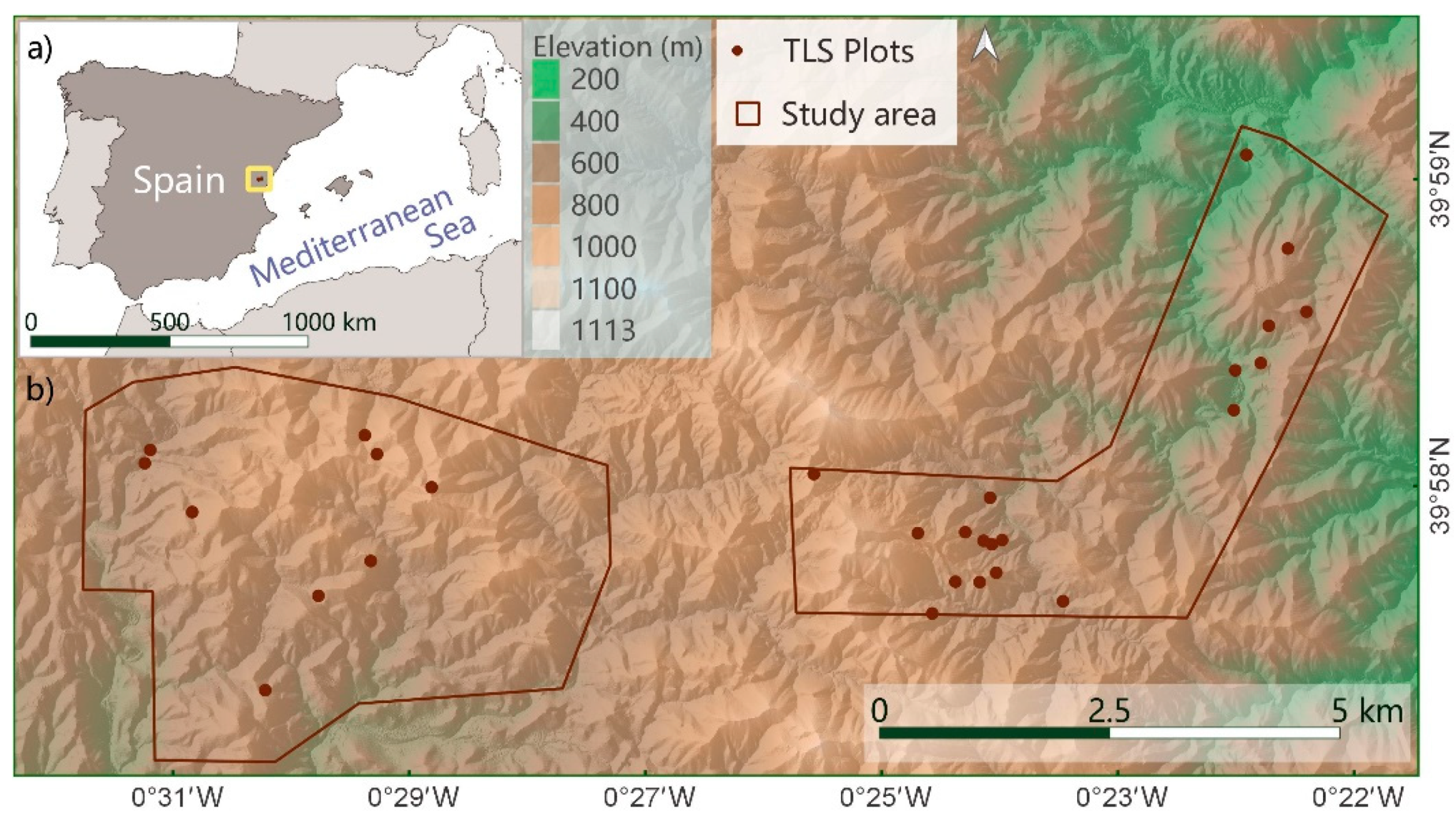
2.1. Study Area

The study area is located in the Natural Park of Sierra de Espadán on the eastern coast of the Iberian Peninsula (Castellón, Spain). This area is a Mediterranean mountainous forest with a natural function, composition, and structure, derived from complex historical interactions between anthropological impacts (i.e., farming terraces, wildfires, and reforestation) and harsh environmental conditions (i.e., severe drought and degraded soils) [19,30]. The plots were established in areas where trees have a uniform age structure, dominated by coniferous forests. The dominant tree species in the plots are Aleppo pine (Pinus halepensis Mill.) and maritime pine (Pinus pinaster Aiton), which are sometimes mixed with other deciduous species, such as cork oak (Quercus suber L.) and holm oak (Quercus ilex L.). The understory is made up of shade-tolerant Mediterranean species adapted to withstand the summer drought (e.g., Erica multiflora L., Genista Scorpius (L.) DC., Cistus sp. L., Pistacia lentiscus L., and Quercus coccifera L.), with an uneven distribution depending on the dominant tree species and the tree canopy cover.

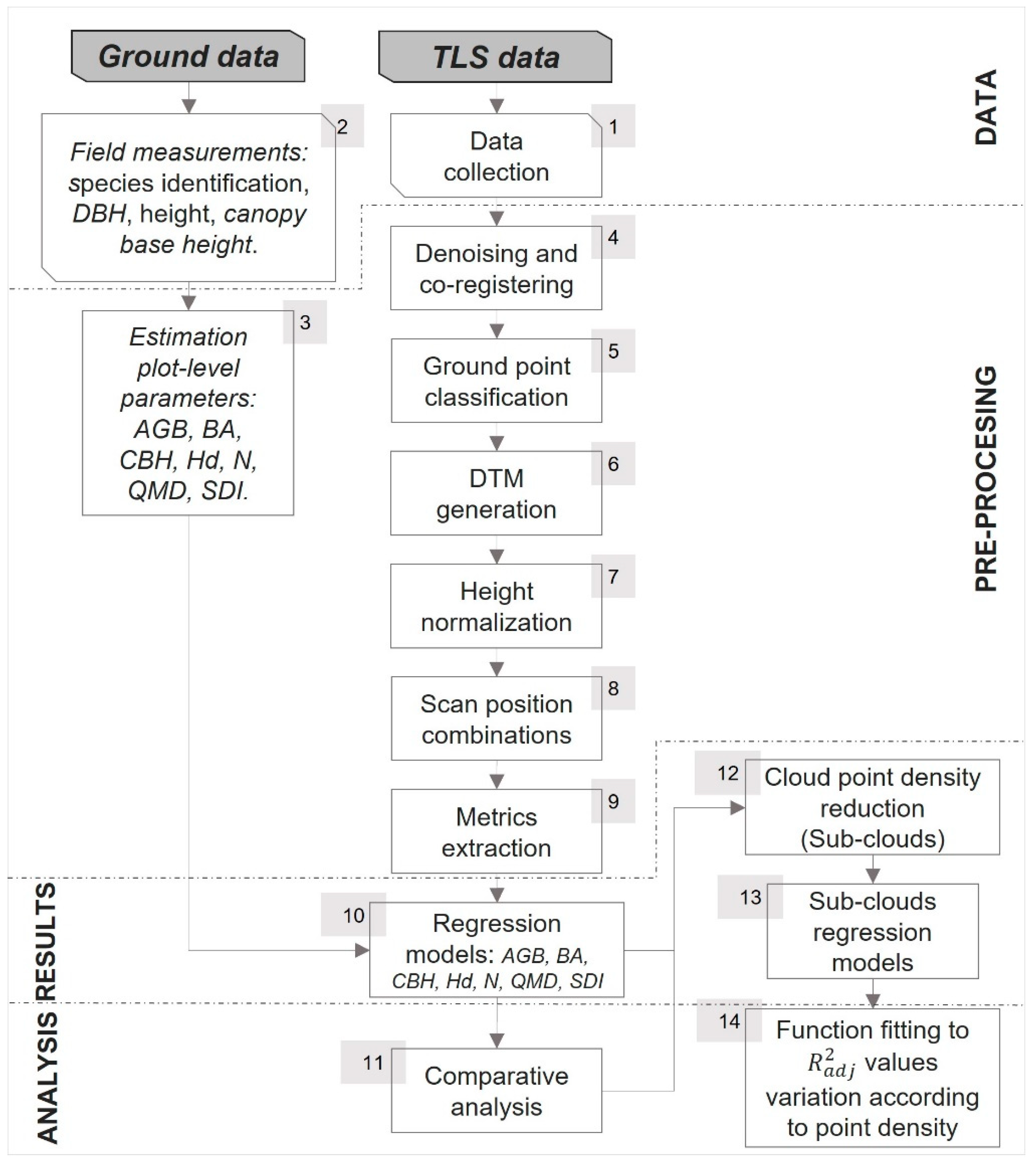
2.2. Methodology Overview

A general overview of the methodology and associated processes is illustrated in Figure 1. First, the TLS data were acquired in the field by setting six reference spheres at visible points, being at least three of them visible from each of the nine scan positions within the plot (step 1). After the point cloud acquisition, traditional forest inventory was carried out, characterizing the plot qualitatively and quantitatively (step 2). Tree ground truth data were processed to estimate the different parameters at the plot level (step 3). Simultaneously, all the point clouds were denoised and co-registered (step 4). Once the point clouds were co-registered, ground points were identified (step 5) and used to generate a digital terrain model (DTM) for each plot (step 6), and subsequently used to normalize the point cloud height (step 7). Afterwards, 31 combinations of different scan positions were created considering the location and distance of the scanner concerning the plot center (step 8). Then, for each of the 31-point cloud combinations, height metrics were extracted (step 9). Using the height metrics as independent variables and the forest parameters as dependent variables, we performed multiple linear regressions (step 10) with a subsequent assessment (step 11). Once the best model was identified for each forest parameter, we progressively reduced the point cloud density for the selected combinations (step 12). Finally, the weights of the independent variables were readjusted (step 13), and the influence of the reduction in point density on the estimation of the forest parameters was analyzed (step 14).

2.3. Field Data Collection

Data were acquired between September and October 2015 in 28 circular plots with a 15 m radius (i.e., 706 m2) (Figure 2). Plots were randomly distributed, avoiding inaccessible areas, to collect information on the different forest types (coniferous, broadleaves, and mixed) and different forest structures.

2.3.1. Reference Field Data

In each of the 28 plots, the diameter at breast height (DBH) and tree species were registered for all the trees with a DBH above 5 cm. The height and canopy base height were also measured for the seven trees with the greatest DBH (step 2 in Figure 1), following the criterion proposed by Assman [31], consisting of selecting the 100 dominant trees per hectare to estimate the height of the forest stand. Since our plots have an area of 706 m2, the proportional number of trees was seven. Additionally, terrain slope and herbaceous and shrub coverage per plot were measured. Afterwards, collected data were used to estimate forest parameters at plot level: AGB, BA, CBH, Hd, N, QMD, and SDI (step 3 in Figure 1). AGB was calculated per plot following the full tree allometric functions presented by Montero et al. [32] BA was obtained as the sum of the normal sections (at 1.30 m) of all the trees within the plot, then extrapolated to the hectare. CBH was calculated as the average of the canopy base height from the seven trees with the highest DBH per plot, Hd as the average of the height from the seven trees with the highest DBH per plot, and N as the number of trees within the plot. QMD represents the diameter of the tree of the average basal area in the stand [33]. SDI represents the density of the forest stands using the definition of Reineke [34], as an index based on the number of trees per hectare and the normal diameter of the mean basal area tree (i.e., the mean square diameter). The herbaceous cover is sparse, its and the maximum height varies from 0.15 to 0.30 m. The shrub cover is variable, with heights ranging from 0.41 to 1.07 m, with an average of 0.74 m. Table 1 summarizes the statistics for the 28 plots. In general, the 28 even-aged plots represent five different types of forest structures: (1) pure P. halepensis plots, pole wood, medium density (650–950 trees/ha); (2) pure P. halepensis plots, high forest, low density (350–600 trees/ha); (3) pure P. pinaster plots, pole wood, medium density (650–1100 trees/ha); (4) mixed plots of P. pinaster—Q. suber, different age classes, medium density (750–950 trees/ha); and, (5) mixed plots of P. halepensis—P. pinaster, different age classes, and medium density (600–700 trees/ha).

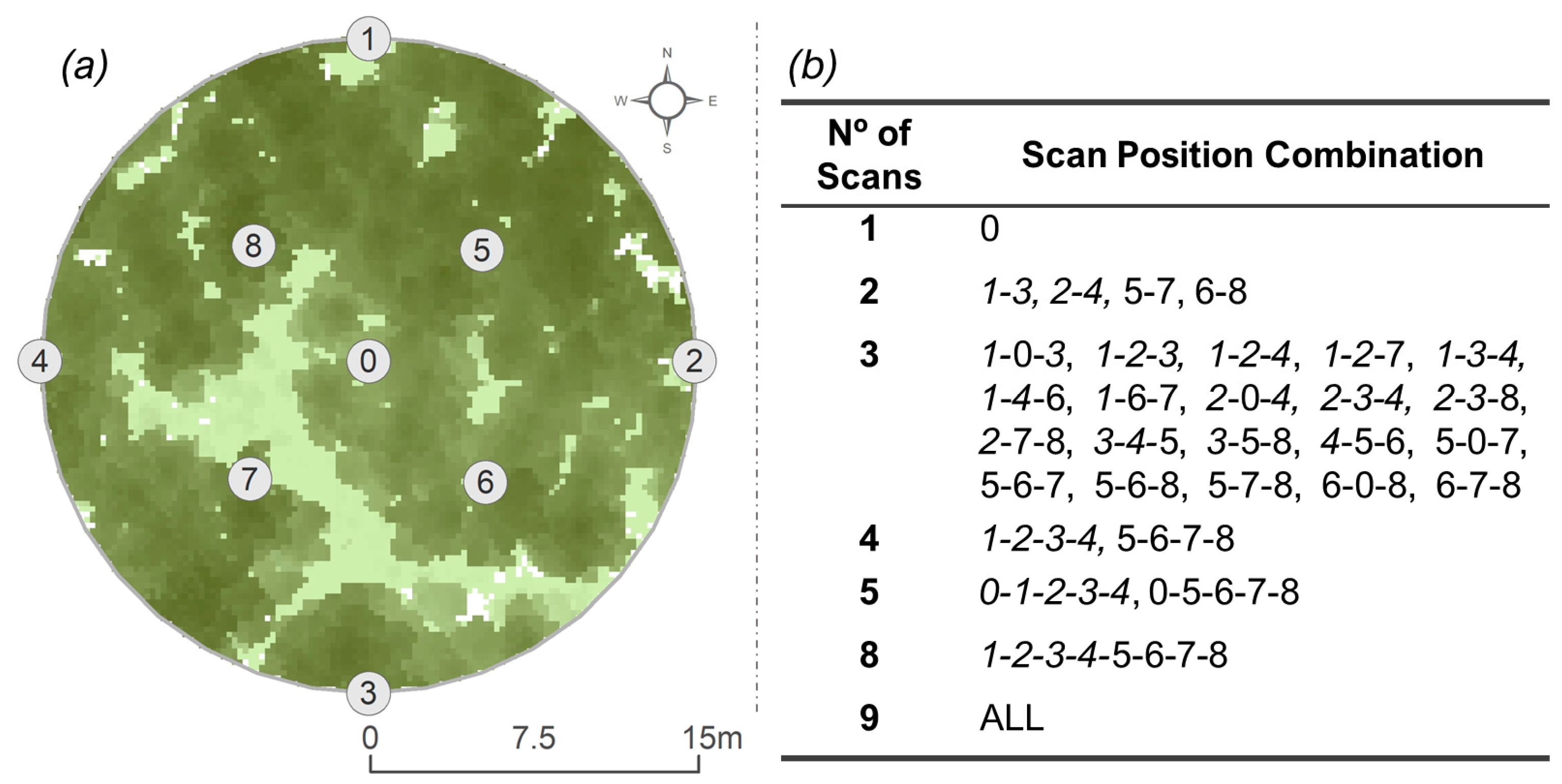
2.3.2. TLS Data Collection

TLS data acquisition (step 1 in Figure 1) was undertaken simultaneously with manual measurements of forest parameters using a FARO FOCUS 3D 120 (FARO Technologies Inc., Lake Mary, FL, USA) phase-based laser scanner whose technical specifications are shown in Table 2. TLS operated in 1/4 scan resolution mode and quality 2× (two sample points sent in the same direction to average the position of their returns); each scan took 1–3 min and produced a point cloud between 1800 and 23,700 points·m−2 (11,467.21 points · m−2 on average). Point density differences at each TLS position in the same plot were due to occlusion generated by the scanner position, differences in the forest structure, or the number of objects blocking the beam return to the sensor. For each return point, XYZ coordinates, intensity, plot id, and scan id were registered.
Data were collected on days without mist, fog, or rain with a wind speed below 5 m·s−1. Plot centers were measured using a Leica RTK 1200+ GPS (Leica Geosystems Inc., Heerbrugg, Switzerland) with an average XY dimension accuracy of 0.4 m ± 0.27 m, and 0.73 m ± 0.51 at the Z dimension. To minimize the occlusion and collect the forest structural variability of the plots, the sensor was placed in nine different positions per plot. A scan was established in the plot center, four acquisitions at 15 m (edge of the plot) in each cardinal direction (N, E, S, and W), and four acquisitions at 7.5 m in the secondary cardinal points (NE, SE, SW, and NW) (Figure 3a).

2.4. Data Pre-Processing

The nine TLS point clouds per plot were co-registered (step 4 in Figure 1) by identifying the different spherical targets (120 mm diameter) available in the point cloud in the FARO SCENE© software (Version 6.2, Lake Mary, FL, USA). To perform the co-registration, at least three spherical targets visible from adjacent scans were identified in each point cloud using a semi-supervised target-based approach. Co-registration accuracy in all plots was ±2 mm. Next, a supervised removal of anomalous points or noise was performed (step 4 in Figure 1).
To further retrieve normalized height metrics referred to the ground, it was firstly required to generate a DTM. To do this, ground points were identified (step 5 in Figure 1) by using the adaptation of the Axelsson [35] algorithm implemented in LAStools (Version 190114, Gilching, Germany) [36], selecting as input parameters an extra fine search for ground points in natural environments [37]. Next, points identified as ground were used to generate the DTM (step 6 in Figure 1). Then, the heights of all the point clouds were normalized (step 7 in Figure 1) using the DTM as the reference surface.
In order to perform the analysis of the distribution and number of TLS scans, the different point clouds registered from each position within each plot were combined as mentioned in Figure 3b.; i.e., from a single scan located in the plot center to the combination of the nine scans (step 8 in Figure 1). Nevertheless, the analysis of all possible combinations was discarded due to data processing volume (i.e., resulting in 9! combinations = 362,880). A total of 31 representative and geometrically balanced combinations were performed (Figure 3b.), trying to reflect the plot structure by covering the entire plot and minimizing the occlusion. The strategy followed to discard combinations was as follows: single scans were not used except for the scan at the center of the plot; for the combinations of two scan positions, the central scan was excluded, and the scans located at opposite sides with a distance of 7.5 m and 15 m from the center of the plot, were combined to increase the scanned area of the plot and maximize the information collected [38]; from the three-position combinations, the most representative and geometrically balanced combinations were selected, aiming to increase the area of the scanned plot and decrease the areas of low probability of detection [38]; with four scan positions, the main and secondary cardinal points were selected, excluding the central position and keeping a symmetric configuration; for five scan positions, the four previously mentioned positions were kept plus the central scan, following the same criteria; in the combination of eight scan positions, all the scans were included except the central one; and the last combination consisted of merging all the point clouds acquired in the plot. Tests combining six and seven scan positions were omitted because the symmetry and balance of the TLS positions, ensuring a homogeneous point distribution, would be lost.
The last TLS data pre-processing step consisted of obtaining a suite of height distribution metrics (Table 3) using the Fusion/LDV software (Version 3.8, Portland, OR, USA). [39] for each of the 31 scan combinations in the 28 plots (step 9 in Figure 1). To obtain these metrics, only points above 10 cm in height were considered, thus excluding the ground points and herbaceous vegetation. Intensity metrics were not included.

2.5. Regression Models

Forest parameters AGB, BA, CBH, Hd, N, QMD, and SDI were estimated at plot level applying ordinary multiple regression models (step 10 in Figure 1), using TLS height distribution metrics as independent variables. The Akaike information criterion (AIC) [40] was followed to reduce the number of TLS variables, which is a measurement of the adjustment of the relative model that expresses numerically the amount of information provided by each variable and statistically determines the number of parameters in an equation. Variables were selected consecutively until the AIC was minimized, thus obtaining a reduced set of predictive variables, with a maximum of three of them to avoid over-fitting.
Once variables were selected, stepwise multiple linear regression and the support vector machine (SVM) were applied to estimate the forest parameters, evaluating the models with the leave-one-out cross-validation technique (LOOCV). Finally, the resulting prediction models were analyzed by comparing the adjusted coefficient of determination (R2adj), RMSE, and the normalized RMSE (nRMSE), defined as the RMSE divided by the mean of the observed values (step 11 in Figure 1). The ordinary multiple linear regression model with the highest R2adj and the lowest RMSE was selected for each forest parameter to perform the point density reduction. Additionally, the influence of the terrain slope on the distribution and number of TLS scans was also evaluated. For this purpose, the set of plots was divided into two groups defined by the median value of the slope (22%) plots with a slight slope (i.e., <22%) and plots with a steep slope (i.e., >22%).

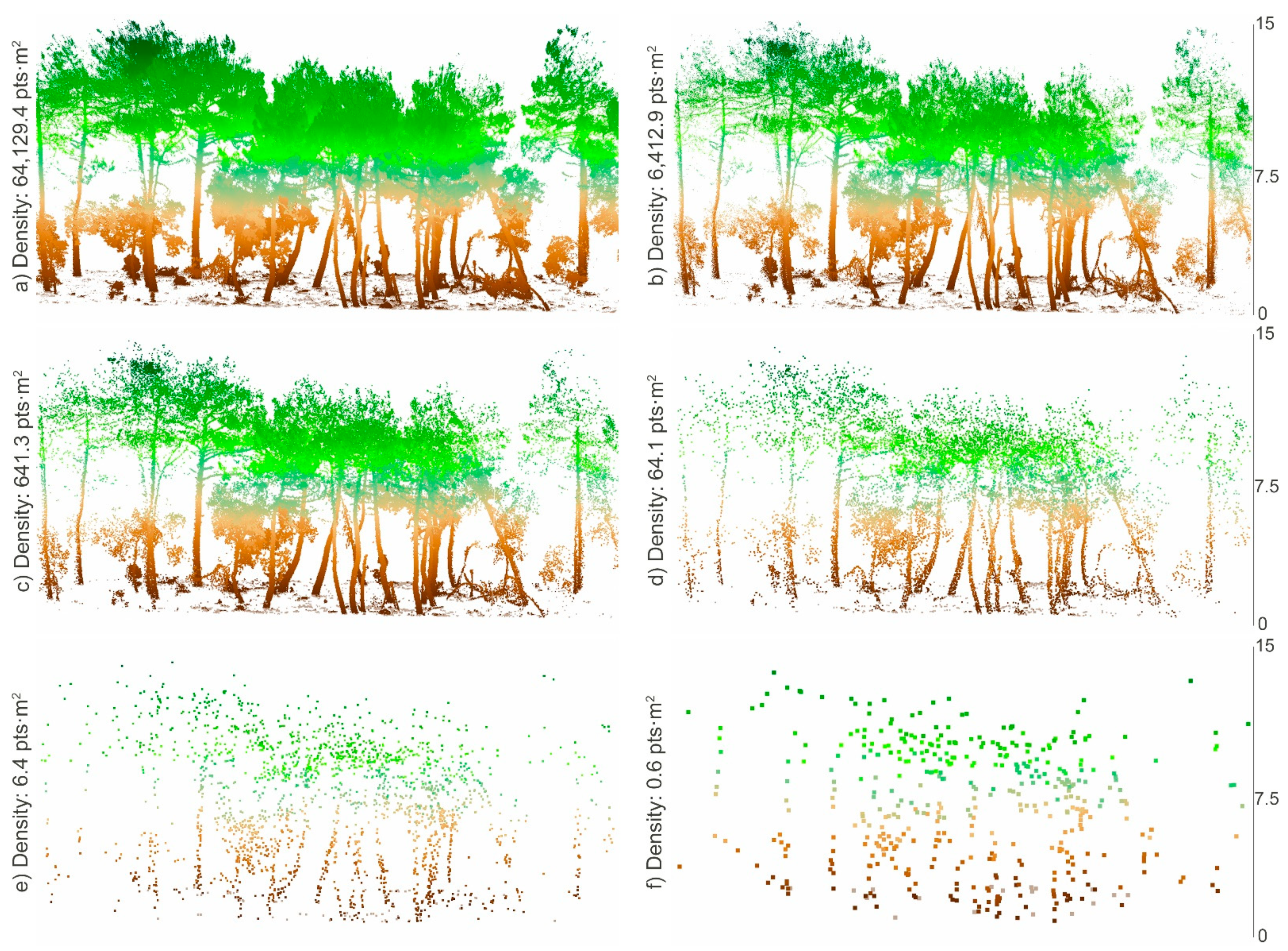
2.6. TLS Point Cloud Density Reduction

In order to test the influence of point density on the estimate of forest parameters, the number of points was decreased by random subsampling, implemented in the CloudCompare software (Version 2.11.3, Palaiseau, France) [41]. The random reduction applied is based on keeping randomly, in each plot, the number of points prefixed by the user with respect to the number of points present in the original point cloud. We performed progressive random point reduction from the initial point cloud (step 12 in Figure 1), where the point density for the seven selected combinations was between 4700 and 79,700 points·m−2. First, points were removed by intervals of 10% (10%, 20%, …, and 90%). After the deletion of 90% of points from the initial TLS point cloud, point density was reduced by intervals of 1% (91%, 92%, …,99%). When 99% of the points were eliminated, the density was reduced by intervals of 0.1% (99.1%, 99.2%, …, and 99.9%), then by intervals of 0.01% (99.91%, 99.92%, …, and 99.99%), then again by intervals of 0.001% (99.991%, 99.992%, …, and 99,999%), and finally by intervals of 0.0001%, resulting point clouds where 99.9991%, 99.9992%, …, and 99.9999% of the points from the initial point cloud were excluded. The reduction algorithm was always implemented from the original point cloud in order to maintain the randomness of the point selection, and not from the resulting point cloud obtained from a previous reduction. The random reduction process was repeated 10 times for each forest parameter to control the consistency of the results of the adjustment, independently of the points removed in each repetition.
As a result of the above description, for each forest parameter, a set of 54 sub-clouds with decreasing point densities was obtained. Figure 4 represents six profiles with a progressive reduction in the initial point density of plot number 28 with a mix of P. pinaster and Q. suber. From each sub-cloud, height distribution metrics were calculated (step 13 in Figure 1) following the procedure described in Section 2.4, to be used as potential independent variables in newly trained models created following the methods described in Section 2.5. Finally, the resulting models were evaluated by using R2adj, RMSE, and nRMSE, using LOOCV.
Once the evaluation was completed for every forest parameter and sub-cloud in each of the repetitions, we analyzed the variation in R2adj relative to each sub-cloud (step 14 in Figure 1). The variation in density was adjusted to a negative exponential distribution Equation (1), fitting a negative exponential model based on the exponential semivariogram model of David [42], and used by Crespo-Peremarch et al. [43] to model the influence of pulse density from full-waveform airborne laser scanning data on derived metrics. In this model, the values of R2adj (y = dependent variable) tend to remain stable until reaching a given point density (x = independent variable). The formula for the negative exponential function is the following:
y = a + c ( 1 e x p 3 x b )
where y = mean value of R2adj for the 10 repetitions by percentage reduction,
x =   value of density in points·m−2,
a = value of y where x = 0   in the negative exponential model,
b = value of x where y reaches 95% of the threshold value,
c = range of y, between a and the value of y, where the function is then stabilized,
a + c = y   value where the function stabilizes.

3. Results

3.1. Estimate of Forest Parameters Varying the Number and Distribution of TLS Scans

Regarding the relevance of the LiDAR height metrics used in the generation of the prediction models, the use of different metrics was observed for the 31 selected combinations in the estimate of the seven forest parameters. Figure 5 shows the percentage of use in the regression models for each LiDAR height metric. In general terms, it is observed that the most used elevation metrics were Elev. L. Kurtosis with 23.5%, followed by Elev. Skewness with 18.9%, and the percentiles of Elev. P75 and Elev. P70 with 18.4 and 17.5%, respectively, which were significantly used for AGB, BA, and SDI. The use of the metrics Elev. L. Kurtosis and Elev. L. Skewness in the models highlights the importance of abrupt changes in TLS point cloud height and point density distribution, which is consistent with interspecific differences between the vertical structure of P. halepensis plots (where first branches are above 1.1 m) and P. pinaster plots (where first branches are above 5.5 m). The remaining metrics were used 15% or less, where the most relevant metrics for the other parameters were Hd, Elev. P60, Elev. L. Skewness and Elev. L4; for N, the Elev. SD, the Elev. Kurtosis and the IQ; for QMD, the Elev. Variance, the Elev. MAD. Mode and Elev. SQRT mean SQ; and for CBH, the % ARA-mean, the Elev. SQRT mean SQ and the Elev. L. Kurtosis. The selected metrics reflected the complementarity of two groups of metrics (forest height metrics and forest height variability metrics) to describe and explain five parameters (AGB, BA, SDI, Hd and QMD) and the influence of the forest density metrics in explaining the CBH parameter. Testing the results obtained with the ordinary multiple linear regression and SVM, the same TLS optimal combinations were obtained for all the forest parameters using both methods. Nevertheless, on the grounds that the number of samples, determined by the number of plots, was limited, and due to the risk of over-fitting and the complexity of application if using the SVM model, only the multiple linear regression was performed.
Figure 6 shows the variation in the adjusted R2 resulting from the estimate of each forest parameter and each of the 31 combinations of scan number and position, for all the 28 plots (white boxes) and the plots divided according to their terrain slope (light and dark brown boxes). When using all the plots, the CBH parameter was the least susceptible to variations in the number and positions of TLS scans, with an R2adj interquartile range of 10%. For BA and SDI parameters, the interquartile range of the R2adj obtained was about 20%, and for AGB, QMD, Hd, and N parameters, the variation in the position and number of the TLS scans resulted in 30% of the interquartile range in the R2adj of the models. There were also differences in the distribution of the R2adj result adjusted by the parameter: for AGB and SDI, about 50% of the models were above an R2adj of 0.8 whose distribution was negatively skewed; AGB had 50% of the models above an R2adj of 0.75 with a normal distribution with a tendency to be negatively skewed; CBH followed a normal distribution with a median being close to an R2adj of 0.8; Hd had a normal distribution with a tendency to be negatively skewed, with a median value of R2adj equal to 0.7, and an extreme maximum value; for QMD, all of the models were below an R2adj of 0.6 with a nearly symmetrical distribution; and for the N parameter, the best model achieved an R2adj equal to 0.628, but half of the models had an R2adj lower than 0.35. Considering the terrain slope (Figure 6), it was observed that in slight slopes, mean accuracy of the observations was improved by 10%, 9%, 5%, and 1% for the forest parameters AGB, BA, SDI, and CBH with respect to steep slopes. In contrast, in steep slopes mean accuracy was improved by 2%, 20%, and 40% for the forest parameters Hd, N, and QMD. It was also observed that the differences in accuracies of the selected models for both slope classes were lower than 5% for CBH, Hd, and SDI forest parameters, and increased above 10% for the AGB, BA, N, and QMD forest parameters.
Following results obtained for all the plots shown in Figure 6, Table 4 represents in detail the results of the estimate of forest parameters related to the position in the plot and the number of TLS scans. This table shows the combination of scans with the highest R2adj for each forest parameter, which was selected for the point density reduction and analysis; as well as the results obtained for the central scan (0) and the nine-scan combination (ALL). The table also shows the mean, maximum, and minimum values obtained for R2adj, RMSE, and nRMSE. It is observed that, regardless of the forest parameter, estimation accuracies ranged from 60% to 85% using five, three, or one scan. For AGB, BA, Hd, and N, the resulting values of R2adj for the selected combination improved by more than 10% (12.8, 11.2, 11.8, and 26.5%, respectively) compared to only using the central scan. On the other hand, using the selected combination improved the R2adj above 10% compared to using the nine scans for the Hd (14.3%) and N (28.5%), resulting in a lower improvement for the rest of the forest parameters. However, in all the cases, the selected combination improved the R2adj compared to the average value. In addition, it was observed that combinations of five scans including the central scan and the four interior positions at 7.5 m (Table 4 and Figure 3a) provided better results for the AGB and BA. For the Hd and SDI parameters, the best results were obtained with three scans including one interior position at 7.5 m and two external scans at 15 m, and for CBH, the best results were obtained with the central and two internal scans at 7.5 m. Furthermore, the combination selected decreased the RMSE in the prediction of all the forest parameters with respect to the use of a single scan or nine scans. In comparison with the estimate obtained from a single scan, the parameters that most reduced the RMSE by using the selected combination of scans were AGB (0.5 t·plot−1), BA (1.7 m2·ha−1), Hd (0.3 m), N (2.9 trees·plot−1), and SDI (21.1 trees·ha−1). On the other hand, the RMSE decreased by using the selected combination concerning using the nine scans for forest parameters AGB (0.1 t·plot−1), BA (0.7 m2·ha−1), SDI (9.8 trees·ha−1), Hd (0.4 m), and N (3.0 trees·plot−1). Comparing the use of nine and a single scan, the RMSE in the estimate of AGB, BA, and SDI was reduced when using nine scans, while the RMSE in the estimate of Hd and N was reduced when using a single scan. In all cases, the nRMSE was below 10% except for N and QMD, which achieved 16% and 14%, respectively.
On the other hand, for the analysis of combinations according to their terrain slope, the selected combinations differed from those selected when using all the plots. Figure 7 shows that in all cases, except for the CBH in slight slope, the selected combination improved the accuracy with respect to the use of all the scans. Using only the central scan, it was observed that lower accuracies were obtained, regardless of the slope class. The central scan was only relevant in the model selected for CBH on a steep slope. In the models selected for slight slope, scans at 7.5 m predominated for AGB, BA, Hd, and QMD, and in the models for steep slope, scans at 15 m and 7.5 m were combined for AGB, BA, CBH, Hd, and QMD parameters.
Focusing on the use of the selected multiple linear regression models having the highest R2adj values, Figure 8 shows the scatterplot of predicted and observed values of the seven forest parameters (AGB, BA, CBH, Hd, N, QMD, and SDI). The most accurate estimations, with an R2adj close to 0.9, were obtained for AGB, BA, CBH, Hd, and SDI forest parameters, also reaching a low RMSE (e.g., 0.8 m for Hd, 0.7 m for CBH). On the contrary, the least accurate estimations were obtained for N and QMD, where the R2adj values were below 0.75, and the RMSE were equal to 7.31 trees·plot−1 and 2.11 cm for N and QMD, respectively. In addition, the results of the equivalence test for these forest parameters show that they are statistically equivalent in terms of bias.

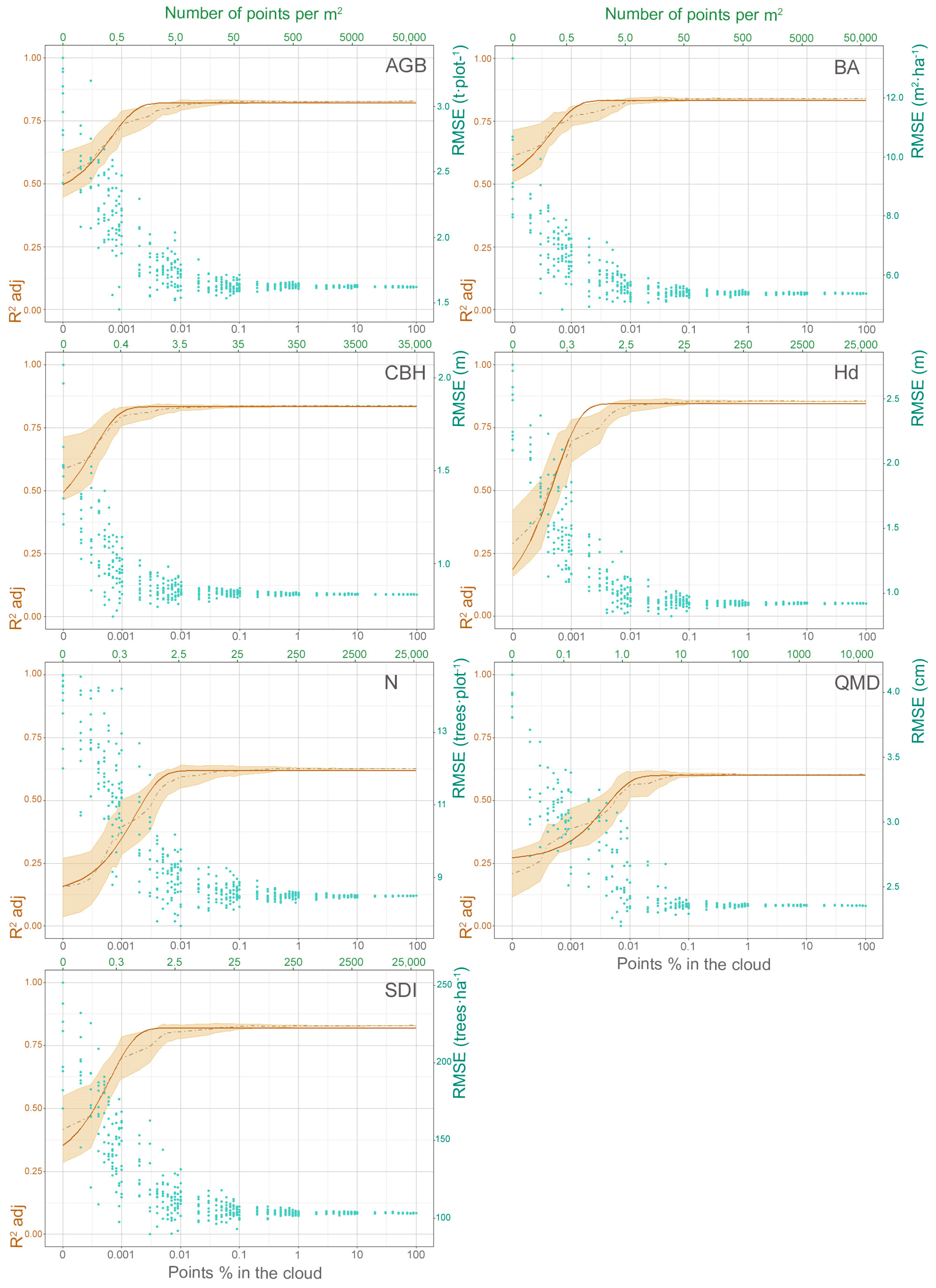
3.2. Analysis of the TLS Point Cloud Density Reduction

Figure 9 shows the variation in R2adj and RMSE in estimating the forest parameters with different point cloud densities, reducing from the initial density (4783–79,689 points·m−2) to a percentage of 0.0001% (0.01–1 points·m−2). On the Y-axis of the graphs, the area of the R2adj values obtained for the 10 test repetitions for each percentage of points is plotted in light brown. The brown line represents the negative exponential function that fits the mean of the 10 test repetitions in each percentage reduction step, having R2 values of 0.82 for AGB, 0.73 for BA, 0.72 for CBH, 0.84 for Hd, 0.85 for N, 0.79 for QMD, and 0.82 for SDI. For all the forest parameters studied, the trend fits the negative exponential model, where it is observed that the reliability of the predictions starts to decrease when the point density is reduced between 1/10,000 and 1/100,000 with respect to the original density. In particular, the statistic R2adj drops below 0.75 when analyzing 0.008% (2–6 points·m−2) for AGB, 0.005% for BA (1–4 points·m−2), 0.001% for CBH (0.2–0.5 points·m−2), 0.007% (1–3 points·m−2) for Hd, and 0.01% (1–5 points·m−2) for SDI compared to the initial point density. This is not the case for the QMD and N parameters, where the models do not exceed an R2adj of 0.65. On the other hand, the RMSE increases with the decreasing point density. For the forest parameters AGB, Hd, N, QMD, and SDI, it can be observed that the dispersion of the RMSE values for each point density increases when the point density is below 0.1% (13 to 61 points·m−2, depending on the forest parameter), although the trend of the negative exponential curve is preserved. This result suggests that, although the R2adj remains at high values, the goodness of fit is lower above this point density. On the other hand, the dispersion of the RMSE values in the BA and CBH forest parameters increases when the point density drops below 0.01%, being the goodness of fit valid up to this point density (4 to 6 points·m−2).

4. Discussion

In this research, we analyzed how the accuracy in estimating seven forest parameters at stand level using height metrics extracted from TLS point clouds varied according to (1) the number and distribution of TLS scans, and (2) the point density. Key results indicate that considering a standard plot size for forest inventories, the use of three to five scans is optimal, and it is not necessary to use more. In addition to the number of scans, it was observed that the use of specific scan distributions for each forest parameter improves the results. Concerning terrain slope, higher accuracies are usually obtained in slight slopes as compared to the ones obtained in steep slopes. High-density TLS point clouds were shown to be redundant to estimate forest parameters based on height metrics.
Results show that there is a particular number of TLS scans, regardless of the forest parameter studied, that optimize the accuracy. It is logical to assume limitations in capturing information due to the occlusion generated by surrounding trees and shrubs. This suggests that conducting a larger number of scans increases the chances of capturing all target objects within an intended sample area [3,4,44]. In this sense, it was observed that those parameters based on tree diameters, such as AGB and BA, were optimized using five positions, and those dependent on height measurements, such as CBH and Hd, only needed three positions (Table 4). An exception was SDI, which, despite being based on the allometric relationship of the number of trees per hectare as a function of the root mean square diameter, required only three positions. Another exception was that the QMD parameter was optimized using only the central position; however, its weak accuracy of 60% (Table 4) limits the extraction of explicit conclusions. In terms of accuracy, the number of positions selected improved the prediction accuracy with respect to using only the central scan by 6–27%. Our results are in agreement with Hilker et al. [45], Lovell et al. [24], and Wilkes et al. [4], who indicated that a single scan location could be affected by a limited sampling of the forest canopy and occlusion of distant vegetation by foreground objects; therefore, a systematic approach of multiple scan locations and subsequent joint registration would be desirable in practice. However, there are significant differences in the data collection performed in these three studies. Hilker et al. [45] compared the height determination with TLS and ALS in a coniferous forest, using a central scan and four scans at 30 m. Lovell et al. [24] estimated a DBH-derived basal area in a P. ponderosa plantation, analyzing the decrease in DBH accuracy as the surveyed object was moved further away from the sensor in 20 m plots with a single scan. Wilkes et al. [4] conducted 24 field campaigns in different forest types (mainly tropical rainforests) and proposed methods for estimating individual trees and large areas. The individuals were recorded with six scans, while for large areas they proposed a grid of scans with a separation of 10 m to generate a homogeneous point cloud. Forest data capture methodologies with TLS were different from each other. Results obtained in this current study show that the accuracy improves between 1% and 14% when using the optimal scan positions with respect to using all positions (nine scans). This has a practical application in terms of time and cost reduction in field inventories. This effect of the useless increase in scan locations was also noticed by Boucher et al. [44], who demonstrated with geometric models for stem estimation in forest plots that even the plots sampled with the highest number of scans cannot guarantee a complete sample if the positions of the TLS scans are based on a predetermined layout. Therefore, in practice, determining the optimal number of positions can optimize the time for acquisition and processing of the collected data volume, considering that forest parameters based on the DBH, such as AGB or BA, will need more scans than parameters only referring to height measurements, such as Hd and CBH.
On the other hand, results show that for each forest parameter there is an optimal distribution of scans. For parameters based on tree width, such as AGB and BA, it was observed that the central scan and four scans at 7.5 m were optimal, i.e., the TLS needed to collect data from the inner part of the plot. Likewise, the CBH parameter was optimized with the central position and two positions at 7.5 m in order to collect information from the lower part of the canopy. This selection of positions is particularly relevant in Mediterranean forest plots such as those used in this study, dominated by P. halepensis, with average CBH of 5.85 m and minimum height of 1.1 m (Table 1), and plots of P. pinaster, where the CBH was 8.30 m. In contrast, the Hd parameter was optimized with one position at 7.5 m and two positions at the plot edge (i.e., 15 m), probably due to the need to increase the distance from the TLS to the trees to properly capture the height of the trees. This is in agreement with the findings of Martins Neto et al. [46], who analyzed the TLS scanning distance (5 m, 10 m, 15 m, and 20 m) influence on measuring diameters and heights of sample trees, and concluded that the optimal scanning distance is related to the height of trees, where the best scanning distance to obtain reliable parameters was 15 m and distances less than 10 m were not recommended. The N and SDI parameters required at least two scans at the plot edge (15 m), with one more scan at 15 m for N and at 7.5 m for SDI. This similarity in distribution also showed the relationship between the two parameters. Regarding the error obtained in each parameter, the combination of scans 0-5-6-7-8 for AGB obtained an error of 1.61 t·ha−1, which was below the one presented by other authors [10] who used the same methodology, but in tropical environments. For BA (scan combination 0-5-6-7-8) the error obtained was 5.35 m2·ha−1, improving those obtained by Molina-Valero et al. [47], with an RMSE of 8.57 m2·ha−1 for pure plots of P. sylvestris L. with a radius of 7 m and performing a single TLS measurement from the plot center. The error obtained in the estimation of the CBH with the combination of three scans (5-0-7) was 0.83 m lower than 1.95 m obtained by Giannetti et al. [48] in the CBH study performed on a set of individual trees of Cupressus sempervirens L. and P. pinaster with eight scanner positions. Despite the well-known difficulty of TLS to reach the top of the tree canopy, the error in height estimation was between 0.9 and 1.6 m, which is lower than the error reported in other studies also using multiple scan in boreal and temperate forests, where the Hd was bounded between 16.1 and 31.4 m, and the RMSE between 1.9 and 6.5 m [49,50,51,52]. This lower error in the Hd probably occurred because our study area was dominated by P. pinaster and P. halepensis, with a canopy shape and low density allowing the sensor beams to reach the top of the trees. For the N and QMD forest parameters, the optimal combinations were not accurate (R2adj < 0.65), with an error of 8.45 trees·plot−1 and 2.35 cm, respectively. Considering these results for N and QMD, it is suggested to use other approaches for processing TLS data where stem locations are detected and DBH is calculated directly on the point cloud, following geometric modeling methodologies, such as those implemented by Gollob et al. [20] or by Molina-Valero et al. [21]. The optimal model for estimating the SDI had an RMSE of 101.94 trees·ha−1. Results for SDI are promising, since they allow measuring the stocking density of the forest stand. However, in order to compare the degree of space available for trees of different ages and season quality in the plots, it would be necessary to establish the reference stand, usually defined with maximum competition or non-competition [53]. Notwithstanding the results obtained, it should be clarified that the specific distribution of the scanner for each parameter is conditioned by the vertical and horizontal structure of the vegetation in each plot. The TLS registration of Mediterranean vegetation is a logistical challenge and, in some cases, constructing a 3D mosaic of the entire plot is unfeasible or requires modifying the layout of the scans in situ to minimize the occlusion generated by the surrounding vegetation. Modifications to the data acquisition design during TLS registration were also studied by Abegg et al. [54], recommending in their study the use of an intuitive distribution of TLS positions uniformly within the sampling plot to obtain the best overall plot visibility. However, if the interest involves studying the evolution of vegetation over time, as in forest inventories, it is advisable to adopt a minimum data standard and a TLS data acquisition protocol to ensure data comparability between different campaigns.
The analysis considering the terrain slope showed that it influences the selection of the best combination to predict forest parameters. In general, the accuracies for the different combinations increase when considering the terrain slope rather than using all the 28 plots (Figure 6). Specifically, for slight slope terrains, accuracies were improved for AGB by 10%, BA by 9%, CBH by 8%, Hd by 5%, and SDI by 8%, compared to using all the plots. Figure 7 shows that for forest parameters AGB, BA, CBH, Hd, and SDI, the highest accuracies were obtained for slight slopes. For both terrain slope classes, it was observed that combinations of three scans improved the accuracy with respect to the use of the central and nine scans. Most of the selected positions in the combinations on slight slope plots were located inside the plot at 7.5 m from the center, while on steep slope plots, at least one TLS position was located at the edge of the plot at 15 m, which could indicate that steeper slopes require larger spacing between scans to record the plot characteristics. Most studies that estimated structural forest parameters using TLS used data were located in flat areas [18,29], did not perform any comparative study with different slope ranges [28,55], or found no significant effects on the forest parameter estimations [20]. Although this study did analyze the influence of terrain slope, the results should be considered preliminary, since a larger set of plots should be studied, stratified in different slope ranges.
The analysis performed with point density reduction indicated that high point densities are not necessary for the estimation of forest parameters with height metrics extracted from TLS point clouds. Ruiz et al. [56] obtained parallel results in a study conducted with ALS point clouds, also in a Mediterranean area, concluding that a minimum point density was necessary, but increasing it does not guarantee the improvement of the prediction of forest parameters. Kankare et al. [57], with a manual approach for tree detection and DBH measurement, concurred that point cloud subsampling can be used effectively without losing accuracy in tree detection. However, when measuring the attributes of a single tree, they recommend using the complete point cloud data. Litkey et al. [58] indicated that longer-range stem data can be observed with point cloud reduction if the data reduction scheme is carefully selected. These authors also concluded that a significant reduction in point cloud size allows multi-scan studies for being more manageable while retaining their inherent accuracy [58]. Figure 9 shows that the variations of accuracy related to point density follow a negative exponential behavior, especially when the density is below 6.4–0.2 points·m−2. Generally, there is a density above, which the accuracy stabilizes in the parameters AGB, BA, CBH, Hd, N, and SDI. However, when the percentage of points is less than 0.1% of the original cloud points, the variability of the RMSE is extremely high (Figure 9), so it is advisable not to reduce the cloud below 60–65 points·m2 for the parameters AGB and BA, nor below 38, 30, and 13 points·m2 for CBH, Hd, and QMD parameters, respectively. For the N and SDI parameters, it was shown that working with 1% of the point cloud allowed for a lower error variability, i.e., reducing the point cloud to densities of 271 and 309 points·m−2, respectively. In summary, lower point densities can be used, and this is consistent with the results mentioned above, since allocating the TLS in strategic positions and with the appropriate number of scanners can reduce the density and even reduce the pulse frequency, optimizing acquisition time and costs, processing time, and hardware requirements. Although in our site conditions optimal results were obtained working with point clouds with densities between 13 and 309 points·m−2 of the original point cloud density, it is expected that in denser forest environments, such as tropical forests, with higher and denser canopy, the reduction in the number of points should be lower.
The use of a reduced number of TLS scans in a strategic distribution and with a low density of points allowed us to obtain high accuracy in the estimation of forest parameters. In this work, we showed a methodology that provides a faster, less costly, and less time-consuming forest inventory for three reasons. Firstly, a minimum number between three to five TLS scans should be set to ensure that the prediction of all forest parameters is optimized. Secondly, there are strategic positions for each forest parameter, so depending on the objective and terrain slope, some positions or a combination of several strategies should be considered to collect information for all the forest parameters. If the intention is to compare the forest inventory over time and by different users, it is appropriate to maintain an acquisition strategy. Finally, the density of points in the TLS point cloud can be deeply decreased without loss of accuracy, thus the minimum pulse rate of the sensor can be reduced and lower resolution scanners could be used, such as the case of new MLS that are already available in the last few years. The use of height metrics derived from TLS point clouds proved to be accurate and useful, considering the processing simplicity. These findings allow us to optimize the field acquisition of the forest inventory in a more accurate approach than traditional techniques.

5. Conclusions

The present study analyzed the influence of the number and distribution of TLS scans on the estimate of forest parameters at stand level based on models derived from height metrics by considering the terrain slope and the point density. Our results suggest that the optimal number of scans ranges from three to five. Using only one scan reduces the accuracy of the models between 0.06 and 0.27, depending on the forest parameter, and using nine scans also reduces the accuracy between 0.01 and 0.29. The configuration of one scan in the plot center and the others equidistant to the limit of the plot is the most adequate in practically all the parameters assessed. Regarding terrain slope, our results suggest that steep slopes decrease the accuracy in estimating forest parameters with respect to slight slopes. The use of interior scans is sufficient for slight terrain slopes, but for steep terrain slopes, it is convenient to combine scans inside and outside the plot. In terms of point density, using 1% to 0.1% of the initial density, which is equivalent to reducing the absolute density on average from 37,240.86 to 136 points·m−2, generates an R2adj difference of less than 0.01 compared to using 100% of the initial cloud point density; and a maximum difference in RMSE of only 0.12 t·plot−1, 0.14 m2·ha−1, 0.02 m, 0.03 m, 0.03 cm, and 3.07 trees·ha−1 for AGB, BA, CBH, Hd, QMD, and SDI, respectively. These results are based on tests performed in a Mediterranean forest with mixed tree and shrub species and could be subject to variation in other areas as a function of the density and height of the vegetation (e.g., tropical forests). However, results are particularly relevant for forest management since they prove the suitability of TLS data for forest inventories and provide practical criteria to optimize the acquisition and processing times and cost of TLS data. Since a considerable reduction in pulse density seems not to affect the accuracy of the prediction models in the forest parameters assessed, further comparative analysis can be focused on the use of MLS with lower scan frequencies than TLS.

Author Contributions

J.T. and L.Á.R. conceptualized the paper; J.T., J.P.C.-R., L.Á.R. and P.C.-P. performed the data collection; J.T. and L.Á.R. developed the methodology; J.T., J.P.C.-R. and P.C.-P. developed the software and performed the formal analysis; J.T. and J.P.C.-R. wrote the manuscript; L.Á.R. and P.C.-P. revised the manuscript; L.Á.R. supervised and acquired the funding. All authors have read and agreed to the published version of the manuscript.

Funding

This research has been funded by the project PID2020-117808RB-C21 MCIN/AEI/10.13039/501100011033 and by the grant PEJ2018-002924-A Fondo de Garantía Juvenil en I+D+i ESF Investing in your future.

Data Availability Statement

The data presented in this study are available on request from the corresponding author (J.T.).

Acknowledgments

The authors would like to thank Jaime Almonacid-Caballer for his constructive comments and suggestions that improved the quality of this work.

Conflicts of Interest

The authors declare no conflict of interest.

References

  1. Tinkham, W.T.; Mahoney, P.R.; Hudak, A.T.; Domke, G.M.; Falkowski, M.J.; Woodall, C.W.; Smith, A.M.S. Applications of the United States Forest Inventory and Analysis Dataset: A Review and Future Directions. Can. J. For. Res. 2018, 48, 1251–1268. [Google Scholar] [CrossRef]
  2. Lister, A.J.; Andersen, H.; Frescino, T.; Gatziolis, D.; Healey, S.; Heath, L.S.; Liknes, G.C.; McRoberts, R.; Moisen, G.G.; Nelson, M.; et al. Use of Remote Sensing Data to Improve the Efficiency of National Forest Inventories: A Case Study from the United States National Forest Inventory. Forests 2020, 11, 1364. [Google Scholar] [CrossRef]
  3. Newnham, G.J.; Armston, J.D.; Calders, K.; Disney, M.I.; Lovell, J.L.; Schaaf, C.B.; Strahler, A.H.; Mark Danson, F. Terrestrial Laser Scanning for Plot-Scale Forest Measurement. Curr. For. Rep. 2015, 1, 239–251. [Google Scholar] [CrossRef] [Green Version]
  4. Wilkes, P.; Lau, A.; Disney, M.; Calders, K.; Burt, A.; Gonzalez de Tanago, J.; Bartholomeus, H.; Brede, B.; Herold, M. Data Acquisition Considerations for Terrestrial Laser Scanning of Forest Plots. Remote Sens. Environ. 2017, 196, 140–153. [Google Scholar] [CrossRef]
  5. LaRue, E.A.; Wagner, F.W.; Fei, S.; Atkins, J.W.; Fahey, R.T.; Gough, C.M.; Hardiman, B.S. Compatibility of Aerial and Terrestrial LiDAR for Quantifying Forest Structural Diversity. Remote Sens. 2020, 12, 1407. [Google Scholar] [CrossRef]
  6. Liang, X.; Kankare, V.; Hyyppä, J.; Wang, Y.; Kukko, A.; Haggrén, H.; Yu, X.; Kaartinen, H.; Jaakkola, A.; Guan, F.; et al. Terrestrial Laser Scanning in Forest Inventories. ISPRS J. Photogramm. Remote Sens. 2016, 115, 63–77. [Google Scholar] [CrossRef]
  7. Liang, X.; Hyyppä, J.; Kaartinen, H.; Lehtomäki, M.; Pyörälä, J.; Pfeifer, N.; Holopainen, M.; Brolly, G.; Francesco, P.; Hackenberg, J.; et al. International Benchmarking of Terrestrial Laser Scanning Approaches for Forest Inventories. ISPRS J. Photogramm. Remote Sens. 2018, 144, 137–179. [Google Scholar] [CrossRef]
  8. Bauwens, S.; Bartholomeus, H.; Calders, K.; Lejeune, P. Forest Inventory with Terrestrial LiDAR: A Comparison of Static and Hand-Held Mobile Laser Scanning. Forests 2016, 7, 127. [Google Scholar] [CrossRef] [Green Version]
  9. Liang, X.; Kukko, A.; Kaartinen, H.; Hyyppä, J.; Yu, X.; Jaakkola, A.; Wang, Y. Possibilities of a Personal Laser Scanning System for Forest Mapping and Ecosystem Services. Sensors 2014, 14, 1228–1248. [Google Scholar] [CrossRef]
  10. Zimbres, B.; Shimbo, J.; Bustamante, M.; Levick, S.; Miranda, S.; Roitman, I.; Silvério, D.; Gomes, L.; Fagg, C.; Alencar, A. Savanna Vegetation Structure in the Brazilian Cerrado Allows for the Accurate Estimation of Aboveground Biomass Using Terrestrial Laser Scanning. For. Ecol. Manage. 2020, 458, 117798. [Google Scholar] [CrossRef]
  11. Crespo-Peremarch, P.; Fournier, R.A.; Nguyen, V.; van Lier, O.R.; Ruiz, L.Á. A Comparative Assessment of the Vertical Distribution of Forest Components Using Full-Waveform Airborne, Discrete Airborne and Discrete Terrestrial Laser Scanning Data. For. Ecol. Manage. 2020, 473, 118268. [Google Scholar] [CrossRef]
  12. Danson, F.M.; Hetherington, D.; Morsdorf, F.; Koetz, B.; Allgower, B. Forest Canopy Gap Fraction From Terrestrial Laser Scanning. IEEE Geosci. Remote Sens. Lett. 2007, 4, 157–160. [Google Scholar] [CrossRef] [Green Version]
  13. Lovell, J.L.; Jupp, D.L.B.; Culvenor, D.S.; Coops, N.C. Using Airborne and Ground-Based Ranging Lidar to Measure Canopy Structure in Australian Forests. Can. J. Remote Sens. 2003, 29, 607–622. [Google Scholar] [CrossRef]
  14. Calders, K.; Adams, J.; Armston, J.; Bartholomeus, H.; Bauwens, S.; Bentley, L.P.; Chave, J.; Danson, F.M.; Demol, M.; Disney, M.; et al. Terrestrial Laser Scanning in Forest Ecology: Expanding the Horizon. Remote Sens. Environ. 2020, 251, 112102. [Google Scholar] [CrossRef]
  15. Domingo, D.; Lamelas, M.; Montealegre, A.; García-Martín, A.; de la Riva, J. Estimation of Total Biomass in Aleppo Pine Forest Stands Applying Parametric and Nonparametric Methods to Low-Density Airborne Laser Scanning Data. Forests 2018, 9, 158. [Google Scholar] [CrossRef] [Green Version]
  16. van Leeuwen, M.; Nieuwenhuis, M. Retrieval of Forest Structural Parameters Using LiDAR Remote Sensing. Eur. J. For. Res. 2010, 129, 749–770. [Google Scholar] [CrossRef]
  17. White, J.C.; Coops, N.C.; Wulder, M.A.; Vastaranta, M.; Hilker, T.; Tompalski, P. Remote Sensing Technologies for Enhancing Forest Inventories: A Review. Can. J. Remote Sens. 2016, 42, 619–641. [Google Scholar] [CrossRef] [Green Version]
  18. Srinivasan, S.; Popescu, S.C.; Eriksson, M.; Sheridan, R.D.; Ku, N.W. Multi-Temporal Terrestrial Laser Scanning for Modeling Tree Biomass Change. For. Ecol. Manage. 2014, 318, 304–317. [Google Scholar] [CrossRef]
  19. Torralba, J.; Crespo-Peremarch, P.; Ruiz, L.Á. Assessing the Use of Discrete, Full-Waveform LiDAR and TLS to Classify Mediterranean Forest Species Composition. Rev. Teledetección 2018, 52, 27. [Google Scholar] [CrossRef] [Green Version]
  20. Gollob, C.; Ritter, T.; Wassermann, C.; Nothdurft, A. Influence of Scanner Position and Plot Size on the Accuracy of Tree Detection and Diameter Estimation Using Terrestrial Laser Scanning on Forest Inventory Plots. Remote Sens. 2019, 11, 1602. [Google Scholar] [CrossRef]
  21. Molina-Valero, J.A.; Martínez-Calvo, A.; Ginzo Villamayor, M.J.; Novo Pérez, M.A.; Álvarez-González, J.G.; Montes, F.; Pérez-Cruzado, C. Operationalizing the Use of TLS in Forest Inventories: The R Package FORTLS. Environ. Model. Softw. 2022, 150, 105337. [Google Scholar] [CrossRef]
  22. Torralba, J.; Ruiz, L.Á.; Carbonell-Rivera, J.P.; Crespo-Peremarch, P. Análisis de Posiciones y Densidades TLS (Terrestrial Laser Scanning) Para Optimizar La Estimación de Parámetros Forestales. Ed. Univ. De Valladolid 2019, 443–446. [Google Scholar]
  23. Astrup, R.; Ducey, M.J.; Granhus, A.; Ritter, T.; von Lüpke, N. Approaches for Estimating Stand-Level Volume Using Terrestrial Laser Scanning in a Single-Scan Mode. Can. J. For. Res. 2014, 44, 666–676. [Google Scholar] [CrossRef]
  24. Lovell, J.L.; Jupp, D.L.B.; Newnham, G.J.; Culvenor, D.S. Measuring Tree Stem Diameters Using Intensity Profiles from Ground-Based Scanning Lidar from a Fixed Viewpoint. ISPRS J. Photogramm. Remote Sens. 2011, 66, 46–55. [Google Scholar] [CrossRef]
  25. Liang, X.; Litkey, P.; Hyyppa, J.; Kaartinen, H.; Vastaranta, M.; Holopainen, M. Automatic Stem Mapping Using Single-Scan Terrestrial Laser Scanning. IEEE Trans. Geosci. Remote Sens. 2012, 50, 661–670. [Google Scholar] [CrossRef]
  26. Li, L.; Mu, X.; Soma, M.; Wan, P.; Qi, J.; Hu, R.; Zhang, W.; Tong, Y.; Yan, G. An Iterative-Mode Scan Design of Terrestrial Laser Scanning in Forests for Minimizing Occlusion Effects. IEEE Trans. Geosci. Remote Sens. 2021, 59, 3547–3566. [Google Scholar] [CrossRef]
  27. Kankare, V.; Liang, X.; Vastaranta, M.; Yu, X.; Holopainen, M.; Hyyppä, J. Diameter Distribution Estimation with Laser Scanning Based Multisource Single Tree Inventory. ISPRS J. Photogramm. Remote Sens. 2015, 108, 161–171. [Google Scholar] [CrossRef]
  28. Pueschel, P.; Newnham, G.; Rock, G.; Udelhoven, T.; Werner, W.; Hill, J. The Influence of Scan Mode and Circle Fitting on Tree Stem Detection, Stem Diameter and Volume Extraction from Terrestrial Laser Scans. ISPRS J. Photogramm. Remote Sens. 2013, 77, 44–56. [Google Scholar] [CrossRef]
  29. Donager, J.J.; Sankey, T.T.; Sankey, J.B.; Sanchez Meador, A.J.; Springer, A.E.; Bailey, J.D. Examining Forest Structure With Terrestrial Lidar: Suggestions and Novel Techniques Based on Comparisons Between Scanners and Forest Treatments. Earth Sp. Sci. 2018, 5, 753–776. [Google Scholar] [CrossRef] [Green Version]
  30. Bastrup-Birk, A.; Reker, J.; Zal, N. European Forest Ecosystems: State and Trends; European Environment Agency: Copenhagen, Denmark, 2016; ISBN 978-92-9213-728-1. [Google Scholar]
  31. Assmann, E. The Principles of Forest Yield Studies: Studies in the Organic Production, Structure, Increment and Yield of Forest Stands; Davis, P.W., Ed.; Pergamon Press Ltd.: Oxford, UK, 1970; ISBN 978-0-08-006658-5. [Google Scholar]
  32. Montero, G.; Ruiz-Peinado, R.; Muñoz, M. Produccion de Biomasa y Fijación de CO2 Por Los Bosques Españoles; INIA: Madrid, Spain, 2005; ISBN 8474985129. [Google Scholar]
  33. West, P.W. Tree and Forest Measurement, 2nd ed.; Springer: Berlin/Heidelberg, Germany, 2009; ISBN 978-3-540-95965-6. [Google Scholar]
  34. Reineke, L.H. Perfecting a Stand-Density Index for Even-Aged Forests. J. Agric. Res. 1933, 46, 627–638. [Google Scholar]
  35. Axelsson, P. DEM Generation from Laser Scanner Data Using Adaptive TIN Models. Int. Arch. Photogramm. Remote Sens. 2000, 33, 110–117. [Google Scholar] [CrossRef]
  36. Isenburg, M. LAStools-Efficient Tools for LiDAR Processing. (Version 180409). 2018. Available online: http://rapidlasso.com/lastools (accessed on 6 January 2018).
  37. Crespo-Peremarch, P.; Torralba, J.; Carbonell-Rivera, J.P.; Ruiz, L.Á. Comparing the Generation of DTM in a Forest Ecosystem Using TLS, ALS and UAV-DAP, and Different Software Tools. ISPRS-Int. Arch. Photogramm. Remote Sens. Spat. Inf. Sci. 2020, XLIII-B3-2, 575–582. [Google Scholar] [CrossRef]
  38. Ritter, T.; Gollob, C.; Nothdurft, A. Towards an Optimization of Sample Plot Size and Scanner Position Layout for Terrestrial Laser Scanning in Multi-Scan Mode. Forests 2020, 11, 1099. [Google Scholar] [CrossRef]
  39. McGaughey, R. FUSION/LDV: Software for LIDAR Data Analysis and Visualization. United States Dep. Agric. For. Serv. Pacific Northwest Res. Stn. 2016, 211. [Google Scholar]
  40. Akaike, H. Information Theory and an Extension of the Maximum Likelihood Principle. In Proceedings of the 2nd International Symposium on Information, Budapest, Hungary, 1973; 1973; pp. 267–281. [Google Scholar]
  41. Girardeu-Montatut, D. CloudCompare-Open Source Project. Version 2.10.2 (Zephyrus) Stereo. 2019. Available online: http://www.cloudcompare.org/ (accessed on 28 November 2022).
  42. David, M. Geostatistical Ore Reserve Estimation; Developments in Geomathematics; Elsevier: Amsterdam, The Netherlands, 1977; Volume 2, ISBN 9780444415325. [Google Scholar]
  43. Crespo-Peremarch, P.; Ruiz, L.Á.; Balaguer-Beser, Á.; Estornell, J. Analyzing the Role of Pulse Density and Voxelization Parameters on Full-Waveform LiDAR-Derived Metrics. ISPRS J. Photogramm. Remote Sens. 2018, 146, 453–464. [Google Scholar] [CrossRef]
  44. Boucher, P.B.; Paynter, I.; Orwig, D.A.; Valencius, I.; Schaaf, C. Sampling Forests with Terrestrial Laser Scanning. Ann. Bot. 2021, 128, 689–708. [Google Scholar] [CrossRef] [PubMed]
  45. Hilker, T.; van Leeuwen, M.; Coops, N.C.; Wulder, M.A.; Newnham, G.J.; Jupp, D.L.B.; Culvenor, D.S. Comparing Canopy Metrics Derived from Terrestrial and Airborne Laser Scanning in a Douglas-Fir Dominated Forest Stand. Trees 2010, 24, 819–832. [Google Scholar] [CrossRef]
  46. Martins Neto, R.P.; Buck, A.L.B.; Silva, M.N.; Lingnau, C.; Machado, Á.M.L.; Pesck, V.A. Avaliação Da Varredura Laser Terrestre Em Diferentes Distâncias Da Árvore Para Mensurar Variáveis Dendrométricas. Bol. Ciências Geodésicas 2013, 19, 420–433. [Google Scholar] [CrossRef] [Green Version]
  47. Molina-Valero, J.A.; Ginzo Villamayor, M.J.; Novo Pérez, M.A.; Álvarez-Gónzalez, J.G.; Pérez-Cruzado, C. Estimación Del Área Basimétrica En Masas Maduras de Pinus Sylvestris En Base a Una Única Using Single-Scan Terrestrial Laser Scanner (TLS). Cuad. la Soc. Española Ciencias For. 2019, 45, 97–116. [Google Scholar] [CrossRef]
  48. Giannetti, F.; Puletti, N.; Quatrini, V.; Travaglini, D.; Bottalico, F.; Corona, P.; Chirici, G. Integrating Terrestrial and Airborne Laser Scanning for the Assessment of Single-Tree Attributes in Mediterranean Forest Stands. Eur. J. Remote Sens. 2018, 51, 795–807. [Google Scholar] [CrossRef] [Green Version]
  49. Fleck, S.; Mölder, I.; Jacob, M.; Gebauer, T.; Jungkunst, H.F.; Leuschner, C. Comparison of Conventional Eight-Point Crown Projections with LIDAR-Based Virtual Crown Projections in a Temperate Old-Growth Forest. Ann. For. Sci. 2011, 68, 1173–1185. [Google Scholar] [CrossRef] [Green Version]
  50. Liang, X.; Hyyppä, J. Automatic Stem Mapping by Merging Several Terrestrial Laser Scans at the Feature and Decision Levels. Sensors 2013, 13, 1614–1634. [Google Scholar] [CrossRef] [PubMed] [Green Version]
  51. Maas, H.G.; Bienert, A.; Scheller, S.; Keane, E. Automatic Forest Inventory Parameter Determination from Terrestrial Laser Scanner Data. Int. J. Remote Sens. 2008, 29, 1579–1593. [Google Scholar] [CrossRef]
  52. Saarinen, N.; Kankare, V.; Vastaranta, M.; Luoma, V.; Pyörälä, J.; Tanhuanpää, T.; Liang, X.; Kaartinen, H.; Kukko, A.; Jaakkola, A.; et al. Feasibility of Terrestrial Laser Scanning for Collecting Stem Volume Information from Single Trees. ISPRS J. Photogramm. Remote Sens. 2017, 123, 140–158. [Google Scholar] [CrossRef]
  53. Bravo, F.; Montero, G.; Del Río, M. Indices de Densidad de Las Masas Forestales. Ecología 1997, 11, 177–187. [Google Scholar]
  54. Abegg, M.; Kükenbrink, D.; Zell, J.; Schaepman, M.; Morsdorf, F. Terrestrial Laser Scanning for Forest Inventories—Tree Diameter Distribution and Scanner Location Impact on Occlusion. Forests 2017, 8, 184. [Google Scholar] [CrossRef] [Green Version]
  55. Zong, X.; Wang, T.; Skidmore, A.K.; Heurich, M. The Impact of Voxel Size, Forest Type, and Understory Cover on Visibility Estimation in Forests Using Terrestrial Laser Scanning. GIScience Remote Sens. 2021, 58, 323–339. [Google Scholar] [CrossRef]
  56. Ruiz, L.Á.; Hermosilla, T.; Mauro, F.; Godino, M. Analysis of the Influence of Plot Size and LiDAR Density on Forest Structure Attribute Estimates. Forests 2014, 5, 936–951. [Google Scholar] [CrossRef] [Green Version]
  57. Kankare, V.; Puttonen, E.; Holopainen, M.; Hyyppä, J. The Effect of TLS Point Cloud Sampling on Tree Detection and Diameter Measurement Accuracy. Remote Sens. Lett. 2016, 7, 495–502. [Google Scholar] [CrossRef]
  58. Litkey, P.; Puttonen, E.; Liang, X. Comparison of Point Cloud Data Reduction Methods in Single-Scan TLS for Finding Tree Stems in Forest. In Proceedings of the SilviLaser 2011, 11th International Conference on LiDAR Applications for Assessing Forest Ecosystems, Hobart, Australia, 16–20 October 2011; pp. 626–635. [Google Scholar]
Figure 1. Overview of the methodological workflow. DBH, diameter at breast height; AGB, above-ground biomass per plot; BA, basal area per hectare; CBH, mean canopy base height of the 7 thickest trees on the plot; Hd, mean height of the 7 thickest trees on the plot; N, number of trees per plot; QMD, quadratic mean diameter; SDI, stand density index; and DTM, digital terrain model.
Forests 13 02115 g001
Figure 2. (a) General location of the study area in South-Western Europe, and (b) detailed plot locations (dark circles).
Forests 13 02115 g002
Figure 3. (a) Scanner position setting from a zenithal view of a plot, where dark green represents the tree cover and light green represents the lower stratum vegetation cover (shrubs and herbaceous) visible between the canopy gaps. (b) Combination of TLS scanner positions involved in the analysis, representing in italics the positions located at 15 m.
Forests 13 02115 g003
Figure 4. Effect of the progressive random reduction in the TLS point clouds over a profile with a 30 m length (central axis of the circular plot) by 10 m wide, resulting in an area of 296 m2. The image sequence (af) shows the point density in the Y-axis and corresponds to plot n°28 (mixed forest), specifically to the combination of scans 0-5-6-7-8.
Forests 13 02115 g004
Figure 5. Percentage of use of LiDAR metrics in the generation of the predictive models for the seven forest parameters tested.
Forests 13 02115 g005
Figure 6. Box and whiskers plot of the adjusted R2 obtained from the estimate of each forest parameter and each of the 31 combinations of scan number and position. White boxes represent the adjusted R2 obtained by combining all 28 plots, light brown boxes represent the 14 plots with a slight slope, and dark brown boxes represent the 14 plots with a steep slope.
Forests 13 02115 g006
Figure 7. Summary of R2adj values for the estimated forest parameters as a function of terrain slope (slight slope in light brown color and steep slope in dark brown color), and scan combinations using all the combinations (31), a specific scan combination (in italics the positions located at 15 m), and the central one as a single scan (0).
Forests 13 02115 g007
Figure 8. Scatterplot of predicted vs. observed values of the seven forest parameters (AGB, BA, CBH, Hd, N, QMD, and SDI) using the selected multiple linear regression models.
Forests 13 02115 g008
Figure 9. Variation in R2adj and RMSE in the estimate of forest parameters AGB, BA, CBH, Hd, N, QMD, and SDI, with respect to the point density. The light brown area represents the standard deviation for the 10 test repetitions performed for each point density. The dashed gray curve represents the mean value of the point distribution. The brown curve represents the fitted model (negative exponential). The blue dots represent the RMSE values obtained for the 10 test repetitions performed for each point density.
Forests 13 02115 g009
Table 1. Summary statistics of sample plots. Mean, SD, and Min. and Max. refer to the average, standard deviation, and minimum and maximum values, respectively, obtained in the 28 plots.
Number of sample plots28
Main speciesP. halepensis, P. pinaster and Q. suber
DBH range (cm)5.0–82.0
MeanSDMinMax
Slope (%)21.511.60.045.6
Herbaceous cover (%)4030090
Shrub cover (%)40201090
AGB (T·plot−1)7.904.111.6719.40
BA/ha (m2·ha−1)31.9914.169.0373.50
CBH (m)6.62.21.110.2
Hd (m)14.42.67.618.9
N/plot (trees·plot−1)53162581
N/ha (trees·ha−1)7312093541103
QMD (cm)23.44.012.729.6
SDI (trees·ha−1)6612642401406
Table 2. TLS specifications.
SensorFaro Focus 3D 120
Accuracy±2 mm at 25 m
Range0.6–120 m
Pulse frequency97 Hz
Scan angleH: 360°/V: 305°
Wavelength905 nm
Beam divergence0.19 mrad
Measurement speed122.000–976.000 points/sec
Size24.1 × 20.3 × 10.2 cm
Weight5.2 Kg
Table 3. Summary of the computed metrics including the abbreviation.
TypeMetrics NameAbbreviations
Forest heigh metricsMean elevationElev. Mean
Maximum elevationElev. Maximum
L moment 2–4 elevationElev. L2–L4
05th to 99th percentile of the return heightsElev. P05–P99
Elevation quadratic meanElev. SQRT mean SQ
Elevation cubic meanElev. CURT mean CUBE
Forest height variability metricsStandard deviation for the distribution of point heightsElev. SD
Coefficient of variation for the distribution of point heightsElev. CV
Variance for the distribution of point heightsElev. Variance
Skewness for the distribution of point heightsElev. Skewness
Kurtosis for the distribution of point heightsElev. Kurtosis
L moment coefficient of variation for the distribution of point heightsElev. L. CV
L moment skewness for the distribution of point heightsElev. L. Skewness
L moment kurtosis for the distribution of point heightsElev. L. Kurtosis
Interquartile distance for the distribution of point heightsElev. IQ
Average Absolute Deviation for the distribution of point heightsElev. AAD
Median of the absolute deviations from the overall median for the distribution of point heightsElev. MAD. Median
Median of the absolute deviations from the overall mode for the distribution of point heightsElev. MAD. Mode
Forest density metricsCanopy relief ratioCRR
Percentage of all returns above the 0.1 m% ARA-0.1
Percentage of all returns above the mean% ARA-mean
Percentage of all returns above the mode% ARA-mode
All returns above mean divided by the total first returns x 100ARA-mean
All returns above mode divided by the total first returns x 100ARA-mode
Total return count above 0.10TRCA-0.10
Table 4. Summary of R2adj, RMSE, and nRMSE indicators for each of the estimated forest parameters and the different scan combinations: using a specific scan combination (in bold), the central one as a single scan (0), and the nine scans (ALL). The Mean, Min., and Max. columns refer to the average, minimum, and maximum values obtained for all the combinations (31).
Forest ParameterScan CombinationR2adjRMSEnRMSE
MeanMin. MeanMax. MeanMax.
AGB
(t·plot−1)
5-6-7-8-00.8280.7300.5281.612.002.680.090.110.15
00.7002.130.12
ALL0.8081.700.10
BA
(m2·ha−1)
5-6-7-8-00.8400.7730.645.356.348.020.080.100.12
00.7287.000.11
ALL0.7986.010.09
CBH
(m)
5-0-70.8370.7870.7340.830.951.060.090.100.12
00.7780.970.11
ALL0.8250.860.09
Hd
(m)
1-4-60.8540.6940.5630.921.331.600.080.120.14
00.7361.230.11
ALL0.7111.290.11
N
(trees·plot−1)
1-3-40.6280.430.3218.4510.5111.720.160.200.22
00.36311.330.21
ALL0.34311.380.21
QMD
(cm)
00.6030.4720.3192.352.723.090.140.160.18
ALL0.5202.580.15
SDI
(trees·ha−1)
3-4-50.8320.7800.647101.94116.5147.990.090.100.13
00.756123.010.11
ALL0.799111.790.10
Publisher’s Note: MDPI stays neutral with regard to jurisdictional claims in published maps and institutional affiliations.

