
Impact of Forest Fires on Air Quality in Wolgan Valley, New South Wales, Australia—A Mapping and Monitoring Study Using Google Earth Engine

 ,
,  ,
,  ,
,  ,
,  ,
,  and
and 
Abstract
:1. Introduction
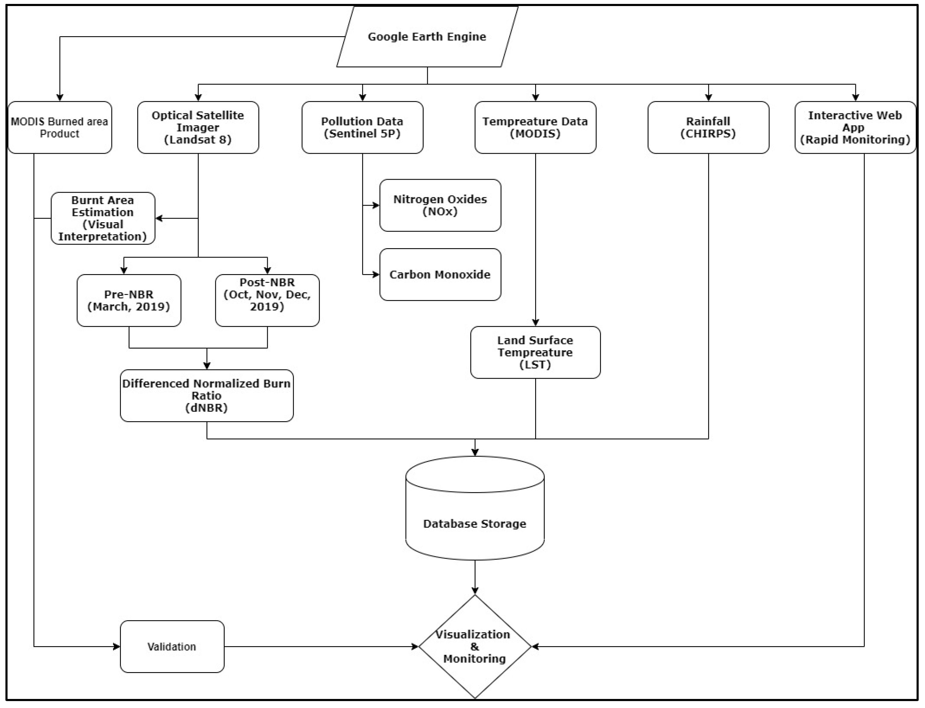
2. Materials and Methods
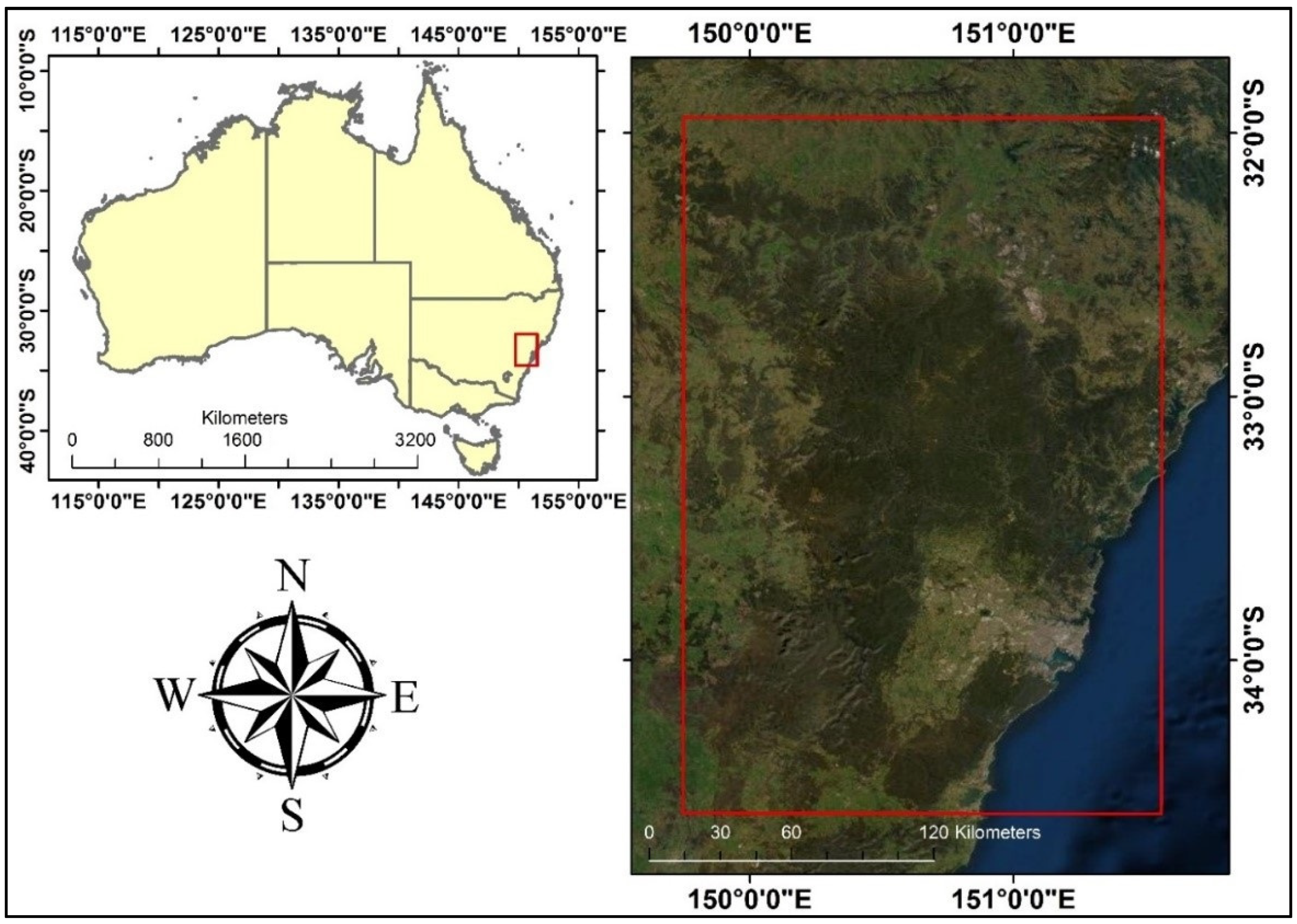
2.1. Study Area
2.2. Materials and Methods
2.2.1. Spectral Indices
2.2.2. Rainfall and Temperature Retrieval
2.2.3. Pollution Monitoring
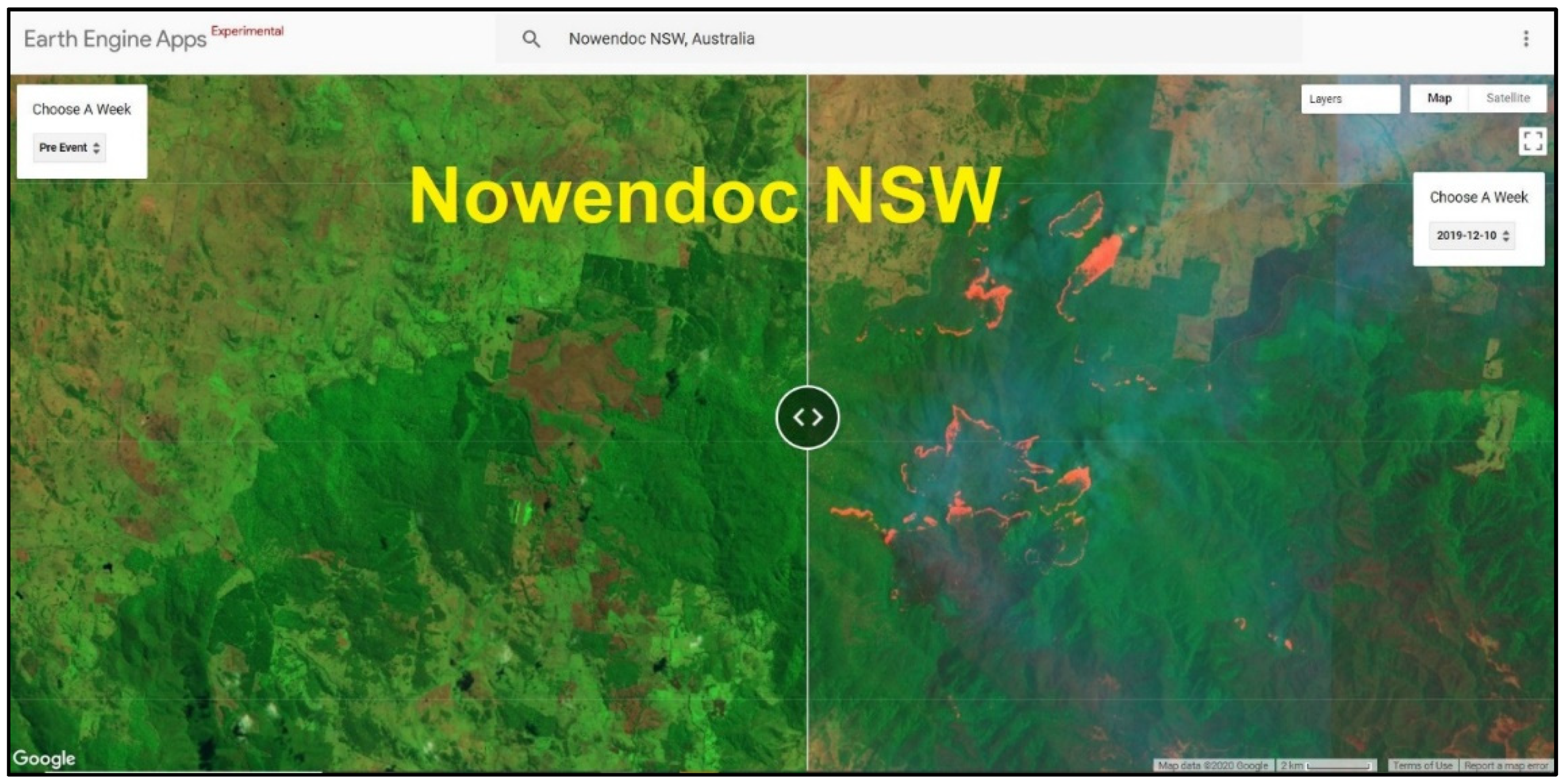
2.2.4. Web-App Development
3. Results and Discussion
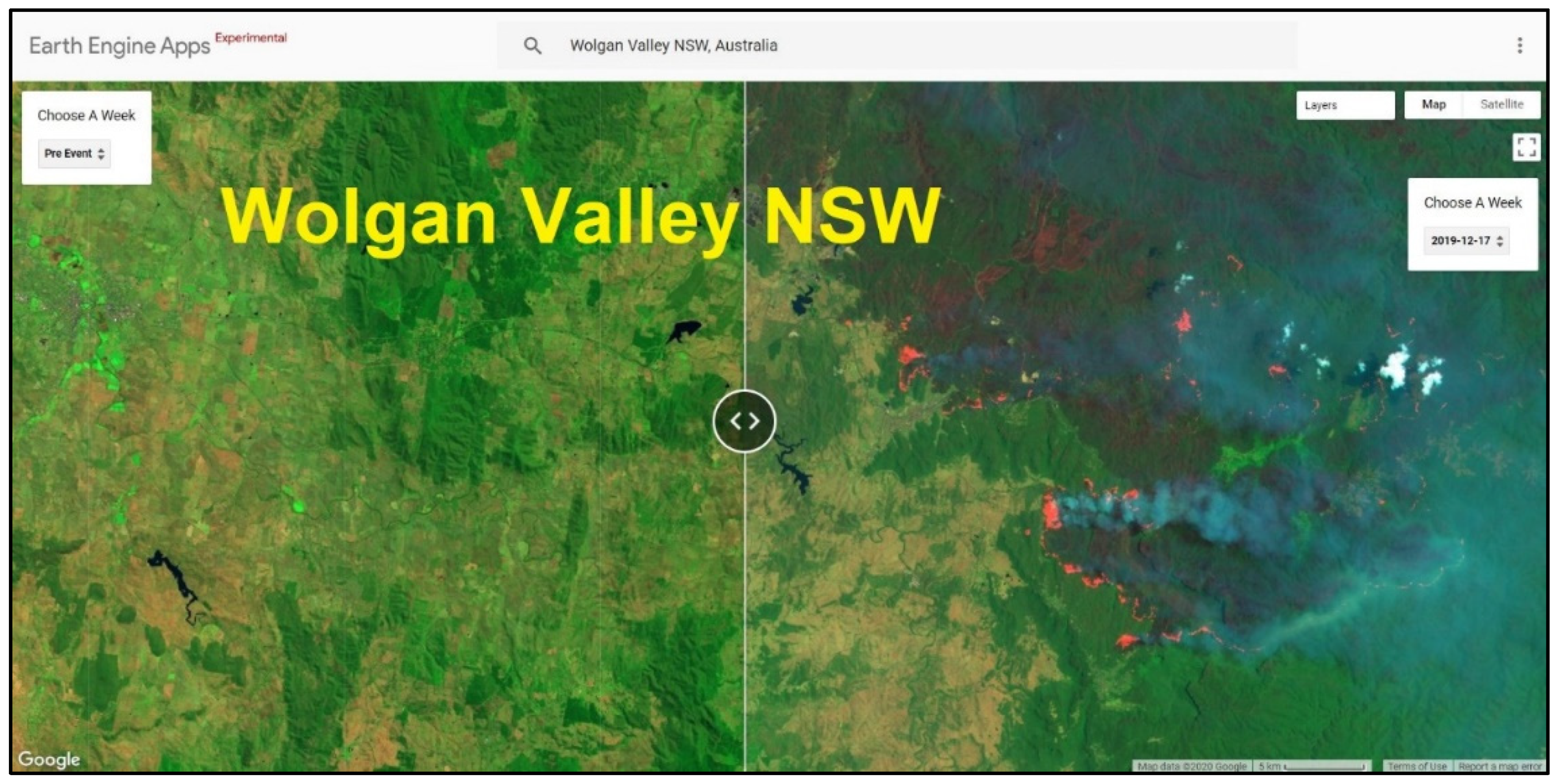
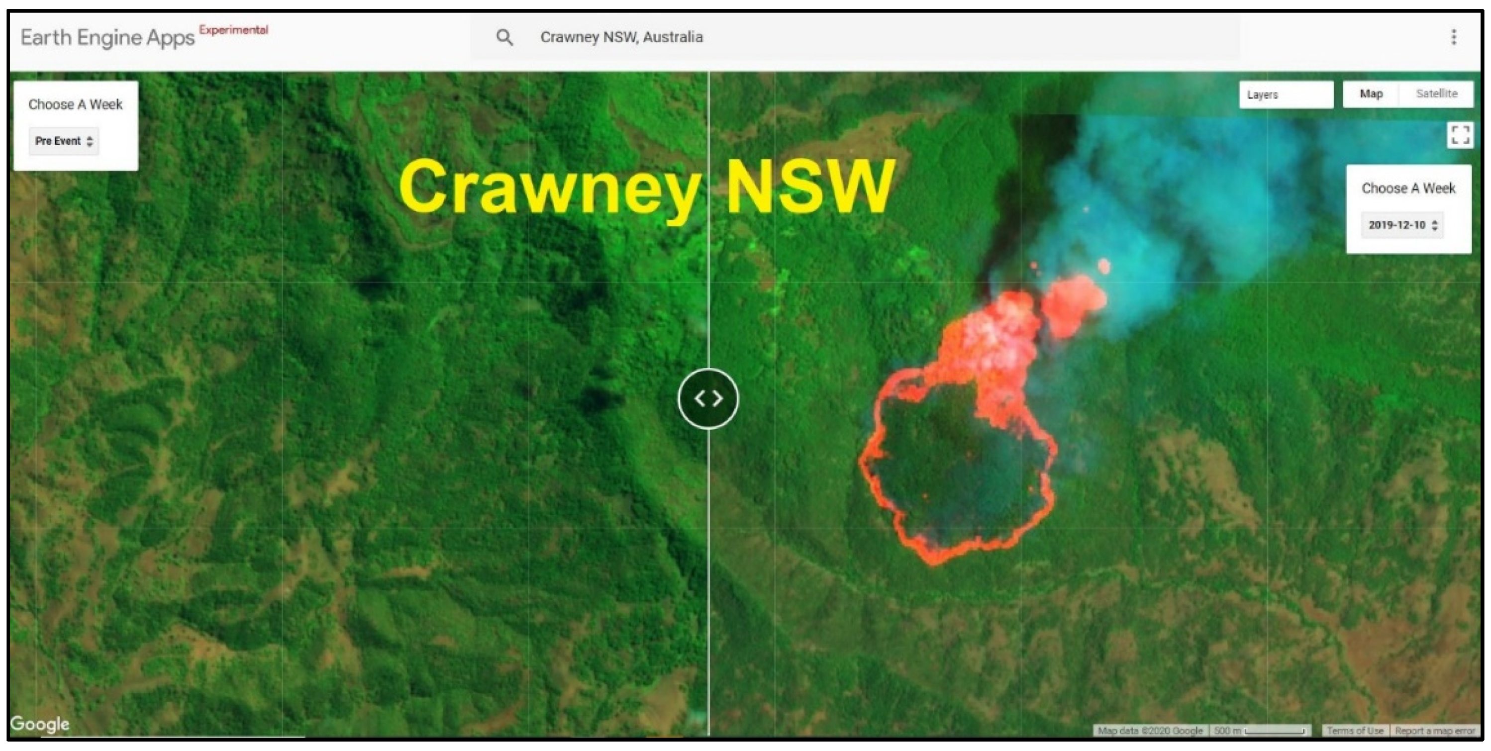
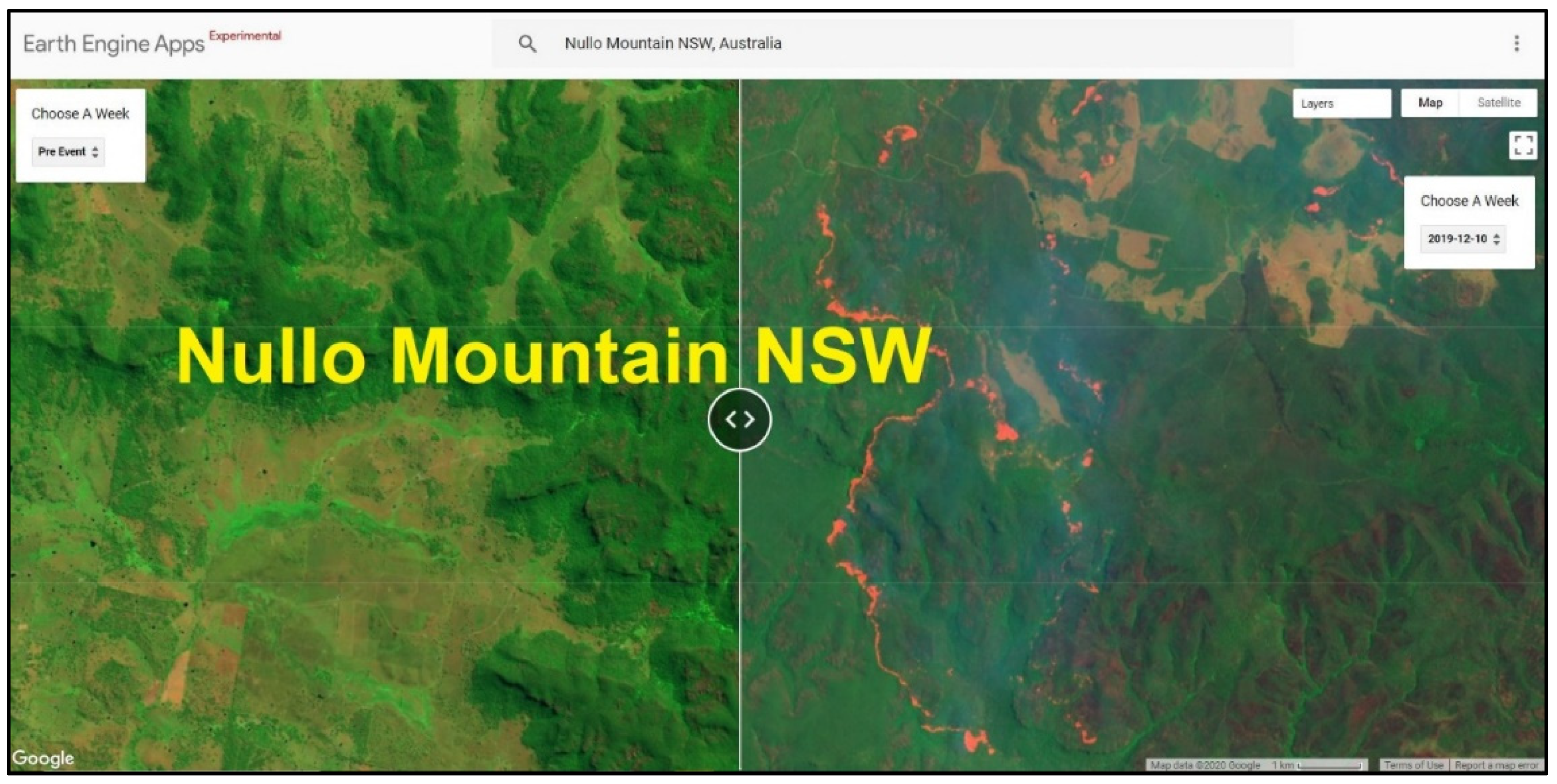
3.1. Web App Visualization
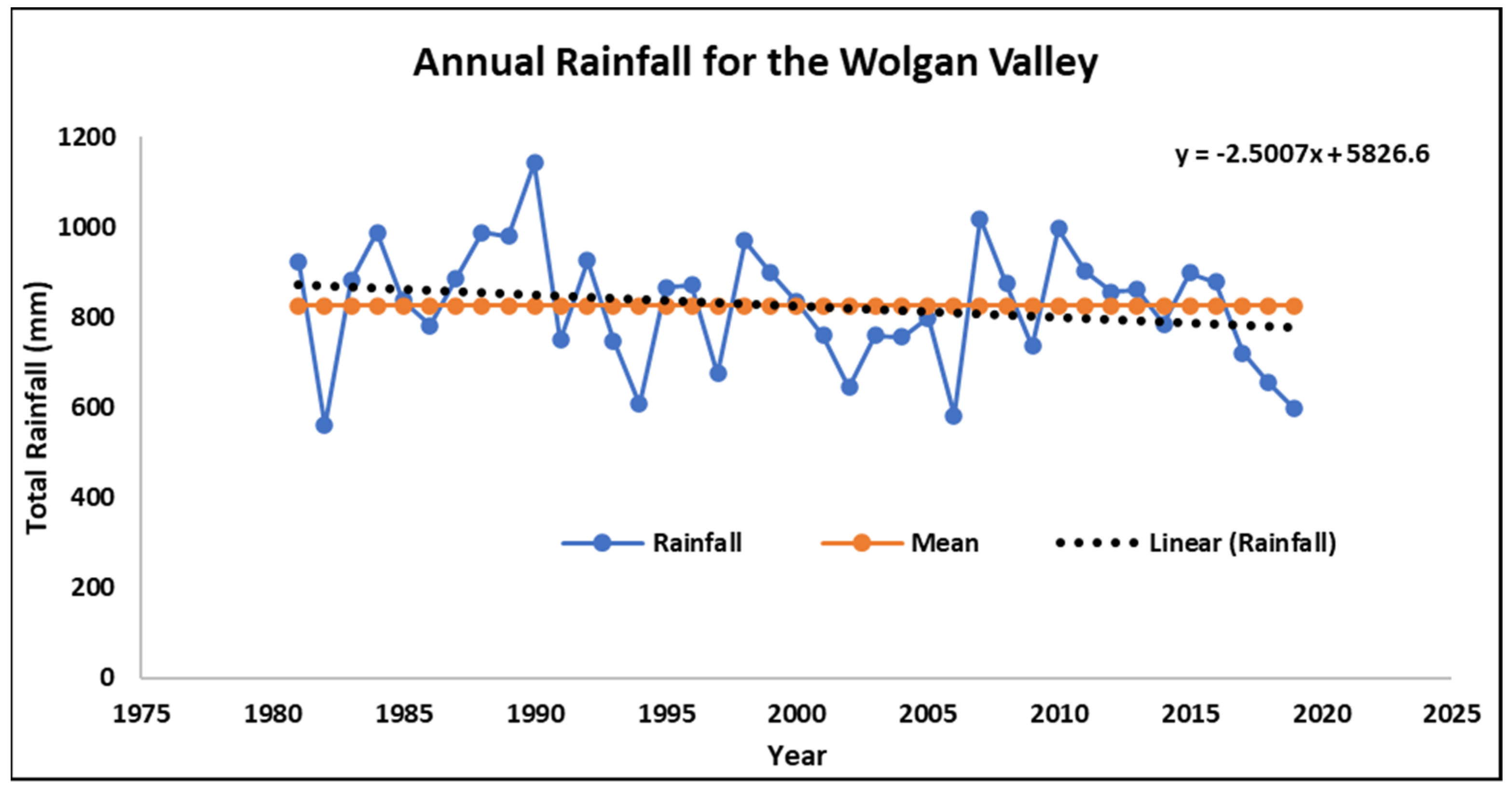
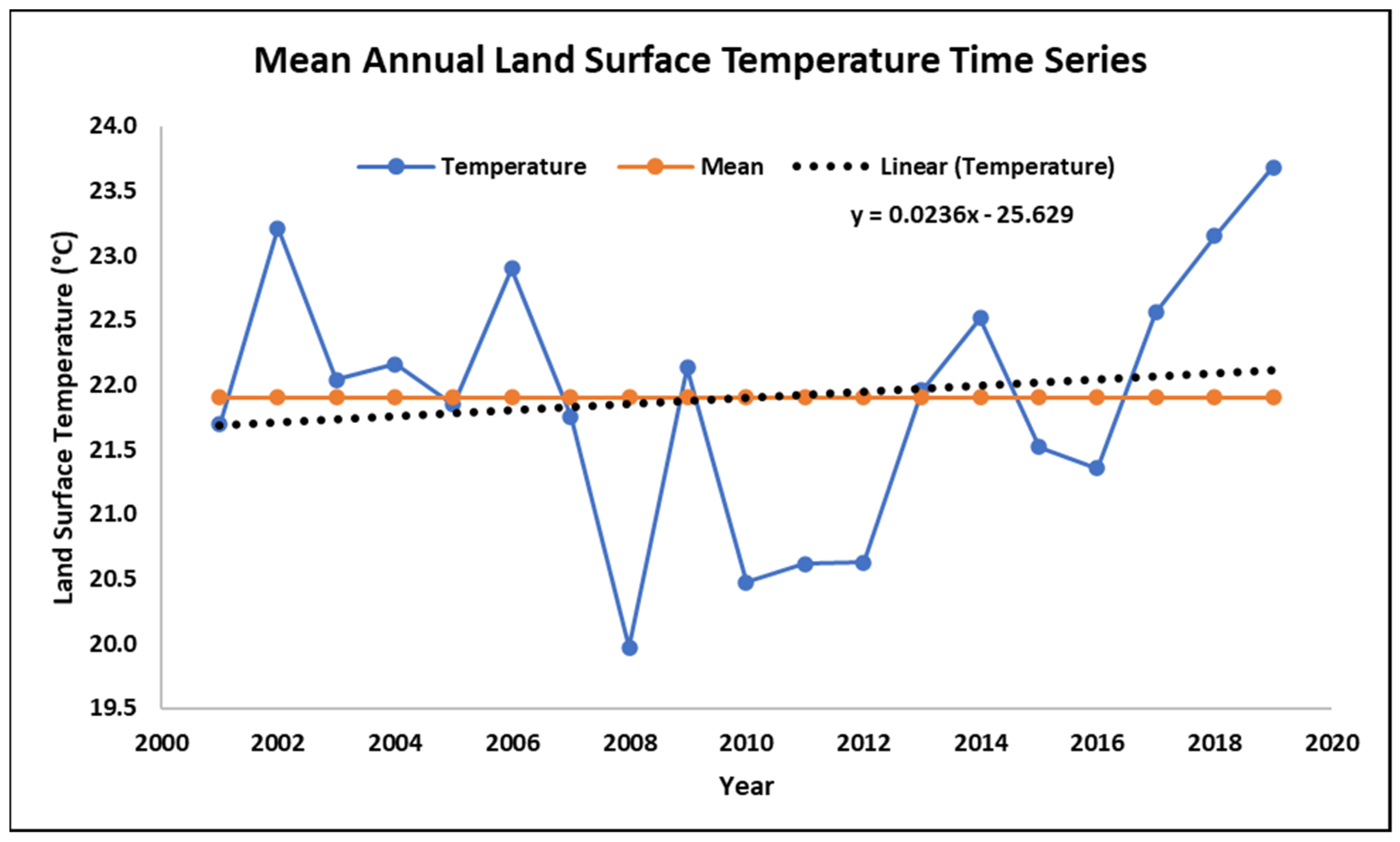
3.2. Rainfall and Temperature Variation
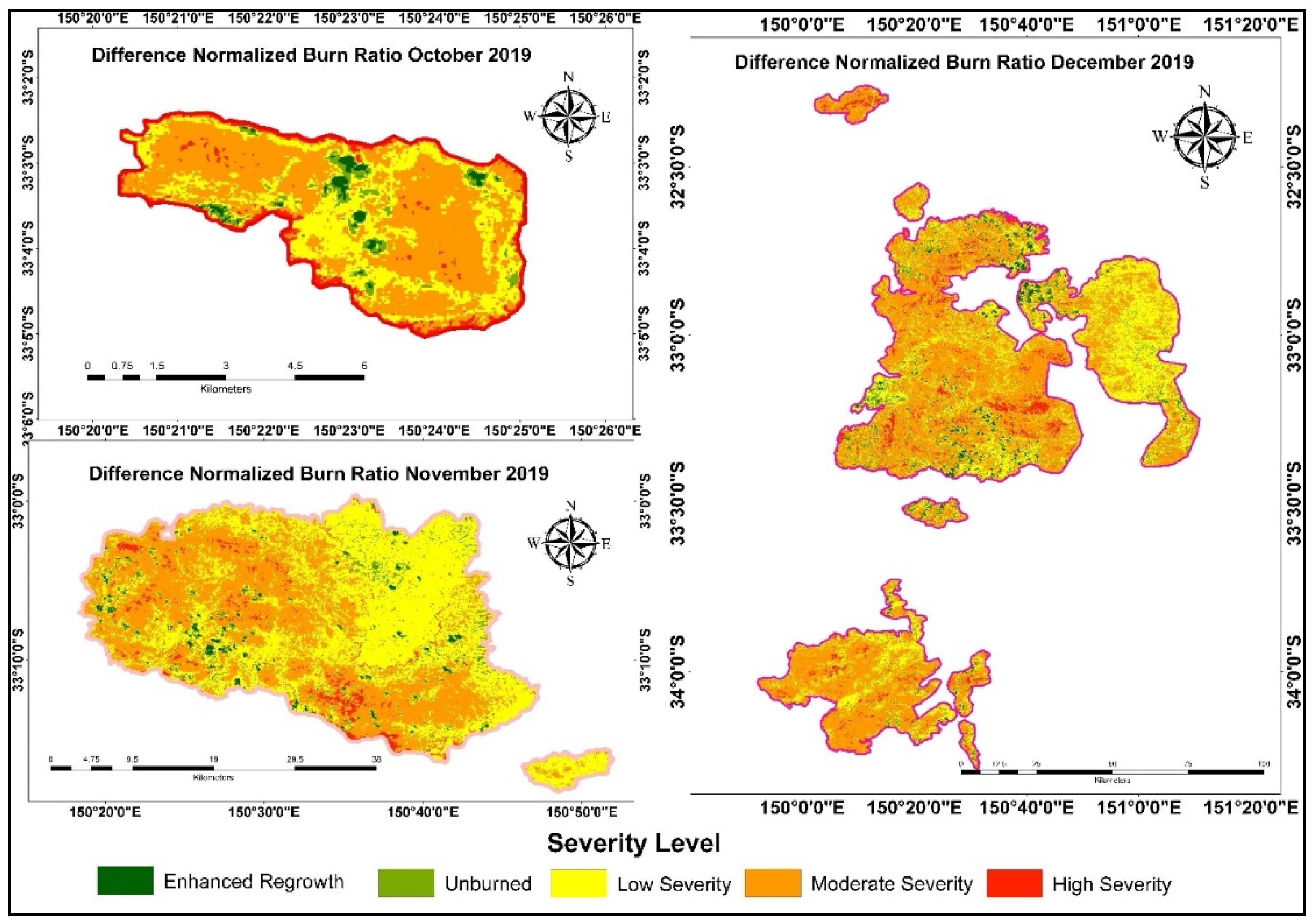
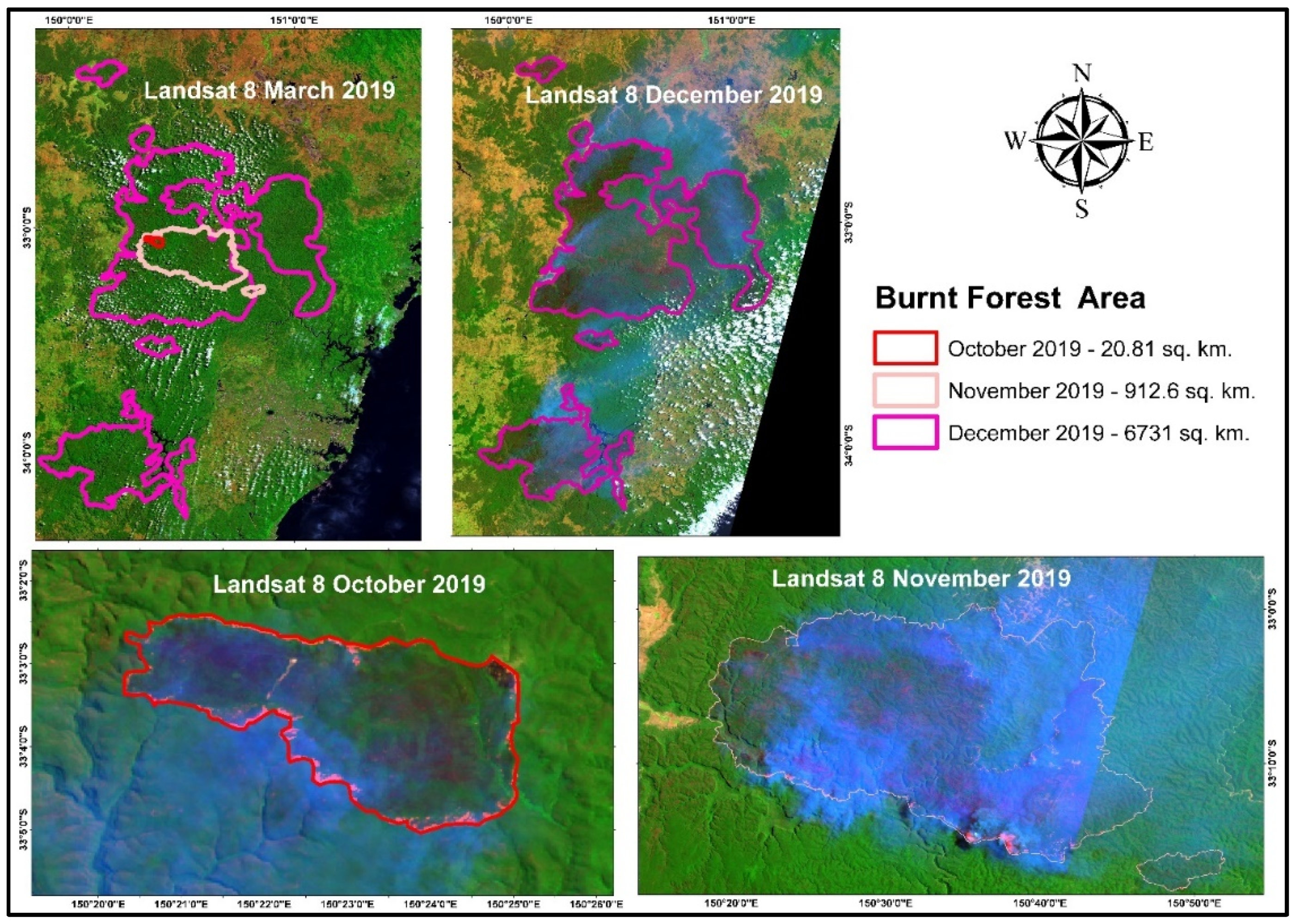
3.3. Burnt Area Estimation
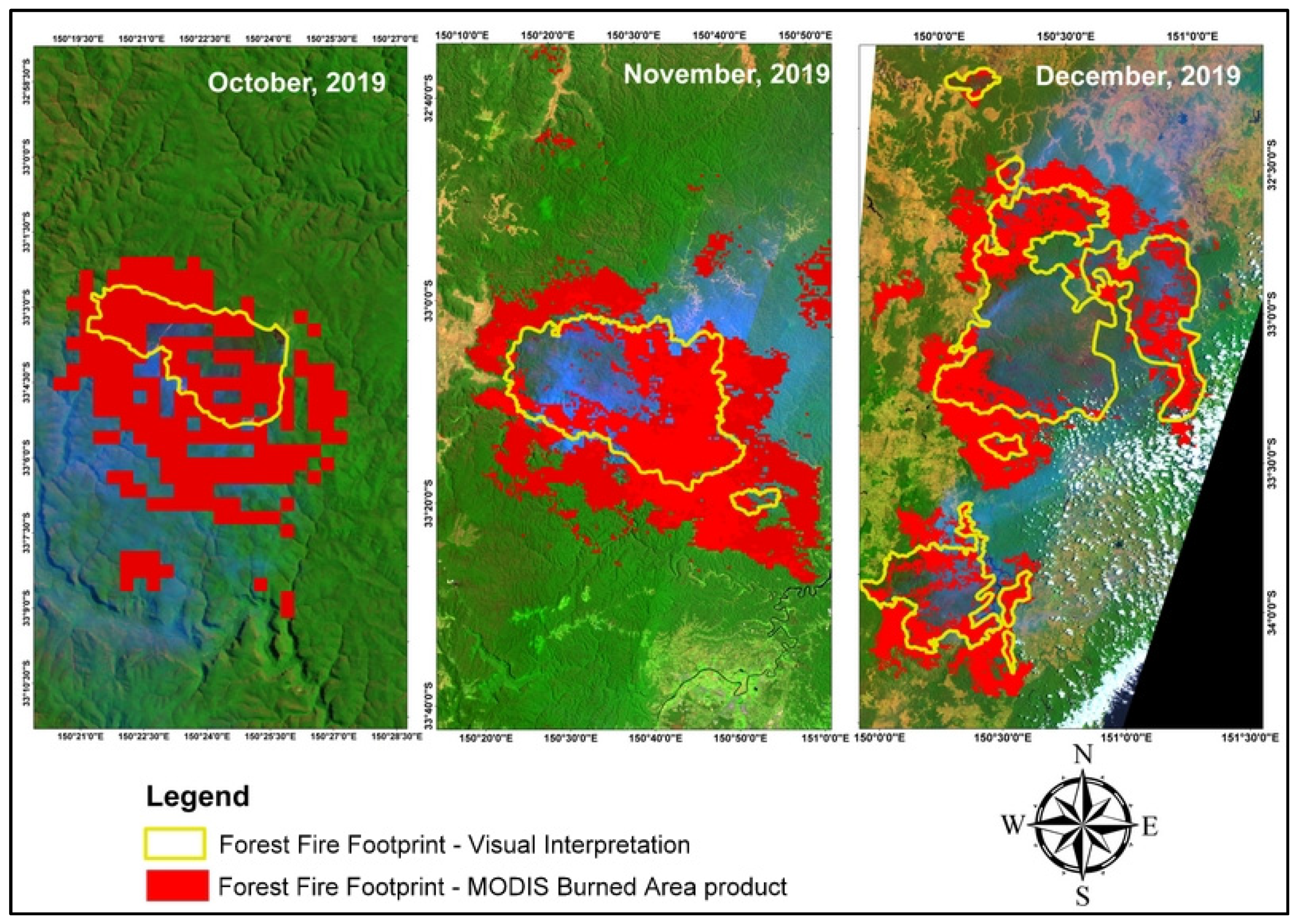
3.4. Validation
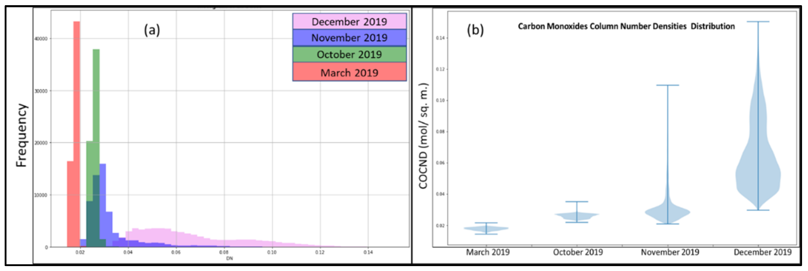
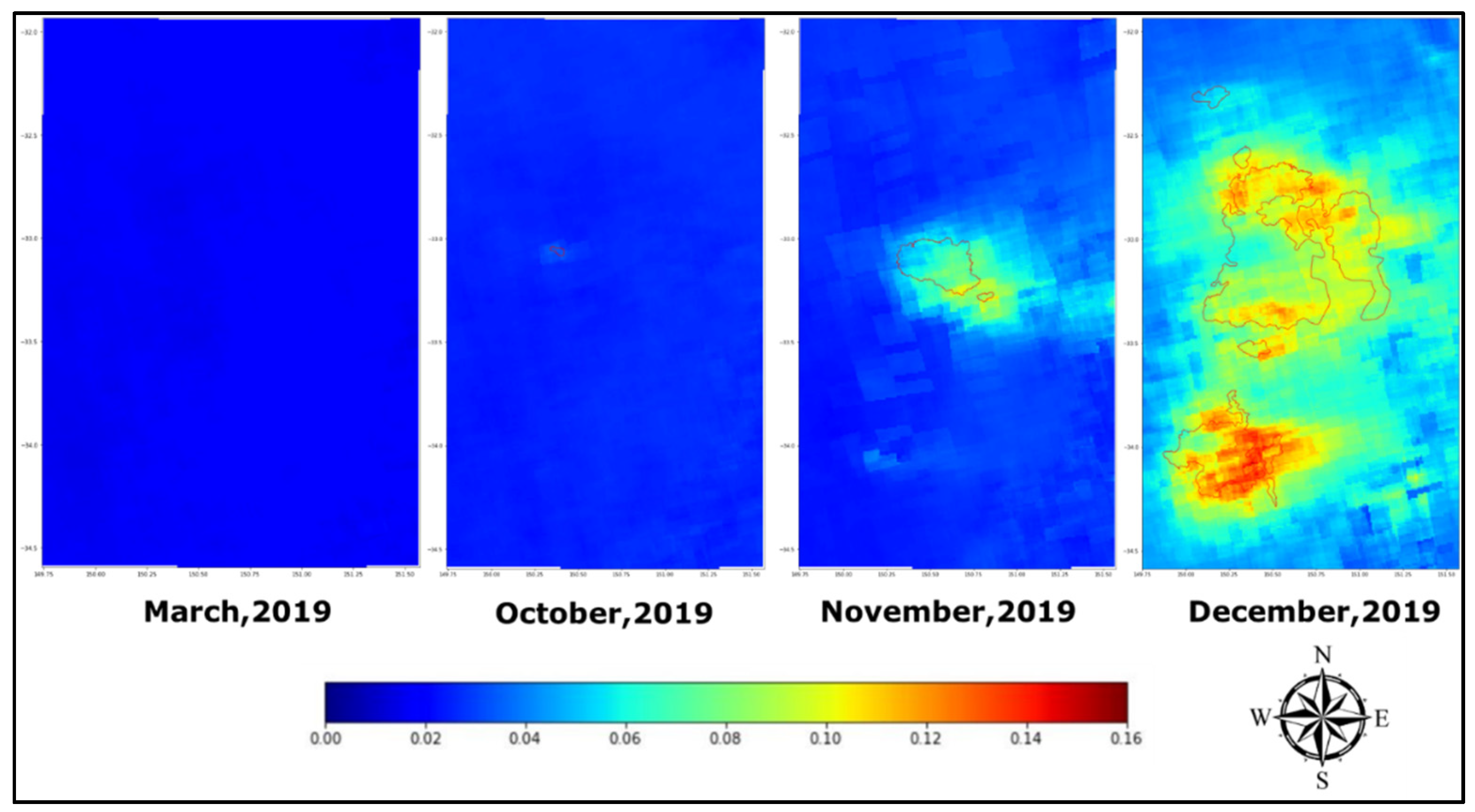
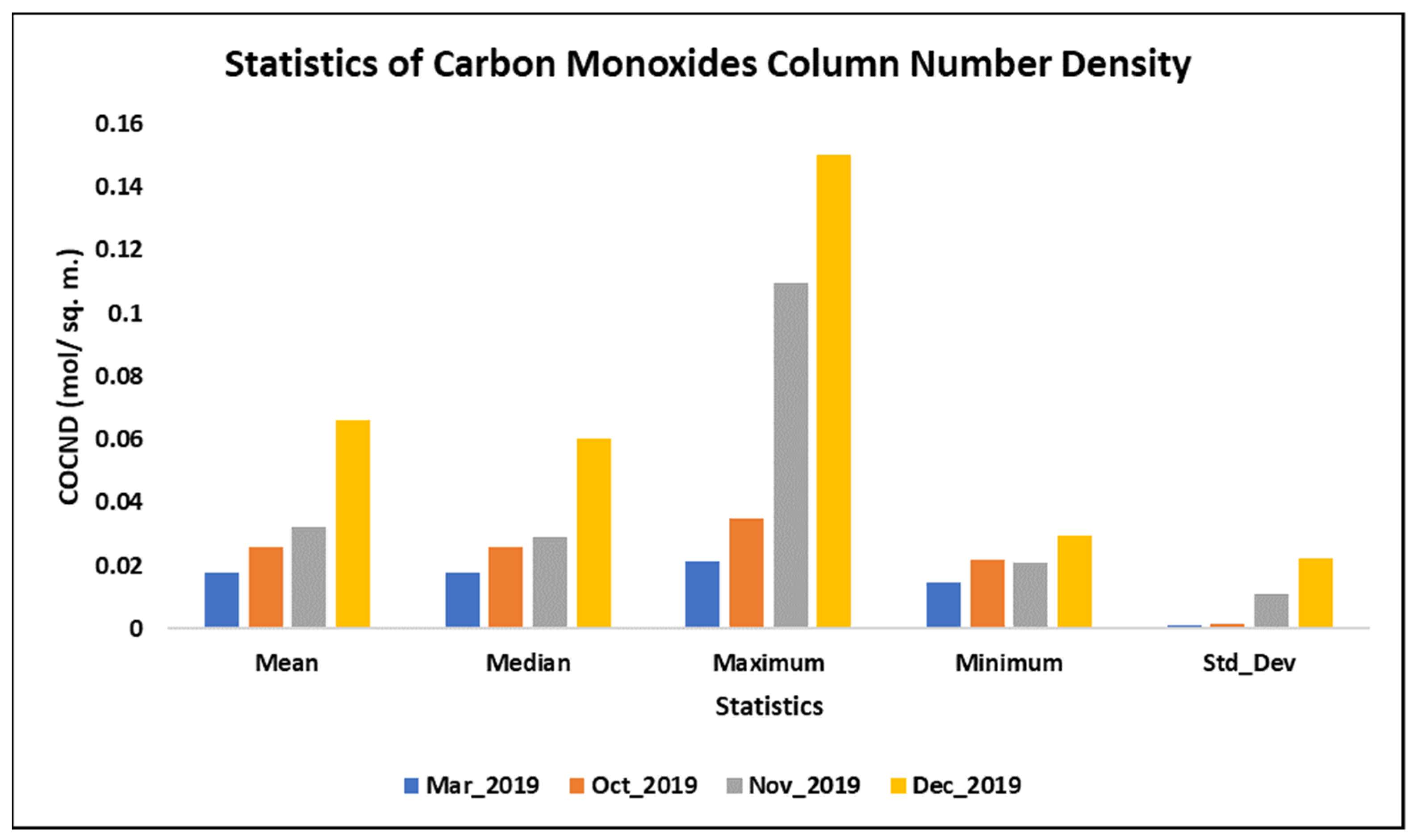
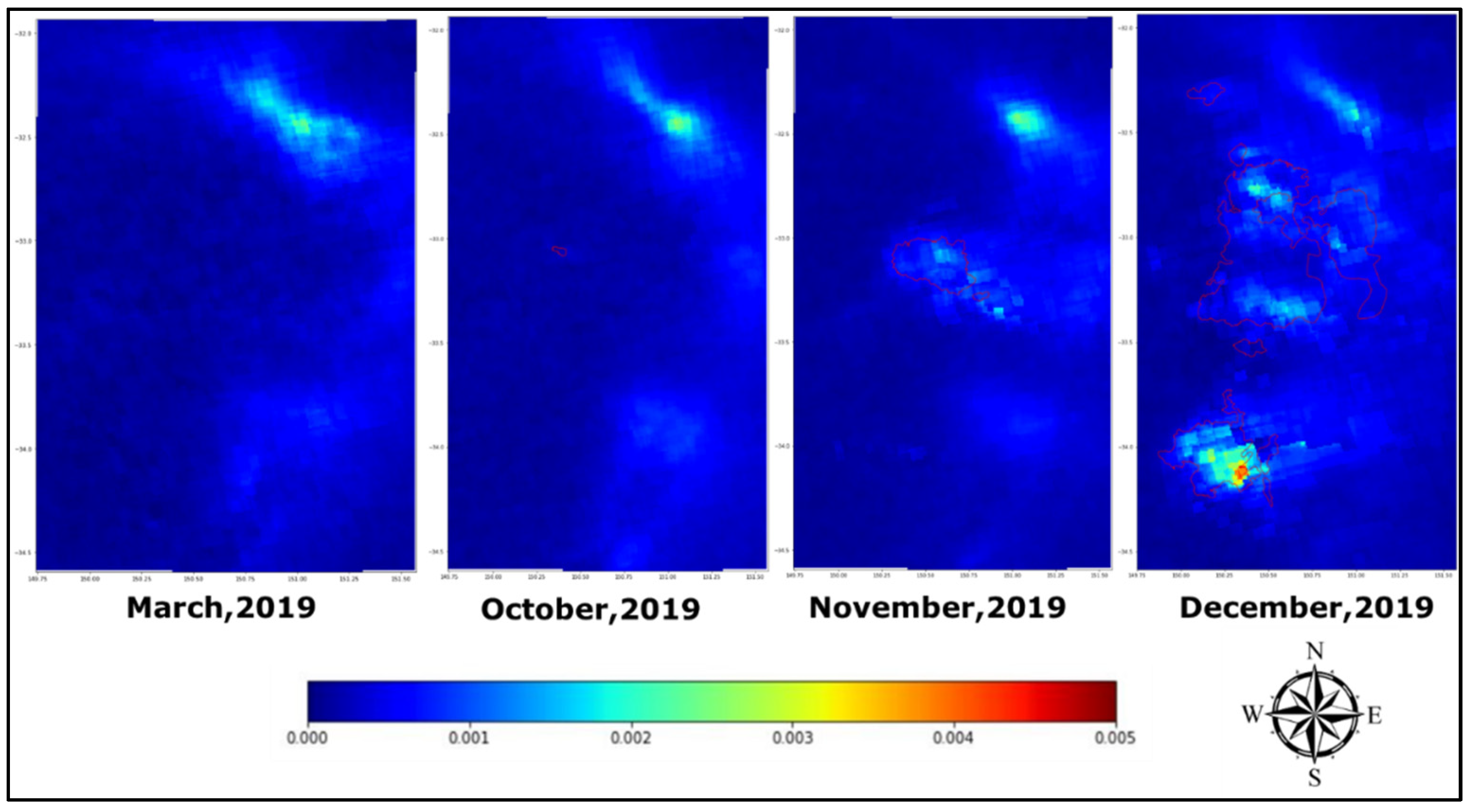
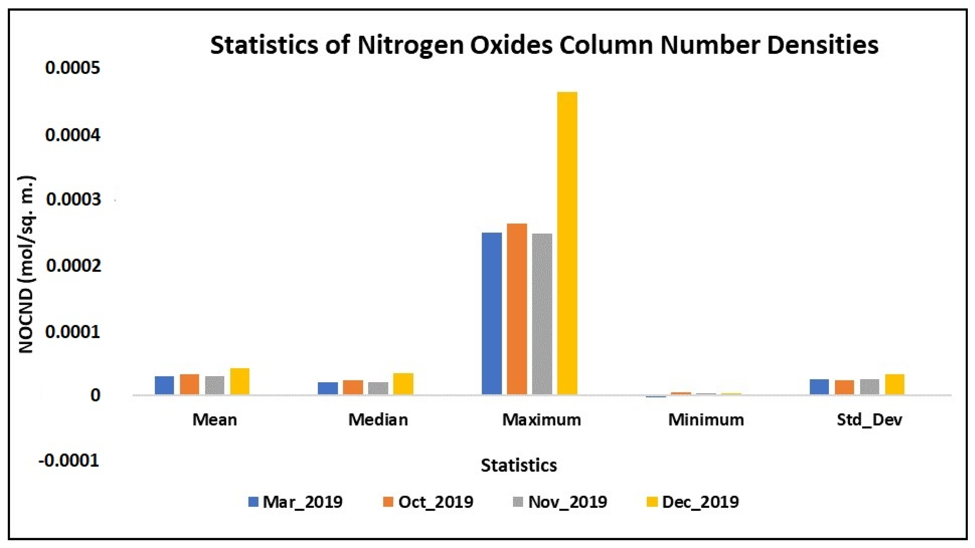
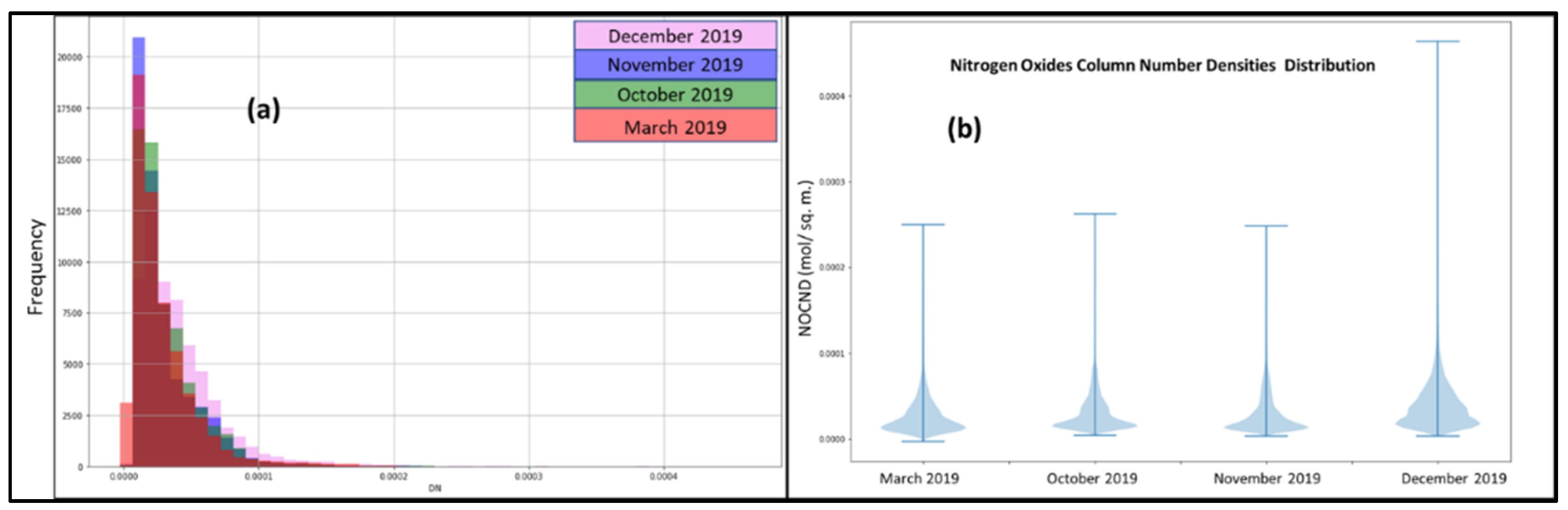
3.5. Impact on Air Pollution Due to the Forest Fire
4. Conclusions
Author Contributions
Funding
Institutional Review Board Statement
Informed Consent Statement
Data Availability Statement
Acknowledgments
Conflicts of Interest
References
- Prasad, A.S.; Pandey, B.W.; Leimgruber, W.; Kunwar, R.M. Mountain hazard susceptibility and livelihood security in the upper catchment area of the river Beas, Kullu Valley, Himachal Pradesh, India. Geoenviron. Disasters 2016, 3, 1. [Google Scholar] [CrossRef] [Green Version]
- Yao, J.; Raffuse, S.M.; Brauer, M.; Williamson, G.J.; Bowman, D.M.; Johnston, F.H.; Henderson, S.B. Predicting the minimum height of forest fire smoke within the atmosphere using machine learning and data from the CALIPSO satellite. Remote Sens. Environ. 2018, 206, 98–106. [Google Scholar] [CrossRef]
- Beck, K.; Mariani, M.; Fletcher, M.-S.; Schneider, L.; Aquino-López, M.; Gadd, P.; Heijnis, H.; Saunders, K.; Zawadzki, A. The impacts of intensive mining on terrestrial and aquatic ecosystems: A case of sediment pollution and calcium decline in cool temperate Tasmania, Australia. Environ. Pollut. 2020, 265, 114695. [Google Scholar] [CrossRef]
- Gibson, R.; Danaher, T.; Hehir, W.; Collins, L. A remote sensing approach to mapping fire severity in south-eastern Australia using sentinel 2 and random forest. Remote Sens. Environ. 2020, 240, 111702. [Google Scholar] [CrossRef]
- Gorelick, N.; Hancher, M.; Dixon, M.; Ilyushchenko, S.; Thau, D.; Moore, R. Google Earth Engine: Planetary-scale geospatial analysis for everyone. Remote Sens. Environ. 2017, 202, 18–27. [Google Scholar] [CrossRef]
- Mab, P.; Ly, S.; Chompuchan, C.; Kositsakulchai, E. Evaluation of Satellite Precipitation from Google Earth Engine in Tonle Sap Basin, Cambodia. In Proceedings of the THA 2019 International Conference on Water Management and Climate Change towards Asia’s Water-Energy-Food Nexus and SDGs, Bangkok, Thailand, 23–25 January 2019. [Google Scholar]
- Singh, S.; Dhasmana, M.K.; Shrivastava, V.; Sharma, V.; Pokhriyal, N.; Thakur, P.K.; Aggarwal, S.P.; Nikam, B.; Garg, V.; Chouksey, A.; et al. Estimation of revised capacity in Gobind Sagar reservoir using Google Earth Engine and GIS. ISPRS—Int. Arch. Photogramm. Remote Sens. Spat. Inf. Sci. 2018, XLII-5, 589–595. [Google Scholar] [CrossRef] [Green Version]
- Chafer, C.J.; Noonan, M.; Macnaught, E. The post-fire measurement of fire severity and intensity in the Christmas 2001 Sydney wildfires. Int. J. Wildland Fire 2004, 13, 227–240. [Google Scholar] [CrossRef]
- Lentile, L.B.; Holden, Z.A.; Smith, A.; Falkowski, M.J.; Hudak, A.T.; Morgan, P.; Lewis, S.A.; Gessler, P.E.; Benson, N.C. Remote sensing techniques to assess active fire characteristics and post-fire effects. Int. J. Wildland Fire 2006, 15, 319–345. [Google Scholar] [CrossRef]
- Miller, J.D.; Thode, A.E. Quantifying burn severity in a heterogeneous landscape with a relative version of the delta Normalized Burn Ratio (dNBR). Remote Sens. Environ. 2007, 109, 66–80. [Google Scholar] [CrossRef]
- Kasischke, E.S.; Turetsky, M.R.; Ottmar, R.D.; French, N.H.F.; Hoy, E.E.; Kane, E.S. Evaluation of the composite burn index for assessing fire severity in Alaskan black spruce forests. Int. J. Wildland Fire 2008, 17, 515–526. [Google Scholar] [CrossRef]
- Smith, A.M.; Eitel, J.U.; Hudak, A.T. Spectral analysis of charcoal on soils: Implications for wildland fire severity mapping methods. Int. J. Wildland Fire 2010, 19, 976–983. [Google Scholar] [CrossRef]
- Marino, E.; Guillen-Climent, M.; Ranz Vega, P.; Tomé, J. Fire severity mapping in Garajonay National Park: Comparison between spectral indices. FLAMMA 2016, 7, 22–28. [Google Scholar]
- Soverel, N.O.; Perrakis, D.D.; Coops, N.C. Estimating burn severity from Landsat dNBR and RdNBR indices across western Canada. Remote Sens. Environ. 2010, 114, 1896–1909. [Google Scholar] [CrossRef]
- Meng, Q.; Meentemeyer, R.K. Modeling of multi-strata forest fire severity using Landsat TM Data. Int. J. Appl. Earth Obs. Geoinf. 2011, 13, 120–126. [Google Scholar] [CrossRef]
- Escuin, S.; Navarro, R.; Fernández, P. Fire severity assessment by using NBR (Normalized Burn Ratio) and NDVI (Normalized Difference Vegetation Index) derived from LANDSAT TM/ETM images. Int. J. Remote Sens. 2007, 29, 1053–1073. [Google Scholar] [CrossRef]
- Kollanus, V.; Tiittanen, P.; Niemi, J.; Lanki, T. Effects of long-range transported air pollution from vegetation fires on daily mortality and hospital admissions in the Helsinki metropolitan area, Finland. Environ. Res. 2016, 151, 351–358. [Google Scholar] [CrossRef]
- McMahon, C.K. Forest fires and smoke—Impacts on air quality and human health in the USA. In Proceedings of the TAPPI International Environmental Conference, Nashville, TN, USA, 18–21 April 1999; TAPPI Press: Nashville, TN, USA, 1999; Volume 2, pp. 443–453. [Google Scholar]
- Yin, S.; Wang, X.; Guo, M.; Santoso, H.; Guan, H. The abnormal change of air quality and air pollutants induced by the forest fire in Sumatra and Borneo in 2015. Atmos. Res. 2020, 243, 105027. [Google Scholar] [CrossRef]
- Yuchi, W.; Yao, J.; McLean, K.E.; Stull, R.; Pavlovic, R.; Davignon, D.; Moran, M.D.; Henderson, S.B. Blending forest fire smoke forecasts with observed data can improve their utility for public health applications. Atmos. Environ. 2016, 145, 308–317. [Google Scholar] [CrossRef]
- Adetona, O.; Reinhardt, T.E.; Domitrovich, J.; Broyles, G.; Adetona, A.; Kleinman, M.T.; Ottmar, R.D.; Naeher, L.P. Review of the health effects of wildland fire smoke on wildland firefighters and the public. Inhal. Toxicol. 2016, 28, 95–139. [Google Scholar] [CrossRef]
- Langmann, B.; Duncan, B.; Textor, C.; Trentmann, J.; van der Werf, G. Vegetation fire emissions and their impact on air pollution and climate. Atmos. Environ. 2009, 43, 107–116. [Google Scholar] [CrossRef]
- Bernard, M.; Bernard, L. Correlation between Wildfire Statistical Data, Weather and Climate. 2007. Available online: https://ams.confex.com/ams/pdfpapers/126829.pdf (accessed on 20 August 2021).
- Trauernicht, C. Vegetation—Rainfall interactions reveal how climate variability and climate change alter spatial patterns of wildland fire probability on Big Island, Hawaii. Sci. Total Environ. 2019, 650, 459–469. [Google Scholar] [CrossRef] [PubMed]
- Whitworth-Hulse, J.I.; Magliano, P.N.; Zeballos, S.R.; Gurvich, D.E.; Spalazzi, F.; Kowaljow, E. Advantages of rainfall partitioning by the global invader Ligustrum lucidum over the dominant native Lithraea molleoides in a dry forest. Agric. For. Meteorol. 2020, 290, 108013. [Google Scholar] [CrossRef]
- Bar, S.; Parida, B.R.; Pandey, A.C. Landsat-8 and Sentinel-2 based Forest fire burn area mapping using machine learning algorithms on GEE cloud platform over Uttarakhand, Western Himalaya. Remote Sens. Appl. Soc. Environ. 2020, 18, 100324. [Google Scholar] [CrossRef]
- Burton, J. It Was a Line of Fire Coming at Us’: South West Firefighters Return Home. 2020. Available online: https://www.busseltonmail.com.au/story/6620313/it-was-a-line-of-fire-coming-at-us-firefighters-return-home/ (accessed on 20 August 2021).
- ABCNews. Victorian Bushfires Death Toll Rises as Authorities Confirm Contractor’s Death Was Fire-Related. 2020. Available online: https://www.abc.net.au/news/2020-01-15/fires-death-toll-rises-to-five-in-victoria/11869596 (accessed on 20 August 2021).
- Green, M. Australia’s Massive Fires Could Become Routine, Climate Scientists Warn. 2020. Available online: https://www.reuters.com/article/us-climate-change-australia-report/australias-massive-fires-could-become-routine-climate-scientists-warn-idUSKBN1ZD06W (accessed on 20 August 2021).
- SBSNews. The Numbers Behind Australia’s Catastrophic Bushfire Season. 2020. Available online: https://www.sbs.com.au/news/the-numbers-behind-australia-s-catastrophic-bushfire-season (accessed on 20 August 2021).
- O’Mallon, F.; Tiernan, E. Australia’s 2019–2020 Bushfire Season. 2020. Available online: https://www.canberratimes.com.au/story/6574563/australias-2019-20-bushfire-season/ (accessed on 20 August 2021).
- Readfearn, G. “Silent Death”: Australia’s Bushfires Push Countless Species to Extinction. 2020. Available online: https://www.theguardian.com/environment/2020/jan/04/ecologists-warn-silent-death-australia-bushfires-endangered-species-extinction (accessed on 20 August 2021).
- The University of Sydney. More Than One Billion Animals Killed in Australian Bushfires. 2020. Available online: https://www.sydney.edu.au/news-opinion/news/2020/01/08/australian-bushfires-more-than-one-billion-animals-impacted.html (accessed on 20 August 2021).
- Zaman, M.A.; Rahman, A.; Haddad, K. Regional flood frequency analysis in arid regions: A case study for Australia. J. Hydrol. 2012, 475, 74–83. [Google Scholar] [CrossRef]
- Veraverbeke, S.; Lhermitte, S.; Verstraeten, W.; Goossens, R. The temporal dimension of differenced Normalized Burn Ratio (dNBR) fire/burn severity studies: The case of the large 2007 Peloponnese wildfires in Greece. Remote Sens. Environ. 2010, 114, 2548–2563. [Google Scholar] [CrossRef] [Green Version]
- Roy, D.P.; Boschetti, L.; Trigg, S.N. Remote sensing of fire severity: Assessing the performance of the normalized burn ratio. IEEE Geosci. Remote Sens. Lett. 2006, 3, 112–116. [Google Scholar] [CrossRef] [Green Version]
- Teobaldo, D.; Baptista, G.M.D.E. Measurement of severity of fires and loss of carbon forest sink in the conservation units at Distrito Federal. Rev. Bras. Geogr. Fis. 2016, 9, 250–264. [Google Scholar] [CrossRef] [Green Version]
- Key, C.H.; Benson, N.C. Landscape Assessment: Ground Measure of Severity, the Composite Burn Index; and Remote Sensing of Severity, the Normalized Burn Ratio. 2006. Available online: http://pubs.er.usgs.gov/publication/2002085 (accessed on 20 August 2021).
- Dos Santos, S.M.B.; Bento-Gonçalves, A.; Franca-Rocha, W.; Baptista, G. Assessment of burned forest area severity and postfire regrowth in chapada diamantina national park (Bahia, Brazil) using dnbr and rdnbr spectral indices. Geosciences 2020, 10, 106. [Google Scholar] [CrossRef] [Green Version]


| S. No. | Purpose | Data | Duration | Resolution/Scale | Source |
|---|---|---|---|---|---|
| 1 | Burned Area Mapping | LANDSAT-8 Operational Land Imager | March, October, November, December 2019 | 30 m | Google Earth Engine https://code.earthengine.google.com/ (Accessed on 20 August 2021). |
| 2 | Web App Visualization | Sentinel 2 | March, October, November, December 2019 | 10 m | |
| 3 | Rainfall | CHIRPS daily | 1981–2019 | 5000 m | |
| 4 | Land Surface Temperature | MODIS Terra LST daily | 2001–2019 | 1000 m | |
| 5 | Pollution Mapping and Monitoring | Sentinel 5P | March, October, November, December 2019 | 1000 m | |
| 6 | Validation | MODIS Burned Area Monthly | October, November, December 2019 | 500 m |
| Time Period | Trend | h | p | z | Tau | s | var_s | Slope | Intercept |
|---|---|---|---|---|---|---|---|---|---|
| Yearly | no trend | FALSE | 0.110313 | −1.59679 | −0.17949 | −133 | 6833.667 | −0.55886 | 48.80874 |
| 2-yearly moving average | no trend | FALSE | 0.056014 | −1.91093 | −0.21764 | −153 | 6327 | −0.48733 | 48.69761 |
| 3-yearly moving average | decreasing | TRUE | 0.008567 | −2.62886 | −0.3033 | −202 | 5846 | −0.56612 | 53.42137 |
| 4-yearly moving average | decreasing | TRUE | 0.001132 | −3.25539 | −0.38095 | −240 | 5390 | −0.66736 | 58.51139 |
| 5-yearly moving average | decreasing | TRUE | 0.000222 | −3.69237 | −0.43866 | −261 | 4958.333 | −0.72488 | 61.15642 |
| Month | Theoretical Range | NBR |
|---|---|---|
| Mar-19 | [−1 to 1] | [−0.68 to +1] |
| Oct-19 | [−1 to 1] | [−0.77 to +1] |
| Nov-19 | [−1 to 1] | [−0.86 to +1] |
| Dec-19 | [−1 to 1] | [−0.87 to +0.88] |
| Severity Level | dNBR Range |
|---|---|
| Enhanced Regrowth | [>−0.1] |
| Unburned | [−0.1 to +0.1] |
| Low Severity | [+0.1 to +0.27] |
| Moderate Severity | [+0.27 to +0.66] |
| High Severity | [>+0.66] |
Publisher’s Note: MDPI stays neutral with regard to jurisdictional claims in published maps and institutional affiliations. |
© 2021 by the authors. Licensee MDPI, Basel, Switzerland. This article is an open access article distributed under the terms and conditions of the Creative Commons Attribution (CC BY) license (https://creativecommons.org/licenses/by/4.0/).
Share and Cite
Singh, S.; Singh, H.; Sharma, V.; Shrivastava, V.; Kumar, P.; Kanga, S.; Sahu, N.; Meraj, G.; Farooq, M.; Singh, S.K. Impact of Forest Fires on Air Quality in Wolgan Valley, New South Wales, Australia—A Mapping and Monitoring Study Using Google Earth Engine. Forests 2022, 13, 4. https://doi.org/10.3390/f13010004
Singh S, Singh H, Sharma V, Shrivastava V, Kumar P, Kanga S, Sahu N, Meraj G, Farooq M, Singh SK. Impact of Forest Fires on Air Quality in Wolgan Valley, New South Wales, Australia—A Mapping and Monitoring Study Using Google Earth Engine. Forests. 2022; 13(1):4. https://doi.org/10.3390/f13010004
Chicago/Turabian StyleSingh, Sachchidanand, Harikesh Singh, Vishal Sharma, Vaibhav Shrivastava, Pankaj Kumar, Shruti Kanga, Netrananda Sahu, Gowhar Meraj, Majid Farooq, and Suraj Kumar Singh. 2022. "Impact of Forest Fires on Air Quality in Wolgan Valley, New South Wales, Australia—A Mapping and Monitoring Study Using Google Earth Engine" Forests 13, no. 1: 4. https://doi.org/10.3390/f13010004
APA StyleSingh, S., Singh, H., Sharma, V., Shrivastava, V., Kumar, P., Kanga, S., Sahu, N., Meraj, G., Farooq, M., & Singh, S. K. (2022). Impact of Forest Fires on Air Quality in Wolgan Valley, New South Wales, Australia—A Mapping and Monitoring Study Using Google Earth Engine. Forests, 13(1), 4. https://doi.org/10.3390/f13010004