Investments in Pinus elliottii Engelm. Plantations: Real Options Analysis in Discrete Time

Abstract

Background: The commonly used methods for the financial evaluation of plantation forest investment projects do not incorporate uncertainties and ignore the value related to flexibility. The real options analysis makes it possible to capture these values in investment projects, increasing their value and return. Despite this, studies involving real options in forest investment projects are scarce, specifically those related to Pinus spp. Therefore, this study aimed to: (a) analyze whether the real options analysis adds value to investment projects of Pinus elliottii Engelm. plantations; and (b) make the real options analysis more accessible to forest managers and potentially increase its use in the investment projects of Pinus spp. plantations. Methods: We evaluated two investment projects in P. elliottii plantations in southern Brazil, which differed in the way of obtaining the land for planting: with lease or purchase of land on a planning horizon of 21 years. In the real options analysis, we used deferral, expansion, and abandonment. Results: Individually, the deferral, expansion, and abandonment options add value to investment projects in Pinus elliottii plantations. The option to expand the forested area is one that adds the most value to the investment project with land lease. In the investment project with land purchase, it is abandonment. Conclusions: Investment projects in Pinus elliotti plantations that contemplate the land purchase analyzed through the real options analysis present higher financial returns than those that consider land lease, inverting the result provided by the traditional analysis.

1. Introduction

The forest plantations require important financial contributions because they are being long-term projects, usually under conditions of uncertainty, with managerial flexibilities that can be exercised over the useful life of the biological asset. In addition to the financial aspect, the forest plantations provide multiple ecosystem services like supporting (e.g., nutrient cycling), provisioning (e.g., wood and non-wood forest products, and fresh water production), regulating (e.g., local climate regulation, carbon sequestration and storage, and preventing soil erosion), and cultural (e.g., aesthetic values, recreation, and eco-tourism) when compared to previously deforested lands [1,2,3,4].

The planting of homogeneous forests has been increasing in order to meet the growing demand for wood in world markets [5]. In Brazil, the area of forest plantations totals 9.6 million hectares. Of this total, 19.0% represents Pinus spp., with 1.8 million hectares [6].

Forest management integrates silvicultural practices and business concepts, as economic alternatives, in order to better achieve the investor’s objectives [7]. The analysis of a forest investment involves the use of techniques and criteria that compare costs and revenues inherent to the project, aiming to verify whether or not it should be implemented [8].

The commonly used methods for the financial evaluation of forest investment projects are those based on performance metrics, among which is net present value (NPV). However, NPV does not incorporate uncertainties and ignores the value related to flexibility, that is, management is not able to adapt and review decisions in response to changes in market conditions [9,10,11]. The forest investment projects have a higher cost in the first months of planting and revenues, in general, occur at the end of their useful life. Traditional methods of financial evaluation do not provide the necessary flexibility in the face of inherent uncertainties of the forest sector and can present an obstacle to new business [12].

The price of wood, for example, has associated uncertainties that culminate in price fluctuations mainly due to the volatility of wood demand in the forest sector [13]. Reliable price and wood production estimates, as well as the calculation of criteria that include uncertainty, are necessary to make the decision-making process more robust [14]. The stochastic methods of investment analysis contemplate investors with possibilities that add value to the project, exploring uncertainties and, consequently, managerial flexibilities.

When considering managerial flexibility, managers can better evaluate project alternatives and allocate capital resources more efficiently [15]. The value of flexibility allows the decision-maker to decide what to do after some of the uncertainties related to the future are at least partially resolved [16,17,18].

The real options analysis makes it possible to capture the value of managerial flexibilities in investment projects [19,20,21,22] by means of options available throughout the life of the project, increasing its value and return. This is possible when management uses real options as a way to limit possible losses and enhance or protect positive results [23,24,25] in environments with irreversibility and uncertainties, like the forest sector [26,27,28,29,30].

A real option is a right, not an obligation, to execute a particular investment project or to make certain decisions in more advanced stages of the project [25,31,32,33] at a predetermined cost called the exercise price of the option. The real value of an investment project can be assessed by combining the value provided by real options of this investment with the value of the result of traditional static NPV [34,35]. However, as real options are usually not traded in the market, each one is exclusively defined by its context and needs a personalized assessment [36].

Among the methods used to calculate the value of real options is the discrete-time binomial model (CRR) [37]. The CRR model is also called the binomial tree, as the pricing process is to build a binomial tree to evaluate underlying assets over a given period of time [37,38]. This model is one of the most common tools for real options and its structure provides greater modeling flexibility to analyze multiple real options [39,40,41].

Despite these positive characteristics, the use of a real options analysis is relatively new for evaluation and decision-making solutions [42,43,44]. Studies involving real options in forest investment projects are scarce, specifically those related to Pinus spp. Therefore, by weighing that capital investment is irreversible and that there are uncertainties associated with the forest sector, this study aimed to: (a) analyze whether a real options analysis adds value to investment projects of Pinus elliottii plantations; and (b) make the real options analysis more accessible to forest managers and potentially increase its use in the investment projects of Pinus spp. plantations.

2. Materials and Methods

2.1. Site Description and Experimental Details

The study was conducted on a Pinus elliottii Engelm. plantation area of one hectare at 3 × 3 m spacing (1111 trees per hectare) located in the São Paulo State, Brazil. The mean annual increment (MAI) of this plantation was 21 m³ ha⁻¹ year⁻¹, obtained from the forestry inventory.

The climate of the region is Cwa (temperate humid altitude climate with rain in summer and dry winter, and the average temperature in the hottest month is above 20 °C), according to the Köppen classification. In addition, the average annual rainfall is 1278 mm [45]. The soil is a Dystrophic Yellow Argisol (Ultisol) [46].

We evaluated the following silvicultural operations pre-planting: mechanized weed mowing, manual control of leaf-cutting ants with ant traps (Mirex-S^® active ingredient sulfluramid), and soil preparation with a subsoiler pulled by a tractor [47,48,49]. After the planting of Pinus elliottii seedlings produced in polyethylene tubes, we evaluated the following silvicultural operations: replanting, manual and mechanized weed mowing until 1 year after planting, manual control of leaf-cutting ants with ant traps until 3 years after planting, mechanized application of post-emergence herbicide (Roundup Original^® active ingredient glyphosate) until 4 years after planting, pruning, and thinning [47,48,50,51,52]. The maintenance of firebreaks started in the 1st year and ended in the 21st year. The planting occurred in an area of leased land and, as an alternative, we analyzed the project also considering the purchase of land for the same planting area.

The forest products marketed were resin, wood thinning, and standing trees. The resin extraction started in the 10th year and ended in the 20th year; therefore, we used the average annual amount of resin production. In the 8th year, we conducted the systematic thinning of 25% of the trees in the stand to increase the production of resin and the volume of the trees and we pruned the remaining trees to improve wood quality. These woods were marketed as firewood for energy production. The standing trees in the 21st year were marketed with the sawmill industry.

2.2. Deterministic Model

This work is based on empirical data and silvicultural inputs and expenditures were obtained from forestry suppliers. Further details regarding the components of costs, year of occurrence, and monetary values in our study are provided in the Supplementary Material (Table S1).

In this study, we projected cash flows over a 21-year time horizon based on the useful life of biological assets. The demanded silvicultural costs for the execution of investment projects included expenditures on land lease for reforestation, land purchase for reforestation, silvicultural operations, chemical inputs, Pinus elliotti seedlings, and maintenance of firebreaks. Overhead costs and resin extraction costs were also considered. The capital demanded the implantation of the forest (capital expenditure-CAPEX) was related to the costs arising from the first year of investment projects. The revenues came from the sale of resin, wood thinning, and standing trees.

We adopted the tax regime based on in-force Brazilian legislation [53]. Thus, we considered the presumed income, in which the base of presumption for forest activity on the gross revenue was 8% for corporate income tax and 12% for social contribution on net profit. We adopted the rate for the social integration program of 0.65% and social security financing contribution of 3%, incurred on gross revenue.

The cash flows prepared were unconventional as described by the authors in [54]. Thus, we prepared the budget based on cash inflows and outflows that occurred over the planning horizon (Equation (1)).

$${\mathrm{CF}}_{\mathrm{t}}={\mathrm{GR}}_{\mathrm{t}}-{\mathrm{GR}}_{\mathrm{t}} \left(\mathrm{IT}+\mathrm{PC}\right)-{\mathrm{SC}}_{\mathrm{t}}-{\mathrm{CR}}_{\mathrm{t}}-{\mathrm{OC}}_{\mathrm{t}}-{\mathrm{LC}}_{\mathrm{t}}-{\mathrm{CAPEX}}_{\mathrm{t}}$$

(1)

In which $\mathrm{t}$ are the cash flow periods, CF_t is the cash flow, GR_t is the gross revenue, IT are the taxes based on the presumed income, that is, corporate income tax and social contribution on net profit, PC is the rate related to the social integration program and social security financing contribution, SC_t are silvicultural costs, input, and maintenance costs, CR_t are the costs of extracting the resin, OC_t are overhead costs, and LC_t is the cost of leasing or purchasing land.

Opportunity Cost Rate Estimate

According to [55], we estimated the opportunity cost rate of capital using the weighted average cost of capital (WACC) (Equation (2)).

$$\mathrm{i}={\mathrm{k}}_{\mathrm{d}}\left(1-\mathsf{\tau }\right){\mathrm{w}}_{\mathrm{d}}+{ \mathrm{k}}_{\mathrm{e}}{\mathrm{w}}_{\mathrm{e}}$$

(2)

in which, i is the weighted average cost of capital, k_d is the cost of debt capital, τ is the corporate income tax plus the social contribution on net profit, w_d is the weight relative to the debt capital component expressed as a percentage of the total investment resource, k_e is the cost of equity capital, and w_e is the weight relative to the equity component expressed as a percentage of the total investment resource.

We estimate the cost of debt capital (7.93%) by adding to the risk-free rate the spread related to countries with a BA2 credit rating (2.51%), according to [56]. The cost of equity capital was calculated using the capital asset pricing model (CAPM) methodology, expressed in [57] (Equation (3)).

$${\mathrm{k}}_{\mathrm{e}}= \mathrm{rf}+\mathsf{\beta }\left({\mathrm{R}}_{\mathrm{M}}-\mathrm{rf}\right)+\mathsf{\lambda }$$

(3)

in which, rf is the risk-free rate of return, β is the beta coefficient, which represents the systematic risk factor of the project, R_M is the expected rate of return for the market portfolio composed of risky assets from the forest sector, (R_M − rf) is the mature market risk premium, and λ is the country risk premium.

We adopted, as a reference for the risk-free rate of return, the securities issued by the U.S. Department of the Treasury [58], accepted in the market as risk-free security. As a result, the risk-free rate (5.42%) came from the historical series from January 1962 to December 2019, with a ten-year maturity, which according to the authors of [59] is normally used by financial analysts.

According to [60], we estimated the beta coefficient of 0.33. We considered five companies in the Brazilian forest sector that have shares traded [61]: Dexco S.A., Eucatex S.A. Indústria e Comércio, Klabin S.A., and Suzano S.A. As for the expected rate of return of the market portfolio, we adopted the value available on the S&P Global Timber & Forestry Index [62] over a 10-year period (5.42%).

Regarding country risk related to Brazil, we adopted the Emerging Market Bond Index Plus (EMBI+), according to data provided by the authors of [63]. Thus, we obtained the country risk of 4.03%, from the historical series for the period from April 1994 to December 2019.

We preferred to adopt a series with long periods of time for each parameter intended to eliminate any trend. It was necessary to calculate the geometric mean of the series in order, according to [64], to not overestimate the values of variables due to the long periods of data and eliminate moments of seasonality.

We obtained the cost of the capital of 9.45%. From the third-party capital and the proportion of equity, we estimated the opportunity cost rate of 7.64%.

2.3. Stochastic Model

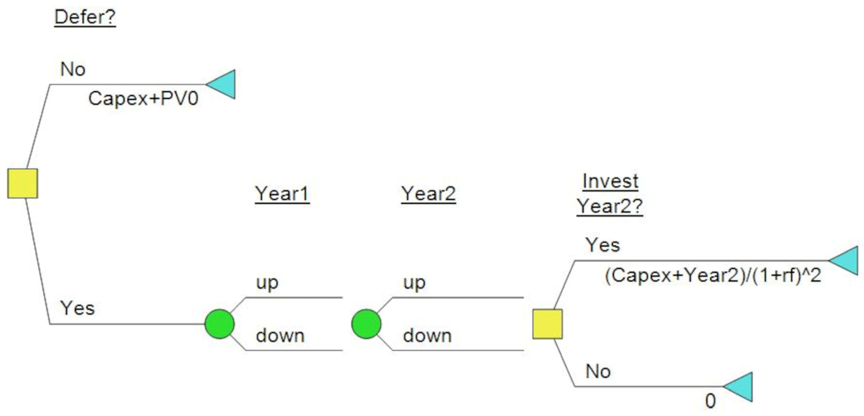
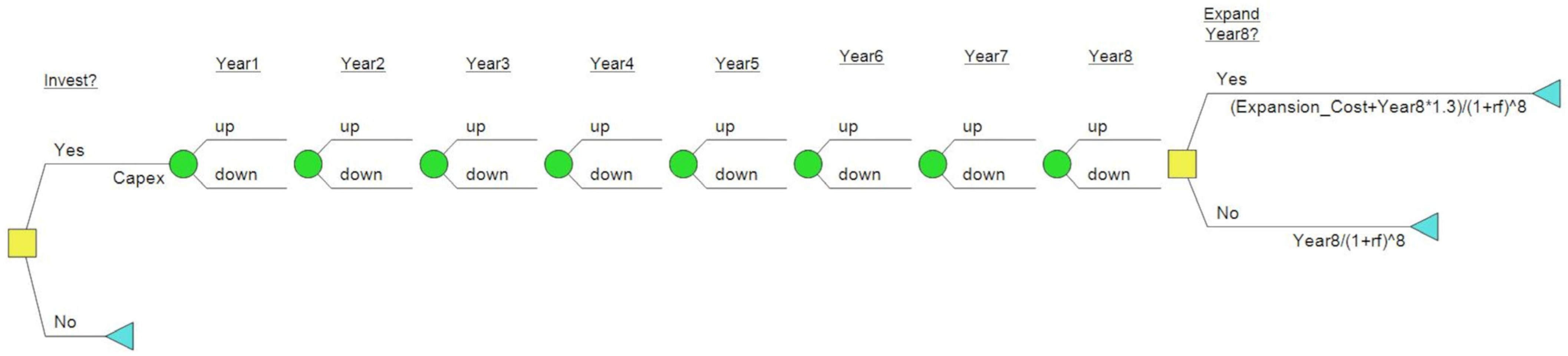
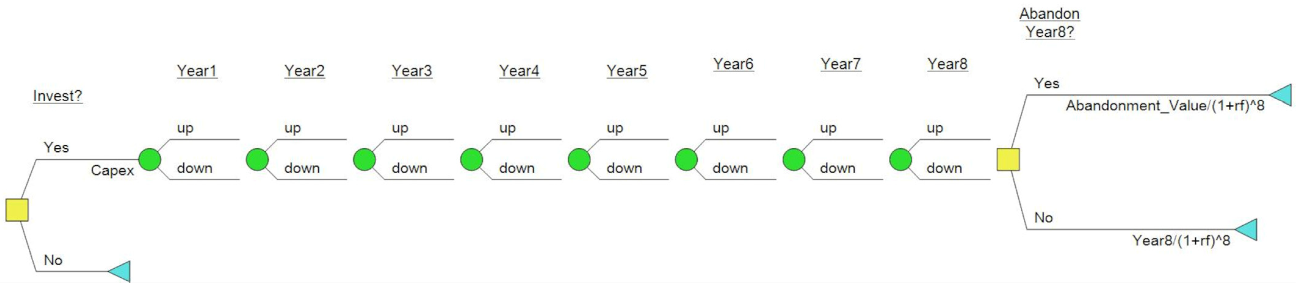
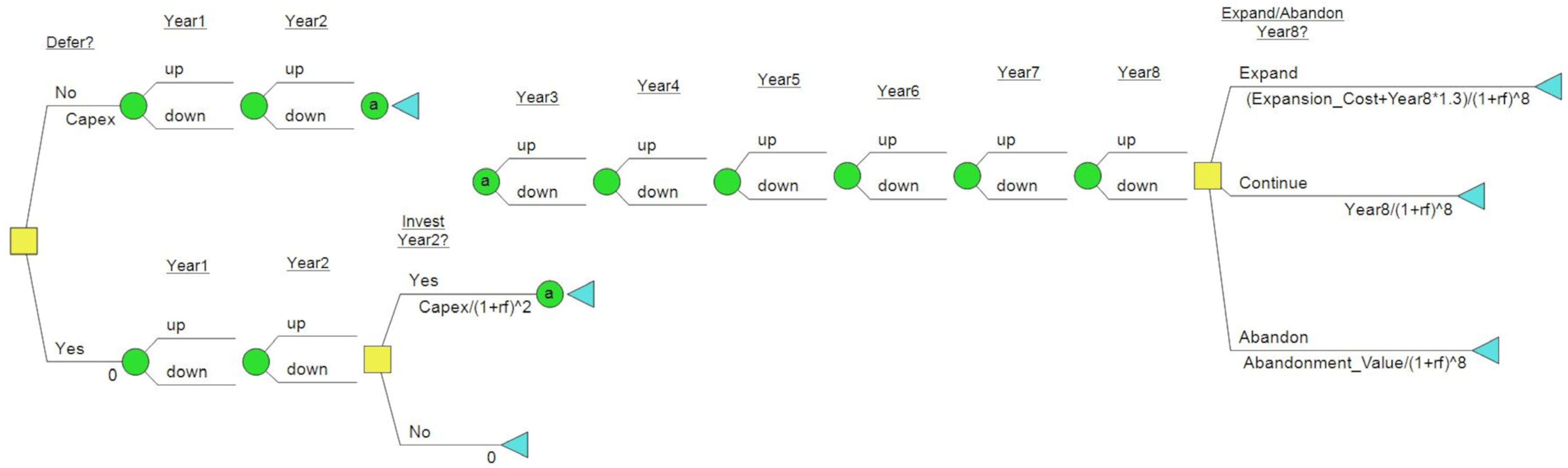
2.3.1. Modeling Investment Projects and Uncertainties

Regarding uncertainties of investment projects, we used three different historical series to model the price of marketed products. The historical series of the tonne price of resin considered monthly data from January 2013 to December 2019 [65]. As for the historical series of standing tree prices from thinning and clearcutting, the frequency was also monthly; however, the period was from June 2017 to July 2019 [66]. Due to the devaluation of the national currency (BRL), we deflated these monetary values to compare and analyze them over time without distortions caused by inflation. According to [67], we remove the effect of nominal value inflation using the General Price Index—Internal Availability. We adopted December 2019 as a new basis for deflated values.

We performed econometric tests on the Napierian logarithm of price returns using the R software [68]. The aim was to establish the stochastic process that best described the future price trajectory of resin time series, thinning, and clearcutting standing.

First, we checked whether the price series were normally distributed using the Jarque–Bera test [69] with a null hypothesis of normal data distribution, using the t series package. Then, we performed the Cox–Stuart test [70] with the null hypothesis that time series did not have a trend, using the randtests package. Through the Dickey–Fuller test [71], with a null hypothesis that the series had a unit root, using the urca package, we analyzed whether the price series were stationary.

We applied the linear regression test to verify whether the price of the historical series in period t − 1 influenced significantly the price in period t. Then, we performed the analysis of residues using the normality test [69] with a null hypothesis of normal data distribution through the t series package.

The three historical series of prices showed characteristics that allowed us to define the geometric Brownian motion (GBM) as the stochastic process for modeling prices. The GBM is a linear first-order stochastic differential equation (SDE) model that consists of a deterministic and a stochastic component [72]. The GBM process described by SDE has an analytical solution using the Itô’s Lemma [73], in which the variable follows a GBM if it satisfies the condition derived from following SDE [74].

$${\mathrm{dP}}_{\mathrm{t}}={\mathsf{\mu }\mathrm{P}}_{\mathrm{t}}\mathrm{dt}+{\mathsf{\sigma }\mathrm{P}}_{\mathrm{t}}{\mathrm{dw}}_{\mathrm{t}}$$

(4)

in which, P_t is the price of the asset at time t, μ is the drift parameter, σ is the standard deviation of the Napierian logarithm of price returns, and dw_t it is the standard increment of a Wiener process.

We adopted the GBM equation, which simulates future prices of assets as a function of asset prices at time t, to model prices of resin and standing trees, according to Equation (5). We determined the stochastic component by the standard normal random variable, ԑ ~ N (0.1).

$${\mathrm{P}}_{\mathrm{t}+1}={\mathrm{P}}_{\mathrm{t}}{\mathrm{e}}^{\left(\mathsf{\mu } -\frac{{\mathsf{\sigma }}^2}{2}\right)\Delta \mathrm{t}+\mathsf{\sigma }\epsilon \sqrt{\Delta \mathrm{t}}}$$

(5)

We obtained the annual volatility from the standard deviation of the Napierian logarithm of price series returns multiplied by $\sqrt{12}$. According to [75], we calculated the drift as a function of annual variance (${\mathsf{\sigma }}^2$) and the annual average of the Napierian logarithm of price series returns ($\overline{\mathrm{z}}$), according to Equation (6).

$$\mathsf{\mu }=\overline{\mathrm{z}}+\frac{{\mathsf{\sigma }}^2}{2}$$

(6)

2.3.2. Volatility of Investment Projects and Risk-Neutral Probabilities of Upward and Downward Movements

We obtained the volatility of investment projects according to [76], which uses the Monte Carlo simulation (MCS) method to estimate the volatility of the project when the underlying asset is the project itself without flexibility.

For this, it was necessary to build stochastic cash flow, that is, to insert uncertainties from resin and standing tree prices and perform MCS. Thus, we considered that the value of the project also followed a GBM. We performed the simulation with the generation of 100,000 iterations, with a fixed initial parameter 12,345, using software @Risk^© 2020 [77], in order to find the probabilistic present value of projects.

Keeping the deterministic present value (${\mathrm{PV}}_0$) constant at the focal date and iterating the stochastic present values (${\mathrm{P}\tilde{\mathrm{V}}}_1$) in the period one, we found the Napierian logarithm of random returns of investment projects, ($\tilde{\mathrm{v}}$), according to Equation (7). As cash flows followed a GBM, the annual volatility of investment projects (σ_p) was given as the standard deviation of random variable $\tilde{\mathrm{v}}$.

$$\tilde{\mathrm{v}}=\ln (\frac{{\mathrm{V}\tilde{\mathrm{P}}}_1}{{\mathrm{VP}}_0})$$

(7)

Thus, we calculated the up (u) and down (d) factors for each node in the binomial tree according to Equations (8) and (9), respectively [78].

$$\mathrm{u}={ \mathrm{e}}^{{\mathsf{\sigma }}_{\mathrm{p}}\sqrt{\Delta \mathrm{t}}}$$

(8)

$$\mathrm{d}=\frac{1}{\mathrm{u}}$$

(9)

The dynamic presents values generated in the binomial tree so that they are discounted at a risk-free rate instead of the risk-adjusted rate. Thus, the risk-neutral probability (Equation (10)) for values of the investment projects goes up (p) and down (1 − p).

$$\mathrm{p}=\frac{\left(1+\mathrm{rf}\right)-\mathrm{d}}{\mathrm{u}-\mathrm{d}}$$

(10)

2.3.3. Binomial Options Pricing Model

According to [79], we build the binomial tree model using DPL decision analysis software [80]. We used the market asset disclaimer (MAD) approach for modeling, so we assumed that the underlying asset was the value of the project without any flexibility [76]. We modeled the investment projects with the management flexibility provided by the application of four different real options models.

First, we analyzed independently the options to defer, expand, and abandon. In this step, we observed the value that each option, individually, added to the investment projects. Subsequently, we analyzed projects with multiple options in the same model, composed of three initial options, to obtain the value attributed to projects when we evaluated the three options combined.

We placed the deferral option for period two of the binomial tree (Figure 1), that is, if the investment was not made at the beginning of the binomial tree, the manager could wait for two years to decide on the investment in case market conditions were more favorable.

We allocated the option to expand the plantation area by 30% and the option to completely abandon the investment projects in period eight of the binomial tree, as it was the moment that the thinning of the forest would happen (Figure 2 and Figure 3). In addition, in case of the abandonment of projects, we obtained a value referring to the sale of the entire forest in the period, added to the sale value of land in the case of the project with land purchase for planting.

The multiple option model (Figure 4) aimed to obtain the value of the options when combined. That way, we offered more options to expand the possible manager decisions.

In order to obtain the real probabilities of the options being exercised, we executed the models using a risk-adjusted rate, that is, the opportunity cost rate of the capital of investment projects, instead of the risk-free rate, according to [81]. We determined the value of real options by maximizing the difference between the value of the underlying asset and the exercise price of the respective option and zero.

Considerations of investments made from the perspective of uncertainties demanded the need to adopt the expanded net present value criterion (ENPV), in order, according to [82,83], to incorporate the additional value related to managerial flexibility. That way, we added ENPV, which was given as the value of real options (ROV) to the traditional net present value (NPV).

3. Results and Discussion

3.1. Deterministic Ecoomic Model

The present value of the land lease project was USD 723, which when added to the project’s CAPEX resulted in a traditional NPV of USD 371. Likewise, the present value of the project that included land purchase was USD 4083, and the NPV was -USD 610.

The investment project with the land lease was viable. However, the investment project with the land purchase was not viable, as the NPV was less than zero since disbursements were not recovered over the life of the project and managers only decide to invest if the project creates value, that is, if the NPV is positive. Therefore, by the traditional analysis of investment based on discounted cash flow, the project with land purchase would be neglected and an investor would look for alternatives with a positive NPV to allocate his capital.

Although the project with the land lease was feasible, it presented a lower present value compared to the project with land purchase, as the annual expenditures were higher due to the cost of the land lease. On the other hand, even with a higher present value, the project with land purchase had a lower NPV since its CAPEX, due to the acquisition of land, was considerably higher than the project with the land lease.

It is noteworthy that a traditional NPV ends to undervalue the value of an investment project, and this makes it unsuitable for risky projects [84,85] and with long planning horizons, as is the case of Pinus elliottii plantations. Thus, when accepting or rejecting investment projects based only on current information and not considering future uncertainties [86,87], inherent in the forest sector, the NPV did not reflect the potential value of the investment projects analyzed.

These weaknesses related mainly to the non-approach to flexibility by the traditional model which can cause inaccurate estimates regarding value generated by cash flows and, consequently, can lead to a devaluation of investment projects [88,89,90].

Thus, the investment project with land purchase should not be immediately discarded, since the value related to managerial flexibility should be accounted for and added to the deterministic value of the project. With this, the manager would have information with values that better represent the potential of projects and, consequently, could make the best decision on whether or not to invest in the projects presented.

3.2. Stochastic Model

In econometric tests for the analysis of the stochastic process, the null hypothesis of normality of data was accepted with a p-value of 0.49, 0.60, and 0.14 for the price historical series of resin, thinning, and clearcutting standing trees, respectively. The null hypothesis that the price series had no trend was rejected, with a p-value of less than 0.05 for the three price series. The null hypothesis that the series had a unit root was rejected, so the price series were non-stationary.

In addition, with the linear regression test, we found that the price was significantly influenced by the price of the exactly previous period. The null hypothesis that residues had a normal distribution was accepted, with a p-value of 0.36, 0.57, and 0.26, for the price of resin, thinning, and clearcutting standing trees, respectively.

Thus, the main characteristics of GBM could be observed in the historical price series analyzed, which supported the choice of GBM as the stochastic process in the price modeling of uncertainties considered in investment projects. We obtained through the MCS the values of 91.25% and 79.87% for the volatility (σ) of the investment project for land purchase and land lease, respectively.

When we conditioned the expectations of the present values from the second to the twenty-first year, the volatility of the projects was characterized by the standard deviation, a measure of dispersion, of the returns of the first year considering the expected values of the following years. From this, the volatility was considered constant throughout the life of the project. Thus, the necessary parameters for building the binomial model were obtained after MCS (

Table 1. Parameters to build the binomial trees.

Parameters	Land Lease	Land Purchase
Volatility (${\mathsf{\sigma }}_{\mathrm{p}}$)	0.7987	0.9125
Up factor ($\mathrm{u}$)	2.2226	2.4906
Down factor ($\mathrm{d}$)	0.4499	0.4015
Risk-neutral probability ($\mathrm{p}$)	0.3409	0.3124
Present value at focal date (${\mathrm{PV}}_0$)	USD 723	USD 4083
CAPEX	USD 352	USD 4693

).

When executing the model with the deferral option, the land lease project showed appreciation, becoming more attractive than the deterministic model when presenting higher ENPV. The land purchase project, previously considered unfeasible because it had an NPV inferior to zero, became viable with the value added by option, since the ENPV was positive (

Table 2. Value of projects with deferral, expansion, and abandonment options.

Real Option	Indicators	Land Lease	Land Purchase
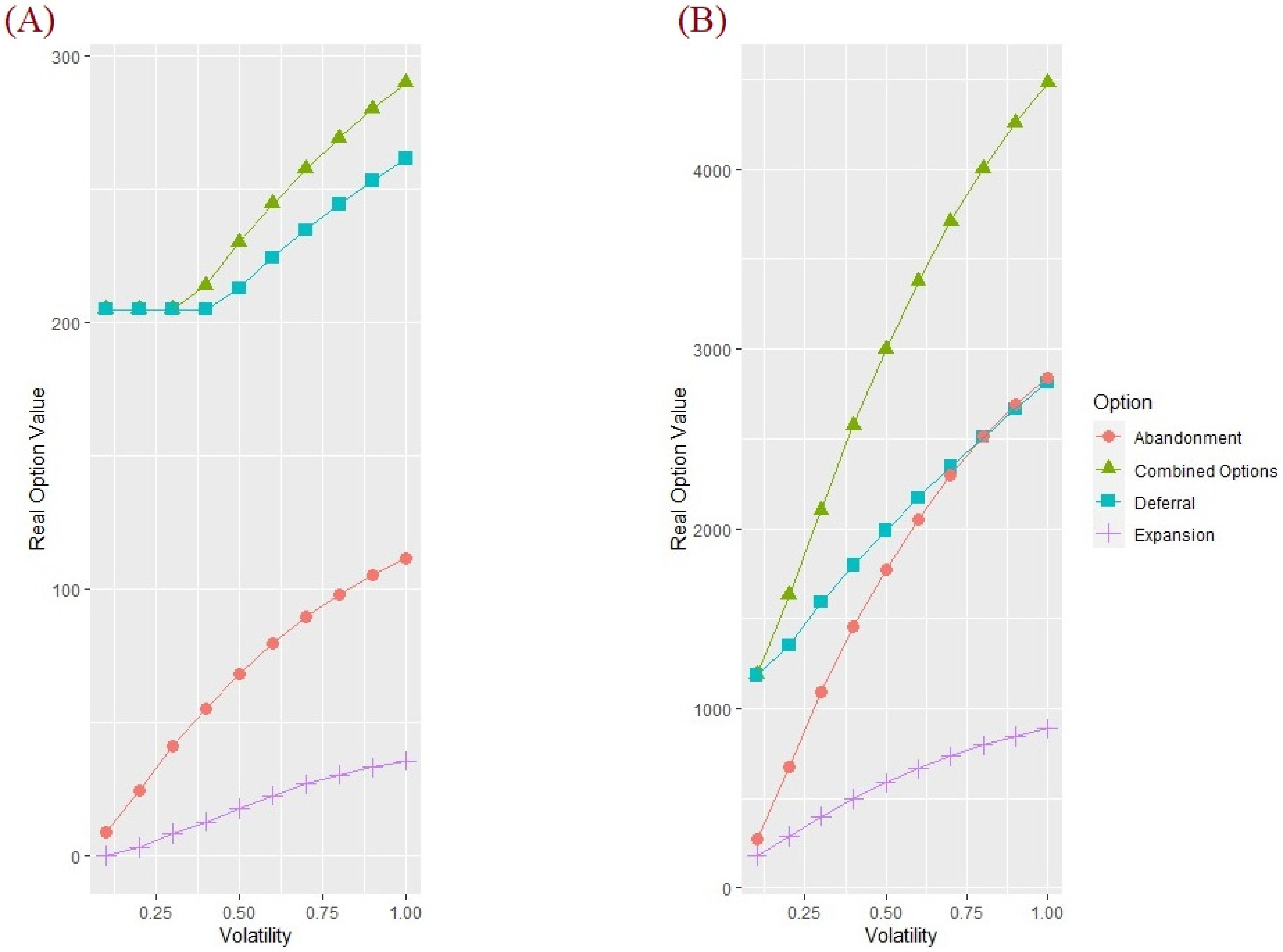
Deferral	ENPV (USD)	486	1812
	Real option value (USD)	115	2422
	Increase in NPV value (%)	31	397
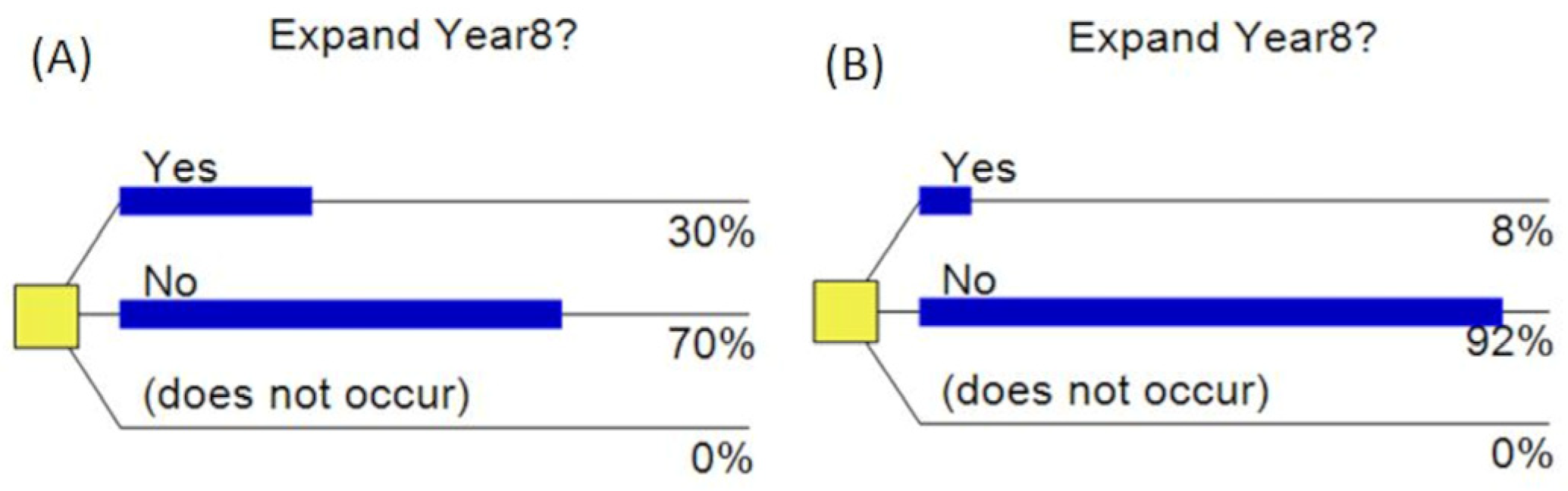
Expansion	ENPV (USD)	559	392
	Real option value (USD)	188	1002
	Increase in NPV value (%)	51	164
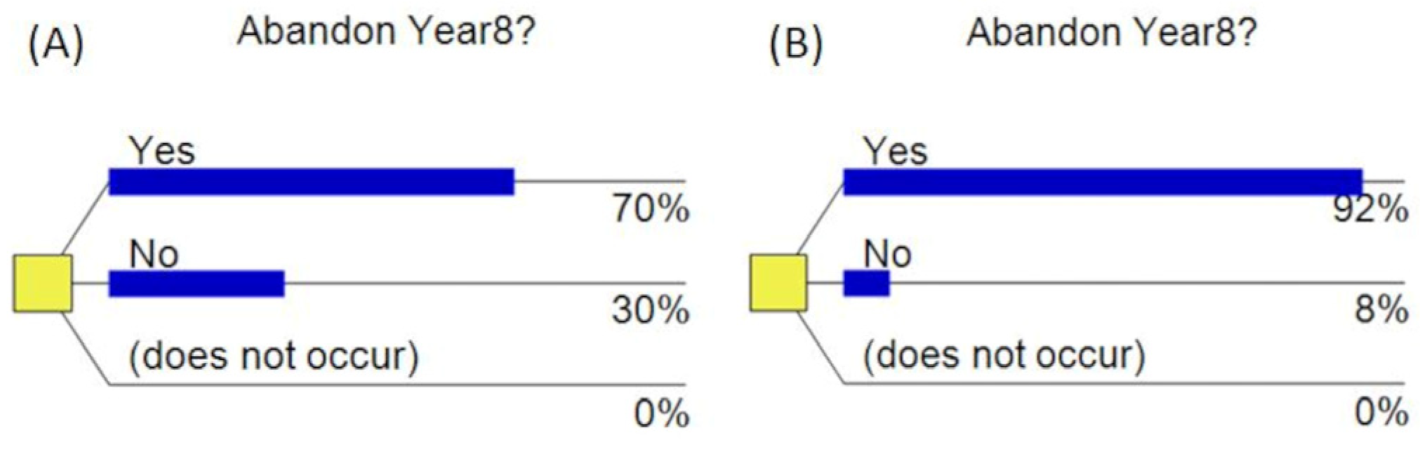
Abandonment	ENPV (USD)	545	1949
	Real option value (USD)	174	2559
	Increase in NPV value (%)	47	420

).

Thus, the premium for the deferral option was higher for the land purchase project and, consequently, the percentage valuation and ENPV were greater. The volatility of the project with purchased land was greater, and according to [91], with increased uncertainty, the option to defer becomes more valuable. This happens because that uncertainty generates a risk premium for waiting to obtain more information, which is the value of the option to defer. According to the authors of [92], this relationship shows that a higher level of uncertainty results in a higher value of deferral option.

In the execution of the binomial model, both investment projects would not be implemented immediately. The option to defer would be exercised, which would postpone the decision to invest for year two of the binomial tree, that is, within the term of the option’s maturity.

When designing an investment, its feasibility will depend on the planning and analysis of financial impacts. When solving expected cash inflows and outflows, it is expected that a well-informed forest manager has an awareness of market risks and fluctuations in projected profitability.

Incorporating the real options analysis into forest investment projects promotes the investor’s perception of risk and managerial flexibility by strategically guiding decision-making. Negotiating the right of deferral does not necessarily impose on the forest manager, when the project is implemented, its feasibility, but rather configures a perspective of opportunity for, if feasible at the time, its assimilation.

The deferral option concatenated to the underlying asset modeled the implementation of the project, aiming to improve profitability by postponing the investment until, according to [93], the emergence of favorable market conditions. Essential in conducting uncertain scenarios, this option provides high quality in management decisions [94,95].

In this period, the greatest probability would be that an investment should occur for the land lease project (Figure 5A), mainly because the project already has a positive NPV. On the other hand, the greatest probability would be that the option was expired, and no investment occurred in the project with land purchase (Figure 5B). As the uncertainty increases, the probability of the project being implemented at that moment decreases [96].

In relation to the land lease investment project, the expansion option was one that added the most value and, consequently, made the project more attractive. The expansion option was one that least contributed to the valuation of the project with land purchase. Despite this, the option added value and made the project viable, as the ENPV was greater than zero (Table 2).

The option to expand the project should only be exercised when the market presents favorable conditions, which allows a greater investment to increase production [97,98]. Thus, the real probability of exercising the expansion option demonstrated that projects should be expanded only in the best scenarios (Figure 6A).

In the project with land purchase, the low probability of exercising the option to expand (8%) explained why valuation was lower compared to the other options (Figure 6B). When indicating non-expansion, it means that the present value of the project’s expected cash flows, if expanded, would not exceed the additional disbursement needed to finance the expansion [99]. This means that when the project has a negative value, it does not obtain any value from the option to expand.

With the expansion option, the forest manager has to allocate a budget to increase link capacities, assuming some cost function with a capacity parameter [100]. The overall costs of expanding capacity are therefore given by the sum of the investment costs. However, as with deferral, managers have the option, but not the obligation, to expand if conditions prove favorable, considering inclusively a management problem due to different cutting and harvesting times.

The abandonment option was one that added the most value to the project with land purchase (Table 2). As the abandonment option is more valuable when residual value is more attractive [101], this higher valuation in the project with land purchase occurred due to the cost of land purchase being recovered when abandoning the project if the scenario was not favorable. On the other hand, the amount spent on leasing land would not recover if the project was abandoned, that is, it was an irreversible cost.

Another reason was the fact that the project with land purchase showed greater volatility. According to the authors of [102], the abandonment option has a more considerable value the greater the uncertainty about the project.

An abandonment option is only exercised if the gain is greater than the present value of expected cash flows until the end of the investment project’s useful life [99]. Thus, real probabilities of the abandonment option being exercised were considerably higher for both investment projects (Figure 7), which demonstrated that, with greater probability, the value generated by projects’ cash flows did not exceed the value of abandoning them.

The value of combined options corresponded to 83% and 72% of the sum of the values of individual options for the projects with lease and purchase of land, respectively. Therefore, the value of the combined options was less than the sum of the values for individual options. According to the authors of [35], the value of multiple options does not normally equal the sum of the same options analyzed individually, as the interactions between the options can be negative or positive and do not occur in a linear way. In addition, interactions depend on a combination of factors, such as type of options (buy or sell), and time separation of their respective exercise dates, among others [103]. Thus, it is imprudent to simply add the values of each real option [104], as the results showed that the interaction between the options analyzed occurred in a negative way.

Although the option values cannot be merely added together, the flexibility of combined options can be significant [105]. When analyzing the three real options together in the model, the options’ value was higher when compared to the real options’ value analyzed individually. With a greater number of choices available through multiple combined real options, managerial flexibility provided to the manager was more expressive [40,106], as shown by the modeling results. Consequently, with more choices available, it was possible to add greater value to the projects, and in effect, increase their attractiveness.

In this way, as well as in the individual options, the project with land purchase was considered viable when it applied the three real options in a combined way (

Table 3. Projects with real options combined.

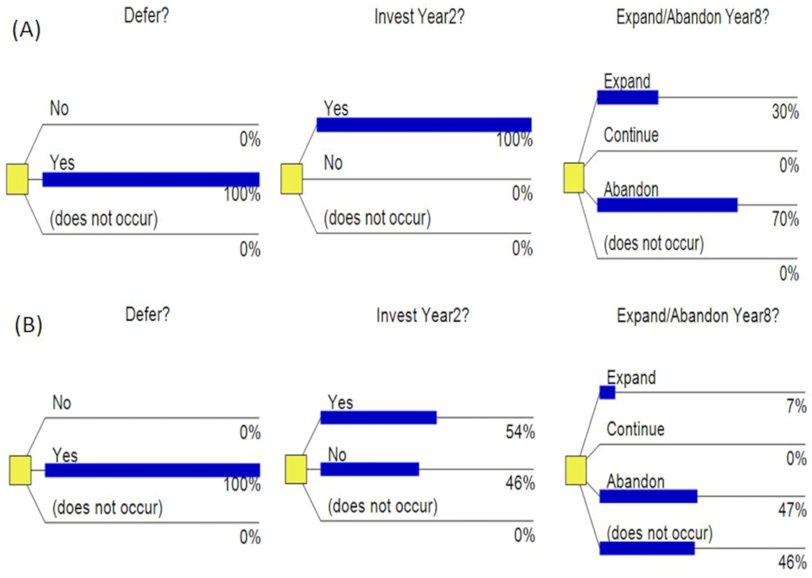
Indicators	Land Lease	Land Purchase
ENPV (USD)	768	3690
Real option value (USD)	397	4300
Increase in NPV value (%)	107	705

). This showed that the value of managerial flexibility, provided by the options’ premium, was responsible for the viability of the project with the land purchase, since this occurred only with the value of the ENPV which represents the stochastic analysis approach.

According to the authors of [81], the flexibility generated by the evaluation model with all the combined options provides a more accurate estimate of the real value of the project as to the isolated options. Thus, the combined options performed better when analyzing investment projects, in which the value of the combined options was equivalent to 35% of the present value of the project with flexibility with land lease, and 51% with land purchase.

Although the project with the land lease was 100% likely to be executed (Figure 8A) and the project with land purchase was 54% (Figure 8B), the percentage increase in value from the traditional NPV to ENPV was considerably higher for the project with land purchase (Table 3).

Therefore, it is possible to affirm that real options had a better influence on the project with land purchase, since it presented a higher traditional present value and volatility, in addition to offering a greater residual value in case of abandonment. Considering the option of abandonment in a planning horizon makes forest managers develop flexible strategies, acting proactively against the uncertainty that impacts investment over the projected horizon.

Managing through the real options analysis means effectively exercising its options, which, in real contexts, are already related without prior planning. Anticipating in the perspective of options trading promotes the redemption of the option premium when the abandonment has the benefit of interrupting operational loss flows, which can be aggravated over time. Even so, maybe after a few years, the market situation could be more favorable again. With strategic alignment, abandonment can be optimized by a temporary stop, until negative flows can be reversed. As they are empirical tasks, the assimilation of the real options analysis needs to be dynamically validated in the provisioning and strategic adequacy exercises.

Thus, although both investment projects are viable in the dynamic model when applying the real options for investment in Pinus elliottii plantations, it is advantageous to choose the project that contemplates the purchase of land, since the ENPV was superior.

As the real options analysis provides a theoretical framework for understanding the impact of uncertainty on irreversible investment [92], the volatility of the project performs a fundamental role in the behavior of value added by the options. That way, it was possible to verify the sensitivity of the real options’ values as to the volatility variation of the project with lease (Figure 9A) and land purchase (Figure 9B).

Therefore, this was as predicted by the option pricing theory, in which greater uncertainty, represented by higher volatility, means higher values for the real option [107,108].

In this way, real options associate uncertainty with flexibility and consider that volatility is the potential value-adding factor to the project [29], as the option values are directly linked to the volatility of underlying asset values [109]. Therefore, real options are favorable in environments with irreversibility and uncertainty [26], characteristics present in investment projects in Pinus elliottii plantations.

By demonstrating that the use of managerial flexibility added value to investment projects and made them more attractive, the application of real options may be of interest to the forest sector. Thus, this research indicates an understanding of the managerial flexibility role and the structure of the real options analysis as a tool capable of providing the potential value of investment projects in Pinus spp. plantations.

4. Conclusions

When applying a real options analysis, individually, the deferral, expansion, and abandonment options add value to investment projects in Pinus elliottii plantations.

The option to expand the forested area is the one that adds the most value to the investment project with land lease. In the investment project with land purchase, this option is abandonment.

Combined real options show the intrinsic financial potential of investment projects in Pinus elliottii plantations, as they simulate the multiple management decisions that can be exercised over a planning horizon.

Investment projects in Pinus elliotti plantations that contemplate the land purchase analyzed through the real options analysis present higher financial returns than those that consider land lease, inverting the result provided by the traditional analysis. Thus, this study contributes to making the real options analysis more accessible to forest managers, allowing it to increase its use in the investment projects of Pinus spp. plantations.

References

- Vihervaara, P.; Marjokorpi, A.; Kumpula, T.; Walls, M.; Kamppinen, M. Ecosystem services of fast-growing tree plantations: A case study on integrating social valuations with land-use changes in Uruguay. For. Policy Econ. 2012, 14, 58–68. [Google Scholar] [CrossRef]
- Brockerhoff, E.G.; Jactel, H.; Parrotta, J.A.; Ferraz, S.F.B. Role of eucalypt and other planted forests in biodiversity conservation and the provision of biodiversity-related ecosystem services. For. Ecol. Manag. 2013, 301, 43–50. [Google Scholar] [CrossRef]
- Marchi, M.; Paletto, A.; Cantiani, P.; Bianchetto, E.; De Meo, I. Comparing Thinning System Effects on Ecosystem Services Provision in Artificial Black Pine (Pinus nigra J. F. Arnold) Forests. Forest 2018, 9, 188. [Google Scholar] [CrossRef] [Green Version]
- Torres, I.; Moreno, J.M.; Morales-Molino, C.; Arianoutsou, M. Ecosystem Services Provided by Pine Forests. In Pines and Their Mixed Forest Ecosystems in the Mediterranean Basin. Managing Forest Ecosystems; Ne’eman, G., Osem, Y., Eds.; Springer: Cham, Switzerland, 2021; pp. 617–629. [Google Scholar]
- Rossato, F.G.F.S.; Susaeta, A.; Adams, D.C.; Hidalgo, I.G.; de Araujo, T.D.; de Queiroz, A. Comparison of revealed comparative advantage indexes with application to trade tendencies of cellulose production from planted forests in Brazil, Canada, China, Sweden, Finland and the United States. For. Policy Econ. 2018, 97, 59–66. [Google Scholar] [CrossRef]
- Brazilian Institute of Geography and Statistics Vegetal Extraction and Forestry Production. Available online: https://biblioteca.ibge.gov.br/visualizacao/periodicos/74/pevs_2020_v35_informativo.pdf (accessed on 20 November 2021).
- Bettinger, P.; Boston, K.; Siry, J.; Grebner, D. Forest Management and Planning; Academic Press: San Diego, CA, USA, 2019. [Google Scholar]
- De Rezende, J.L.P.; de Oliveira, A.D. Análise Econômica e Social de Projetos Florestais; UFV: Viçosa, Brazil, 2008. [Google Scholar]
- Hazra, T.; Samanta, B.; Dey, K. Real option valuation of an Indian iron ore deposit through system dynamics model. Resour. Policy 2019, 60, 288–299. [Google Scholar] [CrossRef]
- Venetsanos, K.; Angelopoulou, P.; Tsoutsos, T. Renewable energy sources project appraisal under uncertainty: The case of wind energy exploitation within a changing energy market environment. Energy Policy 2002, 30, 293–307. [Google Scholar] [CrossRef]
- Yao, J.-S.; Chen, M.-S.; Lin, H.-W. Valuation by using a fuzzy discounted cash flow model. Expert Syst. Appl. 2005, 28, 209–222. [Google Scholar] [CrossRef]
- Berger, R.; Júnior, R.T.; dos Santos, A.J.; Bittencourt, A.M.; de Souza, V.S.; de Loyola Eisfeld, C.; Polz, W.B. Rentabilidade econômica da produção de Pinus spp. por mesorregião homogênea no estado do Paraná. Floresta 2011, 41, 161–168. [Google Scholar] [CrossRef] [Green Version]
- Shogren, J.F. Behavior in forest economics. J. For. Econ. 2007, 12, 233–235. [Google Scholar] [CrossRef]
- Salles, T.T.; Nogueira, D.A.; Beijo, L.A.; da Silva, L.F. Bayesian approach and extreme value theory in economic analysis of forestry projects. For. Policy Econ. 2019, 105, 64–71. [Google Scholar] [CrossRef]
- Feinstein, S.P.; Lander, D.M. A better understanding of why npv undervalues managerial flexibility. Eng. Econ. 2002, 47, 418–435. [Google Scholar] [CrossRef]
- Huchzermeier, A.; Loch, C.H. Project Management Under Risk: Using the Real Options Approach to Evaluate Flexibility in R…D. Manag. Sci. 2001, 47, 85–101. [Google Scholar] [CrossRef]
- Makropoulou, V. Decision tree analysis and real options: A reconciliation. Manag. Decis. Econ. 2011, 32, 261–264. [Google Scholar] [CrossRef]
- Pringles, R.; Olsina, F.; Garcés, F. Designing regulatory frameworks for merchant transmission investments by real options analysis. Energy Policy 2014, 67, 272–280. [Google Scholar] [CrossRef] [Green Version]
- Allen, F.; Bhattacharya, S.; Rajan, R.; Schoar, A. The Contributions of Stewart Myers to the Theory and Practice of Corporate Finance. J. Appl. Corp. Financ. 2008, 20, 8–19. [Google Scholar] [CrossRef]
- Borison, A. Real Options Analysis: Where Are the Emperor’s Clothes? J. Appl. Corp. Financ. 2005, 17, 17–31. [Google Scholar] [CrossRef]
- Kumbaroğlu, G.; Madlener, R.; Demirel, M. A real options evaluation model for the diffusion prospects of new renewable power generation technologies. Energy Econ. 2008, 30, 1882–1908. [Google Scholar] [CrossRef]
- Ford, D.N.; Lander, D.M. Real option perceptions among project managers. Risk Manag. 2011, 13, 122–146. [Google Scholar] [CrossRef]
- Driouchi, T.; Bennett, D.J. Real Options in Management and Organizational Strategy: A Review of Decision-making and Performance Implications. Int. J. Manag. Rev. 2012, 14, 39–62. [Google Scholar] [CrossRef] [Green Version]
- Miller, L.T.; Park, C.S. Decision Making Under Uncertainty—Real Options to the Rescue? Eng. Econ. 2002, 47, 105–150. [Google Scholar] [CrossRef]
- Savolainen, J. Real options in metal mining project valuation: Review of literature. Resour. Policy 2016, 50, 49–65. [Google Scholar] [CrossRef]
- Dyner, I.; Larsen, E.R. From planning to strategy in the electricity industry. Energy Policy 2001, 29, 1145–1154. [Google Scholar] [CrossRef]
- Yin, R. Combining Forest-Level Analysis with Options Valuation Approach—A New Framework for Assessing Forestry Investment. For. Sci. 2001, 47, 475–483. [Google Scholar] [CrossRef]
- Bouchaud, J.; Potters, M. Theory of Financial Risk and Derivative Pricing: From Statistical Physics to Risk Management; Cambridge University Press: Cambridge, UK, 2003. [Google Scholar]
- Santos, L.; Soares, I.; Mendes, C.; Ferreira, P. Real Options versus Traditional Methods to assess Renewable Energy Projects. Renew. Energy 2014, 68, 588–594. [Google Scholar] [CrossRef]
- Ajak, A.D.; Lilford, E.; Topal, E. Real Option Identification Framework for Mine Operational Decision-Making. Nat. Resour. Res. 2019, 28, 409–430. [Google Scholar] [CrossRef]
- Fichman, R.G.; Keil, M.; Tiwana, A. Beyond Valuation: “Options thinking” in IT project management. Calif. Manag. Rev. 2005, 47, 74–96. [Google Scholar] [CrossRef] [Green Version]
- Triantis, A.; Borison, A. Real Options: State of the Practice. J. Appl. Corp. Financ. 2001, 14, 8–24. [Google Scholar] [CrossRef]
- Xiao, Y.; Fu, X.; Oum, T.H.; Yan, J. Modeling airport capacity choice with real options. Transp. Res. Part B Methodol. 2017, 100, 93–114. [Google Scholar] [CrossRef]
- Manfredo, M.R.; Shultz, C.J. Risk, Trade, Recovery, and the Consideration of Real Options: The Imperative Coordination of Policy, Marketing, and Finance in the Wake of Catastrophe. J. Public Policy Mark. 2007, 26, 33–48. [Google Scholar] [CrossRef] [Green Version]
- Trigeorgis, L. The Nature of Option Interactions and the Valuation of Investments with Multiple Real Options. J. Financ. Quant. Anal. 1993, 28, 1–20. [Google Scholar] [CrossRef] [Green Version]
- Lambrecht, B.M. Real options in finance. J. Bank. Financ. 2017, 81, 166–171. [Google Scholar] [CrossRef]
- Cox, J.C.; Ross, S.A.; Rubinstein, M. Option pricing: A simplified approach. J. Financ. Econ. 1979, 7, 229–263. [Google Scholar] [CrossRef]
- Guo, K.; Zhang, L.; Wang, T. Optimal scheme in energy performance contracting under uncertainty: A real option perspective. J. Clean. Prod. 2019, 231, 240–253. [Google Scholar] [CrossRef]
- Herath, H.S.B.; Park, C.S. Multi-stage capital investment opportunities as compound real options. Eng. Econ. 2002, 47, 1–27. [Google Scholar] [CrossRef]
- Ho, S.-H.; Liao, S.-H. A fuzzy real option approach for investment project valuation. Expert Syst. Appl. 2011, 38, 15296–15302. [Google Scholar] [CrossRef]
- Hu, X.; Jie, C. Randomized Binomial Tree and Pricing of American-Style Options. Math. Probl. Eng. 2014, 2014, 291737. [Google Scholar] [CrossRef] [Green Version]
- Bakker, H.; Dunke, F.; Nickel, S. A structuring review on multi-stage optimization under uncertainty: Aligning concepts from theory and practice. Omega 2020, 96, 102080. [Google Scholar] [CrossRef]
- Block, S. Are “Real Options” Actually Used in the Real World? Eng. Econ. 2007, 52, 255–267. [Google Scholar] [CrossRef]
- Čulík, M. Real options valuation with changing volatility. Perspect. Sci. 2016, 7, 10–18. [Google Scholar] [CrossRef] [Green Version]
- Alvares, C.A.; Stape, J.L.; Sentelhas, P.C.; de Moraes Gonçalves, J.L.; Sparovek, G. Köppen’s climate classification map for Brazil. Meteorol. Z. 2013, 22, 711–728. [Google Scholar] [CrossRef]
- Santos, H.G.; Almeida, J.A.; Oliveira, J.B.; Lumbreras, J.F.; Anjos, L.H.C.; Coelho, M.R.; Jacomine, P.K.T.; Cunha, T.J.F.; Oliveira, V.A. Sistema Brasileiro de Classificação de Solos; EMBRAPA: Brasilia, Brazil, 2018. [Google Scholar]
- Nascimento, R.A.; Nunoo, D.B.O.; Bizkarguenaga, E.; Schultes, L.; Zabaleta, I.; Benskin, J.P.; Spanó, S.; Leonel, J. Sulfluramid use in Brazilian agriculture: A source of per- and polyfluoroalkyl substances (PFASs) to the environment. Environ. Pollut. 2018, 242, 1436–1443. [Google Scholar] [CrossRef] [PubMed]
- Deng, Y.; Yang, G.; Xie, Z.; Yu, J.; Jiang, D.; Huang, Z. Effects of Different Weeding Methods on the Biomass of Vegetation and Soil Evaporation in Eucalyptus Plantations. Sustainability 2020, 12, 3669. [Google Scholar] [CrossRef]
- Collet, C.; Vast, F.; Richter, C.; Koller, R. Cultivation profile: A visual evaluation method of soil structure adapted to the analysis of the impacts of mechanical site preparation in forest plantations. Eur. J. For. Res. 2021, 140, 65–76. [Google Scholar] [CrossRef]
- Hevia, A.; Álvarez-González, J.G.; Majada, J. Comparison of pruning effects on tree growth, productivity and dominance of two major timber conifer species. For. Ecol. Manag. 2016, 374, 82–92. [Google Scholar] [CrossRef]
- Dobner, M., Jr.; de Quadros, D.S. Economic Performance of Loblolly Pine Stands in Southern Brazil as a Result of Different Crown Thinning Intensities1. Rev. Árvore 2019, 43, 43. [Google Scholar] [CrossRef]
- Pereira Filho, G.M.; Jacovine, L.A.G.; Schettini, B.L.S.; de Paiva, H.N.; Villanova, P.H.; da Rocha, S.J.S.S.; Leite, H.G. Influence of the Replanting Age on Yield and Growth of Eucalypt Clonal Stands. Rev. Árvore 2020, 44, 2–7. [Google Scholar] [CrossRef]
- Brasil Law No. 9,430, December 27, 1996. Available online: http://www.planalto.gov.br/ccivil_03/LEIS/L9430 (accessed on 17 October 2019).
- Kulakov, N.Y.; Kulakova, A.N. Evaluation of Nonconventional Projects. Eng. Econ. 2013, 58, 137–148. [Google Scholar] [CrossRef]
- Brotherson, W.; Eades, K.; Harris, R.; Higgins, R. “Best Practices” in Estimating the Cost of Capital: An Update. J. Appl. Financ. 2013, 23, 1–19. [Google Scholar]
- Moody’s Rating Country Default Spreads. Available online: https://www.moodys.com/credit-ratings/Brazil-Government-of-credit-rating-114650 (accessed on 17 October 2019).
- Baker, H.K.; English, P. Capital Budgeting Valuation: Financial Analysis for Today’s Investment Projects; John Wiley & Sons: Hoboken, NJ, USA, 2011. [Google Scholar]
- Department of the Treasury T-Bonds. Available online: https://www.treasury.gov/resource-center/data-chart-center/interest-rates/Pages/TextView.aspx?data=yieldAll (accessed on 17 October 2019).
- Viebig, J.; Poddig, T.; Varmaz, A. Equity Valuation: Models from Leading Investment Banks; John Wiley & Sons: Chichester, UK, 2008. [Google Scholar]
- Bowman, R.G.; Bush, S.R. Using Comparable Companies to Estimate the Betas of Private Companies. J. Appl. Financ. 2006, 16, 71–82. [Google Scholar]
- Brasil, Bolsa, B. Cotações Históricas. Available online: http://www.b3.com.br/pt_br/market-data-e-indices/servicos-de-dados/market-data/historico/mercado-a-vista/cotacoes-historicas (accessed on 17 December 2019).
- S&P Down Jones S&P Global Timber & Forestry Index. Available online: https://www.spglobal.com/spdji/en/indices/equity/sp-global-timber-and-forestry-index/#overview (accessed on 17 December 2019).
- Institute for Applied Economic Research Emerging Markets Bond Index + Risco Brasil (EMBI + RB). Available online: http://www.ipeadata.gov.br/ExibeSerie.aspx?serid=40940&module=M (accessed on 15 December 2019).
- Damodaran, A. The Dark Side of Valuation: Valuing Young, Distressed, and Complex Businesses; Pearson Education: Upper Saddle River, NJ, USA, 2010. [Google Scholar]
- Aresb Average Price of Resin. Available online: http://www.aresb.com.br/portal/preco-medio-resina (accessed on 17 November 2021).
- Cepa Monthly Agricultural Prices. Available online: https://cepa.epagri.sc.gov.br/index.php/produtos/mercado-agricola/precos-agricolas-mensais-indice (accessed on 17 November 2021).
- Mendes, J.T.G.; Padilha Junior, J.B. Agronegócio: Uma Abordagem Econômica; Pearson Prentice Hall: São Paulo, Brizal, 2007. [Google Scholar]
- Team, R.D.C. RStudio: A Language and Environment for Statistical Computing; RStudio: Boston, MA, USA, 2020. [Google Scholar]
- Jarque, C.M.; Bera, A.K. Efficient tests for normality, homoscedasticity and serial independence of regression residuals. Econ. Lett. 1980, 6, 255–259. [Google Scholar] [CrossRef]
- Cox, D.R.; Stuart, A. Some Quick Sign Tests for Trend in Location and Dispersion. Biometrika 1955, 42, 80–95. [Google Scholar] [CrossRef] [Green Version]
- Dickey, D.A.; Fuller, W.A. Distribution of the Estimators for Autoregressive Time Series with a Unit Root. J. Am. Stat. Assoc. 1979, 74, 427–431. [Google Scholar] [CrossRef]
- Ossenbruggen, P.J.; Laflamme, E.M. Explaining Freeway Breakdown with Geometric Brownian Motion Model. J. Transp. Eng. Part A Syst. 2019, 145, 4019037. [Google Scholar] [CrossRef]
- Maeda, M.; Watts, D. The unnoticed impact of long-term cost information on wind farms’ economic value in the USA—A real option analysis. Appl. Energy 2019, 241, 540–547. [Google Scholar] [CrossRef]
- Rębiasz, B. The valuation of real options in a hybrid environment. Oper. Res. Decis. 2019, 29, 97–119. [Google Scholar] [CrossRef]
- Insley, M. A Real Options Approach to the Valuation of a Forestry Investment. J. Environ. Econ. Manag. 2002, 44, 471–492. [Google Scholar] [CrossRef]
- Copeland, T.E.; Antikarov, V. Opções Reais: Um novo Paradigma para Reinventar a Avaliação de Investimentos; Campus Verlag: Rio de Janeiro, Brizal, 2001. [Google Scholar]
- Palisade Corporation @Risk Versão 8.0 Ithaca. Available online: https://www.palisade-br.com (accessed on 15 May 2020).
- Kim, K.; Park, H.; Kim, H. Real options analysis for renewable energy investment decisions in developing countries. Renew. Sustain. Energy Rev. 2017, 75, 918–926. [Google Scholar] [CrossRef]
- Brandão, L.E.; Dyer, J.S.; Hahn, W.J. Using Binomial Decision Trees to Solve Real-Option Valuation Problems. Decis. Anal. 2005, 2, 69–88. [Google Scholar] [CrossRef]
- Dalton, C.; Manzella, T.; Franz, N. Syncopation DPL: Decision Programming Language 2020; Syncopation: Concord, MA, USA, 2020. [Google Scholar]
- Miranda, O.; Brandão, L.E.; Lazo, J.L. A dynamic model for valuing flexible mining exploration projects under uncertainty. Resour. Policy 2017, 52, 393–404. [Google Scholar] [CrossRef]
- Mun, J. Real Options Analysis: Tools and Techniques for Valuing Strategic Investments and Decisions; John Wiley & Sons: Hoboken, NJ, USA, 2006. [Google Scholar]
- Trigeorgis, L. Making use of real options simple: An overview and applications in flexible/modular decision making. Eng. Econ. 2005, 50, 25–53. [Google Scholar] [CrossRef]
- Dimitrakopoulos, R.G.; Sabour, S.A.A. Evaluating mine plans under uncertainty: Can the real options make a difference? Resour. Policy 2007, 32, 116–125. [Google Scholar] [CrossRef]
- Lee, I.; Lee, K. The Internet of Things (IoT): Applications, investments, and challenges for enterprises. Bus. Horiz. 2015, 58, 431–440. [Google Scholar] [CrossRef]
- Liu, X.; Ronn, E.I. Using the binomial model for the valuation of real options in computing optimal subsidies for Chinese renewable energy investments. Energy Econ. 2020, 87, 104692. [Google Scholar] [CrossRef] [Green Version]
- Suttinon, P.; Nasu, S. Real Options for Increasing Value in Industrial Water Infrastructure. Water Resour. Manag. 2010, 24, 2881–2892. [Google Scholar] [CrossRef]
- Boomsma, T.K.; Meade, N.; Fleten, S.-E. Renewable energy investments under different support schemes: A real options approach. Eur. J. Oper. Res. 2012, 220, 225–237. [Google Scholar] [CrossRef]
- Martínez-Ceseña, E.A.; Mutale, J. Application of an advanced real options approach for renewable energy generation projects planning. Renew. Sustain. Energy Rev. 2011, 15, 2087–2094. [Google Scholar] [CrossRef]
- Shaffie, S.S.; Jaaman, S.H. Monte Carlo on Net Present Value for Capital Investment in Malaysia. Procedia-Soc. Behav. Sci. 2016, 219, 688–693. [Google Scholar] [CrossRef] [Green Version]
- Benaroch, M.; Kauffman, R.J. A Case for Using Real Options Pricing Analysis to Evaluate Information Technology Project Investments. Inf. Syst. Res. 1999, 10, 70–86. [Google Scholar] [CrossRef] [Green Version]
- Golub, A.A.; Lubowski, R.N.; Piris-Cabezas, P. Business responses to climate policy uncertainty: Theoretical analysis of a twin deferral strategy and the risk-adjusted price of carbon. Energy 2020, 205, 117996. [Google Scholar] [CrossRef]
- Cardin, M.-A.; Zhang, S.; Nuttall, W.J. Strategic real option and flexibility analysis for nuclear power plants considering uncertainty in electricity demand and public acceptance. Energy Econ. 2017, 64, 226–237. [Google Scholar] [CrossRef] [Green Version]
- Cardin, M.-A. Enabling Flexibility in Engineering Systems: A Taxonomy of Procedures and a Design Framework. J. Mech. Des. 2014, 136, 011005. [Google Scholar] [CrossRef] [Green Version]
- Sabri, Y.; Hadi, P.O.; Hariyanto, N. Decision Area of Distributed Generation Investment as Deferral Option in Industrial Distribution System Using Real Option Valuation. Int. J. Electr. Eng. Inform. 2016, 8, 1. [Google Scholar] [CrossRef]
- Folta, T.B.; Johnson, D.R.; O’Brien, J. Uncertainty, irreversibility, and the likelihood of entry: An empirical assessment of the option to defer. J. Econ. Behav. Organ. 2006, 61, 432–452. [Google Scholar] [CrossRef]
- Arango, M.A.A.; Cataño, E.T.A.; Hernández, J.D. Valoración de proyectos de energía térmica bajo condiciones de incertidumbre a través de opciones reales. Rev. Ing. Univ. Medellín 1970, 12. [Google Scholar] [CrossRef] [Green Version]
- Guo, K.; Zhang, L. Guarantee optimization in energy performance contracting with real option analysis. J. Clean. Prod. 2020, 258, 120908. [Google Scholar] [CrossRef]
- Durica, M.; Guttenova, D.; Pinda, L.; Svabova, L. Sustainable Value of Investment in Real Estate: Real Options Approach. Sustainability 2018, 10, 4665. [Google Scholar] [CrossRef] [Green Version]
- Chow, J.Y.J.; Regan, A.C. Network-based real option models. Transp. Res. Part B Methodol. 2011, 45, 682–695. [Google Scholar] [CrossRef]
- Arya, A.; Glover, J. Abandonment Options and Information System Design. Rev. Account. Stud. 2003, 8, 29–45. [Google Scholar] [CrossRef]
- Damaraju, N.L.; Barney, J.B.; Makhija, A.K. Real options in divestment alternatives. Strateg. Manag. J. 2015, 36, 728–744. [Google Scholar] [CrossRef]
- Bowe, M.; Lee, D.L. Project evaluation in the presence of multiple embedded real options: Evidence from the Taiwan High-Speed Rail Project. J. Asian Econ. 2004, 15, 71–98. [Google Scholar] [CrossRef]
- Schachter, J.A.; Mancarella, P. A critical review of Real Options thinking for valuing investment flexibility in Smart Grids and low carbon energy systems. Renew. Sustain. Energy Rev. 2016, 56, 261–271. [Google Scholar] [CrossRef]
- Duku-Kaakyire, A.; Nanang, D.M. Application of real options theory to forestry investment analysis. For. Policy Econ. 2004, 6, 539–552. [Google Scholar] [CrossRef]
- Shuiabi, E.; Thomson, V.; Bhuiyan, N. Entropy as a measure of operational flexibility. Eur. J. Oper. Res. 2005, 165, 696–707. [Google Scholar] [CrossRef]
- Bayram, K.; Ganikhodjaev, N. On pricing futures options on random binomial tree. J. Phys. Conf. Ser. 2013, 435, 12043. [Google Scholar] [CrossRef] [Green Version]
- Bøckman, T.; Fleten, S.-E.; Juliussen, E.; Langhammer, H.J.; Revdal, I. Investment timing and optimal capacity choice for small hydropower projects. Eur. J. Oper. Res. 2008, 190, 255–267. [Google Scholar] [CrossRef] [Green Version]
- Fleten, S.-E.; Gunnerud, V.; Hem, Ø.; Svendsen, A. Real Option Valuation of Offshore Petroleum Field Tie-ins. J. Real Options 2011, 1, 1–17. [Google Scholar]