Stand Volume Growth Modeling with Mixed-Effects Models and Quantile Regressions for Major Forest Types in the Eastern Daxing’an Mountains, Northeast China

Abstract

The relative growth rate ($RG{R}_{nv}$) is the standardized measurement of forest growth, whereby excluding the size differences between individuals allows their performance to be compared equally. The $RG{R}_{nv}$ model was developed using the National Forest Inventory ($\mathrm{NFI}$) data on the Daxing’an Mountains, in Northeast China, which contain Dahurian larch (Larix gmelinii Rupr.), white birch (Betula platyphylla Suk.), and mixed coniferous–broadleaf forests. Four predictor variables—i.e., quadratic mean diameter ($D_q$), stand basal area ($G$), average tree height ($H_a$), and altitude ($A$)—and four different methods—i.e., the nonlinear mixed-effects models ($\mathrm{NLME}$), three nonlinear quantile regression ($\mathrm{NQR}3$), five nonlinear quantile regression ($\mathrm{NQR}5$), and nine nonlinear quantile regression ($\mathrm{NQR}9$) models—were used in this study. All the models were validated using the leave-one-out method. The results showed that (1) the mixed coniferous–broadleaf forest presented the highest $RG{R}_{nv}$; (2) the $RG{R}_{nv}$ was negatively correlated with the four predictors, and the heteroscedasticity reduced significantly after the weighting function was integrated into the models; and (3) the quantile regression models performed better than $\mathrm{NLME}$, and $\mathrm{NQR}9$ outperformed both $\mathrm{NQR}3$ and $\mathrm{NQR}5$. To make more accurate predictions, parameters of the adjusted mixed-effects and quantile regression models should be recalculated and localized using sampled $RG{R}_{nv}$ in each region and then applied to predict all the other $RG{R}_{nv}$ of plots. $MAPE\left(\%\right)$ indicates the mean absolute percentage error. The values were stable when the sample numbers were greater than or equal to six across the three forest types, which showed relatively accurate and lowest-cost prediction results.

1. Introduction

Forests represent the habitat for most of the earth’s terrestrial biodiversity, occupying almost 4.06 billion ha or 31% of the earth’s total land area. Deforestation and forest degradation are two reasons for the decrease in forest area, which has been lost at an alarming rate of 4.7 million ha per year during 2010–2020 [1]. Consequently, China has gradually banned the commercial logging of natural forests in the eastern Daxing’an Mountains since 2015 to recover the natural forests. This ban has been successfully implemented with the current total volume of 547 million m³ or about 92.01% of the total natural potential of the eastern Daxing’an forest [2]. However, many natural forests with no production demand need a new management plan to specifically address more appropriate and effective monitoring and adjustment methods to ensure their continuity. One of the most effective ways is to monitor and update real-time forest growth, which significantly impacts forest structure and composition over time [3]. Unfortunately, to the best of the authors’ knowledge, no research has been found regarding the forest growth model in the eastern Daxing’an Mountains.

Forest growth is defined as the size of a tree or a stand produced within a certain period [4]. Forest growth and yield research has provided forest managers with an abundance of tools for simulating stand dynamics [5]. This research was begun in the 1850s in Central Europe when the basic yield tables became the primary standard for growth and yield estimation until the 1950s [6]. The basic yield tables might be helpful in actual application; however, their low accuracy is gradually becoming unacceptable to both academicians and practitioners. Hence, the mathematical–statistical analysis and modeling of forest growth have been increasingly developed to fulfill the demand for more accurate estimation. As a result, numerous classic functions can be used to better estimate forest growth, such as those of Chapman–Richards, Kangas, Monomolecular, Weibull, and Korf [7,8,9].

However, the growth function is not suitable for the uneven forest, because of the difficulty in determining the age of many natural forests [10]. Moser and Hall [11] proposed a function of a measurable size characteristics of the stand under investigation to eliminate the problem of indefinite age. This growth rate equation provides a yield function expressed with an elapsed time from a given initial condition, indicating that compatible growth rate and yield functions for the uneven-aged stand can be derived from permanent plot data. Dale et al. [12] classified growth and yield models into stand model, size class model, and individual tree model. Peng [13] detailed the differences between these three models: stand models use stand parameters to simulate the stand growth and yield that are usually simple and robust; however, they provide little or no detail about individual trees within a stand; size class models only require overall stand values as input and provide some information relating to stand structure, but the output is not flexible enough to evaluate a broad range of stand treatments; and the individual tree models simulate each individual tree as a basic unit that provides maximum detail and flexibility for evaluating the stand but requires more detail and an expensive database to be developed and implemented. Although the stand models cannot provide specific information about the individual tree or size class, it is generally cheaper and relatively effective for practical applications because of lesser data and the need for complex variables [14].

There are several different basic concepts of growth, which have not been properly explained and often appear confusing. Cumulative growth means the total volume attained by a tree or a stand at any particular time. Generally, cumulative growth time is a fixed interval, which is not convenient for practical application. Absolute growth rate ($AG{R}_{nv}$) is the mean absolute changes in mass over a given time period, which can be defined as the value of a particular characteristic at different times ($t_k$ and $t_{k-1}$ divided by $\Delta t$). $AG{R}_{nv}$ depends on the current state of the plant size characteristic and is therefore not helpful to growth analysts when comparing plants of different sizes [15]. In such situations, $RG{R}_{nv}$ is often studied in addition to absolute growth. $RG{R}_{nv}$ is also a function of time and is defined as the increase in size relative to the growth characteristic [3]. Hunt [7] decomposed $RG{R}_{nv}$ into the product of three components: (1) the net assimilation rate ($NAR$), which is the absolute growth rate per unit leaf area; (2) the leaf mass ratio ($LMR$), which is the proportion of biomass invested in leaves; and (3) the specific leaf area ($SLA$), which is the leaf area divided by leaf mass. Given the advantages of $\mathrm{RGR}$ in physiology and ecology, it was used in this study as the dependent variable.

Permanent plot data from different regions are mostly used for forest growth modeling. However, heteroscedasticity always exists in model residuals; hence, a weighted regression should be used to neutralize the inconsistency [16,17]. The traditional ordinary least-squares ($\mathrm{OLS}$) method obeys the assumption of independent observations, providing the proper parameter estimates for the overall average. However, their variances are biased when there are significant differences between groups. Since the measured trees or stands are usually grouped into plots or regions, the nonlinear mixed-effects ($\mathrm{NLME}$) modeling approach has been used to reduce the bias by considering the differences between groups [18,19,20,21]. The $\mathrm{NLME}$ is composed of fixed- and random-effects parameters, in which the variance–covariance structure analyzes hierarchically structured data more efficiently and subsequently increases the prediction accuracy of the models. $\mathrm{NQR}$ has been widely used in the last few years to describe the response variable, given a set of explanatory variables [22,23,24]. Compared to the conventional $\mathrm{OLS}$ method, quantile regression can characterize the entire conditional distribution of the outcome variable and is more robust to the presence of outliers and misspecification of the error distribution [25]. However, in actual application, both the $\mathrm{NLME}$ and $\mathrm{NQR}$ should be calibrated for the adjusted random parameters and the best quantile curve [26,27,28].

The main research tasks of this study were to (i) choose the best basic model equation for $RG{R}_{nv}$ and solve model autocorrelation and heterogeneity using the $\mathrm{NLME}$ and $\mathrm{NQR}$ methods; (ii) evaluate different $RG{R}_{nv}$ models using a leave-one-out cross-validation approach and compare the $RG{R}_{nv}$ of three forest types and analyze the trend differences between mixed and relatively pure stands; and (iii) determine an appropriate sample size that considers both sample cost and predictive accuracy. The finding will be useful in forest management planning for the uneven-aged forests in the eastern Daxing’an Mountains. It will also expand the application of mixed-effects and quantile regression models in stand growth modeling, which will be useful in effectively estimating the dynamics of future forest accumulation and providing a theoretical basis for carbon neutrality. Continuously improving our understanding of $RG{R}_{nv}$ impacts on the comparison of pure and mixed forests will support forest managers seeking to develop effective adaptation measures and determine sustainable forestry production.

2. Materials and Methods

2.1. Study Sites

We selected the eastern Daxing’an Mountains located in Heilongjiang Province, Northeast China (50°05′–55°33′ N, and 121°11′–127°01′ E). It is the largest and best-preserved natural forest in China (Figure 1), covering approximately 6.62 million ha (97.46% of the total forest area), with a total volume of living trees of about 540 million m³ (98.72% of the total forest volume). The average width is approximately 200 km, stretching 1200 km from northeast to southwest. The altitude ranges from 300 to 1520 m above the sea level. This area belongs to the typical cold temperate continental monsoon climate, with mean annual temperature and total precipitation ranging from −1 to −2.8 °C and 430 to 460 mm, respectively. The soils are mostly cryumbrepts or humic cambisols (or brown coniferous forest soils in the Chinese taxonomic system) [29,30]. The main dominant tree species are Dahurian larch (Larix gmelinii Rupr.) and white birch (Betula platyphylla Suk.), accompanied by Dahurian poplar (Populus davidiana Dode.), Mongolian oak (Quercus mongolica), and Mongolian pine (Pinus sylvestris var. mongolica). There are three main forest types in the eastern Daxing’an Mountains: LF, WBF, and CBMF. The areas of the three main forest types are 2.54 million (37.39% of the total forest area), 2.23 million hectares (32.83% of the total forest area), and 0.69 million hectares (10.16% of the total forest area), respectively.

Figure 1. The geographical position of the study area and the forest bureaus (regions) in eastern Daxing’an Mountains, Northeast China.

2.2. Modeling Data

$\mathrm{NFI}$ data are network representatives designed to continuously monitor the macro-changes of forest resources at the national and provincial levels at 5 years. The main objectives of the $\mathrm{NFI}$ are to identify the forest extent, such as volume, growth, consumption, function, and dynamics during each interval. In eastern Daxing’an Mountains, the $\mathrm{NFI}$ sampling design is an 8 km × 8 km grid, and a permanent sampling plot is located at every grid.

Measurements that were used in this study came from 384 permanent $\mathrm{NFI}$ plots. These plots were located in 12 forest bureaus (or 12 regions), which covered most of the eastern Daxing’an Mountain area. The data were collected in three periods of 2000–2005, 2005–2010, and 2010–2015, respectively, with a total of 1152 samples investigated. The data represented three main natural forest types in the eastern Daxing’an Mountains, comprising $\mathrm{LF}$, $\mathrm{WBF}$, and $\mathrm{CBMF}$ (dominated by the intermixture of Dahurian larch and white birch). The rectangular plots had a size of 10 × 60 m, which was equal to 0.06 ha. No logging or human intervention was detected within the sample plots. All trees with diameter at breast height greater than 5 cm were measured, and information including the species name, $\mathrm{DBH}$, tree status, and number of trees per sample plot was collected. For each plot, the heights of 3–5 standard trees (determined by the $D_q$) for the dominant species in a plot were measured using a Blume–Leiss hypsometer to calculate the mean height of these trees as $H_a$. The stand basal area was calculated with Equation (1). Individual tree volume was calculated with the one-way volume table for each forest bureau based on the diameter at breast height, and the system error is within $\pm 1\%$ [31]. The stand volume was calculated with Equation (2). The Pressler growth rate formula, Equation (3), was used to calculate the $RG{R}_{nv}$, in which the periodic average growth rate was substituted for the instantaneous growth rate [32]. The abbreviations for the main variables and terms involved in the article are shown in Table 1. The descriptive statistics of the stand variables are provided in Table 2.

$$G_j=\raisebox{1ex}{${{\displaystyle \sum }}_i^k\frac{\mathsf{\pi }{D}_i{}^2}{40000}$}\!\left/ \!\raisebox{-1ex}{$\mathrm{Area}$}\right.$$

(1)

$$V_i=\raisebox{1ex}{${{\displaystyle \sum }}_i^k\frac{v_i}{40000}$}\!\left/ \!\raisebox{-1ex}{$\mathrm{Area}$}\right.$$

(2)

$$RG{R}_{nv}=\frac{V_{i_t}-V_{i_{t-n}}}{V_{i_t}+V_{i_{t-n}}}\times \frac{200}{\mathrm{n}}$$

(3)

where $V_{i_{t-n}}$ and $V_{i_t}$ represent the initial and final stand volume of $i$th plot, respectively, which are equivalent to the accumulation of the live stand volume, ingrowth volume, and harvest volume; $k$ represents the numbers of plot; n represents the investigation interval in Equation (3).

Table 1. Descriptions of the main variables and terms for the three forest types in the eastern Daxing’an Mountains, Northeast China.

Abbreviation	Description
Stand variables
$A$ (m)	Altitude of plot
$D_d$ (cm)	Mean diameter of dominant species
$D_q$ (cm)	Quadratic mean diameter of the dominant species
$G$ (m2·ha−1)	Stand basal area
$H_a$ (m)	Mean height of dominant species
$N$ (trees·ha−1)	Number of trees per hectare
$RG{R}_{nv}$	Relative growth rate
$S$ (°)	Slope of the plot
$V$ (m3·ha−1)	Volume of the plot
Proper noun
BASIC	Basic nonlinear model
$\mathrm{CBMF}$	Mixed coniferous–broadleaf forests
FIXED	Fixed-effects model
$\mathrm{LF}$	Dahurian larch (Larix gmelinii Rupr.) forest
$NFI$	The National Forest Inventory data
$\mathrm{NLME}/\mathrm{MIXED}$	Nonlinear mixed-effects model
$\mathrm{NQR}$(3, 5, 9)	Nonlinear quantile regression model(3, 5, 9 quantile points)
$\mathrm{WBF}$	White birch (Betula platyphylla Suk.)
Statistics index
$\mathrm{AIC}$	Akaike information criterion
$MAE$	Mean absolute error
$MAPE\left(\%\right)$	Mean absolute percent error
$MPE\left(\%\right)$	Mean percent error
$R_a^2$	Adjusted coefficient of determination
$\mathrm{RMSE}$	Root mean square error

Table 2. Descriptive statistics of variables of the three forest types in the eastern Daxing’an Mountains, Northeast China.

Forest Type	Variable	Sample Sizes	Mean	Min.	Max.	S.D.
$\mathrm{LF}$ (N = 151)	$A$ (m)	453	634.83	220	1190	206.75
	$D_d$ (cm)	453	14.51	6.91	40.23	5.33
	$D_q$ (cm)	453	12.84	5.21	29.71	3.36
	$G$(m2·ha−1)	453	13.16	1.51	35.09	7.48
	$H_a$ (m)	453	13.25	4.13	24.71	3.67
	$N$(trees·ha−1)	453	1094	117	3950	695
	$S$ (°)	453	6.15	0.00	28.00	5.07
	$V$ (m3·ha−1)	453	86.74	7.21	288.82	53.21
	$RG{R}_{nv}$ (%·year−1)	453	2.68	0.13	11.25	1.86
$\mathrm{WBF}$ (N = 101)	$A$ (m)	303	628.13	241	1150	184.21
	$D_d$ (cm)	303	11.54	6.19	22.12	2.56
	$D_q$ (cm)	303	11.21	5.12	21.52	2.63
	$G$ (m2·ha−1)	303	12.45	1.63	26.36	5.19
	$H_a$ (m)	303	12.19	5.41	20.61	2.64
	$N$ (trees·ha−1)	303	1332	167	3350	664
	$S$ (°)	303	6.94	0.00	26.00	4.71
	$V$ (m3·ha−1)	303	74.89	7.81	170.01	34.51
	$RG{R}_{nv}$ (%·year−1)	303	3.13	0.41	9.59	1.65
$\mathrm{CBMF}$ (N = 132)	$A$ (m)	396	601.83	235	1050	189.01
	$D_d$ (cm)	396	13.51	6.22	46.51	4.61
	$D_q$ (cm)	396	12.19	5.12	21.61	2.48
	$G$ (m2·ha−1)	396	15.44	2.09	31.94	6.47
	$H_a$ (m)	396	13.14	3.13	23.31	3.37
	$N$ (trees·ha−1)	396	1334	100	3233	649
	$S$ (°)	396	6.73	0.00	27.00	4.74
	$V$ (m3·ha−1)	396	97.51	1.71	229.41	45.95
	$RG{R}_{nv}$ (%·year−1)	396	3.36	0.03	16.44	2.69

N: number of plots; mean: mean value; min.: minimum value; max.: maximum value; S.D.: standard deviation.

2.3. Methods

2.3.1. Basic Model

Several basic models (liner model, reciprocal model, power model, exponential model, and sigmoid model) were used to describe the relationship between relative growth rate and dependent variables. The equations are listed below:

$$RG{R}_{nv}=\alpha +\beta \mathit{X}$$

(4)

$$RG{R}_{nv}=\frac{1}{\alpha +\beta \mathit{X}}$$

(5)

$$RG{R}_{nv}=\alpha {\mathit{X}}^{\beta }$$

(6)

$$RG{R}_{nv}=\alpha exp\left(\beta \mathit{X}\right)$$

(7)

$$RG{R}_{nv}=\frac{1}{1+exp-\left(\alpha +\beta \mathit{X}\right)}$$

(8)

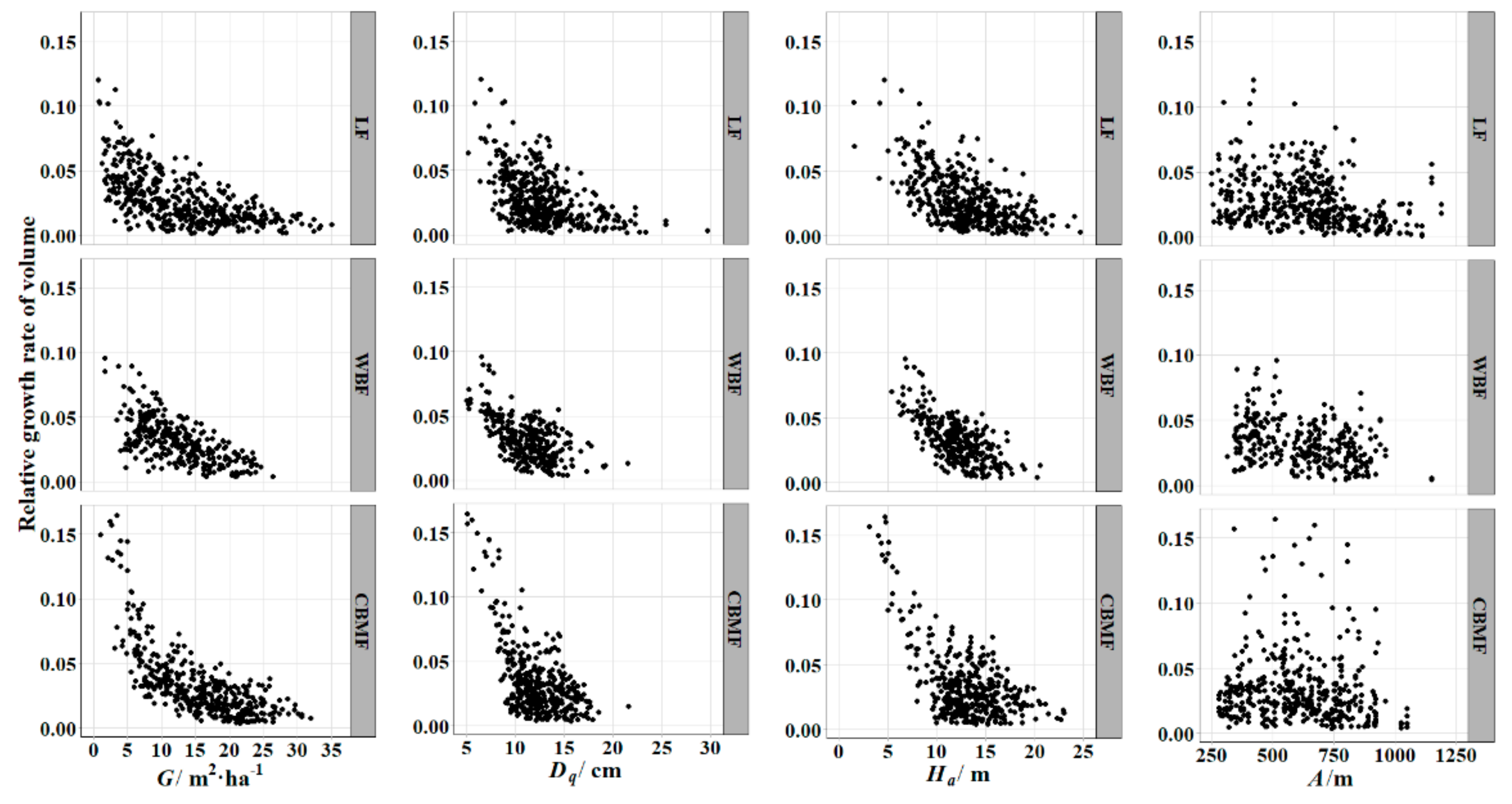
$\alpha$ and $\beta$ are the models’ parameters and X is the independent variable vector. Seven variables were used in the model: (1) altitude ($A$); (2) dominant species mean diameter ($D_d$); (3) quadratic mean diameter of dominant species ($D_q$); (4) stand basal area ($G$); (5) average tree height ($H_a$); (6) the number of trees per hectare ($N$); and (7) slope of the plot ($S$). All models with insignificant variables (p-value > 0.05) were eliminated. The relationship between variables and growth rate are provided in Figure 2. The model fitting performance was evaluated by three evaluation statistics: adjusted coefficient of determination ($R_a{}^2$), root mean square error ($\mathrm{RMSE}$), and Akaike information criterion ($\mathrm{AIC}$). The equation with the largest $R_a{}^2$ and the smallest $\mathrm{RMSE}$ and $\mathrm{AIC}$ was chosen as the best basic model.

$$R_a{}^2=1-\left(\frac{n-1}{n-p}\right)\frac{{{\displaystyle \sum }}_{i=1}^n{\left(y_i-{\widehat{y}}_i\right)}^2}{{{\displaystyle \sum }}_{i=1}^n{\left(y_i-{\stackrel{-}{y}}_i\right)}^2}$$

(9)

$$\mathrm{RMSE}=\sqrt{{\displaystyle \sum }_{i=1}^n{\left(y_i-{\widehat{y}}_i\right)}^2/\left(n-p\right)}$$

(10)

$$\mathrm{AIC}=-2LL+2p$$

(11)

where $n$ is the plots size, $p$ is the number of the model parameters, $LL$ is the log-likelihood value of the equations, and $y_i$, ${\widehat{y}}_i$, and ${\stackrel{-}{y}}_i$ are the observed, predicted, and mean observed volume growth rate, respectively.

Figure 2. Relationship between the $RG{R}_{nv}$ and independent variables for $\mathrm{LF}$, $\mathrm{WBF}$, and $\mathrm{CBMF}$.

The heteroscedasticity is commonly found in growth models. It is well known that the error variance of the $i_{th}$ observation is functionally related to one or more predictors, which can be modeled with a power function, such as ${\sigma }_i^2=(X_i^k$) [33]. The power coefficient k can be obtained by iteratively using the residual variance model $e_i^2=(X_i^k$), in which ${\mathrm{e}}_i$ is the model residual of the unweighted basic model. In this study, we chose $1/{\widehat{y}}_i{}^k$ as the weight function. The Breusch–Pagan test was used to measure the heteroscedasticity corrected model. It uses a variance function and a ${\chi }^2$-test to test the null hypothesis that heteroscedasticity is not present (i.e., homoscedastic) against the alternative hypothesis that heteroscedasticity is present [34]. To ensure that there is no “multicollinearity” in the model, a correlation test method was used.

2.3.2. Nonlinear Mixed-Effects Models

The population average model is commonly used in forestry modeling. However, it cannot exhibit the trends of the specific subjects within the data. A nonlinear mixed-effects model was built to solve this problem, specifically for dealing with the intrinsic variation and the nested structure of the sample data [20,35]. In this study, the best-performing basic model was used to formulate a generalized one-level $\mathrm{NLME}$ growth model by introducing region-level (forest bureau) random effects into the model. All possible combinations of the fixed-effects and random-effects parameters were fitted to the data. The model with the smallest $\mathrm{AIC}$ and the largest log-likelihood ($LL$) was selected for further analyses. A likelihood-ratio test ($\mathrm{LRT}$) was performed to avoid over-parameterization [36]. The one-level NLME growth model can be written as follows:

$${\mathit{y}}_{\mathit{i}}=f\left(\mathit{b},{\mathit{u}}_i,{\mathit{x}}_i\right)+{\mathit{\epsilon }}_i$$

(12)

where ${\mathit{y}}_i={\left[RG{R}_{nv}{}_{i1}, RG{R}_{nv}{}_{i2}, \dots RG{R}_{nv}{}_{i{n}_i}\right]}^T$, ${\mathit{x}}_i={\left[x_{i1}, x_{i2}, \dots x_{i{n}_i}\right]}^T$, and ${\mathit{\epsilon }}_i={\left[{\epsilon }_{i1}, {\epsilon }_{i2}, \dots {\epsilon }_{i{n}_i}\right]}^T$, respectively, represent the vectors of the observation value of $RG{R}_{nv}$, variables, and the random errors; $n_i$ is the number of $RG{R}_{nv}$ measurements for region i; $\mathit{b}$ and ${\mathit{u}}_i$ are vectors of fixed- and random-effects parameters, respectively; ${\mathit{u}}_i$ and ${\mathit{\epsilon }}_i$ are assumed to follow the multivariate normal distributions with mean 0 and variance $D$ and $\mathit{R}$, respectively. $\mathit{D}$ is the variance–covariance matrix of random-effects parameters used in the generalized positive-definite matrix throughout this article, and $\mathit{R}$ is the within-group variance–covariance matrix. The mathematical form is as follows:

$$\mathit{D}=\left[\begin{array}{ccc}{\sigma }_1^2& \cdots & {\sigma }_n{\sigma }_1\\ ⋮& \ddots & ⋮\\ {\sigma }_1{\sigma }_n& \cdots & {\sigma }_n^2\end{array}\right]$$

(13)

$$\mathit{R}={\sigma }^2{\mathit{G}}_i^{0.5}{\mathit{\Gamma }}_i{\mathit{G}}_i^{0.5}$$

(14)

where ${\sigma }_1{}^2$ is the variance of the first parameter; ${\sigma }_n{}^2$ is the variance of the $n$th parameter; ${\sigma }_1{\sigma }_n$ and ${\sigma }_n{\sigma }_1$ are the mutual covariances of the first parameter and the $n$th parameter, respectively; ${\sigma }^2$ is the variance of model residual; ${\mathit{G}}_i$ accounts for within-group variance heteroscedasticity and its diagonal elements are provided by variance function; and ${\mathit{\Gamma }}_i$ accounts for within-group autocorrelations of the residual errors and considered as an identity matrix as there is no time autocorrelation. The heteroscedasticity of the mixed model can be solved by weighted function based on the power variance function, Equation (15).

$$var\left(e_{ij}\right)=\gamma R\widehat{G}{R}_{nv}{}_{ij}^{2\delta }$$

(15)

where $e_{ij}$ and $R\widehat{G}{R}_{nv}{}_{ij}$ are, respectively, the residual and estimated $RG{R}_{nv}$ calculated with fixed-effects for the jth sample plot within the ith sample region, and $\gamma$ and $\delta$ are the estimated parameters for the best basic model. The NLME package in R software was used to obtain the fixed- and random-effects parameters of the nonlinear mixed model of $RG{R}_{nv}$ [37].

To calculate the prediction of $RG{R}_{nv}$ for a new plot, at least one plot of $RG{R}_{nv}$ within each region should be available. The random parameters ${\mathit{u}}_i$ for the plot i can be computed using the first-order of Taylor series expansion [38]:

$${\widehat{\mathit{u}}}_i=\widehat{\mathit{D}}{\mathit{Z}}_i^T{({\mathit{Z}}_i\widehat{\mathit{D}}{\mathit{Z}}_i^T+{\widehat{\mathit{R}}}_i)}^{-1}\left({\mathit{y}}_i-\widehat{\mathit{b}}{\mathit{x}}_i\right)$$

(16)

where ${\widehat{\mathit{u}}}_i$ is the estimate of the random parameters for region i; $\widehat{\mathit{D}}$ is the estimate of D; ${\mathit{Z}}_i$ is the designed matrices for random effects, ${\mathit{Z}}_i$=${\left.\frac{\partial f\left(\mathit{b}, {\mathit{u}}_i,{\mathit{x}}_i\right)}{\partial {\mathit{u}}_i}\right|}_{\widehat{\mathit{b}}, {\widehat{\mathit{u}}}_i}$; ${\mathit{Z}}_i^T$ is the transpose of ${\mathit{Z}}_i$; ${\widehat{\mathit{R}}}_i$ is the estimate of ${\mathit{R}}_i$; ${\mathit{y}}_i$ and ${\mathit{x}}_i$ are the same as defined in Equation (12); and $\widehat{\mathit{b}}$ is estimates of parameter variable. The validation statistic was similar as the basic model, Equations (7)–(9).

2.3.3. Nonlinear Quantile Regressions

The quantile regression model was first introduced by Koenker and Bassett [22] and is also known as a location model. It can characterize the entire conditional distribution of a dependent variable, providing a robust measure of location that reduces the sensitivity of the estimated coefficient to the outlier observations. Quantile regression may bring more efficient estimates than ordinary least-squares regression, specifically when the error term is not normal [39]. $\mathrm{NQR}$ was used to predict $RG{R}_{nv}$ with the $\tau \mathrm{th}$ quantile expressed as:

$${\widehat{\mathit{y}}}_{i\tau }=f\left({\mathit{b}}_{\tau },{\mathit{x}}_i\right)$$

(17)

${\widehat{\mathit{y}}}_{i\tau }=f\left(b_{\tau },x_i\right)$ is the estimated $RG{R}_{nv}$ under the $\tau \mathrm{th}$ quantile, and $\tau$ is the quantile point (ranging from 0 to 1). In contrast to the mean regression technique, which employs the least-squares procedure, the parameters of NQR are obtained by minimizing the following equation [18]:

$$S={\displaystyle \sum }_{y\left(x_{ij}\right)\ge {\widehat{y}}_{\tau }\left(x_{ij}\right)} \tau \left[y\left(x_{ij}\right)-{\widehat{y}}_{\tau }\left(x_{ij}\right)\right]+{\displaystyle \sum }_{y\left(x_{ij}\right)<{\widehat{y}}_{\tau }\left(x_{ij}\right)}\left(1-\tau \right)\left[{\widehat{y}}_{\tau }\left(x_{ij}\right)-y\left(x_{ij}\right)\right]$$

(18)

where $S$ is the sum of the weighted residuals of the $\tau$th quantile; $y\left(x_{ij}\right)$ is the observed $RG{R}_{nv}$. under the ${\tau }_{th}$ quantile; and ${\widehat{y}}_{\tau }\left(x_{ij}\right)$ is the predicted $RG{R}_{nv}$ under the $\tau$th quantile. The quantreg package in R software was used for fitting the $\mathrm{NQR}$ growth rate model [40].

The quantile model can be calibrated with different curves of several quantile points ($\tau$). Three different numbers of quantile points were constructed for the $\mathrm{NQR}$ models—i.e., $\mathrm{NQR}3$ $\left(\tau =0.1, 0.5, 0.9\right)$, $\mathrm{NQR}5$ $\left(\tau =0.1, 0.3, 0.5, 0.7, 0.9\right)$ and $\mathrm{NQR}9$ $(\tau =0.1, 0.2, 0.3, 0.4, 0.5, 0.6, 0.7, 0.8, 0.9$).

When the prior information (a few sampling plot measurements for each region) is utilized in the $RG{R}_{nv}$ $\mathrm{NQR}$ model, the two closest quantile regression curves encompassing the majority of these data points need to be correctly identified [23,41]. One or more $RG{R}_{nv}$ of sample plots were measured in each region as calibration samples to compute the mean difference between the observed and the predicted values of all sample plots for each quantile regression. Two consecutive quantile regressions (i.e., $m$th and$m+1$th) were then chosen for interpolation of the$RG{R}_{nv}$ curve:

$${\widehat{y}}_{ki}=\alpha +\left(1-\alpha \right){\widehat{y}}_{m+1}$$

(19)

where ${\widehat{y}}_i$ is the adjusted quantile regression predicted value of $RG{R}_{nv}$ and the interpolation ratio is $\alpha =\frac{{\widehat{y}}_{m+1}-y_m}{{\widehat{y}}_{m+1}-{\widehat{y}}_m},$ which was obtained by minimization:

$$\mathrm{Q}=\sum \left[(y_{ki}-{\widehat{y}}_{ki}{)}^2\right].$$

(20)

If the mean difference was positive for all the quantile regression curves, then the majority of $RG{R}_{nv}$ were over the highest ($q$th) quantile regression curve, and ${\widehat{y}}_m$ and ${\widehat{y}}_{m+1}$ in Equation (19) were defined as ${\widehat{y}}_{q-1}$ and ${\widehat{y}}_q$, respectively. In contrast, if the mean difference was negative for all quantile regression curves, the ${\widehat{y}}_m$ and ${\widehat{y}}_{m+1}$ were defined as ${\widehat{y}}_1$and ${\widehat{y}}_2$, respectively.

2.3.4. Model Evaluation of Validation and Prediction

Six methods evaluated in this study were: (1) basic model; (2) fixed-effects model; (3) mixed-effects model; (4) $\mathrm{NQR}3$; (5) $\mathrm{NQR}5$; and (6) $\mathrm{NQR}9$. The models were validated using the leave-one-out cross-validation method, which is widely used and considered to be a useful method to test the model’s predictive performance [35]. Three statistics—$MAE$ is mean absolute error, $MPE\left(\%\right)$ is mean percent error, and $MAPE\left(\%\right)$ is mean absolute percent error—were calculated with the model bias generated from validation for assessing and comparing the predictive performance of the models.

$$MAE={\displaystyle \sum }_{i=1}^n\left|\frac{y_i-{\widehat{y}}_i}{n}\right|$$

(21)

$$MPE\left(\%\right)=\frac{{{\displaystyle \sum }}_{i=1}^n\left(y_i-{\widehat{y}}_{i,-i}\right)/y_i}{n}\times 100$$

(22)

$$MAPE\left(\%\right)=\frac{{{\displaystyle \sum }}_{i=1}^n\left|y_i-{\widehat{y}}_{i,-i}\right|/y_i}{n}\times 100$$

(23)

where $y_i$ is the observed $RG{R}_{nv}$, ${\widehat{y}}_{i,-1}$ is the predicted $RG{R}_{nv}$ obtained by the leave-one-out cross-validation method, and $n$ is the size of all plots.

To make more accurate predictions, parameters of the adjusted mixed-effects and quantile regression models should be recalculated and localized using the sampled $RG{R}_{nv}$ in each region and then applied to predict all the other $RG{R}_{nv}$ of plots. One to 15 sample plots were used in this study for each region. Each sample scenario was repeated 500 times to ensure the stability of the results. The evaluation statistics computed for the validation data set are as Equations (21)–(23). We used the paired t-test to compare and analyze the validated results of different sampling numbers and to find the best sample number, considering both accuracy and cost.

Several methods have been suggested for evaluating model predictions, aimed in general at quantifying the relative contribution of different error sources to the unexplained variance [42,43,44]. The most popular method was using graphic plots of observed and predicted data (OP scatter plot). It should be emphasized that the OP scatter plot must set observed values in the y-axis vs. predicted values in the x-axis. The opposite setting will result in incorrect conclusions about the performance of the model. Piñeiro et al. [45] suggested that the coefficient of determination of the regression of OP values ($R^2$) is an effective parameter that provides important information about model performance to indicate how much of the linear variation of observed values is explained by the variation of predicted values. It was calculated by Equation (24), where $y_i$ was the observed $RG{R}_{nv}$ and $\widehat{{\widehat{y}}_i}$ was the predicted $RG{R}_{nv}$. Another suggestion was to test the hypothesis of slope = 1 and intercept = 0 to assess statistically the significance of regression parameters of fitting relationship between the observed and predicted data.

$$R^2=1-\frac{{{\displaystyle \sum }}_{i=1}^n{\left(y_i-\widehat{{\widehat{y}}_i}\right)}^2}{{{\displaystyle \sum }}_{i=1}^n{\left(y_i-{\stackrel{-}{y}}_i\right)}^2}.$$

(24)

3. Results

3.1. Best Basic Model

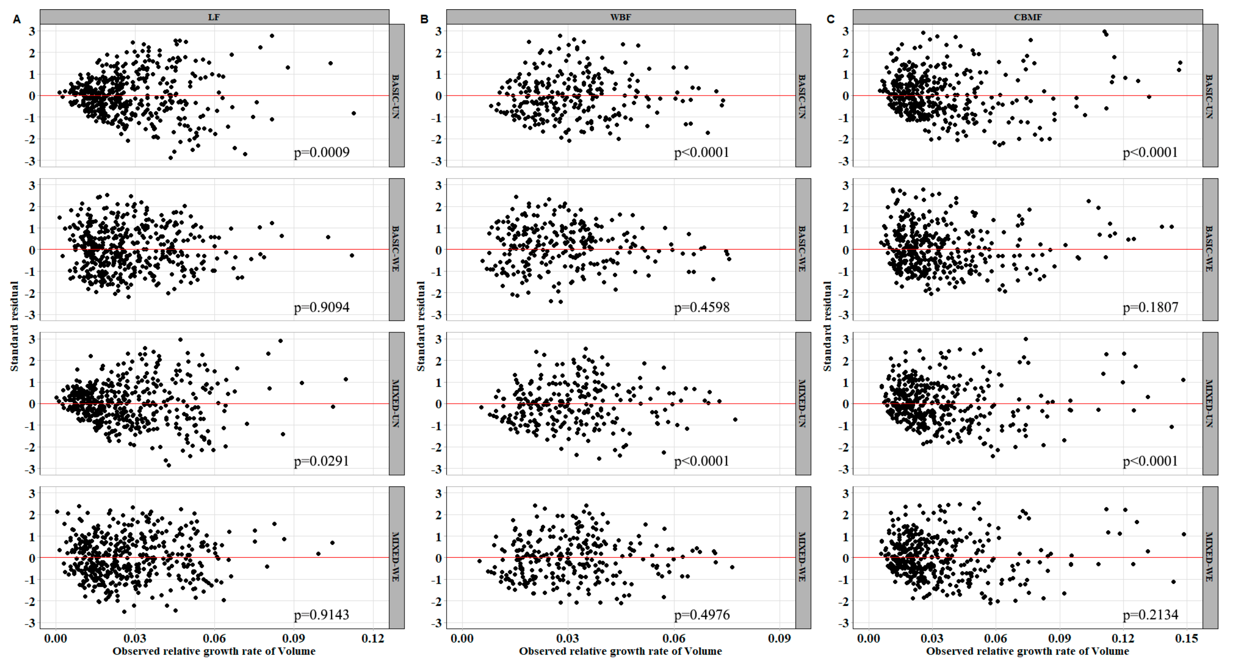
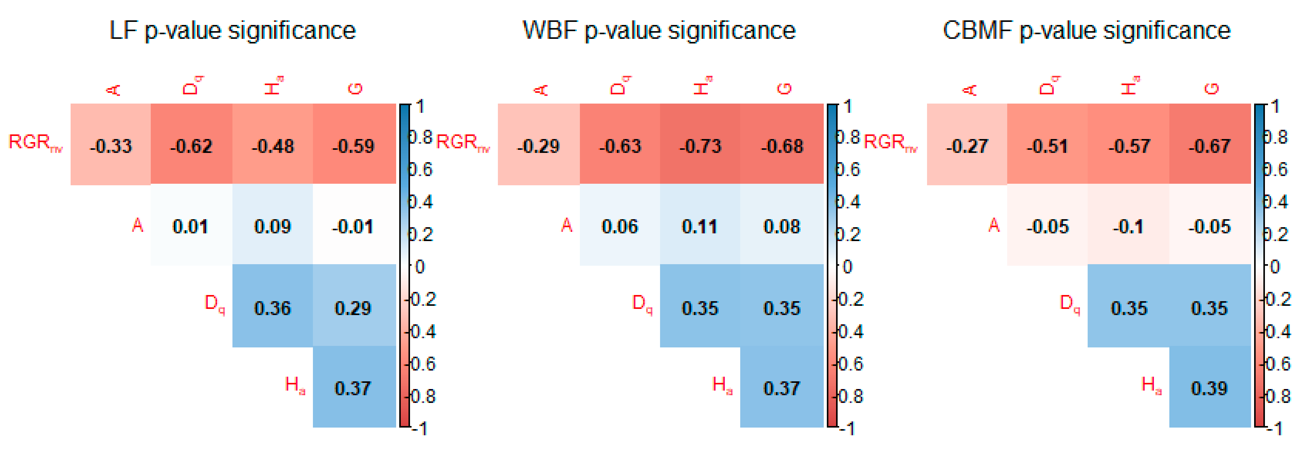
The fitting results of the basic models are provided in the Appendix A (Table A1, Table A2 and Table A3). The best basic $RG{R}_{nv}$ model form was the exponential function model for all the three forest types. The $R_a{}^2$ and $\mathrm{RMSE}$ for the best basic model is 0.6841 and 0.0111 ($\mathrm{LF}$), 0.6991 and 0.0087 ($\mathrm{WBF}$), and 0.8031 and 0.0122 ($\mathrm{CBMF}$), respectively (Table 3). The parameter estimates and standard errors are shown in the Appendix A (Table A4, Table A5 and Table A6). The relationship between the variables and the $RG{R}_{nv}$ is presented in Figure 2. The heteroscedasticity of the model significantly stabilized (p > 0.05) after the model was weighted (Figure 3). The variables correlation test (Figure 4) showed that there was no obvious strong correlation (−0.6 < coefficient values < 0.6) between the model independent variables [46]. The specific form of the model is as follows:

$$RG{R}_{nv}=a_1\exp \left({\beta }_1{D}_q+{\beta }_{2}G+{\beta }_3{H}_a+{\beta }_{4}A\right)$$

(25)

Table 3. Model fitting of the best basic and mixed-effects model for the three forest types.

Forest Types	Model	Fitting Statistics
		${\mathit{R}}_{\mathit{a}}^2$	$\mathbf{R}\mathbf{M}\mathbf{S}\mathbf{E}$	$\mathbf{A}\mathbf{I}\mathbf{C}$
LF	Basic	0.6841	0.0111	−2781.33
	Mixed	0.7706	0.0095	−2930.69
WBF	Basic	0.6990	0.0086	−1760.76
	Mixed	0.7978	0.0071	−1862.14
CBMF	Basic	0.8031	0.0122	−2372.05
	Mixed	0.8546	0.0104	−2474.67

Figure 3. Standardized residual plots for the basic and mixed-effects models of the three forest types ((A): LF, (B): WBF and (C): CBMF); BASIC-UN, BASIC-WE, MIXED-UN, and MIXED-WE represent the unweighted basic model, the weighted basic model, the unweighted mixed-effects model, and the weighted mixed-effects model, respectively.

Figure 4. Variables correlation test diagram of the three forest types.

3.2. Mixed-Effects Models

The parameter estimations of the mixed-effects models are presented in the Appendix A (Table A4, Table A5 and Table A6). Different random parameter combinations were sequentially added to the basic model. The best mixed-effects models for the three forest types were finally determined after considering the model convergence and the comparison of fitting indicators. The model forms for LF, WBF and CBMF are as follows ($u_1$–$u_4$ are random parameters):

$$RG{R}_{nv}=a_1\exp (\left({\beta }_1+u_1\right)D_q+{\beta }_{2}G+{\beta }_3{H}_a+({\beta }_4+u_4)\mathrm{A})$$

(26)

$$RG{R}_{nv}=a_1\exp \left({\beta }_1{D}_q+({\beta }_2+u_2\right)G+({\beta }_3+u_3)H_a+{\beta }_4\mathrm{A})$$

(27)

$$RG{R}_{nv}=a_1\exp \left({\beta }_1{D}_q+({\beta }_2+u_2\right)G+({\beta }_3+u_3)H_a+{\beta }_4\mathrm{A})$$

(28)

The model fitting accuracy significantly improved after the addition of random effects to the basic model, in which their $R_a{}^2$ and $\mathrm{RMSE}$ were 0.7706 and 0.0095 ($\mathrm{LF}$), 0.7978 and 0.0071 ($\mathrm{WBF}$), and 0.8546 and 0.0104 ($\mathrm{CBMF}$), respectively (Table 3). As in the previous subsection, the heteroscedasticity of the mixed-effects models also significantly stabilized (p > 0.05) after it was weighted (Figure 3).

3.3. Nonlinear Quantile Regression Models

The parameter estimates and standard errors of the $\mathrm{NQR}$ models across different quantile points are shown in Appendix A (Table A4, Table A5 and Table A6). Quantile regression properly represented the characteristics of invariant to monotonic transformations; hence, the heteroscedasticity or outliers had only an insignificantly minor effect on the $\mathrm{NQR}$ estimations. Table 4 shows no difference in $\mathrm{MAE}$ values between $\mathrm{NQR}3$, $\mathrm{NQR}5$, and $\mathrm{NQR}9$. $\mathrm{NQR}9$ had smaller $\mathrm{MPE}\left(\%\right)$ and $\mathrm{MAPE}\left(\%\right)$ than $\mathrm{NQR}3$ and $\mathrm{NQR}5$, indicating that it provided slightly better predictions than the other two methods.

Table 4. Model validation statistics of the six different methods for $\mathrm{LF}$, $\mathrm{WBF}$, and $\mathrm{CBMF}$.

Forest Types	Model	Validation for Model Statistics
		$\mathbf{M}\mathbf{A}\mathbf{E}$	$\mathbf{M}\mathbf{P}\mathbf{E}\left(\mathit{\%}\right)$	$\mathbf{M}\mathbf{A}\mathbf{P}\mathbf{E}\left(\mathit{\%}\right)$
LF	Basic	0.0091	−33.0941	56.7638
	Fixed	0.0094	−36.9125	59.9228
	Mixed	0.0079	−27.3283	46.0380
	NQR3	0.0078	−19.9447	43.4524
	NQR5	0.0078	−18.0479	42.3543
	NQR9	0.0078	−15.4803	41.5027
WBF	Basic	0.0073	−15.3719	33.8379
	Fixed	0.0081	−16.0116	33.9058
	Mixed	0.0058	−11.8536	26.7588
	NQR3	0.0058	−9.3290	24.8674
	NQR5	0.0058	−9.5704	24.9588
	NQR9	0.0058	−9.3227	24.5826
CBMF	Basic	0.0094	−16.0511	41.4629
	Fixed	0.0099	−17.0285	41.8236
	Mixed	0.0088	−16.5065	38.2697
	NQR3	0.0087	−12.5448	36.1170
	NQR5	0.0087	−11.8615	36.1139
	NQR9	0.0085	−10.7174	34.0156

3.4. Comparison of $RG{R}_{nv}$ between Three Forest Types

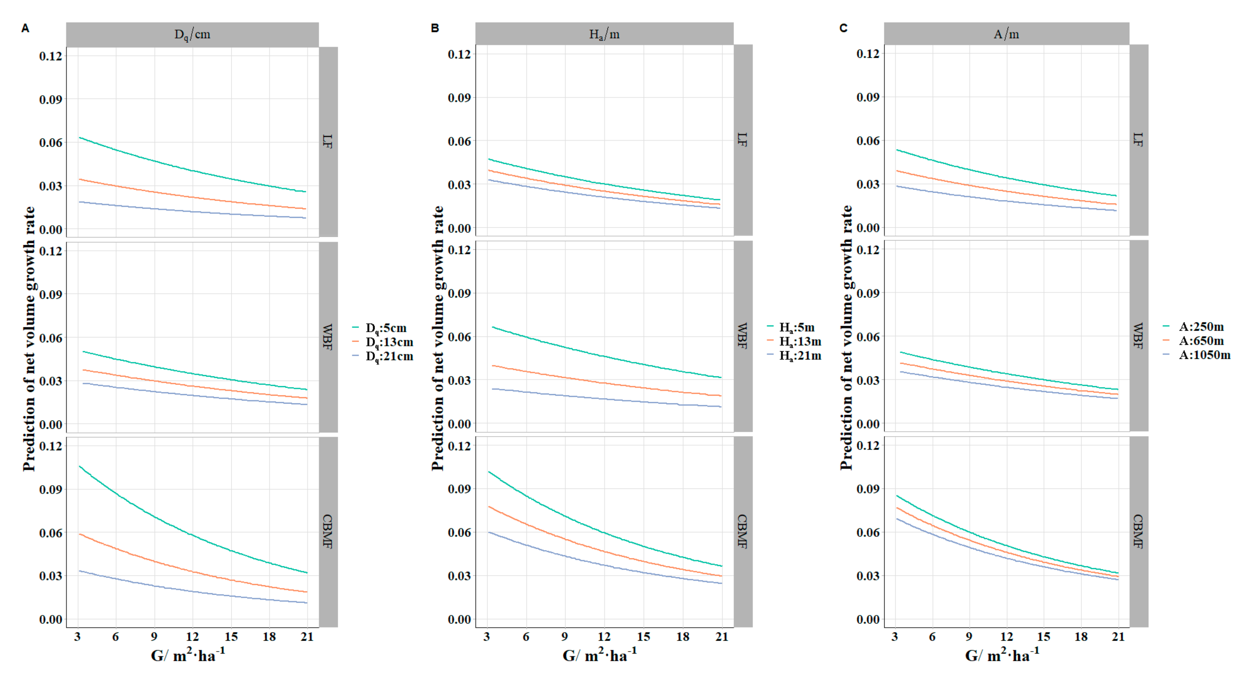
Four variables were included in the basic model (Equation (25)), which were $D_q$, $G$, $H_a$, and $A$. To compare $RG{R}_{nv}$ between the three forest types, the relationship between the predicted $RG{R}_{nv}$ and $G$ at different variable levels was visualized, since $G$ had a superior performance in the basic model compared to the other variables. The common data interval range of the remaining variables in each stand was determined according to the maximum and minimum value, then the average value was calculated and divided into three levels. The results are shown in Figure 5.

Figure 5. The relationship between $RG{R}_{nv}$ and $G$ at three different levels of $D_q$ (A), $H_a$ (B), and $A$ (C); the mean values of $D_q$, $H_a$, and $A$ are 11.1 cm, 12.2 m, and 625.9 m for $\mathrm{LF}$; 12.8 cm, 13.1 m, and 635.3 m for $\mathrm{WBF}$; and 12.2 cm, 13.1 m, and 601.9 m for $\mathrm{CBMF}$.

For $\mathrm{LF}$, the $RG{R}_{nv}$ across three levels of $D_q$ differed more than $H_a$ and $A$. This result indicated that the effect of the individual’s radial size on the growth rate was higher than that of the longitudinal size and site in LF. The opposite result was found in $\mathrm{WBF}$, where the $RG{R}_{nv}$ differences among the average $H_a$ values were greater than other variables. For $\mathrm{CBMF}$, the differences among both $D_q$ and $H_a$ were greater than $A$. The $RG{R}_{nv}$ rank among the three stand types varied across diameter levels (Figure 5A), when the $D_q$ were 5 and 13 cm, the $RG{R}_{nv}$ was ranked as $\mathrm{CBMF}$ > $\mathrm{LF}$ > $\mathrm{WBF}$. The order changed when $D_q$ was 21 cm: $\mathrm{WBF}$ > $\mathrm{CBMF}$ > $\mathrm{LF}$. For both $H_a$ and $A$, $\mathrm{CBMF}$ consistently had the highest $RG{R}_{nv}$ across all the three levels.

3.5. Comparing Modeling Approaches

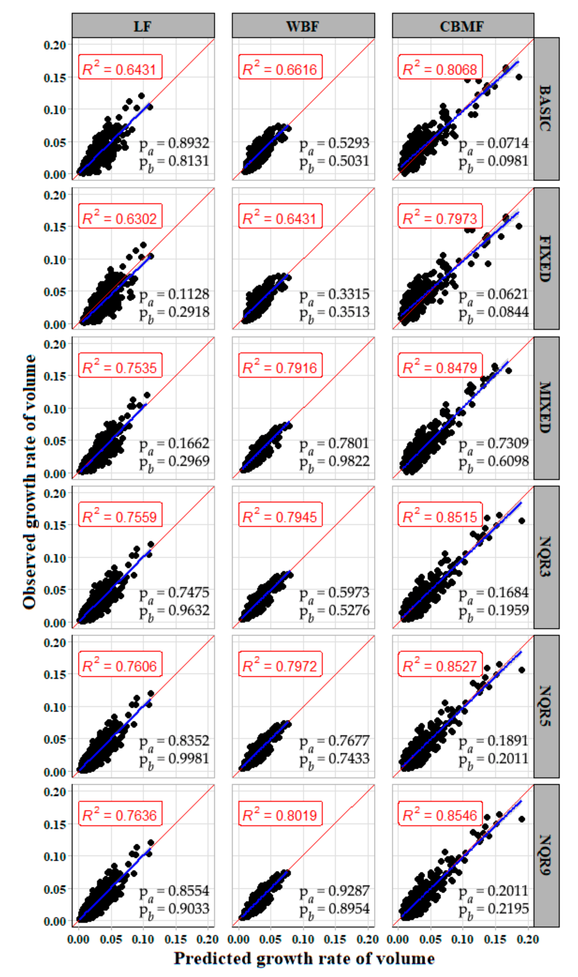
Table 4 presents the model validation results using the leave-one-out validation method. The results showed that the basic model provided a slightly higher accuracy than the fixed-effects model. In addition, the $\mathrm{MPE}\left(\%\right)$ and$\mathrm{MAPE}\left(\%\right)$ values of the mixed-effects and quantile model were significantly lower compared to the basic model, in which the quantile model resulted a way much better prediction than the mixed-effects model. For the quantile model, $\mathrm{NQR}9$ was better than $\mathrm{NQR}5$ and $\mathrm{NQR}3$ in both $\mathrm{LF}$ and $\mathrm{CBMF}$. There was only a slight prediction difference between the $\mathrm{NQR}3$, $\mathrm{NQR}5$, and $\mathrm{NQR}9$ in $\mathrm{WBF}$. Figure 6 shows the scatter plots between the observed and predicted $RG{R}_{nv}$ of the basic, fixed-effects, mixed-effects, and quantile models. $\mathrm{NQR}9$ had the biggest ${\mathrm{R}}^2,$ indicating that it performed best among all the methods. Both null hypotheses were not rejected; thus, disagreement between model predictions and observed data was due entirely to the unexplained variance.

Figure 6. Plot for the observed and predicted $RG{R}_{nv}$ of the $\mathrm{BASIC}$, $\mathrm{FIXED}$, $\mathrm{MIXED}$, $\mathrm{NQR}3$, $\mathrm{NQR}5$, and $\mathrm{NQR}9$ models.

3.6. Comparison of Sample Size for Calibration

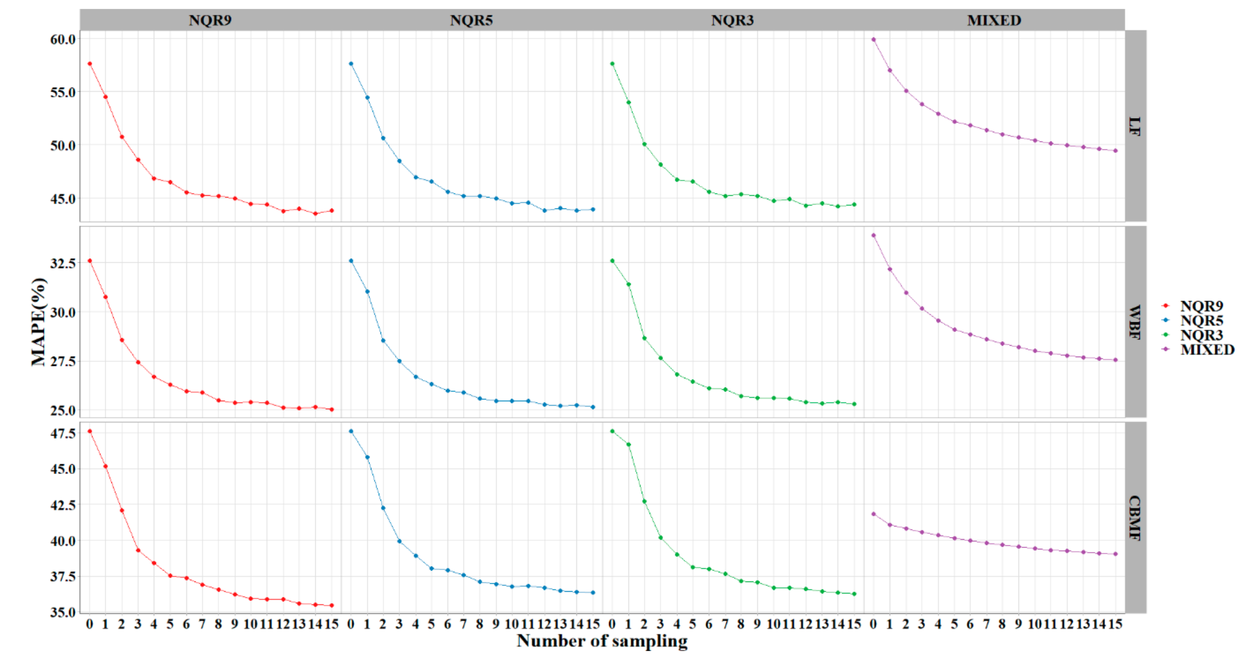
Figure 7 presents the $\mathrm{MAPE}\left(\%\right)$ variation across various sample numbers for the four models ($\mathrm{NQR}9$, $\mathrm{NQR}5$, $\mathrm{NQR}3$, and the mixed-effects model). Zero sample number means that $\mathrm{MAPE}\left(\%\right)$ was calculated using the mixed-effects model with fixed parameters only, and for the quantile regression, $\mathsf{\tau }=0.5$ refers to the median effect. The $\mathrm{MAPE}\left(\%\right)$ values decreased as the sample numbers increased across all forest types, in which the three quantile regressions (i.e., $\mathrm{NQR}3$, $\mathrm{NQR}5$, and $\mathrm{NQR}9$) had lower $\mathrm{MAPE}\left(\%\right)$ values than the mixed-effects model. The difference between $\mathrm{NQR}9$, $\mathrm{NQR}5$, and $\mathrm{NQR}3$ was not obvious, where $\mathrm{NQR}9$ consistently outperformed $\mathrm{NQR}3$ and $\mathrm{NQR}5$ by producing the lowest $\mathrm{MAPE}\left(\%\right)$ values across all sample numbers. The above conclusion was confirmed statistically by a series of test of contrasts: sample of one plot per region vs. two or more plots; two plots vs. three or more plots, etc. Results indicated that sampling six plots per region yielded non-significant differences among the evaluation statistics as compared to sampling seven or more plots (Table 5). Hence, more stable $\mathrm{MAPE}\left(\%\right)$ performances were seen when the sample numbers were greater than or equal to six.

Figure 7. The relationship between $\mathrm{MAPE}\left(\%\right)$ and sampling numbers (plots/region) across the four models and three forest types.

Table 5. Testing of contrasts of sample plots with the result of NQR9 for LF, WBF, and CBMF. A bold, underlined number denotes a significant difference (p < 0.05) in the test of contrasts.

Contrasts	p-Level
	LF	WBF	CBMF
1 plot vs. 2 and more plots	<0.0001	<0.0001	<0.0001
2 plot vs. 3 and more plots	<0.0001	<0.0001	<0.0001
3 plot vs. 4 and more plots	<0.0001	<0.0001	<0.0001
4 plot vs. 5 and more plots	0.0013	0.0023	0.0006
5 plot vs. 6 and more plots	0.0135	0.0089	0.0013
6 plot vs. 7 and more plots	0.1887	0.3057	0.0841
7 plot vs. 8 and more plots	0.1919	0.3223	0.1261
8 plot vs. 9 and more plots	0.2952	0.3554	0.2578
9 plot vs. 10 and more plots	0.3524	0.4666	0.388
10 plot vs. 11 and more plots	0.5746	0.4981	0.4548
11 plot vs. 12 and more plots	0.6406	0.5721	0.5855
12 plot vs. 13 and more plots	0.7813	0.7841	0.6901
13 plot vs. 14 and more plots	0.8862	0.8491	0.7067
14 plot vs. 15 and more plots	0.9321	0.8843	0.7498

For the mixed-effects models, the result of sampling indicated that when the sample size was more than six (Appendix A: Table A7), the following occurred: (1) $\mathrm{MAE}$ decreased by about 9.9%, 25.1%, and 2.1% for LF, WBF, and CBMF, respectively; (2) $\mathrm{MPE}\left(\%\right)$ decreased by about 15.6%, 17.3%, and 6.3% for LF, WBF, and CBMF, respectively; (3) $\mathrm{MAPE}\left(\%\right)$ decreased by about 14.2%, 15.6%, and 4.8% for LF, WBF, and CBMF, respectively. The results were varied across the three forest types for the three quantile regression models, in which: (1) the $\mathrm{MAE}$ of the $\mathrm{NQR}3$,$\mathrm{NQR}5$, and $\mathrm{NQR}9$ decreased by about 24.7%, 25.3%, and 25.6% for $\mathrm{LF}$; 26.2%, 26.3%, and 26.5% for $\mathrm{WBF}$; and 24.2%, 24.7%, and 24.8% for $\mathrm{CBMF}$, respectively; (2) the $\mathrm{MPE}\left(\%\right)$ of the $\mathrm{NQR}3$,$\mathrm{NQR}5$, and $\mathrm{NQR}9$ decreased by about 27.5%, 28.0%, and 30.0% for $\mathrm{LF}$; 10.2%, 13.1%, and 15.3% for $\mathrm{WBF}$; and 34.9%, 37.5%, and 40.2% for $\mathrm{CBMF}$, respectively; (3) the $\mathrm{MAPE}\left(\%\right)$ of the $\mathrm{NQR}3$,$\mathrm{NQR}5$, and $\mathrm{NQR}9$ decreased by about 21.2%, 21.3%, and 21.3% for $\mathrm{LF}$; 20.4%, 20.8%, and 20.9% for $\mathrm{WBF}$; and 21.0%, 21.2%, and 22.4% for $\mathrm{CBMF}, \mathrm{respectively}$.

4. Discussion

In this study, Equation (25) was the best basic $RG{R}_{nv}$model constructed using four primary predictors: $D_q$, $G$, $H_a$, and $A$. The data were obtained from the $\mathrm{NFI}$’s permanent sample plots across the three forest types in eastern Daxing’an Mountains. The exponential form was found to be the best basic $RG{R}_{nv}$model. Several previous studies have proven that the exponential form can visualize the important biological characteristics of various animal and plant growth. Jobidon [47] studied the competition effects in the boreal mixed wood forest across Quebec and Canada; he concluded that the exponential form should be considered to analyze the stand growth, specifically if young trees exist. Scolforo et al. [48] also preferred to utilize the exponential form to model the relative diameter growth rate of the six tree species in Brazil, which included stand density as the primary predictors. The exponential model was proposed in this study since it was able to clearly describe the growth rate of the cold temperate forests and avoid negative growth rate estimation. Most of the native tree species had small $\mathrm{DBH}$, while only a few individual trees had large $\mathrm{DBH}$. Hence, these larger trees have smaller predicted growth rate values compared to other trees. The larger trees may highly influence the model; however, the exponential formulation does not allow the predicted growth rate to be negative.

The $RG{R}_{nv}$ was the dependent variable of the model in this paper and was calculated with Pressler’s formula using the average growth rate to replace the consecutive annual growth rate. $RG{R}_{nv}$ is a standard variable to determine the productive capacity of a tree and can be used to compare the trees that differ in initial size, age, and environmental conditions [49,50]. All four parameter estimates were negative, indicating that the $RG{R}_{nv}$ decreased with the increment of various variables. This trend was consistent with the actual survey results (Figure 2).

$D_q$ was used for the average tree diameter in the research of tree growth, having a better performance than the arithmetic mean diameter [51,52]. Curtis et al. [53] explained the difference between the average and the arithmetic mean diameter in detail and their respective applicable scenarios. Reineke’s [54] $\mathrm{SDI}$ (stand density index) was used for the various relative density measures and stand management diagrams derived from the Reineke relationship, which was based on $D_q$. $H_a$ was also an important variable for describing stand structure, specifically for the vertical direction. $G$ was the density index, combining the tree diameter and the number of trees within a stand. Site effect variables that contained altitude, slope, and aspect have been recommended in growth, forest species composition, and productivity research [55,56,57]. Unfortunately, in this study, although the altitude showed significant contributions to the $RG{R}_{nv}$ model, the slope and aspect of the plot were not significant in the model. The $RG{R}_{nv}$ declined with altitude, which could be the result of a short growing season and reduction in mean summer temperatures [58,59]. Ma and Lei [60] showed that $H_a$ can replace dominant height when there is no information available. However, Inoue [61] found that stand volume and bole surface area were not independent of stand age or site quality. Hence, when the stand age is unknown, $H_a$ can be the average feedback of stand vertical structure rather than the stand site condition.

The growth of the trees has played an important role in recycling the forest. Plantation forests emerged mainly in Germany and Austria, while the concept of natural forests originated in France and Switzerland [62]. Although some research on heterogeneous forests was conducted in 1940s, presently, natural forests are still lacking a forest management philosophy. Dahurian larch is a very intolerant and cold-resistant species that can grow in dry, infertile, and swamped soil, or on permanently frozen ground; however, it is best grown in drained, moist, and sandy soil [63]. Jia and Zhou [64] summarized the growth characteristics of natural and planted Dahurian larch in Northeast China. They emphasized that the growth rates are considered essential indexes in assessing forest recovery processes and carbon sequestration potentials, which can supply post-fire or sustainable management strategies. White birch is an excellent, fast-growing pioneer species and suitable for well-drained soil; it can grow in heavy clay and nutritionally poor soils [65]. In recent years, research on the mixed forest has developed rapidly, including stand stability [66], stand resource utilization [67], stand diversity [68], and stand dynamic change [69]. It has shown that the mixed forest has obvious advantages over the pure forest. The $\mathrm{CBMF}$ studied in this paper mainly involved the mixed forest of $\mathrm{LF}$ and $\mathrm{WBF}$. Figure 5 shows that the $RG{R}_{nv}$ of $\mathrm{CBMF}$ was higher than $\mathrm{LF}$ and $\mathrm{WBF}$ across different levels, which proved that $\mathrm{CBMF}$ had more potential growth superiority compared with $\mathrm{LF}$ and $\mathrm{WBF}$. $\mathrm{CBMF}$ also has the highest productivity or stand stability, which was corroborated by the well-known competitive yield criterion [70].

In forestry applications, two or more measurements are often taken from each sampling unit. These repeated measurements are not statistically independent; hence, the ordinary least-squares techniques may underestimate the variance of parameters. In this paper, the nonlinear mixed model and quantile model were used to deal with the longitudinal data. According to Table 3, the prediction accuracy of all $\mathrm{NLME}$ models was improved and presented a more stable estimate (indicating the reduction of spatial heterogeneity in the model residuals). $\mathrm{WBF}$ had the most significant improvement, which was then followed by $\mathrm{LF}$ and $\mathrm{CBMF}$. Figure 6 shows that the relationship between the observed value and the predicted value of the mixed model was more concentrated compared with the basic model. The random effect was integrated to $D_q$ and $\mathrm{A}$ for the $\mathrm{LF}$ mixed model, while $G$ and $H_a$ were used for $\mathrm{WBF}$ and $\mathrm{CBMF}$, corroborating the results of Condés and García-Robredo [71]. Zhao et al. [72] reported that modeling the autocorrelation structure alone cannot completely match the possible common effects, and they suggested introducing random period effects for describing the autocorrelation. Unfortunately, their research relied only on one to three observations; hence, it is unreliable to employ period as an autocorrelation structure.

Cade and Noon [73] mentioned that the quantile regression estimates multiple rates of change (slopes) from the minimum to maximum response, providing a more complete trend of the variables relationships. Table 4 shows that the result of the quantile regression model was better than the basic and $\mathrm{NLME}$ models. $\mathrm{MPE}\left(\%\right)$ and $\mathrm{MAPE}\left(\%\right)$ indicated that more improvement in model accuracy existed for the quantile regression than for the $\mathrm{NLME}$ models.$\mathrm{NQR}9$ was a better quantile regression than the others ($\mathrm{NQR}3$ and $\mathrm{NQR}5$), although the difference was negligible. Bohora and Cao [26] showed that $\mathrm{NQR}3$ was better than $\mathrm{NQR}5$ and $\mathrm{NQR}9$, while Zang et al. [24] argued that $\mathrm{NQR}9$ was the best and used it to model the height–diameter relationship. This kind of contradictory result may be caused by the size and the distribution of the data. The higher quantiles require a much greater proportional increase in data volume to maintain a constant risk ratio, and the excessive numbers of the quantile may cause over-fitting. Therefore, we recommend choosing $\mathrm{NQR}3$ or $\mathrm{NQR}5$ when the data distribution range is narrow or when the size of the data is limited. In this study, the quantile model had a better result than the $\mathrm{NLME}$, which was indicated by smaller $\mathrm{MAE}$, $\mathrm{MPE}\left(\%\right)$, and $\mathrm{MAPE}\left(\%\right)$. The reason might be the obvious differences in growth rate trends between different regions.

Random sampling was used to calibrate the mixed-effects and quantile models. The results showed that the model performance improved with an increase in the sampling number. The quantile model performed better than the mixed model across all sample numbers, and NQR9 was best among them. Six (or more) sample plots per region were adequate for delivering high-accuracy predictions (Figure 7, Table 5). In the mixed-effects or the quantile regression model, the subject-specific random effect or entire conditional distribution of the response makes up the shortcomings of instability and uncertainty of the population-averaged response. The sampling process is a hypothetical simulation of the survey in reality. It can provide prior information to adjust the random parameters or interpolation ratio of the local best quantile curve and effectively improve the accuracy of estimation. It has generally been taken for granted that the inclusion of additional stand variables into the base models automatically results in better predictions (helping to justify the increased costs associated with measuring the additional variables). As Huang et al. [74] stated, the subject-specific model allows the plot level variations related to many known and unknown factors such as topography, soil type, nutrient status, genetics, climate, silvicultural regime, environment, intra- and inter-specific competitions, etc., to be accounted for without requiring that they be identified or measured. This is a noted advantage of the $\mathrm{NLME}$ and $\mathrm{NQR}$ techniques. In this study, each region contained an average of 32 plots. Assuming the data from the last period are known, the next period $RG{R}_{nv}$ of all plots can be estimated when only six plots from each region are surveyed. This can save about 80% of costs.

5. Conclusions

Plantation forests have developed rapidly in modern forestry because of their simple structure, short management cycle, and high timber output. However, there is still a lack of a theoretical basis for natural pure forests and mixed forests. Hence, in this study three forest types from Daxing’an Mountains were studied to determine the growth differences between the natural pure forest and mixed forest and establish the $RG{R}_{nv}$ model. $RG{R}_{nv}$ was recalculated with the Pressler growth rate formula. The liner model, reciprocal model, power model, exponential model, and sigmoid model were used to develop the basic model, and of these, the exponential model performed the best. The best $RG{R}_{nv}$ basic model was established using $D_q$, $G$, $H_a$, and $A$ surveyed from three periods, using $\mathrm{NFI}$ data from 12 forest bureaus in the eastern Daxing’an Mountains, Northeast China, for a total of 1152 samples. A correlation index plot showed that there was no obvious strong relationship between the independent variables. The exponential model was proposed in this study since it was able to clearly describe the growth rate of the cold temperate forests and avoid negative growth rate estimation. All four parameter estimates were negative, indicating that $RG{R}_{nv}$ decreased with an increment in various variables. This trend was consistent with the actual survey results. The result showed that the trend of $RG{R}_{nv}$ differed among the three forest types, in which $\mathrm{CBMF}$ had higher $RG{R}_{nv}$ than both $\mathrm{LF}$ and $\mathrm{WBF}$, indicating the superiority of mixed forest.

In this paper, four different methods, i.e., $\mathrm{NLME}$, $\mathrm{NQR}3$, $\mathrm{NQR}5$, and $\mathrm{NQR}9,$ were used to deal with the longitudinal data. All models were validated using the leave-one-out method and random sampling technique. Both quantile regression and $\mathrm{NLME}$ methods showed better performance than the basic model. After the addition of random effects, the $R_a^2$ improved: 0.6841 to 0.7706 ($\mathrm{LF}$), 0.6990 to 0.7978 ($\mathrm{WBF}$), and 0.8031 to 0.8546 ($\mathrm{CBMF}$). $\mathrm{NQR}9$ outperformed all methods evaluated in this study and provided the best $\mathrm{MAE}$, $\mathrm{MPE}\left(\%\right)$, and $\mathrm{MAPE}\left(\%\right)$ values. Model weighting effectively removed the heteroscedasticity effect of the basic and mixed models. Performance of the methods improved as the sample size increased. Six (or more) sample plots was the most appropriate number and is recommended for model calibration when both prediction accuracy and sampling cost are considered.

References

1. FAO. Global Forest Resources Assessment. In Main Report; FAO: Rome, Italy, 2020. [Google Scholar]
2. National Forestry and Grassland Administration (NFGA). China Forest Resources Report: 2014–2018; China Forestry Publishing House: Beijing, China, 2019; p. 108. (In Chinese) [Google Scholar]
3. Pommerening, A.; Muszta, A. Methods of modelling relative growth rate. For. Ecosyst. 2015, 2, 5. [Google Scholar] [CrossRef] [Green Version]
4. Jørgensen, S.E.; Patten, B.C.; Straškraba, M. Ecosystems emerging: Toward an ecology of complex systems in a complex future. Ecol. Model. 1992, 62, 1–27. [Google Scholar] [CrossRef]
5. Ritchie, M.W.; Hann, D.W. Implications of disaggregation in forest growth and yield modeling. For. Sci. 1997, 43, 223–233. [Google Scholar]
6. Soares, P.; Tomé, M.; Skovsgaard, J.P.; Vanclay, J.K. Evaluating a growth model for forest management using continuous forest inventory data. For. Ecol. Manag. 1995, 71, 251–265. [Google Scholar] [CrossRef]
7. Hunt, R. Plant Growth Curves. In The Functional Approach to Plant Growth Analysis; Cambridge University Press: Cambridge, UK, 1982; p. 248. [Google Scholar]
8. Zeide, B. Analysis of Growth Equations. For. Sci. 1993, 39, 594–616. [Google Scholar] [CrossRef]
9. Zhang, L.J. Cross-validation of Non-linear Growth Functions for Modelling Tree Height–Diameter Relationships. Ann. Bot. 1997, 79, 251–257. [Google Scholar] [CrossRef] [Green Version]
10. Vanclay, J.k. Modelling Forest Growth and Yield: Applications to Mixed Tropical Forests; CAB International: Wallingford, UK, 1994. [Google Scholar]
11. Moser, J.W.; Hall, O.F. Deriving growth and yield functions for uneven-aged forest stands. For. Sci. 1969, 15, 183–188. [Google Scholar]
12. Dale, V.H.; Doyle, T.W.; Shugart, H.H. A comparison of tree growth models. Ecol. Model. 1985, 29, 145–169. [Google Scholar] [CrossRef]
13. Peng, C. Growth and yield models for uneven-aged stands: Past, present and future. For. Ecol. Manag. 2000, 132, 259–279. [Google Scholar] [CrossRef]
14. Laubhann, D.; Sterba, H.; Reinds, G.J.; De Vries, W. The impact of atmospheric deposition and climate on forest growth in European monitoring plots: An individual tree growth model. For. Ecol. Manag. 2009, 258, 1751–1761. [Google Scholar] [CrossRef]
15. Causton, D.R.; Venus, J.C. The Biometry of Plant Growth; Edward Arnold: London, UK, 1981; p. 17. [Google Scholar]
16. Muller, H.-G.; Stadtmuller, U. Estimation of Heteroscedasticity in Regression Analysis. Ann. Stat. 1987, 15, 610–625. [Google Scholar] [CrossRef]
17. Dong, L.; Zhang, L.; Li, F.R. Additive Biomass Equations Based on Different Dendrometric Variables for Two Dominant Species (Larix gmelini Rupr. and Betula platyphylla Suk.) in Natural Forests in the Eastern Daxing’an Mountains, Northeast China. Forests 2018, 9, 261. [Google Scholar] [CrossRef] [Green Version]
18. Zhang, X.-Q.; Lei, Y.-C.; Liu, X.-Z. Modeling stand mortality using Poisson mixture models with mixed-effects. iForests 2015, 8, 333–338. [Google Scholar] [CrossRef]
19. Timilsina, N.; Staudhammer, C.L. Individual Tree-Based Diameter Growth Model of Slash Pine in Florida Using Nonlinear Mixed Modeling. For. Sci. 2013, 59, 27–37. [Google Scholar] [CrossRef]
20. Fu, L.; Zhang, H.; Sharma, R.P.; Pang, L.; Wang, G. A generalized nonlinear mixed-effects height to crown base model for Mongolian oak in northeast China. For. Ecol. Manag. 2017, 384, 34–43. [Google Scholar] [CrossRef]
21. Sharma, R.P.; Breidenbach, J. Modeling height-diameter relationships for Norway spruce, Scots pine, and downy birch using Norwegian national forest inventory data. For. Sci. Technol. 2014, 11, 44–53. [Google Scholar] [CrossRef]
22. Koenker, R.; Bassett, G.J. Regression quantiles. Econometrica 1978, 46, 33–50. [Google Scholar] [CrossRef]
23. Cao, Q.V.; Wang, J. Evaluation of Methods for Calibrating a Tree Taper Equation. For. Sci. 2015, 61, 213–219. [Google Scholar] [CrossRef] [Green Version]
24. Zang, H.; Lei, X.; Zeng, W. Height-diameter equations for larch plantations in northern and northeastern China: A comparison of the mixed-effects, quantile regression and generalized additive models. For. Int. J. For. Res. 2016, 89, 434–445. [Google Scholar] [CrossRef]
25. Galarza, C.E.; Castro, L.M.; Louzada, F.; Lachos, V.H. Quantile regression for nonlinear mixed effects models: A likelihood based perspective. Stat. Pap. 2018, 61, 1281–1307. [Google Scholar] [CrossRef]
26. Bohora, S.B.; Cao, Q.V. Prediction of tree diameter growth using quantile regression and mixed-effects models. For. Ecol. Manag. 2014, 319, 62–66. [Google Scholar] [CrossRef]
27. Zhang, B.; Sajjad, S.; Chen, K.; Zhou, L.; Zhang, Y.; Yong, K.K.; Sun, Y. Predicting Tree Height-Diameter Relationship from Relative Competition Levels Using Quantile Regression Models for Chinese Fir (Cunninghamia lanceolata) in Fujian Province, China. Forests 2020, 11, 183. [Google Scholar] [CrossRef] [Green Version]
28. Özçelik, R.; Cao, Q.V.; Trincado, G.; Göçerd, N. Predicting tree height from tree diameter and dominant height using mixed-effects and quantile regression models for two species in Turkey. For. Ecol. Manag. 2018, 419, 240–248. [Google Scholar] [CrossRef]
29. Ditzler, C.; Scheffe, K.; Monger, H.C. Soil Survey Manual: Soil Science Division Staff; Goverment Printing Office: Washington, DC, USA, 2017.
30. Huang, J.; Ebach, M.C.; Triantafilis, J. Cladistic analysis of Chinese Soil Taxonomy. Geoderma Reg. 2017, 10, 11–20. [Google Scholar] [CrossRef]
31. Liu, J.Q.; Meng, S.W.; Zhou, H.; Zhou, G.; Li, Y.Y. Tree Volume Tables of China; China Forestry Publishing House: Beijing, China, 2017. (In Chinese) [Google Scholar]
32. Pressler, M. Das Gesetz der Stammbildung (The Law of Stem Formation); Verlag Arnold: Leipzig, Germany, 1865. [Google Scholar]
33. Parresol, B.R. Modeling multiplicative error variance: An example predicting tree diameter from stump dimensions in bald-cypress. For. Sci. 1993, 39, 670–679. [Google Scholar]
34. Halunga, A.G.; Orme, C.D.; Yamagata, T. A heteroskedasticity robust Breusch–Pagan test for contemporaneous correlation in dynamic panel data models. J. Econom. 2017, 198, 209–230. [Google Scholar] [CrossRef] [Green Version]
35. Lindstrom, M.J.; Bates, D.M. Nonlinear Mixed Effects Models for Repeated Measures Data. Biometrics 1990, 46, 673. [Google Scholar] [CrossRef]
36. Fang, Z.; Bailey, R.L. Nonlinear mixed-effect modeling for Slash pine dominant height growth following intensive silvicultural treatments. For. Sci. 2001, 47, 287–300. [Google Scholar]
37. Pinheiro, J.; Bates, D.; DebRoy, S.; Sarkar, D.; Heisterkamp, S.; Willigen, B.V.; Ranke, J. Nlme: Linear and Nonlinear Mixed Effects Models. Available online: https://cran.r-project.org/package=nlme (accessed on 8 March 2021).
38. Meng, S.X.; Huang, S. Improved calibration of nonlinear mixed-effects models demonstrated on a height growth function. For. Sci. 2009, 55, 239–248. [Google Scholar]
39. Buchinsky, M. Recent Advances in Quantile Regression Models: A Practical Guideline for Empirical Research. J. Hum. Resour. 1998, 33, 88. [Google Scholar] [CrossRef]
40. Koenker, R.; Portnoy, S.; Ng, P.T.; Melly, B.; Zeileis, A.; Grosjean, P.; Moler, C.; Saad, Y.; Chernozhukov, V.; Fernandez, I.; et al. quantreg: Quantile Regression. Available online: https://CRAN.R-project.org/package=quantreg (accessed on 20 March 2021).
41. Miao, Z.; Widagdo, F.R.A.; Dong, L.H.; Li, F.R. Prediction of branch growth using quantile regression and mixed-effects models: An example with planted Larix olgensis Henry trees in Northeast China. For. Ecol Manag. 2021, 496, 119407. [Google Scholar] [CrossRef]
42. Kearns, M.; Ron, D. Algorithmic Stability and Sanity-Check Bounds for Leave-One-Out Cross-Validation. Neural Comput. 1999, 11, 1427–1453. [Google Scholar] [CrossRef]
43. Wallach, D.; Goffinet, B. Mean squared error of prediction as a criterion for evaluating and comparing system models. Ecol. Model. 1989, 44, 299–306. [Google Scholar] [CrossRef]
44. Smith, E.P.; Rose, K.A. Model goodness-of-fit analysis using regression and related techniques. Ecol. Model. 1995, 77, 49–64. [Google Scholar] [CrossRef]
45. Piñeiro, G.; Perelman, S.; Guerschman, J.P.; Paruelo, J.M. Faculty Opinions recommendation of How to evaluate models: Observed vs. predicted or predicted vs. observed? Ecoll Model. 2017, 216, 316–322. [Google Scholar] [CrossRef]
46. Evans, J.D. Straightforward Statistics for the Behavioral Sciences; Brooks/Cole Publishing: Pacific Grove, CA, USA, 1996. [Google Scholar]
47. Jobidon, R. Density-dependent effects of northern hardwood competition on selected environmental resources and young white spruce (Picea glauca) plantation growth, mineral nutrition, and stand structural development—A 5-year study. For. Ecol. Manag. 2000, 130, 77–97. [Google Scholar] [CrossRef]
48. Scolforo, H.F.; Scolforo, J.R.S.; Thiersch, C.R.; Thiersch, M.F.; McTague, J.P.; Burkhart, H.; Filho, A.C.F.; de Mello, J.M.; Roise, J. A new model of tropical tree diameter growth rate and its application to identify fast-growing native tree species. For. Ecol. Manag. 2017, 400, 578–586. [Google Scholar] [CrossRef]
49. Larocque, G.R.; Marshall, P.L. Evaluating the impact of competition using relative growth rate in red pine (Pinus resinosa Ait.) stands. For. Ecol. Manag. 1993, 58, 65–83. [Google Scholar] [CrossRef]
50. Houghton, J.; Thompson, K.; Rees, M. Does seed mass drive the differences inrelative growth rate between growth forms? Proc. Royal. Soc. 2013, 280, 20130921. [Google Scholar]
51. Mctague, J.P.; Stansfielf, W.F. Stand and tree dynamics of uneven-aged ponderosa pine. For. Sci. 1994, 40, 289–302. [Google Scholar]
52. Zhang, L.J.; Peng, C.; Dang, Q. Individual-tree basal area growth models for jack pine and black spruce in northern Ontario. For. Chron. 2004, 80, 366–374. [Google Scholar] [CrossRef] [Green Version]
53. Curtis, R.O.; Marshall, D.D. Why quadratic mean diameter? West. J. Appl. For. 2000, 15, 137–139. [Google Scholar] [CrossRef] [Green Version]
54. Reineke, L.H. Perfecting a stand-density index for even-aged forests. Span. J. Agric. Res. 1993, 46, 627–637. [Google Scholar]
55. Stage, A.R. An expression for the effect of aspect, slope, and habitat type on tree growth. For. Sci. 1976, 22, 457–460. [Google Scholar]
56. Stage, A.R.; Salas, C. Interactions of elevation, aspect, and slope in models of forest species composition and productivity. For. Sci. 2007, 53, 486–492. [Google Scholar]
57. Lessard, V.C.; McRoberts, R.E.; Holdaway, M.R. Diameter growth models using Minnesota forest inventory and analysis data. For. Sci. 2001, 47, 301–310. [Google Scholar]
58. Wardle, J.A. The New Zealand Beeches; New Zealand Forest Service: Christchurch, New Zealand, 1984.
59. Coomes, D.A.; Allen, R.B. Effects of size, competition and altitude on tree growth. J. Ecol. 2007, 95, 1084–1097. [Google Scholar] [CrossRef]
60. Ma, W.; Lei, X. Nonlinear simultaneous equations for individual-tree diameter growth and mortality model of natural Mon-golian oak forests in northeast China. Forests 2015, 6, 2261–2280. [Google Scholar] [CrossRef] [Green Version]
61. Inoue, A. Allometric model of the maximum size–density relationship between stem surface area and stand density. J. For. Res. 2009, 14, 268–275. [Google Scholar] [CrossRef]
62. Mather, A.S.; Fairbairn, J. From Floods to Reforestation: The Forest Transition in Switzerland. Environ. Hist. 2000, 6, 399–421. [Google Scholar] [CrossRef] [Green Version]
63. Chinese Academy of Sciences. Flora Reipublicae Popularis Sinicae, Tomus 7; Science Press: Beijing, China, 1978; p. 187. (In Chinese) [Google Scholar]
64. Jia, B.; Zhou, G. Growth characteristics of natural and planted Dahurian larch in northeast China. Earth Syst. Sci. Data 2018, 10, 893–898. [Google Scholar] [CrossRef] [Green Version]
65. Chinese Academy of Sciences. Flora Reipublicae Popularis Sinicae, Tomus 21; Science Press: Beijing, China, 1979; p. 112. (In Chinese) [Google Scholar]
66. Knoke, T.; Stimm, B.; Ammer, C.; Moog, M. Mixed forests reconsidered: A forest economics contribution on an ecological concept. For. Ecol. Manag. 2005, 213, 102–116. [Google Scholar] [CrossRef] [Green Version]
67. Kimmins, J.P.; Mailly, D.; Seely, B. Modelling forest ecosystem net primary production: The hybrid simulation approach used in forecast. Ecol. Model. 1999, 122, 195–224. [Google Scholar] [CrossRef]
68. Scherer-Lorenzen, M.; Körner, C.; Schulze, E.-D. The Functional Significance of Forest Diversity: A Synthesis. In Forest Diversity and Function; Springer: Berlin, Germany, 2005. [Google Scholar]
69. Forrester, D.I.; Bauhus, J.; Cowie, A.L.; Vanclay, J.K. Mixed-species plantations of Eucalyptus with nitrogen-fixing trees: A review. For. Ecol. Manag. 2006, 233, 211–230. [Google Scholar] [CrossRef] [Green Version]
70. Vandermeer, J. The Ecology of Intercropping. Trends. Ecol. Evol. 1989, 4, 324–325. [Google Scholar]
71. Condés, S.; García-Robredo, F. An empirical mixed model to quantify climate influence on the growth of Pinus halepensis Mill. stands in South-Eastern Spain. For. Ecol. Manag. 2012, 284, 59–68. [Google Scholar] [CrossRef] [Green Version]
72. Zhao, L.F.; Li, C.M.; Tang, S.Z. Individual-tree diameter growth model for fir plantations based on multi-level linear mixed effects models across southeast China. J. For. Res. 2013, 18, 305–315. [Google Scholar] [CrossRef]
73. Cade, B.S.; Noon, B.R. A gentle introduction to quantile regression for ecologists. Front. Ecol. Environ. 2003, 1, 412–420. [Google Scholar] [CrossRef]
74. Huang, S.M.; Wiens, D.P.; Yang, Y.Q.; Meng, S.X.; Vanderschaaf, C.L. Assessing the impacts of species composition, top height and density on individual tree height prediction of quaking aspen in boreal mixedwoods. For. Ecol. Manag. 2009, 258, 1235–1247. [Google Scholar] [CrossRef]