Abstract
Climate change poses a disproportionate risk to alpine ecosystems. Effective monitoring of forest phenological responses to climate change is critical for predicting and managing threats to alpine populations. Remote sensing can be used to monitor forest communities in dynamic landscapes for responses to climate change at the species level. Spatiotemporal fusion technology using remote sensing images is an effective way of detecting gradual phenological changes over time and seasonal responses to climate change. The spatial and temporal adaptive reflectance fusion model (STARFM) is a widely used data fusion algorithm for Landsat and MODIS imagery. This study aims to identify forest phenological characteristics and changes at the species–community level by fusing spatiotemporal data from Landsat and MODIS imagery. We fused 18 images from March to November for 2000, 2010, and 2019. (The resulting STARFM-fused images exhibited accuracies of RMSE = 0.0402 and R2 = 0.795. We found that the normalized difference vegetation index (NDVI) value increased with time, which suggests that increasing temperature due to climate change has affected the start of the growth season in the study region. From this study, we found that increasing temperature affects the phenology of these regions, and forest management strategies like monitoring phenology using remote sensing technique should evaluate the effects of climate change.
Keywords:
phenological analysis; spatiotemporal data fusion; Landsat; MODIS; Jeju Island; NDVI; climate change 1. Introduction
Rising global temperatures and atmospheric carbon dioxide levels, changes in precipitation frequency, and increasing severity of extreme climatic events are some of the impacts of climate change. The resultant effects on the ecosystems due to these changes will intensify in a negative direction. These effects include changes in the distribution of forest organisms and populations as well as ecosystem function and composition [1,2,3,4]. In particular, forest biodiversity adjusting to new environmental conditions will lead to species migration. Due to their vertical dimensions, mountains have unique climatic and biogeographical features and create gradients of temperature, precipitation, and insolation. Species compositions in forests are therefore highly susceptible to climate change, and as a result vulnerable species and populations may become extinct.
Thus, climate change poses a disproportionate risk to alpine ecosystems because they are determined by relatively strict climatic parameters [5,6,7,8,9]. Forests and trees play a critical role in supporting basic human life by performing many critical ecosystem services, such as soil stabilization and erosion control, air quality control, climate regulation, carbon sequestration, biodiversity, and recreation and tourism [10]. Therefore, changes in climatic parameters have a substantial impact on both the physical environment and biosphere in a sub-alpine ecosystem.
Effective monitoring of forest phenological responses to climate change in forested regions is critical to predicting and managing threats to populations [11]. However, identifying community-level phenological responses of forests through field surveys is a large-scale and time-consuming task [12,13,14]. Because ecosystems exhibit spatiotemporal variation, phenological characteristics should be analyzed for spatiotemporal variability in forest type at the species level [15,16].
Remote sensing can be used in the forest of a dynamic landscape to monitor phenological responses to climate change at the species level [17,18,19]. Several studies have conducted forest phenological monitoring, with a focus on the type of land cover, using multi-temporal data (LandSat ETM+) [20,21]. These studies were limited to daily monitoring due to the poor temporal resolution of the data acquired by these sensors (Quickbird, Ikonos, Landsat, and SPOT5) [22,23]. An example of this study examined forests in the community and their species [24].
Spatiotemporal data fusion is an effective way to solve the trade-off problem between spatial and temporal resolution. Data fusion is used to create synthetic reflectance data with high spatial and temporal resolutions [25]. This method combines the spatial information from images with a high spatial resolution with the temporal information from satellite images with a coarse spatial resolution but a short revisit period to generate images with high spatial and temporal resolution. This method is particularly useful for detecting phenological changes and seasonal responses to climate change [26,27]. The spatial and temporal adaptive reflectance fusion model (STARFM) [26] is perhaps the most widely used data fusion algorithm for combining Landsat and MODIS (Medium Resolution Imaging Spectroradiometer) imagery [28,29], showing high estimation accuracy at a local scale [30,31]. Moreover, it is one of the few data fusion methods that result in synthetic Landsat-like surface reflectance [32]. Previous studies have been focused on large-scale [33,34] and single time-series [35,36] analysis to identify phenology changes at a forest vegetation community or species because of the time-consume and data processing. Thus, the purpose of this research is to use spatiotemporally fused Landsat and MODIS imagery to identify forest phenological characteristics and change at the species-community level. In this study, the normalized difference vegetation index (NDVI), most widely used for phenological analysis [37,38], was used for analyzing the changes of phenology in the sub-alpine ecosystem. The employment of data fusion using Google data processing could help overcome the shortcomings of the previous approaches.
2. Materials and Methods
2.1. Study Area
The study site (Figure 1) is Mount Halla on Jeju Island (33°13ʹ–33°36ʹ N, 126°12ʹ–126°57ʹ E), Republic of Korea. This site was chosen because it exhibits a high biodiversity and latitudinal gradients in species diversity throughout its elevation (300–1950 m) and contains many endemic and endangered species and habitats, typical of a densely populated area. In 2019 (1 January–31 December), the average temperature of Jeju Island was 17.1 °C which is 0.9 °C higher than the average temperature (16.2 °C), the second highest (after a record high of 17.3 °C in 1998) since 1961 [39]. These temperatures led to changes in the composition of habitat, species, forest type, and flora in the sub-alpine area of Mount Halla, South Korea (Figure 1). The lowest altitude within this study site is 1218 m, the highest is 1945 m, and the average is 1544 m. Based on data from the past 20 years, this area has an annual average temperature of 9.4 °C, and an annual average cumulative monthly precipitation of 288 mm.
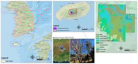
Figure 1.
Location of the study site on Jeju Island, Republic of Korea.
The conservation area on Jeju Island is characterized by high biodiversity and forms the primary ecological axis of Jeju Island. Within the study area, deciduous broad-leaved trees and Abies koreana are the dominant tree species and formed the target species for this study; they occupy 20.7% and 18.3% of the study area, respectively. However, the forest ecosystems have undergone intensive disturbances from climate change and reclamation for urban development. Even the recent climate change has affected forest types and flora. In particular, Abies koreana is a rare endemic species on Jeju Island that is at threat from and being killed by other species as well as recent climate change [40,41,42].
2.2. Research Workflow
In this study, the identification of forest phenological characteristics and creation of a time-series of phenological changes at the species–community level was conducted in three main stages (Figure 2): (1) medium-spatial and high-temporal resolution products (Landsat OLI, Thematic Mapper (TM), MODIS MOD09GQ, and MOD13Q1) were obtained from the Google Earth Engine (GEE, https://developers.google.com/earth-engine/datasets, accessed on 2 March 2021); (2) the Landsat 30-m images were fused with the MODIS 500-m images using STARFM, to produce synthetic imagery, and an accuracy assessment through the R-square and RMSE was conducted to set the optimal parameters for STARFM; (3) NDVI images, predicted through STARFM, were then classified by referencing the forest community distribution map of the current Mount Halla Absolute Conservation Area, and the time-series was analyzed for phenological changes in growth characteristics.
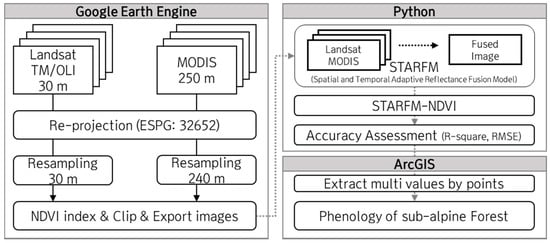
Figure 2.
Data processing workflow.
2.3. Data Collection
The method used in this study relies on high-temporal and multispectral resolution images for creating a time-series of phenological changes at the species–community level. For this, remote sensing data were obtained from the GEE platform, as it would be too time-consuming to collect sufficient data through field surveys. GEE is a cloud-based platform that enables the online processing of satellite exploration data [43]. Fast processing and results can be obtained by linking Google supercomputers with Java or Python code. Additionally, GEE reduces the data processing time and the need for advanced computers as the processing of existing satellite image data is performed online through coding.
For this study, Landsat OLI and TM products, as well as MODIS MOD09GQ and MOD13Q1 products, were obtained from GEE. Landsat 30-m resolution observations provide sufficient spatial detail for surface and change monitoring [44]. However, cloud cover and the 16-day revisit cycle of this product make it less useful for studying rapidly evolving global biophysical processes during the growing season [45]. Therefore, data fusion was attempted between Landsat and MODIS products. MODIS products are the most commonly used daily satellite imagery for observing the seasonal phenology of vegetation [46].
The Landsat TM sensor has seven bands with a spatial resolution of 30 m. MOD09GQ is a MODIS product that has undergone all atmospheric corrections and provides two surface spectrum reflectances (bands 1 and 2) with a spatial resolution of 250 m. MOD13Q1, a vegetation indices product, provides two bands: the NDVI and enhanced vegetation index, each with a spatial resolution of 250 m. NDVI is a vegetation index used to estimate vegetation vitality, productivity, and green cover rate [47]. It has been widely used for phenological detection of terrestrial ecosystems.
We obtained Landsat images with less than 10% cloud cover to minimize the influence of clouds [48,49] during 2000, 2010, and 2019, a period covering the entire growing period, and paired them with corresponding MODIS data, as shown in Table 1. Three NDVI products were constructed using bands 5 and 4 of the Landsat OLI products, bands 4 and 3 of Landsat TM products, and bands 2 and 1 of MOD09GQ. Using NDVI instead of bands allows for high-accuracy phenological analysis [31]. Both the Landsat and MODIS satellite survey data were geometrically corrected with the same coordinates (EPSG Geodetic Parameter Dataset: 32,652). Due to the characteristics of MODIS, the constructed NDVI was multiplied by 10,000, and the result was derived after downscaling to a 30-m likelihood resolution. The entire processing process was carried out on the GEE platform.

Table 1.
Data list.
2.4. Auxiliary Data
A map of forest type in the study area was acquired from the Korean Ministry of Environment. The map depicts vegetation classes (Abies koreana derived from multi-season 2015–2017 aerial imagery mapped at 20 cm resolution). The phenology was then analyzed based on the forest type map. Also, the average monthly temperatures of 2000, 2010, and 2019 were obtained from the automatic weather stations (AWS) provided by the Korean Meteorological Administration (KMA) to find the relationship between NDVI and temperature increase.
2.5. Data Fusion
Using STARFM, we fused the Landsat 30 m data with the MODIS 500 m data to generate time-series data with a high spatial resolution [31]. STARFM was chosen as the data fusion algorithm because it is the basis of other fusions and has few restrictions [38].
To increase the fusing accuracy, we minimized the influence of clouds by using 16-day composites of the MODIS data covering the prediction period [48]. Images for the same period were fused and predicted using only clean Landsat and MODIS images without clouds. For the 3 years of 2000, 2010, and 2019, a total of 54 images were fused via this method.
Using STARFM to estimate the reflectance over the fusion period assumes that the time-series change in MODIS data is the same as that in the Landsat data. Weighted combining was performed, considering the temporal, spectral, and spatial similarities of MODIS and Landsat data per pixel. We used STARFM to directly blend vegetation indices (VIs) derived from SPOT5 and MOD09Q. Several studies have found that the STARFM method performs better when directly fusing VIs than when the reflectance is fused before the VIs are calculated [50]. The value of the prediction timing for each pixel was calculated using the following equation:
where w is the size of the search window and is a parameter that determines the spatial similarity at the predicted position; W is a weight, determined according to the temporal, spectral, and spatial similarity between MODIS and Landsat data. Time similarity at the fused time is calculated using the time difference between the MODIS data and Landsat data. Spatial similarity is given a higher weight as it is closer in terms of the distance between the predicted position (the center of the search window) and the surrounding pixels. Spectral similarity is calculated by assigning a high weight to the pixels having similar spectral difference between surface reflectance of MODIS-Landsat. In this study, we used the Python code of STARFM from [51].
2.6. Parameters of STARFM
The image fusion accuracy and the time required for STARFM depend on two parameter values: the size of the search window and the number of classes classifying spectral differences between the surface reflectance of MODIS-Landsat. To improve the accuracy, it is important to determine the ideal size of the search window and the number of classes [29]. The size of the search window, which sets the areas searching for similar pixels, was set to an appropriate value through pilot prediction because, otherwise, the result may be less accurate than a certain value, depending on the target location [25]. In most studies, the size of the search window has a more direct influence on the prediction accuracy rather than the number of classes; therefore, the size of the search window will be set first, followed by the number of classes [27]. For the pilot prediction, the size of the search window and the number of classes were set by referring to the results of previous studies, and the optimal value such as window size and the number of classes was chosen in consideration of the fusion accuracy and the time required.
Two statistical criteria, the coefficient of determination (R²) and the root mean square error (RMSE), were selected to set the optimizing value of window size and the number of classes. These criteria are widely used to evaluate phenology extraction results [29,52]. They are calculated as follows:
where is the measured value, is the linear fitting value, is the average value of the measured data, and is the estimated value.
2.7. Phenological Analysis Based on Forest Types
NDVI is very effective for monitoring vegetation changes over large areas [53], and is easily calculated from satellite imagery with the following equation:
Here, NIR refers to the value of the near-infrared band, and Red refers to the value of the red-light band. NDVI ranges from −1 to 1, and values closer to 1 generally indicate higher vegetation vitality. The seasonality of local plants can be analyzed through changes in NDVI values throughout the year. NDVI image data predicted through STARFM were classified according to forest type to analyze changes in growth characteristics. The image data were classified into forest types using the ArcGIS program and based on the community distribution map of the current Mount Halla Absolute Conservation Area.
3. Results and Discussion
3.1. Results of STARFM
The two parameter values, namely the size of the search window and the number of classes, were set through pilot prediction. In accordance with previous studies [27], the pilot prediction was conducted by setting the size of the search window to 5, 10, 25, 50, 100, 150, 200, 250, and 300 [27]. As a result of the pilot prediction, when the window size was set to 50, the R2 (0.795) and RMSE (0.0402) values indicated a sufficient accuracy of the model (Figure 3a). The number of classes was set to 10, 20, 40, and 80, and the pilot prediction was carried out. The RMSEs for the different number of classes were similar, but the highest accuracy (R2 = 0.795) was obtained when the number of classes was set to 10 (Figure 3b). These STARFM accuracy evaluation results were similar to those (R2: 0.69–0.86, RMSE: 0.06–0.11) of [38] and were acceptable results. Based on the pilot prediction results, image fusion and prediction were performed with a search window of 50 and a number of classes of 10. Even though the images from the prediction period were used as 16-day composites, there was one case where a cloud existed in the prediction result. Because clouds were found mainly in the images from the summer period, the images of the summer period were excluded from later seasonality analysis.
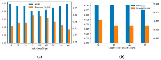
Figure 3.
Accuracy comparison of R-square and RMSE between calibrated STARFM-NDVI, Landsat NDVI when spatial and temporal adaptive reflectance fusion model (STARFM) is conducted with (a) different window sizes and (b) varying the numbers of classes.
Figure 4 shows an example of image fusion using the STARFM technique with Landsat and MODIS products. In the figure, the picture at the top left is the original MODIS product (MODIS 1 June 2000), the top right is the Landsat product (Landsat 1 June 2000) on the same date, and the bottom left is the MODIS product (MODIS 27 July 2000) on the date to be predicted by fusion. As described above, the amount of change in MODIS (1 June 2000) and MODIS (27 July 2000) was calculated, the weight of each pixel of MODIS (1 June 2000) and Landsat (1 June 2000) was calculated, and the resulting Landsat (27 July 2000) (in the lower right corner) was derived as a combination of the two.
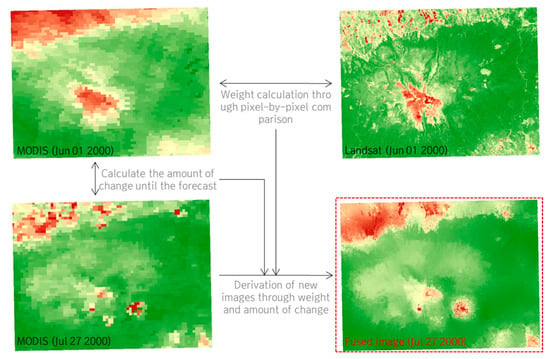
Figure 4.
Example of image fusion results using the STARFM.
3.2. Phenological Analysis
After applying STARFM to the sub-alpine area of Mount Halla, the predicted images were classified using the ArcGIS program and a community distribution map of the absolute conservation area of Mount Halla. The classification was made for eight communities, and a total of 54 × 8 = 432 fused imagery were created. Out of the eight communities, the Abies koreana and the deciduous broad-leaved forest were compared because they are the dominant types in this study area.
The results (Figure 5) showed that the time-series phenology pattern of Abies koreana had opposite characteristics to the deciduous broad-leaved forest. In the case of deciduous broad-leaved forests, the NDVI value showed a tendency to increase gradually over each season (Figure 5b). Similar to deciduous broad-leaved forests, the NDVI of Abies koreana showed a tendency to increase with each season (Figure 5a). In particular, in March and April, the average value of the total NDVI showed that the number of regions with high NDVI values gradually increased, as indicated by the average total NDVI. These results could serve as evidence to support the results of the previous study [52] that spring has higher productivity effects than fall.
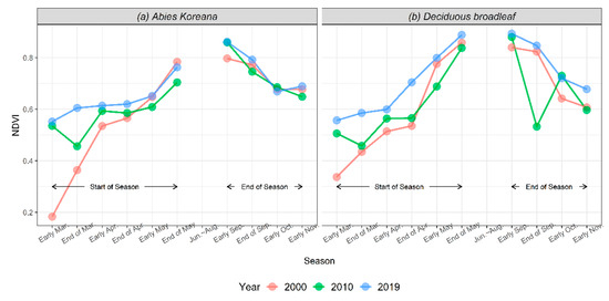
Figure 5.
Time-series of phenological change in (a) Abies koreana and (b) deciduous broadleaf forest from March to November (excluding June–August).
Deciduous broad-leaved forests generally have higher NDVI values than Abies koreana since the latter is a coniferous tree. Abies koreana showed the highest NDVI value in September due to its growth characteristics. In contrast, in 2000, the NDVI value of Abies koreana was low, and the start of the season was later than that of deciduous broad-leaved forests. Considering that Abies koreana is a coniferous tree, such an increase in NDVI is a peculiar phenomenon. These results are similar to those of previous studies [17,54] and are likely due to climate change creating a longer growing season. Therefore, for rare species like Abieas koreana, sensitive to climate change, continuous NDVI monitoring is needed to observe climate change phenomena and preserve ecosystems.
3.3. Phenology and Temperature
To examine the relationship between NDVI and temperature increase due to climate change, the average monthly temperatures in 2000, 2010, and 2019 were obtained from the AWS provided by the KMA (Figure 6). Considering the observation points in five different AWS locations around the study area, temperature data were obtained from the observatory being able to include the temporal range of this study (Figure 6a).
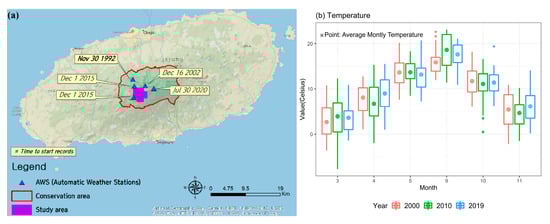
Figure 6.
(a) Locations of automatic weather stations in study area, (b) time-series graph of monthly average temperature data (data source: Korea Meteorological Administration).
The average monthly temperature increases slightly over time, except in May, where the NDVI value is relatively high. In particular, from the monthly average temperature change, the increase in average temperature occurred at the start of the season rather than at the end of the season (Figure 6b). These changes could be used as evidence to show the rise in NDVI during March and April (Figure 5). Previous studies have shown similar results [17,54], and it can be speculated that a temperature increase due to climate change can affect sensitive forest communities. In contrast, the target area also receives snow falls as much as the alpine region from late November to February. As in previous studies [55,56], phenomena and sub-alpine ecosystems are affected by the amount of snow cover and the period of cover. Furthermore, a temperature rise due to climate change affects the duration and accumulation of snow and must be observed carefully.
Through analyzing phenology by forest type in the target region (Figure 5 and Figure 6), the seasonal growing characteristics of species sensitive to climate change were confirmed, as in previous studies. In particular, the use of the STARFM technique in target sites with rainy climates sufficiently complements the qualitative limitations of Landsat data, which are heavily influenced by the weather, to increase the analytical possibilities. In addition, surface-based in situ phenological analysis provides detailed leaf development information, however, it has limitations of data availability spatially and temporally [57]. To monitor the seasonal dynamics of vegetation greenness, it is necessary to collect phenological data using remote sensing.
4. Conclusions
This study uses fusion technology to build on previous studies that have focused on time-series phenological change at a species–community level to identify phenological changes in the sub-alpine area. Our study constructed NDVI on the GEE platform using Landsat OLI and TM products with MODIS MOD09GQ and MOD13Q1 products and variables such as the coordinate system and window size. These approaches significantly reduced the time required to collect large amounts of satellite data and the uncertainty of the preprocessing method for each step. In fact, this process took only a day which included the work of coding JavaScript in the GEE platform. This process would have taken over a month if Landsat and MODIS data were downloaded from the United States Geological Survey (USGS) EarthExplorer (https://earthexplorer.usgs.gov/, accessed on 2 March 2021) to calculate NDVI. We used STARFM, which is the most widely used spatiotemporal data fusion model and shows high prediction accuracy at local scale, to fuse Landsat images for dates not covered by data, using fusion of Landsat and MODIS images. For the fusion, Landsat and MODIS data from the same period, in the form of clean images without clouds, and the forecast period data were preprocessed by reducing the effect of clouds (as much as possible) through 16-day composites. Eighteen images were predicted for each of the three years (2000, 2010, and 2019, from March to November).
Through phenological analysis in 2000, 2010, and 2019 using estimated NDVI values obtained from STARFM, we obtained three major results. First, by examining the phenology of forest types, we confirmed that NDVI values increase with time. In particular, in March and April, the average total NDVI showed that the number of regions with high NDVI values gradually increased, which indirectly confirmed that the start of season was shifting earlier. It also suggests that increasing temperature due to climate change have affected the start of season in the study regions. Second, we compared the average monthly temperatures of 2000, 2010, and 2019 to find a link to the temperature rise caused by climate change. We found that the increase in average temperature generally occurred at the start of season, rather than the end. Lastly, the STARFM technique is particularly useful for target sites with rainy climates, where the applications of Landsat data are limited by the weather. Although the climatic characteristics of the site were factored into the STARFM process, and the resulting accuracy (RMSE: 0.0402, R2: 0.795) was sufficient, it was not as high as that of other studies [58]. The phenology analysis using remote sensing techniques like STARFM is more useful to monitor the seasonal dynamics of vegetation greenness than surface-based situ phenological analysis in the perspective of data availability spatially and temporally. Additionally, the more clean, cloudless data were used, the better the results were.
In the future, this method can be supplemented by improving the image fusion process using a high-performance machine capable of processing more images. In addition, this study’s phenological analysis was only performed for specific years. It seems that it is necessary to determine the trends over multiple years to improve the accuracy and reliability of the method. Furthermore, the average value before and after the relevant year should be used, rather than just selecting a specific year. By improving the disadvantages of the mentioned data period and increasing the level of mechanical defects capable of processing large images, a phenology analysis of a wider area could be attempted as the next step in the study. Additionally, as forests respond to climate change, it would help manage the ecosystem phenology of these regions using this remote sensing technique.
Author Contributions
Conceptualization, S.-G.J. and D.-K.L.; Data curation, Y.P., Y.-W.M., D.-S.J., K.-M.P. and S.-J.P.; Methodology, S.-J.P. and S.-H.K.; Supervision, S.-G.J.; Writing—original draft, S.-J.P. All authors have read and agreed to the published version of the manuscript.
Funding
This work was supported by a grant from the National Institute of Biological Resources (NIBR), funded by the Ministry of Environment of the Republic of Korea (NIBR202002118).
Institutional Review Board Statement
Not applicable.
Informed Consent Statement
Not applicable.
Data Availability Statement
The data presented in this study are available on request from the corresponding author.
Conflicts of Interest
The authors declare no conflict of interest.
References
- IPBES. The Global Assessment Report on Biodiversity and Ecosystem Services; Secretariat of the Intergovernmental Science-Policy Platform on Biodiversity and Ecosystem Services: Bonn, Germany, 2019; Volume 172, p. 263. [Google Scholar]
- IPCC. Summary for Policy Makers. IPCC Special Report on the Impacts of Global Warming of 1.5 °C, William Solecki. 2018. Available online: http://report.ipcc.ch/sr15/pdf/sr15_spm_final.pdf (accessed on 1 November 2018).
- IPCC. Climate Change 2014: Synthesis Report. Contribution of Working Groups I, II and III to the Fifth Assessment Report of the Intergovernmental Panel on Climate Change; IPCC, Ed.; Gian-Kasper Plattner: Geneva, Switzerland, 2014; Available online: http://www.ipcc.ch (accessed on 31 October 2018).
- Warren, R.; Price, J.; Fischlin, A.; de la Nava Santos, S.; Midgley, G. Increasing impacts of climate change upon ecosystems with increasing global mean temperature rise. Clim. Chang. 2011, 106, 141–177. [Google Scholar] [CrossRef]
- Engler, R.; Randin, C.F.; Thuiller, W.; Dullinger, S.; Zimmermann, N.E.; Araújo, M.B.; Pearman, P.B.; Le Lay, G.; Piedallu, C.; Albert, C.H.; et al. 21st century climate change threatens mountain flora unequally across Europe. Glob. Chang. Biol. 2011, 17, 2330–2341. [Google Scholar] [CrossRef]
- Guisan, A.; Broennimann, O.; Buri, A.; Cianfrani, C.; D’Amen, M.; Di Cola, V.; Fernandes, R.; Gray, S.; Mateo, R.G.; Pinto, E.; et al. Climate Change Impacts on Mountain Biodiversity. Biodiversity and Climate Change; Yale University Press: London, UK, 2019; pp. 221–233. [Google Scholar]
- Huss, M.; Bookhagen, B.; Huggel, C.; Jacobsen, D.; Bradley, R.S.; Clague, J.J.; Vuille, M.; Buytaert, W.; Cayan, D.R.; Greenwood, G.; et al. Toward mountains without permanent snow and ice. Earth’s Future 2017, 5, 418–435. [Google Scholar] [CrossRef]
- Körner, C. Alpine Plant Life: Functional Plant Ecology of High Mountain Ecosystems with 47 Tables; Springer Science & Business Media: New York, NY, USA, 2003. [Google Scholar]
- Sala, O.E.; Chapin, F.S.; Armesto, J.J.; Berlow, E.; Bloomfield, J.; Dirzo, R.; Huber-Sanwald, E.; Huenneke, L.F.; Jackson, R.B.; Kinzig, A.; et al. Global biodiversity scenarios for the year 2100. Science 2000, 287, 1770–1774. [Google Scholar] [CrossRef]
- Krieger, D.J. Economic Value of Forest Ecosystem Services: A Review; The Wilderness Society: Washington, DC, USA, 2001. [Google Scholar]
- Urban, M.C.; Bocedi, G.; Hendry, A.P.; Mihoub, J.B.; Pe’er, G.; Singer, A.; Bridle, J.R.; Crozier, L.G.; De Meester, L.; Godsoe, W.; et al. Improving the forecast for biodiversity under climate change. Science 2016, 353. [Google Scholar] [CrossRef] [PubMed]
- Xiong, J.; Thenkabail, P.S.; Tilton, J.C.; Gumma, M.K.; Teluguntla, P.; Oliphant, A.; Congalton, R.G.; Yadav, K.; Gorelick, N. Nominal 30-m cropland extent map of continental Africa by integrating pixel-based and object-based algorithms using Sentinel-2 and Landsat-8 data on google earth engine. Remote Sens. 2017, 9, 65. [Google Scholar] [CrossRef]
- Hu, Y.; Hu, Y. Land cover changes and their driving mechanisms in Central Asia from 2001 to 2017 supported by Google Earth Engine. Remote Sens. 2019, 11, 554. [Google Scholar] [CrossRef]
- Naboureh, A.; Li, A.; Bian, J.; Lei, G.; Amani, M. A hybrid data balancing method for classification of imbalanced training data within google earth engine: Case studies from mountainous regions. Remote Sens. 2020, 12, 3301. [Google Scholar] [CrossRef]
- Fassnacht, F.E.; Latifi, H.; Stereńczak, K.; Modzelewska, A.; Lefsky, M.; Waser, L.T.; Straub, C.; Ghosh, A. Review of studies on tree species classification from remotely sensed data. Remote Sens. Environ. 2016, 186, 64–87. [Google Scholar] [CrossRef]
- Karahan, G.; Erşahin, S. Geostatistical analysis of spatial variation in forest ecosystems. Eurasian J. For. Sci. 2018, 6, 9–22. [Google Scholar]
- Badeck, F.W.; Bondeau, A.; Böttcher, K.; Doktor, D.; Lucht, W.; Schaber, J.; Sitch, S. Responses of spring phenology to climate change. New Phytol. 2004, 162, 295–309. [Google Scholar] [CrossRef]
- Piao, S.; Fang, J.; Zhou, L.; Ciais, P.; Zhu, B. Variations in satellite-derived phenology in China’s temperate vegetation. Glob. Chang. Biol. 2006, 12, 672–685. [Google Scholar] [CrossRef]
- Yu, L.; Yan, Z.; Zhang, S. Forest Phenology Shifts in Response to Climate Change over China–Mongolia–Russia International Economic Corridor. Forests 2020, 11, 757. [Google Scholar] [CrossRef]
- Biswas, S.; Huang, Q.; Anand, A.; Mon, M.S.; Arnold, F.E.; Leimgruber, P. A multi sensor approach to forest type mapping for advancing monitoring of sustainable development goals (SDG) in Myanmar. Remote Sens. 2020, 12, 3220. [Google Scholar] [CrossRef]
- Nguyen, L.H.; Joshi, D.R.; Clay, D.E.; Henebry, G.M. Characterizing land cover/land use from multiple years of Landsat and MODIS time series: A novel approach using land surface phenology modeling and random forest classifier. Remote Sens. Environ. 2020, 238, 111017. [Google Scholar] [CrossRef]
- Pu, R.; Bell, S. Mapping seagrass coverage and spatial patterns with high spatial resolution IKONOS imagery. International J. Appl. Earth Obs. Geoinf. 2017, 54, 145–158. [Google Scholar] [CrossRef]
- Ogilvie, A.; Belaud, G.; Massuel, S.; Mulligan, M.; Le Goulven, P.; Calvez, R. Surface water monitoring in small water bodies: Potential and limits of multi-sensor Landsat time series. Hydrol. Earth Syst. Sci. Discuss. 2018, 1–35. [Google Scholar] [CrossRef]
- Scarth, P.; Armston, J.; Lucas, R.; Bunting, P. A Structural Classification of Australian Vegetation Using ICESat/GLAS, ALOS PALSAR, and Landsat Sensor Data. Remote Sens. 2019, 11, 147. [Google Scholar] [CrossRef]
- Kim, Y.; No-Wook, P. Comparison of Spatio-temporal Fusion Models of Multiple Satellite Images for Vegetation Monitoring. Korean J. Remote Sens. 2019, 35, 1209–1219. [Google Scholar]
- Gao, F.; Masek, J.; Schwaller, M.; Hall, F. On the blending of the Landsat and MODIS surface reflectance: Predict daily Landsat surface reflectance. IEEE Trans. Geosci. Remote Sens. 2006, 44, 2207–2218. [Google Scholar]
- Gevaert, C.M.; García-Haro, F.J. A comparison of STARFM and an unmixing-based algorithm for Landsat and MODIS data fusion. Remote Sens. Environ. 2015, 156, 34–44. [Google Scholar] [CrossRef]
- Emelyanova, I.V.; McVicar, T.R.; Van Niel, T.G.; Li, L.T.; Van Dijk, A.I. Assessing the accuracy of blending Landsat–MODIS surface reflectances in two landscapes with contrasting spatial and temporal dynamics: A framework for algorithm selection. Remote Sens. Environ. 2013, 133, 193–209. [Google Scholar] [CrossRef]
- Cui, J.; Zhang, X.; Luo, M. Combining linear pixel unmixing and STARFM for spatiotemporal fusion of Gaofen-1wide field of view imagery and MODIS imagery. Remote Sens. 2018, 10, 1047. [Google Scholar] [CrossRef]
- Swain, R.; Sahoo, B. Mapping of Heavy Metal Pollution in River Water at Daily Time-Scale Using Spatio-Temporal Fusion of MODIS-Aqua and Landsat Satellite Imageries. J. Environ. Manag. 2017, 192, 1–14. [Google Scholar] [CrossRef]
- Walker, J.J.; De Beurs, K.M.; Wynne, R.H.; Gao, F. Evaluation of Landsat and MODIS data fusion products for analysis of dryland forest phenology. Remote Sens. Environ. 2012, 117, 381–393. [Google Scholar] [CrossRef]
- Singh, D. Generation and evaluation of gross primary productivity using Landsat data through blending with MODIS data. Int. J. Appl. Earth Obs. Geoinf. 2011, 13, 59–69. [Google Scholar] [CrossRef]
- Gordo, O.; Sanz, J.J. Impact of climate change on plant phenology in Mediterranean ecosystems. Glob. Chang. Biol. 2010, 16, 1082–1106. [Google Scholar] [CrossRef]
- Du, J.; He, Z.; Yang, J.; Chen, L.; Zhu, X. Detecting the effects of climate change on canopy phenology in coniferous forests in semi-arid mountain regions of China. Int. J. Remote Sens. 2014, 35, 6490–6507. [Google Scholar] [CrossRef]
- Madonsela, S.; Cho, M.A.; Mathieu, R.; Mutanga, O.; Ramoelo, A.; Kaszta, Ż.; Van De Kerchove, R.V.; Wolff, E. Multi-phenology WorldView-2 imagery improves remote sensing of savannah tree species. Int. J. Appl. Earth Obs. Geoinf. 2017, 58, 65–73. [Google Scholar] [CrossRef]
- Yan, J.; Zhou, W.; Han, L.; Qian, Y. Mapping vegetation functional types in urban areas with WorldView-2 imagery: Integrating object-based classification with phenology. Urban For. Urban Green. 2018, 31, 230–240. [Google Scholar] [CrossRef]
- Melaas, E.K.; Friedl, M.A.; Zhu, Z. Detecting Interannual Variation in Deciduous Broadleaf Forest Phenology Using Landsat TM/ETM+ Data. Remote Sens. Environ. 2013, 132, 176–185. [Google Scholar] [CrossRef]
- Zheng, Y.; Wu, B.; Zhang, M.; Zeng, H. Crop Phenology Detection Using High Spatio-Temporal Resolution Data Fused from SPOT5 and MODIS Products. Sensors 2016, 16, 2099. [Google Scholar] [CrossRef] [PubMed]
- Jeju Regional Office of Meteorology. 2019 Jeju Island Climate Data Collection; Jeju Regional Office of Meteorology: Jeju, Korea, 2019. [Google Scholar]
- Hwang, J.E.; Kim, Y.J.; Shin, M.H.; Hyun, H.J.; Bohnert, H.J.; Park, H.C. A comprehensive analysis of the Korean fir (Abies koreana) genes expressed under heat stress using transcriptome analysis. Sci. Rep. 2018, 8. [Google Scholar] [CrossRef]
- Koo, K.A.; Kong, W.S.; Park, S.U.; Lee, J.H.; Kim, J.; Jung, H. Sensitivity of Korean fir (Abies koreana Wils.), a threatened climate relict species, to increasing temperature at an island subalpine area. Ecol. Model. 2017, 353, 5–16. [Google Scholar] [CrossRef]
- Kim, D.W.; Park, D.Y.; Jeong, D.Y.; Park, H.C. Identification of Molecular Markers for Population Diagnosis of Korean Fir (Abies koreana) Vulnerable to Climate Change. Proc. Natl. Inst. Ecol. 2020, 1, 68–73. [Google Scholar]
- Gorelick, N.; Hancher, M.; Dixon, M.; Ilyushchenko, S.; Thau, D.; Moore, R. Google Earth Engine: Planetary-scale geospatial analysis for everyone. Remote Sens. Environ. 2017, 202, 18–27. [Google Scholar] [CrossRef]
- Zhou, Y.; Dong, J.; Liu, J.; Metternicht, G.; Shen, W.; You, N.; Zhao, G.; Xiao, X. Are there sufficient Landsat observations for retrospective and continuous monitoring of land cover changes in China? Remote Sens. 2019, 11, 1808. [Google Scholar] [CrossRef]
- Roy, D.P.; Ju, J.; Lewis, P.; Schaaf, C.; Gao, F.; Hansen, M.; Lindquist, E. Multi-temporal MODIS-Landsat data fusion for relative radiometric normalization, gap filling, and prediction of Landsat data. Remote Sens. Environ. 2008, 112, 3112–3130. [Google Scholar] [CrossRef]
- Suepa, T.; Qi, J.; Lawawirojwong, S.; Messina, J.P. Understanding spatio-temporal variation of vegetation phenology and rainfall seasonality in the monsoon Southeast Asia. Environ. Res. 2016, 147, 621–629. [Google Scholar] [CrossRef] [PubMed]
- Rouse, J.W., Jr.; Haas, R.; Schell, J.; Deering, D. Monitoring Vegetation Systems in the Great Plains with Erts; NASA Special Publication: Washington, DC, USA, 1974; Volume 351, p. 309. [Google Scholar]
- Testa, S.; Mondino, E.C.B.; Pedroli, C. Correcting MODIS 16-day composite NDVI time-series with actual acquisition dates. Eur. J. Remote Sens. 2014, 47, 285–305. [Google Scholar] [CrossRef]
- Karlsen, S.R.; Anderson, H.B.; Van Der Wal, R.; Hansen, B.B. A new NDVI measure that overcomes data sparsity in cloud-covered regions predicts annual variation in ground-based estimates of high arctic plant productivity. Environ. Res. Lett. 2018, 13. [Google Scholar] [CrossRef]
- Jarihani, A.A.; McVicar, T.R.; van Niel, T.G.; Emelyanova, I.V.; Callow, J.N.; Johansen, K. Blending landsat and MODIS data to generate multispectral indices: A comparison of “index-then-blend” and “Blend-Then-Index” approaches. Remote Sens. 2014, 6, 9213–9238. [Google Scholar] [CrossRef]
- Mileva, N.; Mecklenburg, S.; Gascon, F. New tool for spatio-temporal image fusion in remote sensing: A case study approach using Sentinel-2 and Sentinel-3 data. Image Signal Process. Remote Sens. 2018, 10789. [Google Scholar] [CrossRef]
- Richardson, A.D.; Black, T.A.; Ciais, P.; Delbart, N.; Friedl, M.A.; Gobron, N.; Hollinger, D.Y.; Kutsch, W.L.; Longdoz, B.; Luyssaert, S.; et al. Influence of Spring and Autumn Phenological Transitions on Forest Ecosystem Productivity. Philos. Trans. R. Soc. Lond. B 2010, 365, 3227–3246. [Google Scholar] [CrossRef] [PubMed]
- Kim, D.; Park, J.; Jang, D. Analysis of the Possibility for Drought Detection of Spring Season Using SPI and NDVI. J. Assoc. Korean Geogr. 2017, 6, 165–174. [Google Scholar]
- Liu, M.; Liu, X.; Dong, X.; Zhao, B.; Zou, X.; Wu, L.; Wei, H. An improved spatiotemporal data fusion method using surface heterogeneity information based on estarfm. Remote Sens. 2020, 12, 3673. [Google Scholar] [CrossRef]
- Xie, J.; Kneubühler, M.; Garonna, I.; Notarnicola, C.; De Gregorio, L.; De Jong, R.; Chimani, B.; Schaepman, M.E. Altitude-Dependent Influence of Snow Cover on Alpine Land Surface Phenology. J. Geophys. Res. Biogeosci. 2017, 122, 1107–1122. [Google Scholar] [CrossRef]
- Xie, J.; Kneubühler, M.; Garonna, I.; de Jong, R.; Notarnicola, C.; De Gregorio, L.; Schaepman, M.E. Relative Influence of Timing and Accumulation of Snow on Alpine Land Surface Phenology. J. Geophys. Res. Biogeosci. 2018, 123, 561–576. [Google Scholar] [CrossRef]
- Cleland, E.E.; Chuine, I.; Menzel, A.; Mooney, H.A.; Schwartz, M.D. Shifting Plant Phenology in Response to Global Change. Trends Ecol. Evol. 2007, 22, 357–365. [Google Scholar] [CrossRef] [PubMed]
- Hatfield, J.L.; Prueger, J.H. Temperature extremes: Effect on plant growth and development. Weather Clim. Extrem. 2015, 10, 4–10. [Google Scholar] [CrossRef]
Publisher’s Note: MDPI stays neutral with regard to jurisdictional claims in published maps and institutional affiliations. |
© 2021 by the authors. Licensee MDPI, Basel, Switzerland. This article is an open access article distributed under the terms and conditions of the Creative Commons Attribution (CC BY) license (http://creativecommons.org/licenses/by/4.0/).