
Estimating Biomass and Carbon Storage by Georgia Forest Types and Species Groups Using the FIA Data Diameters, Basal Areas, Site Indices, and Total Heights


Abstract
:1. Introduction
2. Materials and Methods
2.1. Study Site, Biomass, Forest Types, and Species Groups
2.2. Data Acquisition
2.3. Biomass Estimation
2.3.1. Biomass Per Tree
2.3.2. Total Biomass Calculations
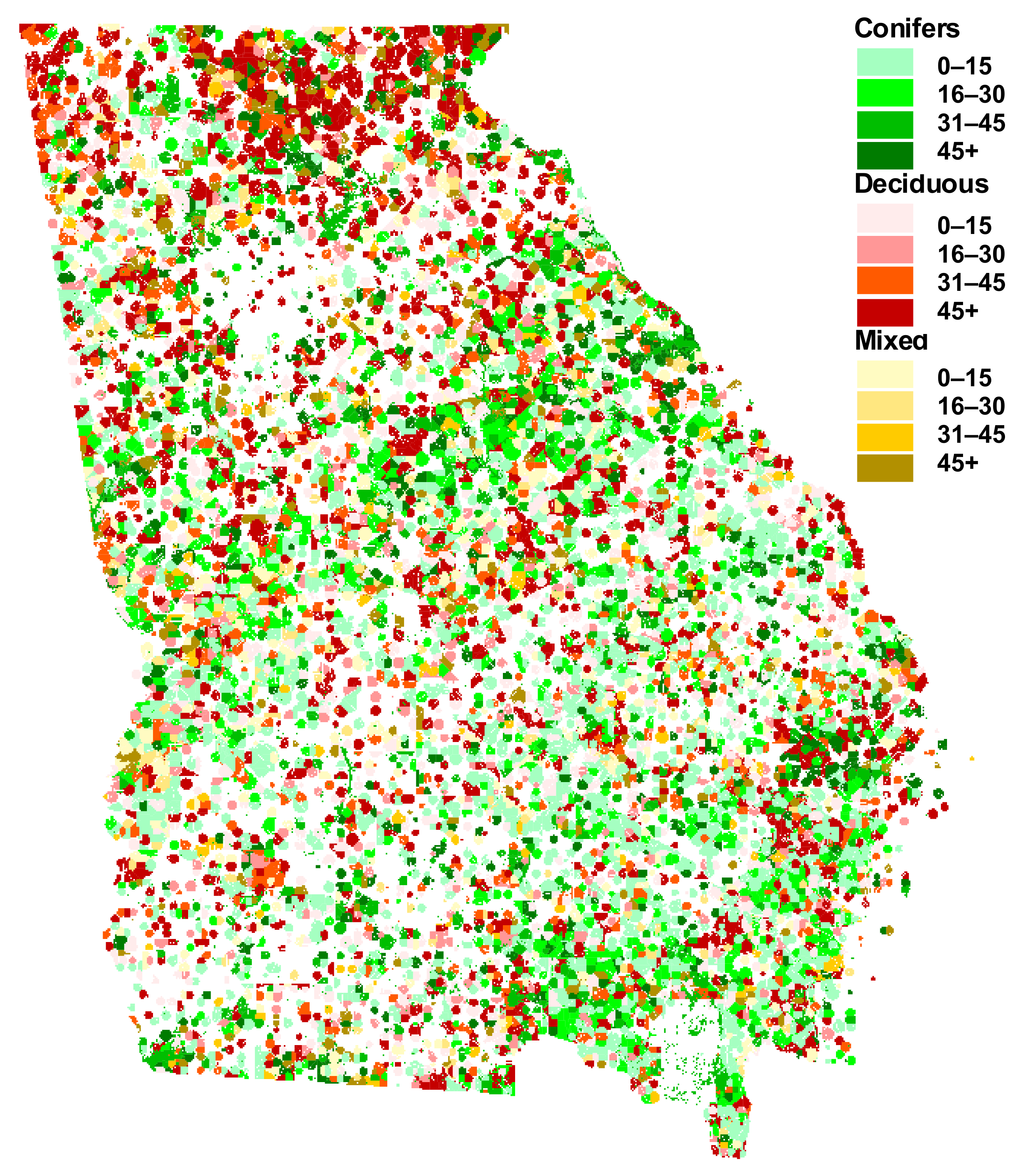
2.4. Visualization of the Estimated Biomass and Carbon Quantities
3. Results
4. Discussion and Conclusions
Author Contributions
Funding
Acknowledgments
Conflicts of Interest
Appendix A

| FIA Species Groups | Coefficients | |||||
|---|---|---|---|---|---|---|
| a | b | c | d | f | g | |
| Jack pine | 16.934 | −0.12972 | 1 | 0.20854 | 0.77792 | 0.12902 |
| Red pine | 36.851 | −0.08298 | 1 | 0.00001 | 0.63884 | 0.18231 |
| Eastern white pine | 16.281 | −0.08621 | 1 | 0.1622 | 0.86833 | 0.23316 |
| Ponderosa pine | 36.851 | −0.08298 | 1 | 0.00001 | 0.63884 | 0.18231 |
| White spruce | 31.957 | −0.18511 | 1.702 | 0 | 0.68967 | 0.162 |
| Black spruce | 20.038 | −0.18981 | 1.2909 | 0.17836 | 0.57343 | 0.10159 |
| Balsam fir | 14.304 | −0.19894 | 1.4195 | 0.23349 | 0.76878 | 0.12399 |
| Hemlock | 5.3117 | −0.10357 | 1 | 0.68454 | 0.7141 | 0 |
| Eastern cedar, other cedars | 8.2079 | −0.19672 | 1.3112 | 0.33978 | 0.76173 | 0.11666 |
| Other softwoods | 16.934 | −0.12972 | 1 | 0.20854 | 0.77792 | 0.12902 |
| Select white oak, white oak | 9.2078 | −0.22208 | 1 | 0.31723 | 0.8256 | 0.13465 |
| Select red oak | 6.6844 | −0.19049 | 1 | 0.43972 | 0.82962 | 0.10806 |
| Other red oak | 3.8011 | −0.39213 | 2.9053 | 0.55634 | 0.84317 | 0.09593 |
| Select hickory | 6.1034 | −0.17368 | 1 | 0.44725 | 1.0237 | 0.1461 |
| Basswood | 6.3628 | −0.27859 | 1.8677 | 0.49589 | 0.76169 | 0.05841 |
| Beech | 7.1852 | −0.28384 | 1.4417 | 0.38884 | 0.82157 | 0.11411 |
| Hard maple | 5.3416 | −0.23044 | 1.1529 | 0.54194 | 0.8344 | 0.06372 |
| Soft maple | 6.68 | −0.27725 | 1.4287 | 0.40115 | 0.85299 | 0.12403 |
| Elm | 8.458 | −0.27527 | 1.9602 | 0.34894 | 0.89213 | 0.12594 |
| Black ash | 11.291 | −0.2525 | 1.5466 | 0.35711 | 0.7506 | 0.06859 |
| White ash, green ash | 8.1782 | −0.27316 | 1.725 | 0.38694 | 0.75822 | 0.10847 |
| Sycamore | 6.3628 | −0.27859 | 1.8677 | 0.49589 | 0.76169 | 0.05841 |
| Cottonwood, willow | 13.625 | −0.28668 | 1.6124 | 0.30651 | 1.0292 | 0.0746 |
| Balsam poplar, quaking aspen | 6.4301 | −0.23545 | 1.338 | 0.4737 | 0.73385 | 0.08228 |
| Bigtooth aspen | 5.5346 | −0.22637 | 1 | 0.46918 | 0.72456 | 0.11782 |
| River birch, paper birch | 7.2773 | −0.22721 | 1 | 0.41179 | 0.76498 | 0.11046 |
| Black cherry | 5.3416 | −0.23044 | 1.1529 | 0.54194 | 0.8344 | 0.06372 |
| Yl. Pop, Butternut, bl. walnut, | 6.3628 | −0.27859 | 1.8677 | 0.49589 | 0.76169 | 0.05841 |
| Other hardwoods | 6.9572 | −0.26564 | 1 | 0.4866 | 0.76954 | 0.01618 |
| FIA Species Group | Species | Biomass Type | Reference | a | b |
|---|---|---|---|---|---|
| 110 | Shortleaf pine | Dry without foliage | [18] | −1.55499 | 1.12266 |
| Dry including foliage | [18] | −1.52244 | 1.11886 | ||
| Dry foliage | [18] | −2.61282 | 1.03712 | ||
| Green without foliage | [18] | −1.25376 | 1.12517 | ||
| Green including foliage | [18] | −1.20938 | 1.11931 | ||
| Green foliage | [18] | −2.11074 | 1.01076 | ||
| 131 | Loblolly pine | Dry without foliage | [21] | −1.072 | 0.99421 |
| Dry including foliage | [21] | −1.0293 | 0.98788 | ||
| Dry foliage | [21] | −1.87201 | 0.84237 | ||
| Green without foliage | [21] | −0.83678 | 1.01136 | ||
| Green including foliage | [21] | −0.78974 | 1.00404 | ||
| Green foliage | [21] | −1.54968 | 0.83959 | ||
| 121 | Longleaf pine | Dry without foliage | [13] | −1.15588 | 1.027 |
| (DBH3 5 inches) | Dry including foliage | [13] | −1.06186 | 1.00853 | |
| Green without foliage | [13] | −0.75522 | 1.00514 | ||
| Green including foliage | [13] | −0.64745 | 0.98442 | ||
| 121 | Longleaf pine | Dry without foliage | [13] | −0.71944 | 0.88503 |
| (DBH < 5 inches) | Dry including foliage | [13] | −0.65729 | 0.88019 | |
| Green without foliage | [13] | −0.31359 | 0.85584 | ||
| Green including foliage | [13] | −0.24556 | 0.85263 | ||
| 111 | Slash pine | Dry without foliage | [22] | −1.20931 | 1.0431 |
| Dry including foliage | [22] | −1.16061 | 1.03527 | ||
| Dry foliage | [22] | −1.90538 | 0.85834 | ||
| Green without foliage | [22] | −0.93767 | 1.03929 | ||
| Green including foliage | [22] | −0.88096 | 1.03014 | ||
| Green foliage | [22] | −1.54455 | 0.84989 | ||
| Other softwoods | as Slash pine | All | [22] | As above | As above |
| FIA Species Group | Species | Biomass type | Reference | A | b | c |
|---|---|---|---|---|---|---|
| 812 | Southern red oak | Dry without foliage | [24] | 0.06707 | 0.96117 | |
| (DBH < 11 inches) | Dry including foliage | [24] | 0.07361 | 0.95348 | ||
| Green without foliage | [24] | 0.12015 | 0.95457 | |||
| Green including foliage | [24] | 0.13815 | 0.94228 | |||
| 812 | Southern red oak | Dry without foliage | [24] | 0.0277 | 1.14557 | 0.96117 |
| (DBH3 11 inches) | Dry including foliage | [24] | 0.0281 | 1.15418 | 0.95348 | |
| Green without foliage | [24] | 0.04601 | 1.15471 | 0.95457 | ||
| Green including foliage | [24] | 0.04665 | 1.16866 | 0.94228 | ||
| 611 | Sweetgum | Dry without foliage | [24] | 0.049 | 0.94648 | |
| (DBH < 11 inches) | Dry including foliage | [24] | 0.05152 | 0.94351 | ||
| Green without foliage | [24] | 0.10528 | 0.94503 | |||
| Green including foliage | [24] | 0.1155 | 0.9383 | |||
| 611 | Sweetgum | Dry without foliage | [24] | 0.01278 | 1.22662 | 0.94648 |
| (DBH3 11 inches) | Dry including foliage | [24] | 0.01409 | 1.2138 | 0.94351 | |
| Green without foliage | [24] | 0.03175 | 1.19494 | 0.94503 | ||
| Green including foliage | [24] | 0.03517 | 1.18624 | 0.9383 | ||
| 621 | Yellow poplar | Dry without foliage | [24] | 0.0522 | 0.95352 | |
| (DBH < 11 inches) | Dry including foliage | [24] | 0.05583 | 0.9482 | ||
| Green without foliage | [24] | 0.11943 | 0.93782 | |||
| Green including foliage | [24] | 0.13684 | 0.92608 | |||
| 621 | Yellow poplar | Dry without foliage | [24] | 0.03109 | 1.06155 | 0.95352 |
| (DBH3 11 inches) | Dry including foliage | [24] | 0.03296 | 1.05809 | 0.9482 | |
| Green without foliage | [24] | 0.06298 | 1.07125 | 0.93782 | ||
| Green including foliage | [24] | 0.06819 | 1.07131 | 0.92608 | ||
| 691 | Tupelo | Dry without foliage | [23] | 0.05548 | 0.92453 | |
| Dry including foliage | [23] | 0.05696 | 0.92338 | |||
| Green without foliage | [23] | 0.11048 | 0.9211 | |||
| Green including foliage | [23] | 0.11539 | 0.91882 | |||
| 693 | Blackgum | Dry without foliage | [23] | 0.07011 | 0.93057 | |
| (DBH < 11 inches) | Dry including foliage | [23] | 0.07335 | 0.92799 | ||
| Green without foliage | [23] | 0.11712 | 0.94824 | |||
| Green including foliage | [23] | 0.12331 | 0.94557 | |||
| 693 | Blackgum | Dry without foliage | [23] | 0.02912 | 1.11381 | 0.93057 |
| (DBH3 11 inches) | Dry including foliage | [23] | 0.0302 | 1.11305 | 0.92799 | |
| Green without foliage | [23] | 0.0536 | 1.11125 | 0.94824 | ||
| Green including foliage | [23] | 0.05576 | 1.11106 | 0.94557 | ||
| 802 | White oak | Dry without foliage | [24] | 0.05928 | 0.98979 | |
| (DBH < 11 inches) | Dry including foliage | [24] | 0.0612 | 0.98969 | ||
| Green without foliage | [24] | 0.10312 | 0.98415 | |||
| Green including foliage | [24] | 0.10895 | 0.98258 | |||
| 802 | White oak | Dry without foliage | [24] | 0.02926 | 1.13699 | 0.98979 |
| (DBH3 11 inches) | Dry including foliage | [24] | 0.03071 | 1.13346 | 0.98969 | |
| Green without foliage | [24] | 0.0437 | 1.16321 | 0.98415 | ||
| Green including foliage | [24] | 0.05143 | 1.15748 | 0.98258 | ||
| Other hardwoods | Dry without foliage | [24] | 0.06679 | 0.94275 | ||
| (DBH < 11 inches) | Dry including foliage | [24] | 0.07153 | 0.938 | ||
| Green without foliage | [24] | 0.12327 | 0.94274 | |||
| Green including foliage | [24] | 0.13901 | 0.93307 | |||
| Other hardwoods | Dry without foliage | [24] | 0.02252 | 1.16948 | 0.94275 | |
| (DBH3 11 inches) | Dry including foliage | [24] | 0.02366 | 1.16867 | 0.938 | |
| Green without foliage | [24] | 0.04038 | 1.17543 | 0.94274 | ||
| Green including foliage | [24] | 0.04279 | 1.17874 | 0.933137 |
References
- Alexeyev, V.A.; Birdsey, R.A. Carbon Storage in Forests and Peatlands of Russia; General Technical Report NE-244; U.S. Department of Agriculture, Forest Service, Northeastern Forest Experiment Station: Radnor, PA, USA, 1998; p. 137. [Google Scholar]
- Birdsey, R.A. Carbon Storage and Accumulation in United States Forest Ecosystems; General Technical Report, WO-59; U.S. Department of Agriculture, Forest Service: Washington, DC, USA, 1992; p. 51. [Google Scholar]
- Detwiler, R.P.; Hall, C.A.S. Tropical forests and the global carbon cycle. Science 1988, 239, 42–47. [Google Scholar] [CrossRef] [PubMed]
- Reams, G.A.; Roesch, F.A.; Cost, N.D. Annual Forest Inventory—Cornerstone of Sustainability in the South. J. For. 1999, 97, 21–26. [Google Scholar]
- Liu, S.; Cieszewski, C. Impacts of Management Intensity and Harvesting Practices on Long-term Forest Resource Sustainability in Georgia. Math. Comput. For. Nat. Resour. Sci. 2009, 1, 52–66. Available online: http://mcfns.net/index.php/Journal/article/view/MCFNS.1-52 (accessed on 21 January 2021).
- Cieszewski, C.J.; Borders, B.; Whiffen, H.; Harrison, W.M. Forest Inventory in Georgia. In Proceedings of the IUFRO Conference on Remote Sensing and Forest Monitoring, Rogów, Poland, 1–3 June 1999. [Google Scholar]
- Cost, N.D.; Howard, J.O.; Mead, B.; McWilliams, W.H.; Smith, W.B.; Van Hooser, D.D.; Wharton, E.H. The Forest Biomass Resource of the United States; General Research Paper WO-57; USDA Forest Service: Washington, DC, USA, 1990; p. 21. [Google Scholar]
- Cost, N.D.; Tansey, J.B. Multiresource Inventories: Woody Biomass in Georgia; Research Paper SE-248; U.S. Department of Agriculture, Forest Service, Southeastern Forest Experiment Station: Asheville, NC, USA, 1985; p. 32. [Google Scholar]
- Thompson, M.T. Forest Statistics for Georgia, 1997; Resource Bulletin SRS-36; USDA Forest Service, Southern Forest Experiment Station: Asheville, NC, USA, 1998; p. 93. [Google Scholar]
- Brown, S.L.; Schroeder, P.; Kern, J.S. Spatial distribution of biomass in forests of the eastern USA. For. Ecol. Manag. 1999, 123, 81–90. [Google Scholar] [CrossRef]
- Schroeder, P.; Brown, S.L.; Mo, J.; Birdsey, R.A.; Cieszewski, C.J. Biomass estimation for temperate broadleaf forests of the US using forest inventory data. For. Sci. 1997, 43, 424–434. [Google Scholar]
- Brown, S.L.; Schroeder, P.; Birdsey, R.A. Aboveground biomass distribution of US eastern hardwood forests and the use of large trees as an indicator of forest development. For. Ecol. Manag. 1997, 96, 37–47. [Google Scholar] [CrossRef]
- Baldwin, V.C.; Saucier, J.R. Aboveground Weight and Volume of Unthinned, Planted Longleaf Pine on West Gulf Forest Sites; Research Paper SO-191; U.S. Department of Agriculture, Forest Service, Southern Forest Experiment Station: New Orleans, LA, USA, 1983; p. 25. [Google Scholar]
- Hansen, M.H.; Frieswyk, T.; Glover, J.F.; Kelly, J.F. The Eastwide Forest Inventory Database: Users Manual; General Technical Report NC-151; U.S. Department of Agriculture, Forest Service, North Central Forest Experiment Station: St. Paul, MN, USA, 1992; p. 48. [Google Scholar]
- Miles, P.D.; Brand, G.J.; Alerich, C.L.; Bednar, L.F.; Woudenberg, S.W.; Glover, J.F.; Ezzell, E.N. The Forest Inventory and Analysis Database: Database Description and User’s Manual Version 1.0 Revision 8. 2001. Available online: http://www.ncrs.fs.fed.us/4801/FIADB/fiadb_documentation/FIADB_DOCUMENTATION.htm (accessed on 1 June 2001).
- Cairns, M.A.; Brown, S.; Helmer, E.H.; Baumgardner, G.A. Root biomass allocation in the world’s upland forests. Oecologia 1997, 111, 1–11. [Google Scholar] [CrossRef] [PubMed]
- Lowe, R.; Cieszewski, C. Multi-Source K-Nearest Neighbor, Mean Balanced Forest Inventory of Georgia. Math. Comput. For. Nat. Resour. Sci. 2014, 6, 65–79. Available online: http://mcfns.net/index.php/Journal/article/view/6_65 (accessed on 21 January 2021).
- Clark, A., III; Taras, M.A. Biomass of Shortleaf Pine in a Natural Sawtimber Stand in Northern Mississippi; Research Paper SE-146; USDA Forest Service, Southeastern Forest Experiment Station: Asheville, NC, USA, 1976; p. 32. [Google Scholar]
- Keays, J.L. Full-tree and complete-tree utilization for pulp and paper. For. Prod. J. 1974, 24, 13–16. [Google Scholar]
- Parresol, B.R. Assessing Tree and Stand Biomass: A Review with Examples and, Critical Comparisons. For. Sci. 1999, 45, 573–593. [Google Scholar]
- Taras, M.A.; Clark, A., III. Aboveground biomass of loblolly pine in a natural, uneven-aged sawtimber stand in central Alabama. Tappi 1975, 58, 103–105. [Google Scholar]
- Taras, M.A.; Phillips, D.R. Aboveground Biomass of Slash Pine in a Natural Sawtimber Stand in Southern Alabama; Research Paper SE-188; USDA Forest Service, Southeastern Forest Experiment Station: Asheville, NC, USA, 1978; p. 31. [Google Scholar]
- Clark, A., III; Phillips, D.R.; Frederick, D.J. Weight, Volume and Physical Properties of Major Hardwood Species in the Gulf and Atlantic Coastal Plain; Research Paper SE-250; USDA Forest Service, Southeastern Forest Experiment Station: Asheville, NC, USA, 1985; p. 66. [Google Scholar]
- Clark, A., III; Phillips, D.R.; Frederick, D.J. Weight, Volume and Physical Properties of Major Hardwood Species in the Piedmont; Research Paper SE-255; USDA Forest Service, Southeastern Forest Experiment Station: Asheville, NC, USA, 1986; p. 78. [Google Scholar]
- Woudenberg, S.W.; Farrenkopf, T.O. The Westwide Forest Inventory Data Base: User’s Manual; General Technical Report INT-GTR-317; U.S. Department of Agriculture, Forest Service, Intermountain Research Station: Ogden, UT, USA, 1995; p. 67. [Google Scholar]
- Brown, S.L. Estimating Biomass and Biomass Change in Tropical Forests: A Primer; FAO Forestry Paper 134; Food and Agriculture Organization: Rome, Italy, 1997. [Google Scholar]
- McClure, J.P.; Saucier, J.R.; Biesterfeldt, R.C. Biomass in Southeastern Forests; Research Paper SE-227; USDA Forest Service, Southeastern Forest Experiment Station: Asheville, NC, USA, 1981; p. 38. [Google Scholar]
- Adegbidi, H.G.; Jokela, E.J.; Comerford, N.B.; Barros, N.F. Biomass development for intensively managed loblolly pine plantations growing on Spodosols in the southeastern USA. For. Ecol. Manag. 2002, 167, 91–102. [Google Scholar] [CrossRef]
- Carmean, W.H.; Hanh, J.T.; Jacobs, R.D. Site Index Curves for Forest Tree Species in the Eastern United States; General Technical Report NC-128; St. USDA Forest Service, North Central Forest Experiment Station: Paul, MN, USA, 1989; p. 142. [Google Scholar]
- Hahn, J.T. Tree Volume and Biomass Equations for the Lake States; Research Paper NC-250; USDA Forest Service, North Central Forest Experiment Station: St. Paul, MN, USA, 1984; p. 10. [Google Scholar]
- Bray, J.R. Root production and the estimation of net productivity. Can. J. Bot. 1963, 41, 65–72. [Google Scholar] [CrossRef]
- Tavernia, B.; Nelson, M.; Goerndt, M.; Walters, B.; Toney, C. Changes in Forest Habitat Classes under Alternative Climate and Land-Use Change Scenarios in the Northeast and Midwest, USA. Math. Comput. For. Nat. Resour. Sci. 2013, 5, 135–150. Available online: http://mcfns.net/index.php/Journal/article/view/MCFNS_165 (accessed on 21 January 2021).
- Martell, D. The Development and Implementation of Forest and Wildland Fire Management Decision Support Systems: Reflections on Past Practices and Emerging Needs and Challenges. Math. Comput. For. Nat. Resour. Sci. 2011, 3, 18–26. Available online: http://mcfns.net/index.php/Journal/article/view/MCFNS.3-18 (accessed on 21 January 2021).


| Tree Species or Species Group | Source of Equation(s) |
|---|---|
| Shortleaf pine | [18] |
| Loblolly pine | [21] |
| Longleaf pine | [13] |
| Slash pine | [22] |
| Other pines—as slash pine | [22] |
| Hardwoods | [23,24] |
| Tree | Foliage | Roots | Total | ||||||
|---|---|---|---|---|---|---|---|---|---|
| mil. t | % | mil. t | % | mil. t | % | mil. t | % | ||
| Species groups | Hardwood | 479 | 59 | 13 | 46 | 105 | 58 | 598 | 59 |
| 496 | 59 | 14 | 47 | 107 | 58 | 617 | 58 | ||
| Softwood | 330 | 41 | 15 | 54 | 75 | 42 | 419 | 41 | |
| 348 | 41 | 16 | 53 | 80 | 42 | 444 | 42 | ||
| Forest type | Evergreen | 319 | 40 | 14 | 50 | 74 | 41 | 407 | 40 |
| 340 | 40 | 15 | 50 | 79 | 42 | 434 | 41 | ||
| Deciduous | 392 | 48 | 11 | 39 | 84 | 47 | 487 | 48 | |
| 394 | 47 | 11 | 37 | 84 | 45 | 489 | 46 | ||
| Mixed | 98 | 12 | 3 | 11 | 22 | 12 | 123 | 12 | |
| 110 | 13 | 4 | 13 | 24 | 13 | 138 | 13 | ||
| Sum of components’ dry biomass (million tons) | 809 | 79 | 28 | 3 | 180 | 18 | 1017 | 100 | |
| 844 | 79 | 30 | 3 | 187 | 18 | 1061 | 100 | ||
| Tree | Foliage | Roots | Total | ||||||
|---|---|---|---|---|---|---|---|---|---|
| Tg | % | Tg | % | Tg | % | Tg | % | ||
| Species groups | Hardwood | 239.5 | 59 | 6.5 | 46 | 52.5 | 58 | 299.0 | 59 |
| 248.0 | 59 | 7.0 | 47 | 53.5 | 58 | 308.5 | 58 | ||
| Softwood | 165.0 | 41 | 7.5 | 54 | 37.5 | 42 | 209.5 | 41 | |
| 174.0 | 41 | 8.0 | 53 | 40.0 | 42 | 222.0 | 42 | ||
| Forest type | Evergreen | 159.5 | 40 | 7.0 | 50 | 37.0 | 41 | 203.5 | 40 |
| 170.0 | 40 | 7.5 | 50 | 39.5 | 42 | 217.0 | 41 | ||
| Deciduous | 196.0 | 48 | 5.5 | 39 | 42.0 | 47 | 243.5 | 48 | |
| 197.0 | 47 | 5.5 | 37 | 42.0 | 45 | 244.5 | 46 | ||
| Mixed | 49.0 | 12 | 1.5 | 11 | 11.0 | 12 | 61.5 | 12 | |
| 55.0 | 13 | 2.0 | 13 | 12.0 | 13 | 69.0 | 13 | ||
| Sum of component’s carbon content (Tg) | 404.5 | 79 | 14 | 3 | 90.0 | 18 | 508.5 | 100 | |
| 422.0 | 79 | 15 | 3 | 93.5 | 18 | 530.5 | 100 | ||
Publisher’s Note: MDPI stays neutral with regard to jurisdictional claims in published maps and institutional affiliations. |
© 2021 by the authors. Licensee MDPI, Basel, Switzerland. This article is an open access article distributed under the terms and conditions of the Creative Commons Attribution (CC BY) license (http://creativecommons.org/licenses/by/4.0/).
Share and Cite
Cieszewski, C.J.; Zasada, M.; Lowe, R.C.; Liu, S. Estimating Biomass and Carbon Storage by Georgia Forest Types and Species Groups Using the FIA Data Diameters, Basal Areas, Site Indices, and Total Heights. Forests 2021, 12, 141. https://doi.org/10.3390/f12020141
Cieszewski CJ, Zasada M, Lowe RC, Liu S. Estimating Biomass and Carbon Storage by Georgia Forest Types and Species Groups Using the FIA Data Diameters, Basal Areas, Site Indices, and Total Heights. Forests. 2021; 12(2):141. https://doi.org/10.3390/f12020141
Chicago/Turabian StyleCieszewski, Chris J., Michał Zasada, Roger C. Lowe, and Shanbin Liu. 2021. "Estimating Biomass and Carbon Storage by Georgia Forest Types and Species Groups Using the FIA Data Diameters, Basal Areas, Site Indices, and Total Heights" Forests 12, no. 2: 141. https://doi.org/10.3390/f12020141
APA StyleCieszewski, C. J., Zasada, M., Lowe, R. C., & Liu, S. (2021). Estimating Biomass and Carbon Storage by Georgia Forest Types and Species Groups Using the FIA Data Diameters, Basal Areas, Site Indices, and Total Heights. Forests, 12(2), 141. https://doi.org/10.3390/f12020141