1. Introduction
Climate change is a worldwide known phenomenon that is widely accepted by the scientific community [
1]. This phenomenon is expected to alter precipitation and temperatures around the globe in various ways, making climates drier in some places and wetter in others. One of the main impacts will be on the hydrological cycle and water bodies on land, especially in streamflow regimes [
2,
3]. Rivers, lakes, aquifers, and their basins are strongly affected by changes in evapotranspiration, runoff processes, floods, and erosion [
4,
5,
6,
7]. Hence, changes in the temperature and precipitation patterns will alter these processes. Changes that affect snow processes—such as the snow accumulation pattern or glacier melt runoff—would also have a high impact [
8,
9]. All these variations will incur long-term negative consequences for ecosystems and human activities, especially in drainage basins. Serious detrimental alterations are currently occurring through droughts and floods [
10]. The ecosystems that are most vulnerable to such alterations include those formed by long-living water-dependent vegetation, such as forests. Overall, water resource management could be seriously compromised by climate change. Water-dependent ecosystems would be particularly affected. The only way to prepare for the likely future scenario is to foresee the effects of climate change on the hydrological cycle and make decisions accordingly. In recent years, multiple works have addressed these problems in different parts of the world [
11,
12,
13,
14,
15,
16,
17].
Hydrologic circumstances vary by location. Therefore, the effects of climate change on local hydrological and ecosystem processes are expected to differ even under the same climate predictions. For example, in northern Europe, precipitation is expected to increase. In flat, humid areas with vegetation, this increase in precipitation may be linked to flooding and bogging down of the land. However, in a dry, sloping area, the increase in precipitation would lead to a very serious increase in soil erosion. In both cases, palliative measures to adapt to the increase in temperature must be different. When planning effective regional water resources, it is important to understand the regional conditions and to develop region-specific assessments of climate change [
18].
In the case of Sweden, as in the rest of northern Europe, the average amount of precipitation is expected to increase in the future [
19,
20]. However, this does not necessarily imply an increase in water availability. On the contrary, the increase in seasonal precipitation is likely to be related to extreme events in terms of the daily rainfall [
19,
20]. This scenario could paradoxically lead to a reduction in water availability and to soil impoverishment [
17]. These phenomena could seriously alter the forest ecosystems that depend on water resources in specific areas and the soil quality.
In the south of Sweden, as in any land areas towards the poles, snow is an important component of the climate and the hydrologic cycle [
21]. All basins are partially covered by snow during the cold season. It should be noted that in snow-dominated basins, snow processes are of vital importance. Snowfall, snow accumulation, and snowmelt have a strong effect on the hydrological cycle [
22]. Changes in the estimation of these water balance components can alter a hydrological simulation significantly [
23]. Therefore, researchers should consider these components when modelling snow-covered basins [
24].
The snow water equivalent (SWE) and snowmelt are the most essential snow statistics for hydrologists [
25]. The SWE is described as a water column that forms as a result of the melting of unit cross-section snow samples with a height equal to the depth of the snowpack at the measurement point [
26]. The SWE is the major parameter determining the magnitude of the snowmelt runoff volume. It is used as a variable in snow runoff analysis to estimate the distribution and quantity of snow [
27].
The aim of this study is to model the Lake Erken basin and use the model to predict how climate change is likely to affect the hydrological cycle in this area and their ecosystems. To achieve this aim, the Soil and Water Assessment Tool+ (SWAT+) [
28] software was used to create the model. Although its predecessor, SWAT [
29] has been widely used around the world, and to date, few published works have used SWAT+. Only three studies have used SWAT+ to analyse the impact of climate change on a watershed. Chawanda et al. [
30] used mass balance calibration and reservoir representations to evaluate, at the regional scale, the climate change effects in Southern Africa. Senent-Aparicio et al. [
31] analysed the impact of climate change on environmental flows in the northwest of Spain using a new post-processing tool for SWAT+ models. Kiprotich et al. [
32] studied the surface runoff response to climate change and land-use change in Nairobi, Kenya. None of these studies used global climate models from the Coupled Model Intercomparison Project 6 [
33] but instead used its predecessor, the Coupled Model Intercomparison Project 5.
Even though SWAT was not developed for flood modelling, there have been SWAT flood studies documented [
34,
35,
36,
37,
38]. Tan et al. offer a review of some of these studies [
39], highlighting the problems that SWAT presents when performing calibrations and validations based on extreme events and the need for improvements in SWAT to capture extreme events. Despite this, most extreme performance evaluation studies reviewed found satisfactory results, with a focus on peak flow comparisons. No studies using SWAT+ to simulate extreme events have yet been published.
The most common data used to calibrate and validate SWAT models is the streamflow in the outpoint of a basin. Given the importance of the snow and snow parameters in the Lake Erken basin, in this study, the SWE data have also been used in the calibration and validation of the model, in a complementary way. Finally, the temperature and precipitation data obtained from various climate change scenarios will be used to predict the evolution of the Lake Erken watershed in the coming decades.
2. Methodology
2.1. Conceptual Model
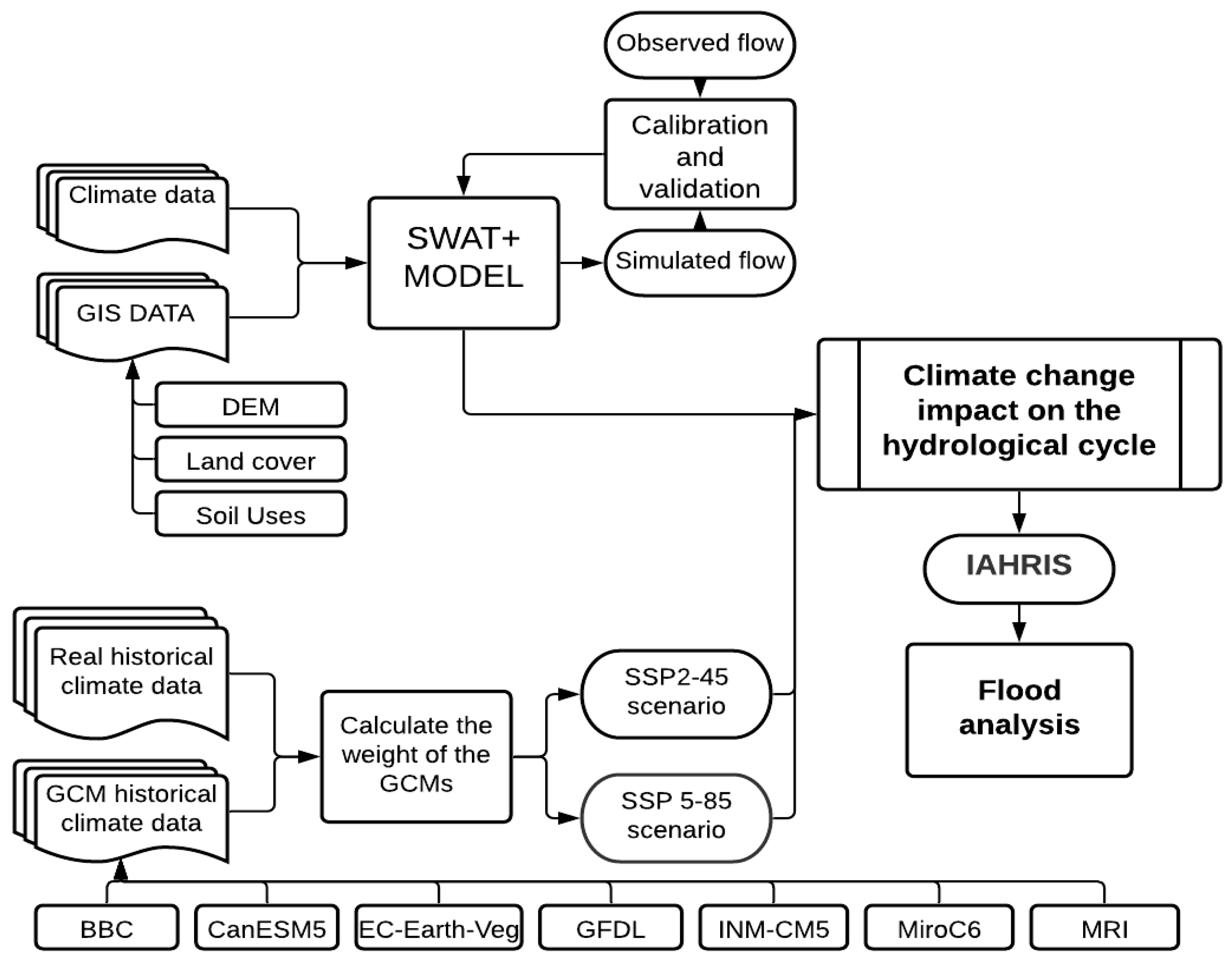
First, a SWAT+ model was developed, then calibrated and validated with observed streamflow and SWE satellite data. In addition, seven global climate models (GCMs) were weighted using real historical climate data as the reference. The future data were used under two climate change scenarios to simulate the water cycle of Lake Erken during a short-term period, a medium-term period and a long-term period. Finally, various parameters related to floods were calculated with Indicators of Hydrological Alteration in Rivers (IAHRIS) [
40]. The aim of this step was to compare the historical floods in Lake Erken with the projected floods that would be altered because of the climate change effects. The methodology of this article is represented in
Figure 1.
2.2. Description of the Study Area
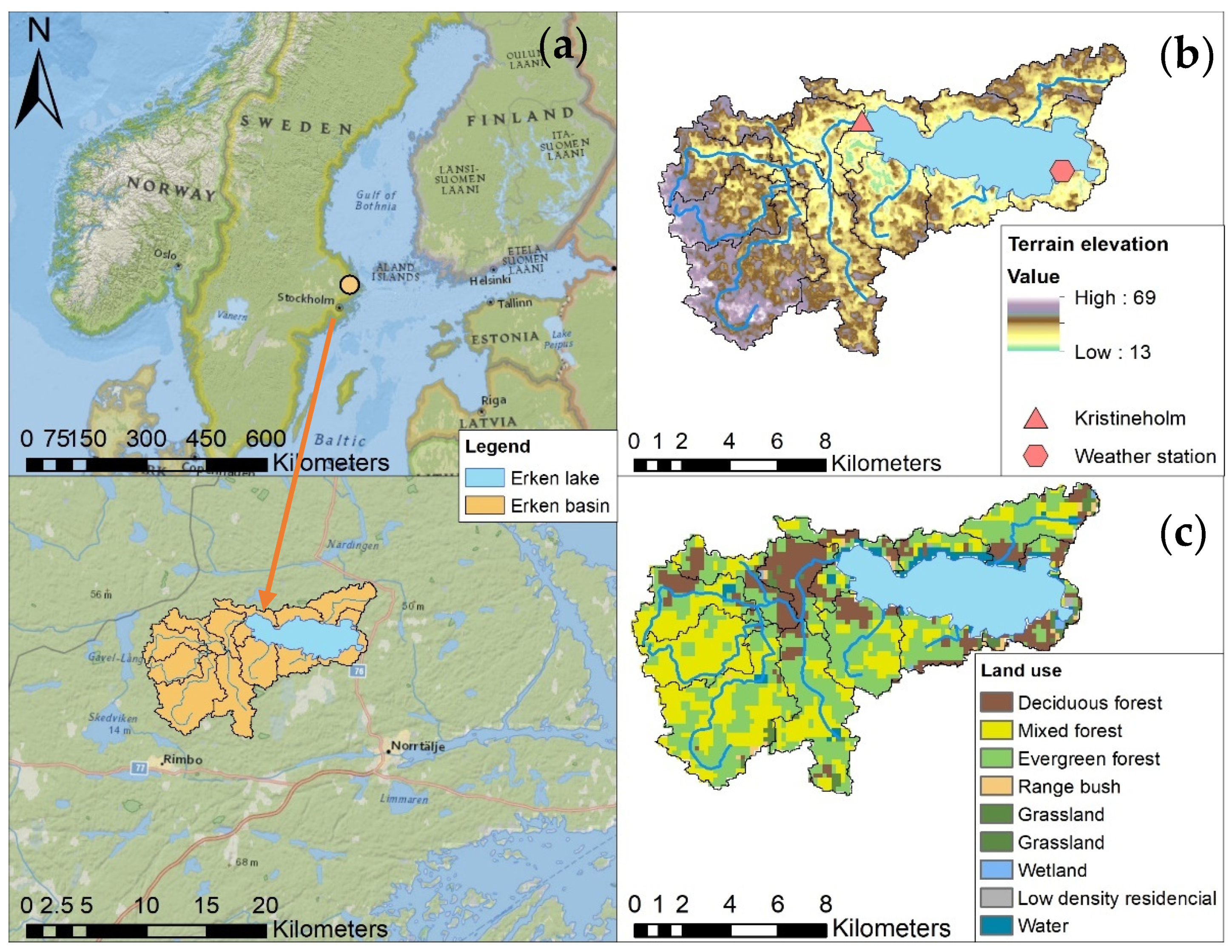
Lake Erken is located in the eastern part of Sweden (59°50′37″ N, 18°35′38″ E) at an altitude of 10 m above sea level (
Figure 2). The surface area of the lake is approximately 24 km
2. It is a shallow lake; the mean depth is around 9 m, and the deepest point is 21 m underwater. The lake has a residence time of 7.4 years. It can be described as a moderately eutrophic lake with an intermediate level of productivity. Its surface is usually ice-covered during winter, whereas during the summer, the water is stratified [
41,
42]. Both of these phenomena have been largely studied in Lake Erken [
43,
44,
45].
The Erken basin is oriented toward the east and does not present significant slopes. It is a relatively small drainage basin (141 km
2) that is covered by forest, without any significant anthropic activity [
46]. In the basin, there are exclusive areas of both deciduous forest and evergreen forest; in most of the basin, both types of vegetation share the space, forming a mixed forest that dominates the watershed (
Figure 2c). This forest plays a vital role in the water cycle. Forests regulate processes such as evapotranspiration, runoff, and water retention in forested basins [
47,
48,
49,
50,
51]. The main large water inflow point to the lake is Kristineholm (
Figure 2b). This input is where the water discharge for calibration and validation is measured.
In the south of Sweden, the climate is humid and continental, with a warm summer (17.3 °C average in July and August) and a weak winter—despite the country’s high latitude. The length of daylight varies from 18 h in June to 6 h in December. According to the historical data used in this study for 1990–2014, in the Erken basin the average temperature in July and August was 17.3 °C and in February it was −4 °C. Precipitation does not change much during the year but is slightly higher during autumn; the annual average is 519 mm. Precipitation in the form of snowfall occurs between December and March, and the basin is covered by snow for 75 to 100 days a year.
2.3. SWAT+ Model
The Soil and Water Assessment Tool (SWAT) [
29] software provides a hydrological model that is used worldwide. It has been successfully used in a range of scenarios with different climatic conditions, land management practices, and temporal and spatial scales. During the last 20 years, SWAT has been implemented periodically to meet the diverse requirements of the scientific community around the world. However, the current framework has reached the limit of its potential development. The most recent version, SWAT+, improves the runoff routing capabilities while preserving the model’s computational efficiency and ease of use [
28].
Water dynamics are represented by fluctuations in the hydrologic response units (HRUs) in both the SWAT and SWAT+ models. Each HRU is a unique combination of land-use, slope, soil, and management activities, which are connected by a geographic information system (GIS) interface. Using this GIS interface, in both models, the modelled basin is divided into various sub-basins, which are further sub-divided into HRUs [
52]. The concept of water balance, represented by Equation (1), is applied in the model as the watershed’s primary driver of all hydrology.
where
SWt and
SWo represent the final and initial soil water content (mm/day);
Vi represents the precipitation (mm/day);
Qi represents the surface runoff (mm/day);
Ei represents the evapotranspiration (mm/day);
Pi represents the percolation (mm/day);
QRi represents the return flow (mm/day); and ∆
t represents the time interval (day). The i term refers to the index.
Despite using the same equations, in SWAT+ the elements of the watershed—such as aquifers, land-use units, HRUs, ponds, and reservoirs—are defined as spatial objects. This feature enhances the flexibility of the configuration and discretisation of the basin compared with the earlier SWAT [
28].
2.4. Model Setup
The use of a hydrological model with SWAT+ requires specific geographical information about the area of interest. The data required include a digital elevation map (DEM), a land cover map, and a soil map. The model also requires meteorological input data. For this study, the DEM was obtained from the Shuttle Radar Topography Mission (SRTM). The SRTM uses a single-pass space-borne interferometric SAR system, which operates in both the C-band (5.6-cm) and the X-band (3-cm) frequencies to collect data about the earth’s surface elevation [
53]. The land cover map was obtained from Glob Cover 2015, which provides a 300-m resolution [
54]. The soil data were gathered from the Food and Agriculture Organisation of the United Nations’ Harmonised World Soil Date. This collection contains information for 16,000 map units with two soil layers, namely 0–30 and 30–100 cm deep [
55].
For the meteorological input data, daily precipitation and temperature data were obtained from the Erken Laboratory meteorological station (59°51′30.7080″ N, 18°24′17.5536″ E), situated on the Malma islet (
Figure 2b). This station provides automated measurements daily temperature and precipitation data and other information. The Hargreaves method was used to determine potential evapotranspiration [
56]; this method requires only the precipitation and temperature data. According to Oudin et al. [
57], hydrological models that employ parsimonious temperature-based methods perform similarly to models that use more data-demanding methods.
The calibration and validation of the simulated streamflow required discharge data. The discharge data available has been measured daily at Kristineholm, the largest input of Lake Erken, since mid-2006. In this study, the SWE was also calibrated. The SWE data from the Copernicus Global Land Service were used. It offers a 0.05° spatial resolution, calculated by integrating passive microwave radiometer brightness temperature readings from the Special Sensor Microwave Imager/Sounder with synoptic weather station network snow-depth data [
58].
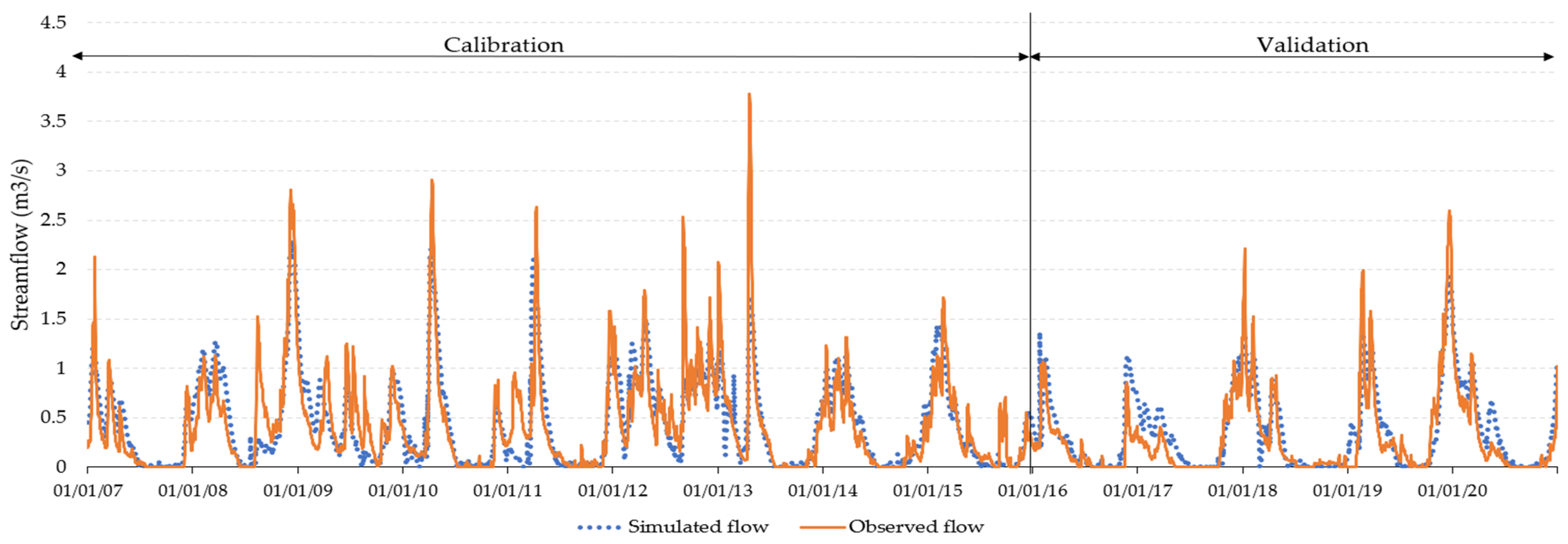
2.5. Calibration and Validation of the SWAT Model
To locate the most influential parameters for the streamflow, we performed a sensitivity analysis. Then, the sensitive parameters were adjusted with a daily automatic calibration for the 2007–2015 period. Both analyses were performed in Toolbox [
59], a free software designed to perform SWAT+ model sensitivity analysis, calibrations, and more. Afterwards, we used the 2016–2020 daily data to validate the SWAT+ model.
For the sensitivity analysis, Toolbox uses the Sobol method [
60]. Within an ensemble, it divides the overall output variance into the variation produced by each parameter. For automatic calibration, Toolbox uses a dynamically dimensioned search (DDS) [
60]. The Nash–Sutcliffe efficiency coefficient was applied as the target function in this investigation. The goodness of fit was determined using Moriasi’s four recommended statistics. In addition, for both calibration and validation, the performance was evaluated using Moriasi’s four recommended statistics [
61]. These are the coefficient of determination (R
2) (Equation (2)), the Nas–Sutcliffe efficiency (NSE) (Equation (3)), the standard deviation of measured data (RSR) (Equation (4)), and the per cent bias (PBIAS) (Equation (5)). The criteria proposed by Moriasi [
61] were applied. Both calibration and validation have been performed on a daily scale.
In Equations (2)–(5), the observed and simulated waterflow data are and ; the average observed and simulated water flow values are and and n refers to the total dataset.
To enhance the model, we performed a manual calibration of the SWE with the snow-related parameters. Since Toolbox does not allow for calibrating the SWE, we performed the calibration manually in SWAT+ Editor, which is a tool for editing, running, and saving changes to a SWAT model. Then, we validated each test in a spreadsheet by applying Equations (2)–(5) to the SWE.
2.6. Global Climate Models and Climate Change Scenarios
To make predictions for the Erken watershed, future climate models that simulate the temperature and precipitation in the coming years are required [
62]. Historical data from seven GCMs were downloaded from the Coupled Model Intercomparison Project (CIMP6) website (
https://esgf-node.llnl.gov/search/cmip6/, accessed on 26 November 2021) [
33]. The downloaded data were compared with the real historical data for precipitation and temperature in the Erken watershed. Based on the analysis of McSweeney et al. [
63], seven GCMs whose performance for Europe had been identified as satisfactory were selected: BBC, CanESM5, EC-Earth-Veg, GFDL, INM-CM5, MiroC6, and MRI. These seven GCMs were compared and assessed in this study. We used the methodology proposed by Pulido-Velazquez et al. [
55]. The Id indicator (Equation (6)) was calculated by summing the increases in the mean and variance of the control series over the historical series for the period 1985–2014, as follows:
where subscript
I is a subindex for a particular GCM, V1 is the rainfall variable, V2 is the temperature variable, S1 is the mean monthly value, S2 is the monthly standard deviation, and superscript
j is the number of months in a year. This indicator allows a ranking of GCMs to be established in terms of goodness of fit to the observed time series, so that an ensemble of predictions can be proposed, which gives more weight to the best scoring (lower Id index values). Then, the total Id indicator was rescaled by defining the Id* index, so that the sum of the values obtained for all models is equal to 1. Finally, the Ib indices were obtained, which are the complementary values of the Id* indicator, i.e., (1-Id*), rescaled to 1. These Ib indicators were used as weights applied to the series obtained with each model to create an ensemble of predictions.
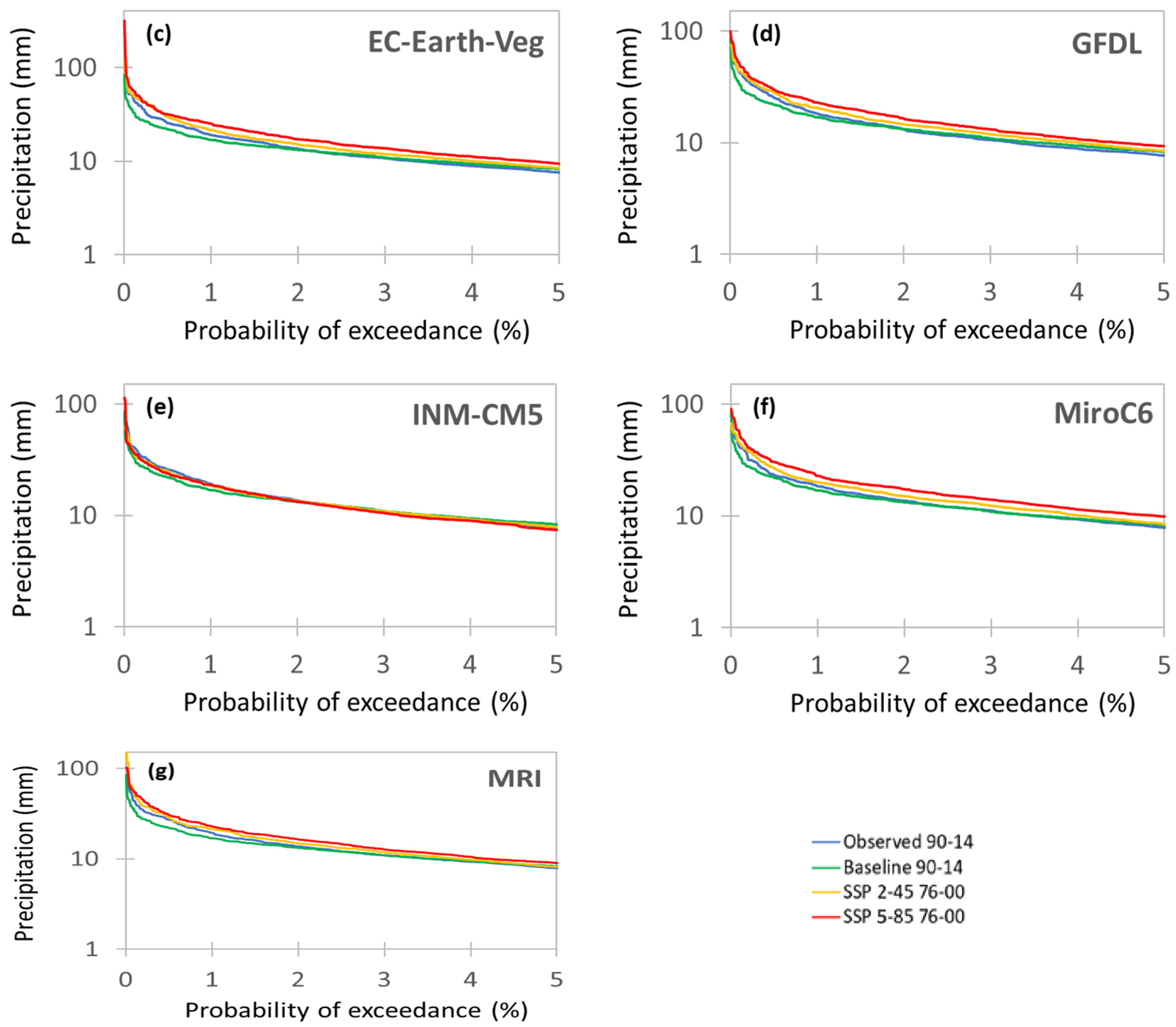
The historical data of each GCM were bias-corrected using the five statistical transformations available in the “qmap” package for R software. These were the robust empirical quantiles (RQUANT), distribution derived transformations (DIST), empirical quantiles (QUANT), parametric transformations (PTF), and smoothing spline (SSPLIN) [
64]. These methods try to align the distribution of simulated data with that of observed climate data and are commonly used in hydrological and climatic studies [
65,
66,
67].
The performance of the various methods was measured using the mean absolute error (MAE) between the observed and corrected data. This procedure is recommended by Gudmundsson et al. [
64]. The method that best fitted the observed historical data was selected for the correction of future climate change scenarios.
Lastly, the climate projection was analysed under two different shared socioeconomic pathway (SSP) scenarios [
68]. These were the SSP 2-45 and the SSP 5-85 scenarios. In the SSP 2, global emissions are predicted to follow current patterns. This implies significant obstacles for reduction and adaptation, but neither is particularly severe. On the other hand, the SSP 5 illustrates a scenario in which economic development takes precedence over environmental impacts. As a result, the challenges posed by climate change are difficult to meet [
69]. The SSP 2-45 and SSP 5-85 are, respectively, the equivalents of the RCP4.5 and RCP8.5 of the CMIP 5, updated with socioeconomic reasons [
70]. These two scenarios have been widely used in climate change studies because they allow a comparison between a more positive outlook (SSP 2-45) in which greenhouse gas emissions are intermediate and the effects of climate change are not as severe, and a more extreme outlook (SSP5-85) in which the challenges of climate change are greater.
2.7. IAHRIS Software
Indicators of Hydrologic Alteration (IHA) are commonly used to compare the variations in hydrological regimes between a base scenario and an altered scenario [
71]. IAHRIS is a software program created by the Centre for Public Works Studies and Experimentation (CEDEX) [
40]. It calculates various hydrological parameters of the flow and uses them to calculate various IHA. IAHRIS is particularly suited for evaluating flood events, since the indicators are divided into ordinary values, maximum extreme values (floods), and minimum extreme values (droughts). In addition, there are recent examples of previous studies that use IAHRIS and SWAT with satisfactory results [
72,
73]. In this work, IAHRIS was used to compare historical floods in Lake Erken with the projected floods that were altered in the future because of climate change effects. To study extreme peak flow events (floods) IAHRIS offers 8 parameters (Qc, Ql, Qconnec, Q5%, CV (Qc), CV (Q5%), consecutive days of flooding and flood days per month), which are described as follows. To analyse the magnitude and frequency of the floods, we used:
- -
Qc: the mean of the maximum annual daily flow.
- -
Ql: bed generation flow; this parameter represents the flow that performs most of the work of material relocation and is responsible for the geomorphology of the channel.
- -
Qconnec: the maximum flow that ensures the river channel–floodplain connection is represented by the connectivity flow.
- -
Q5%: this parameter is the flow corresponding to the average flow curve classified at the 5% exceedance percentile.
To analyse the variability of the floods, we used:
- -
CV (Qc): coefficient of variation of the series of maximum annual daily flow rates.
- -
CV (Q5%): coefficient of variation of the series of usual floods.
To study the duration of the floods, we used the maximum number of consecutive days with an average daily flow rate greater than the Q5%. Lastly, IAHRIS offers the flood days per month to analyse the seasonality of the floods.
More information about these parameters appears in the IAHRIS methodological reference manual [
74].


 ,
, 


