
Response of Spatio-Temporal Differentiation Characteristics of Habitat Quality to Land Surface Temperature in a Fast Urbanized City


Abstract
:1. Introduction
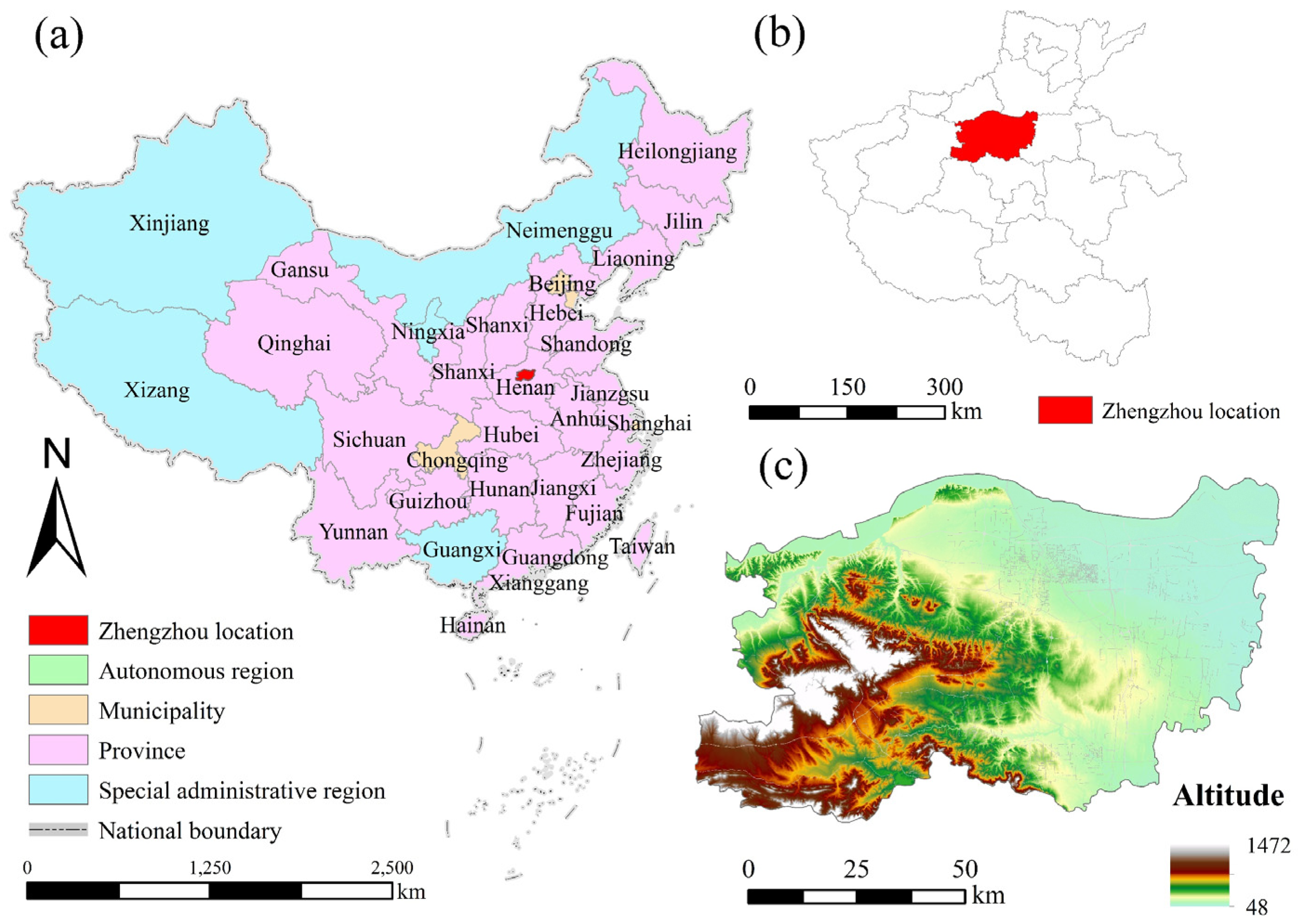
2. Study Area
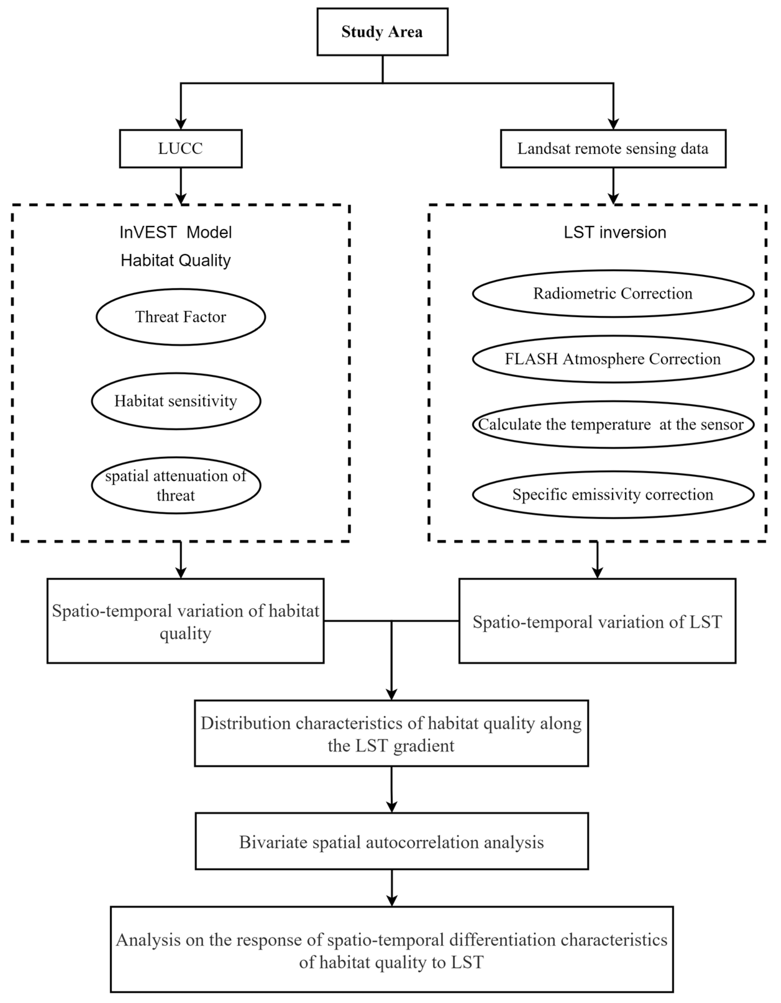
3. Data Sources and Methods
3.1. Data Used
3.2. Habitat Quality Calculation
3.3. LST Inversion Calculation
3.4. Bivariate Moran’s I Calculation
4. Results
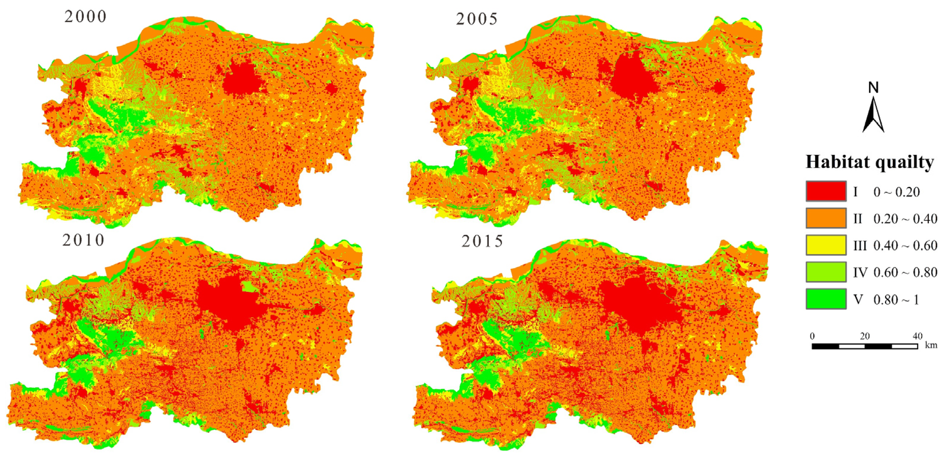
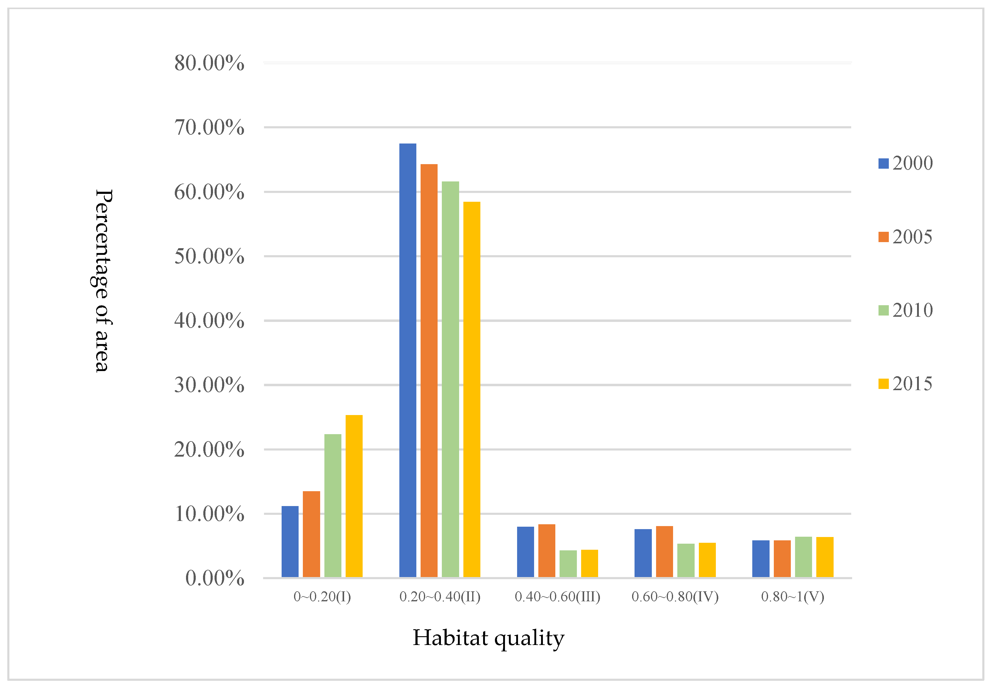
4.1. Spatio-Temporal Variation of Habitat Quality
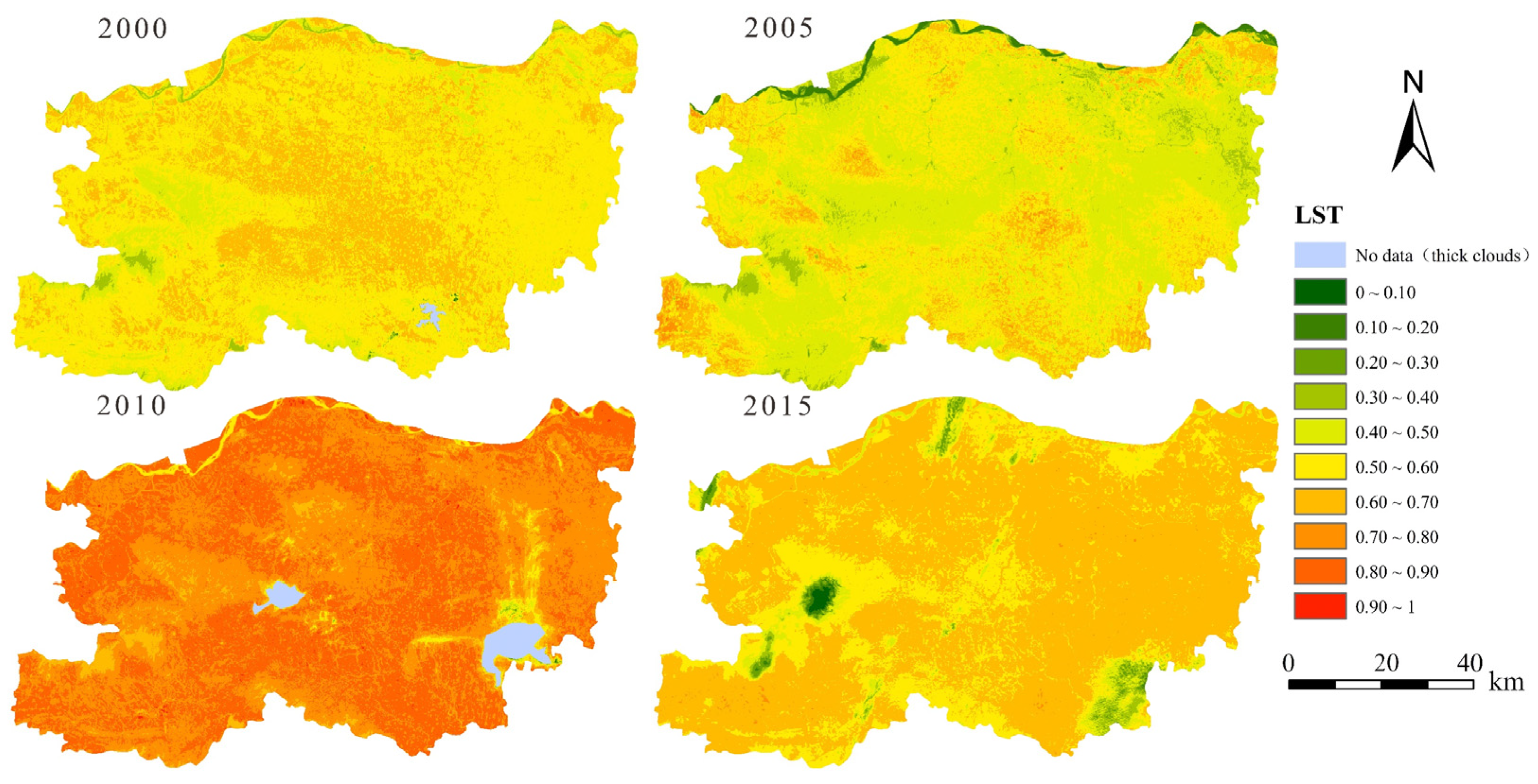
4.2. Spatio-Temporal Variation of LST
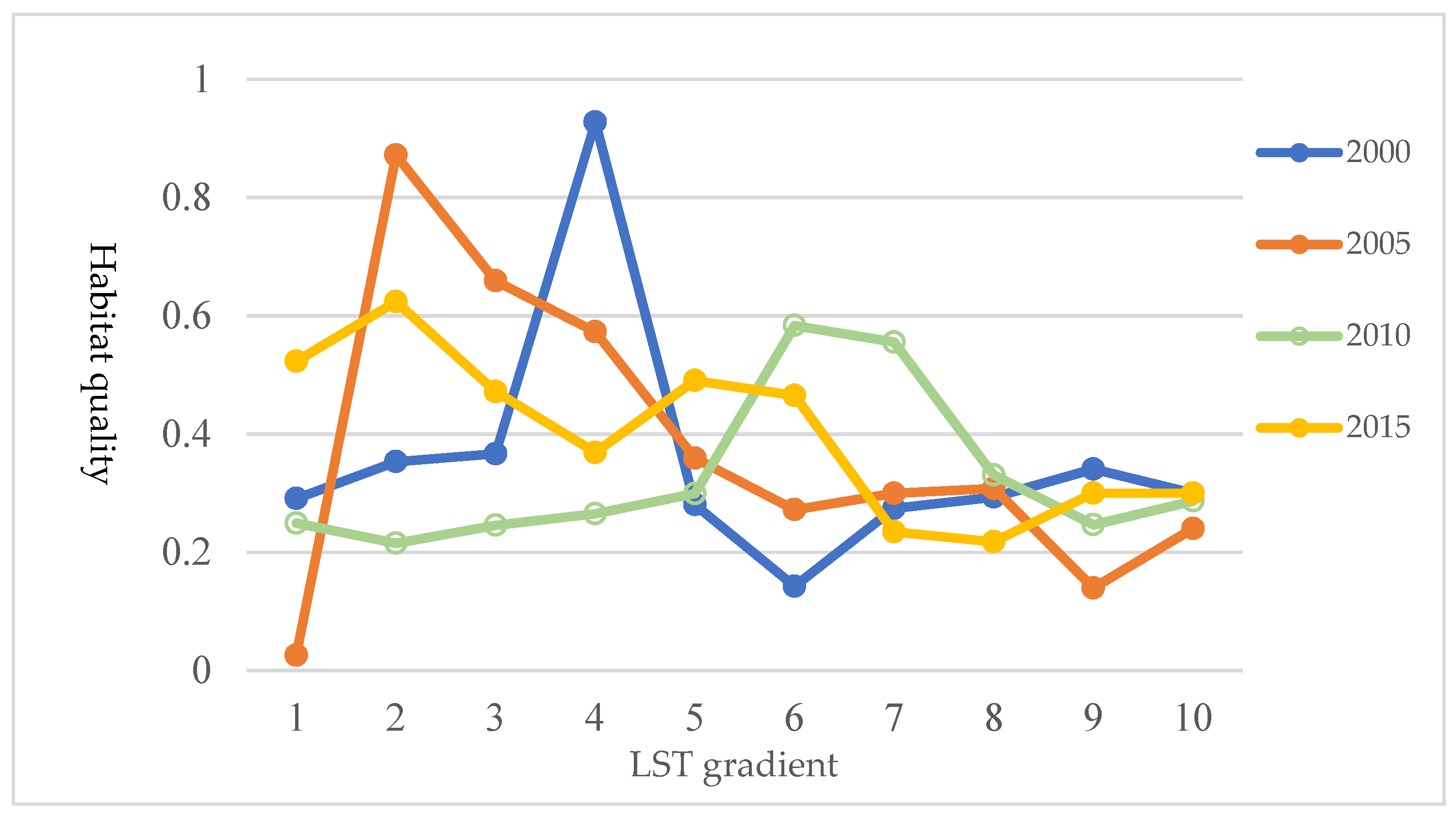
4.3. The Distribution of Habitat Quality along LST Gradients
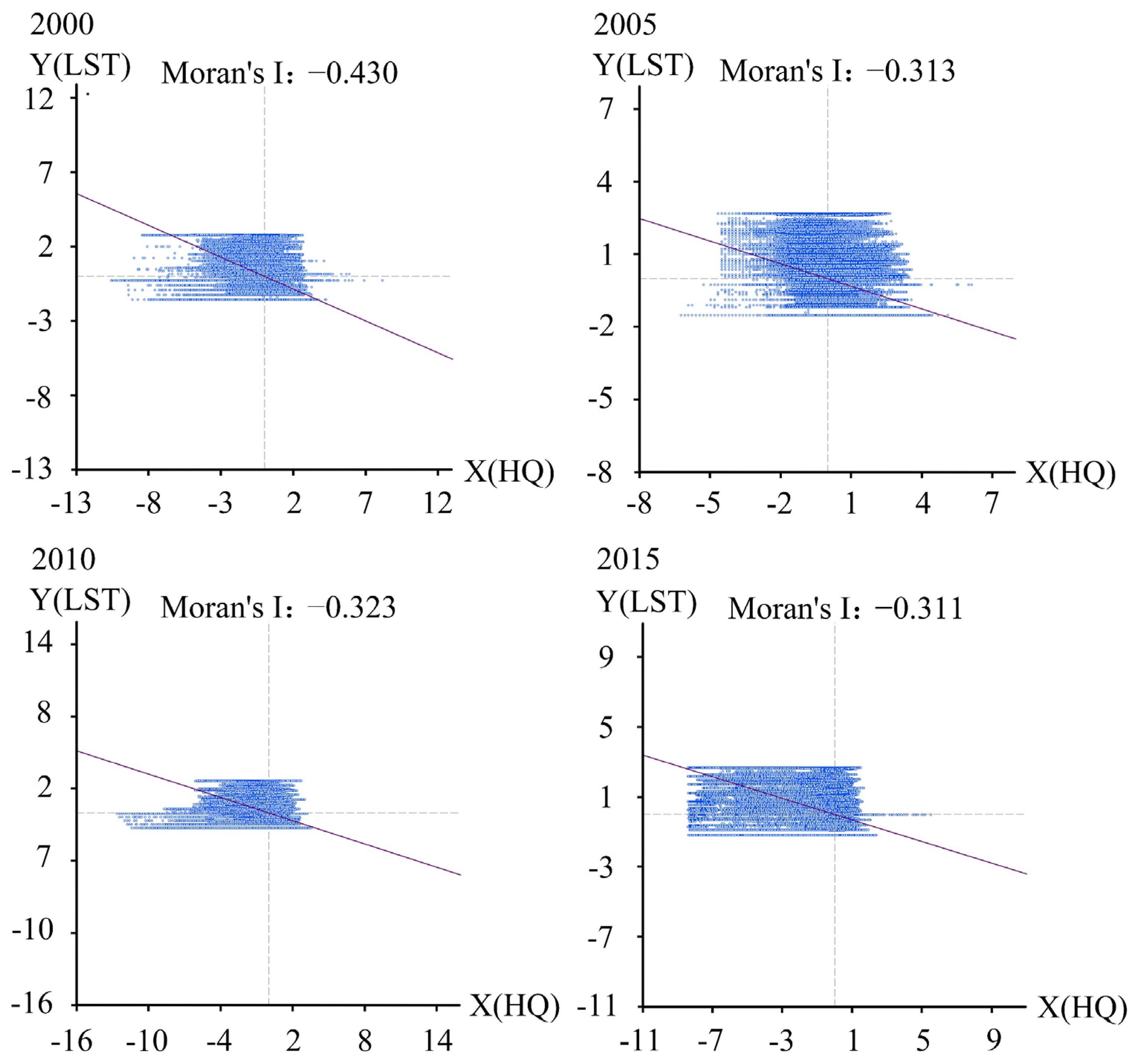
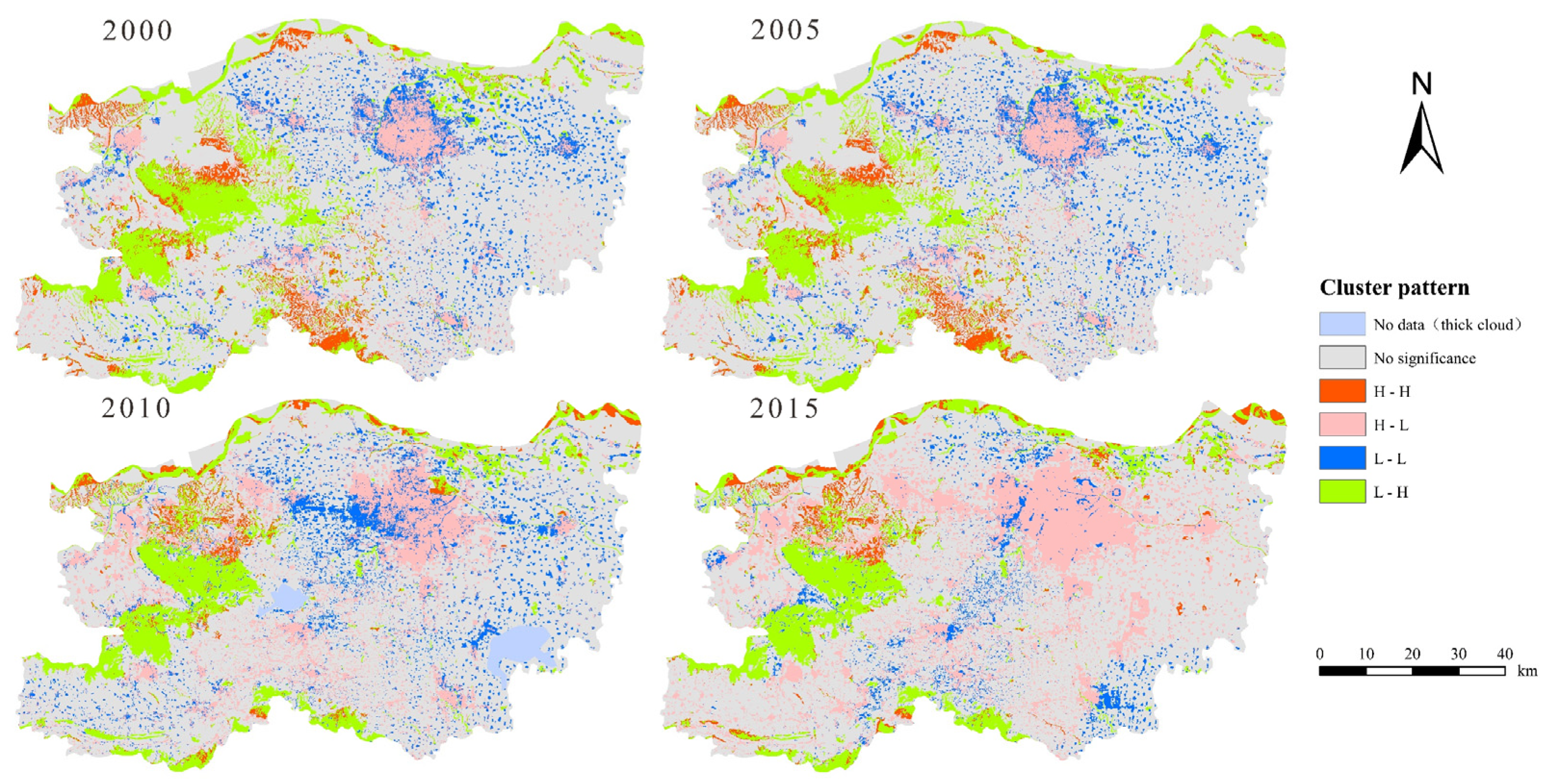
4.4. Bivariate Spatial Autocorrelation Analysis
5. Discussion
6. Conclusions
Author Contributions
Funding
Data Availability Statement
Acknowledgments
Conflicts of Interest
References
- Di Febbraro, M.; Sallustio, L.; Vizzarri, M.; De Rosa, D.; De Lisio, L.; Loy, A.; Eichelberger, B.A.; Marchetti, M. Expert-Based and Correlative Models to Map Habitat Quality: Which Gives Better Support to Conservation Planning? Glob. Ecol. Conserv. 2018, 16, e00513. [Google Scholar] [CrossRef]
- Mori, A.S.; Dee, L.E.; Gonzalez, A.; Ohashi, H.; Isbell, F. Biodiversity–Productivity Relationships Are Key to Nature-Based Climate Solutions. Nat. Clim. Chang. 2021, 11, 543–550. [Google Scholar] [CrossRef]
- Lavergne, S.; Mouquet, N.; Thuiller, W.; Ronce, O. Biodiversity and Climate Change: Integrating Evolutionary and Ecological Responses of Species and Communities. Annu. Rev. Ecol. Evol. Syst. 2010, 41, 321–350. [Google Scholar] [CrossRef] [Green Version]
- Hemanth Kumar, N.K.; Murali, M.; Girish, H.V.; Chandrashekar, S.; Amruthesh, K.N.; Sreenivasa, M.Y.; Jagannath, S. 2—Impact of Climate Change on Biodiversity and Shift in Major Biomes. In Global Climate Change; Singh, S., Singh, P., Rangabhashiyam, S., Srivastava, K.K., Eds.; Elsevier: Amsterdam, The Netherlands, 2021; pp. 33–44. ISBN 978-0-12-822928-6. [Google Scholar]
- Nath, S.; Shyanti, R.K.; Nath, Y. 4—Influence of Anthropocene Climate Change on Biodiversity Loss in Different Ecosystems. In Global Climate Change; Singh, S., Singh, P., Rangabhashiyam, S., Srivastava, K.K., Eds.; Elsevier: Amsterdam, The Netherlands, 2021; pp. 63–78. ISBN 978-0-12-822928-6. [Google Scholar]
- Li, Z.-L.; Tang, B.-H.; Wu, H.; Ren, H.; Yan, G.; Wan, Z.; Trigo, I.F.; Sobrino, J.A. Satellite-Derived Land Surface Temperature: Current Status and Perspectives. Remote Sens. Environ. 2013, 131, 14–37. [Google Scholar] [CrossRef] [Green Version]
- Gillespie, A.; Rokugawa, S.; Matsunaga, T.; Cothern, J.S.; Hook, S.; Kahle, A.B. A Temperature and Emissivity Separation Algorithm for Advanced Spaceborne Thermal Emission and Reflection Radiometer (ASTER) Images. IEEE Trans. Geosci. Remote Sens. 1998, 36, 1113–1126. [Google Scholar] [CrossRef]
- Zhou, D.; Xiao, J.; Bonafoni, S.; Berger, C.; Deilami, K.; Zhou, Y.; Frolking, S.; Yao, R.; Qiao, Z.; Sobrino, J.A. Satellite Remote Sensing of Surface Urban Heat Islands: Progress, Challenges, and Perspectives. Remote Sens. 2019, 11, 48. [Google Scholar] [CrossRef] [Green Version]
- Friedl, M.A. Forward and Inverse Modeling of Land Surface Energy Balance Using Surface Temperature Measurements. Remote Sens. Environ. 2002, 79, 344–354. [Google Scholar] [CrossRef]
- Qi, Y.; Lian, X.; Wang, H.; Zhang, J.; Yang, R. Dynamic Mechanism between Human Activities and Ecosystem Services: A Case Study of Qinghai Lake Watershed, China. Ecol. Indic. 2020, 117, 106528. [Google Scholar] [CrossRef]
- Rushing, C.S.; Royle, J.A.; Ziolkowski, D.J.; Pardieck, K.L. Migratory Behavior and Winter Geography Drive Differential Range Shifts of Eastern Birds in Response to Recent Climate Change. Proc. Natl. Acad. Sci. USA 2020, 117, 12897–12903. [Google Scholar] [CrossRef] [PubMed]
- Johnson, M.D. Measuring Habitat Quality: A Review. Condor 2007, 109, 489–504. [Google Scholar] [CrossRef]
- Lin, Y.-P.; Lin, W.-C.; Wang, Y.-C.; Lien, W.-Y.; Huang, T.; Hsu, C.-C.; Schmeller, D.S.; Crossman, N.D. Systematically Designating Conservation Areas for Protecting Habitat Quality and Multiple Ecosystem Services. Environ. Model. Softw. 2017, 90, 126–146. [Google Scholar] [CrossRef]
- Tallis, H.; Lubchenco, J. Working Together: A Call for Inclusive Conservation. Nature 2014, 515, 27–28. [Google Scholar] [CrossRef] [PubMed] [Green Version]
- Jill, B. Planetary Health: Protecting Nature to Protect Ourselves. Samuel Myers and Howard Frumkin (Eds). Int. J. Epidemiol. 2021, 50, 697–698. [Google Scholar] [CrossRef]
- Seto, K.C.; Guneralp, B.; Hutyra, L. Global Forecasts of Urban Expansion to 2030 and Direct Impacts on Biodiversity and Carbon Pools. Proc. Natl. Acad. Sci. USA 2012, 109, 16083–16088. [Google Scholar] [CrossRef] [Green Version]
- Kowarik, I. Novel Urban Ecosystems, Biodiversity, and Conservation. Environ. Pollut. 2011, 159, 1974–1983. [Google Scholar] [CrossRef] [PubMed]
- Feest, A.; Aldred, T.D.; Jedamzik, K. Biodiversity Quality: A Paradigm for Biodiversity. Ecol. Indic. 2010, 10, 1077–1082. [Google Scholar] [CrossRef] [Green Version]
- Magurran, A.E.; Baillie, S.R.; Buckland, S.T.; Dick, J.M.; Elston, D.A.; Scott, E.M.; Smith, R.I.; Somerfield, P.J.; Watt, A.D. Long-Term Datasets in Biodiversity Research and Monitoring: Assessing Change in Ecological Communities through Time. Trends Ecol. Evol. 2010, 25, 574–582. [Google Scholar] [CrossRef]
- Sherrouse, B.C.; Semmens, D.J.; Clement, J.M. An Application of Social Values for Ecosystem Services (SolVES) to Three National Forests in Colorado and Wyoming. Ecol. Indic. 2014, 36, 68–79. [Google Scholar] [CrossRef]
- Sharps, K.; Masante, D.; Thomas, A.; Jackson, B.; Redhead, J.; May, L.; Prosser, H.; Cosby, B.; Emmett, B.; Jones, L. Comparing Strengths and Weaknesses of Three Ecosystem Services Modelling Tools in a Diverse UK River Catchment. Sci. Total Environ. 2017, 584, 118–130. [Google Scholar] [CrossRef] [PubMed] [Green Version]
- Huang, Z.; Bai, Y.; Alatalo, J.M.; Yang, Z. Mapping Biodiversity Conservation Priorities for Protected Areas: A Case Study in Xishuangbanna Tropical Area, China. Biol. Conserv. 2020, 249, 108741. [Google Scholar] [CrossRef]
- Sohn, H.-J.; Kim, D.-H.; Kim, N.-Y.; Hong, J.-P.; Song, Y.-K. Evaluation indicators for the restoration of degraded urban ecosystems and the analysis of restoration performance. J. Korean Soc. Environ. Restor. Technol. 2019, 22, 97–114. [Google Scholar] [CrossRef]
- Kija, H.K.; Ogutu, J.O.; Mangewa, L.J.; Bukombe, J.; Verones, F.; Graae, B.J.; Kideghesho, J.R.; Said, M.Y.; Nzunda, E.F. Spatio-Temporal Changes in Wildlife Habitat Quality in the Greater Serengeti Ecosystem. Sustainability 2020, 12, 2440. [Google Scholar] [CrossRef] [Green Version]
- Yu, W.; Ji, R.; Han, X.; Chen, L.; Feng, R.; Wu, J.; Zhang, Y. Evaluation of the Biodiversity Conservation Function in Liaohe Delta Wetland, Northeastern China. J. Meteorol. Res. 2020, 34, 798–805. [Google Scholar] [CrossRef]
- Benez-Secanho, F.J.; Dwivedi, P. Analyzing the Provision of Ecosystem Services by Conservation Easements and Other Protected and Non-Protected Areas in the Upper Chattahoochee Watershed. Sci. Total Environ. 2020, 717, 137218. [Google Scholar] [CrossRef]
- Rimal, B.; Sharma, R.; Kunwar, R.; Keshtkar, H.; Stork, N.E.; Rijal, S.; Rahman, S.A.; Baral, H. Effects of Land Use and Land Cover Change on Ecosystem Services in the Koshi River Basin, Eastern Nepal. Ecosyst. Serv. 2019, 38, 100963. [Google Scholar] [CrossRef]
- Dai, L.; Li, S.; Lewis, B.J.; Wu, J.; Yu, D.; Zhou, W.; Zhou, L.; Wu, S. The Influence of Land Use Change on the Spatial–Temporal Variability of Habitat Quality between 1990 and 2010 in Northeast China. J. For. Res. 2019, 30, 2227–2236. [Google Scholar] [CrossRef]
- Zhang, T.; Gao, Y.; Li, C.; Xie, Z.; Chang, Y.; Zhang, B. How Human Activity Has Changed the Regional Habitat Quality in an Eco-Economic Zone: Evidence from Poyang Lake Eco-Economic Zone, China. Int. J. Environ. Res. Public Health 2020, 17, 6253. [Google Scholar] [CrossRef] [PubMed]
- Long, H.; Liu, Y.; Hou, X.; Li, T.; Li, Y. Effects of Land Use Transitions Due to Rapid Urbanization on Ecosystem Services: Implications for Urban Planning in the New Developing Area of China. Habitat Int. 2014, 44, 536–544. [Google Scholar] [CrossRef]
- Zhu, C.; Zhang, X.; Zhou, M.; He, S.; Gan, M.; Yang, L.; Wang, K. Impacts of Urbanization and Landscape Pattern on Habitat Quality Using OLS and GWR Models in Hangzhou, China. Ecol. Indic. 2020, 117, 106654. [Google Scholar] [CrossRef]
- Yohannes, H.; Soromessa, T.; Argaw, M.; Dewan, A. Spatio-Temporal Changes in Habitat Quality and Linkage with Landscape Characteristics in the Beressa Watershed, Blue Nile Basin of Ethiopian Highlands. J. Environ. Manag. 2021, 281, 111885. [Google Scholar] [CrossRef] [PubMed]
- Wang, H.; Tang, L.; Qiu, Q.; Chen, H. Assessing the Impacts of Urban Expansion on Habitat Quality by Combining the Concepts of Land Use, Landscape, and Habitat in Two Urban Agglomerations in China. Sustainability 2020, 12, 4346. [Google Scholar] [CrossRef]
- Song, S.; Liu, Z.; He, C.; Lu, W. Evaluating the Effects of Urban Expansion on Natural Habitat Quality by Coupling Localized Shared Socioeconomic Pathways and the Land Use Scenario Dynamics-Urban Model. Ecol. Indic. 2020, 112, 106071. [Google Scholar] [CrossRef]
- Nematollahi, S.; Fakheran, S.; Kienast, F.; Jafari, A. Application of InVEST Habitat Quality Module in Spatially Vulnerability Assessment of Natural Habitats (Case Study: Chaharmahal and Bakhtiari Province, Iran). Environ. Monit. Assess. 2020, 192, 487. [Google Scholar] [CrossRef] [PubMed]
- Zhang, H.; Zhang, C.; Hu, T.; Zhang, M.; Ren, X.; Hou, L. Exploration of Roadway Factors and Habitat Quality Using InVEST. Transp. Res. Part D Transp. Environ. 2020, 87, 102551. [Google Scholar] [CrossRef]
- Zhang, H.B.; Liu, Y.Q.; Xu, Y.; Han, S.; Wang, J. Impacts of Spartina Alterniflora Expansion on Landscape Pattern and Habitat Quality: A Case Study in Yancheng Coastal Wetland, China. Appl. Ecol. Environ. Res. 2020, 18, 4669–4683. [Google Scholar] [CrossRef]
- Liu, J.; Zhang, Z.; Xu, X.; Kuang, W.; Zhou, W.; Zhang, S.; Li, R.; Yan, C.; Yu, D.; Wu, S.; et al. Spatial Patterns and Driving Forces of Land Use Change in China during the Early 21st Century. J. Geogr. Sci. 2010, 20, 483–494. [Google Scholar] [CrossRef]
- Xu, X.; Liu, J.; Zhang, S.; Li, R.; Yan, C.; Wu, S. China multi period land use and land cover remote sensing monitoring data set (CNLUCC). Data Regist. Publ. Syst. Resour. Environ. Sci. Data Cent. Acad. Sci. 2018. [Google Scholar] [CrossRef]
- Nie, C.; Yang, J.; Huang, C. Assessing the Habitat Quality of Aquatic Environments in Urban Beijing. Procedia Environ. Sci. 2016, 36, 162–168. [Google Scholar] [CrossRef] [Green Version]
- Lee, D.J.; Jeon, S.W. Estimating Changes in Habitat Quality through Land-Use Predictions: Case Study of Roe Deer (Capreolus Pygargus Tianschanicus) in Jeju Island. Sustainability 2020, 12, 123. [Google Scholar] [CrossRef]
- Choudhary, A.; Deval, K.; Joshi, P.K. Study of Habitat Quality Assessment Using Geospatial Techniques in Keoladeo National Park, India. Environ. Sci. Pollut. Res. 2021, 28, 14105–14114. [Google Scholar] [CrossRef] [PubMed]
- Li, X.; Yu, X.; Wu, K.; Feng, Z.; Liu, Y.; Li, X. Land-Use Zoning Management to Protecting the Regional Key Ecosystem Services: A Case Study in the City Belt along the Chaobai River, China. Sci. Total Environ. 2020, 24, 143167. [Google Scholar] [CrossRef] [PubMed]
- Tomlinson, C.J.; Chapman, L.; Thornes, J.E.; Baker, C. Remote Sensing Land Surface Temperature for Meteorology and Climatology: A Review. Meteorol. Appl. 2011, 18, 296–306. [Google Scholar] [CrossRef] [Green Version]
- Sobrino, J.A.; Jiménez-Muñoz, J.C.; Paolini, L. Land Surface Temperature Retrieval from LANDSAT TM 5. Remote Sens. Environ. 2004, 90, 434–440. [Google Scholar] [CrossRef]
- Moran, P.A. Notes on Continuous Stochastic Phenomena. Biometrika 1950, 37, 17–23. [Google Scholar] [CrossRef] [PubMed]
- Anselin, L. Local Indicators of Spatial Association—LISA. Geogr. Anal. 2010, 27, 93–115. [Google Scholar] [CrossRef]
- Mills, G. Urban Climatology: History, Status and Prospects. Urban Clim. 2014, 10, 479–489. [Google Scholar] [CrossRef]
- Hua, L.; Zhang, X.; Nie, Q.; Sun, F.; Tang, L. The Impacts of the Expansion of Urban Impervious Surfaces on Urban Heat Islands in a Coastal City in China. Sustainability 2020, 12, 475. [Google Scholar] [CrossRef] [Green Version]
- Sturiale, L.; Scuderi, A. The Role of Green Infrastructures in Urban Planning for Climate Change Adaptation. Climate 2019, 7, 119. [Google Scholar] [CrossRef] [Green Version]
- Kato, M.; Yoshizaki, S.; Hashida, S.; Lee, K.; Suzuki, H. The Evaluation of Tree Species of Urban Greening in Japan for Increasing the Bio-Diversity in Urban Area. J. Jpn. Soc. Reveg. Technol. 2016, 42, 3–8. [Google Scholar] [CrossRef] [Green Version]
- Belaud, J.P.; Adoue, C.; Vialle, C.; Chorro, A.; Sablayrolles, C. A Circular Economy and Industrial Ecology Toolbox for Developing an Eco-Industrial Park: Perspectives from French Policy. Clean Technol. Environ. Policy 2019, 21, 967–985. [Google Scholar] [CrossRef] [Green Version]
- Kardooni, R.; Yusoff, S.B.; Kari, F.B.; Moeenizadeh, L. Public Opinion on Renewable Energy Technologies and Climate Change in Peninsular Malaysia. Renew. Energy 2018, 116, 659–668. [Google Scholar] [CrossRef]
- Qazi, A.; Hussain, F.; Rahim, N.A.B.D.; Hardaker, G.; Alghazzawi, D.; Shaban, K.; Haruna, K. Towards Sustainable Energy: A Systematic Review of Renewable Energy Sources, Technologies, and Public Opinions. IEEE Access 2019, 7, 63837–63851. [Google Scholar] [CrossRef]
- Firake, D.M.; Lytan, D.; Behere, G.T. Bio-Diversity and Seasonal Activity of Arthropod Fauna in Brassicaceous Crop Ecosystems of Meghalaya, North East India. Mol. Entomol. 2013, 3, 18–22. [Google Scholar] [CrossRef]
- Beninde, J.; Veith, M.; Hochkirch, A. Biodiversity in Cities Needs Space: A Meta-Analysis of Factors Determining Intra-Urban Biodiversity Variation. Ecol. Lett. 2015, 18, 581–592. [Google Scholar] [CrossRef]
- Krosby, M.; Tewksbury, J.; Haddad, N.M.; Hoekstra, J. Ecological Connectivity for a Changing Climate. Conserv. Biol. 2010, 24, 1686–1689. [Google Scholar] [CrossRef] [PubMed]
- Nor, A.N.M.; Corstanje, R.; Harris, J.A.; Grafius, D.R.; Siriwardena, G.M. Ecological Connectivity Networks in Rapidly Expanding Cities. Heliyon 2017, 3, e00325. [Google Scholar] [CrossRef] [PubMed] [Green Version]
- Antar, M.; Lyu, D.; Nazari, M.; Shah, A.; Zhou, X.; Smith, D.L. Biomass for a Sustainable Bioeconomy: An Overview of World Biomass Production and Utilization. Renew. Sustain. Energy Rev. 2021, 139, 110691. [Google Scholar] [CrossRef]
- Koukios, E.; Monteleone, M.; Carrondo, M.J.T.; Charalambous, A.; Girio, F.; Hernández, E.L.; Mannelli, S.; Parajó, J.C.; Polycarpou, P.; Zabaniotou, A. Targeting Sustainable Bioeconomy: A New Development Strategy for Southern European Countries. The Manifesto of the European Mezzogiorno. J. Clean. Prod. 2018, 172, 3931–3941. [Google Scholar] [CrossRef] [Green Version]


| Habitat Type | Habitat Suitability | Threat Factor | |||||
|---|---|---|---|---|---|---|---|
| Main Category | Subcategory | Paddy Field | Dry Land | Built-Up Land | Rural Residential Land | Other Construction Land | |
| Cultivated land | Paddy field | 0.4 | 0 | 1 | 0.5 | 0.3 | 0.4 |
| Dry land | 0.3 | 1 | 0 | 0.5 | 0.3 | 0.4 | |
| Forest | Woodland | 1 | 0.8 | 0.9 | 0.9 | 0.8 | 0.8 |
| Shrubwood | 0.7 | 0.4 | 0.5 | 0.6 | 0.4 | 0.5 | |
| Sparse woodland | 0.6 | 0.8 | 0.9 | 0.5 | 0.7 | 0.8 | |
| Other woodland | 0.5 | 0.9 | 1 | 0.5 | 0.7 | 0.8 | |
| Grassland | High coverage grassland | 0.7 | 0.4 | 0.5 | 0.8 | 0.45 | 0.7 |
| Medium coverage grassland | 0.5 | 0.5 | 0.6 | 0.7 | 0.5 | 0.6 | |
| Low coverage grassland | 0.3 | 0.7 | 0.9 | 0.6 | 0.55 | 0.5 | |
| Water | River and canal | 1 | 0.7 | 0.5 | 0.7 | 0.6 | 0.6 |
| Lake | 0.9 | 0.7 | 0.5 | 0.7 | 0.6 | 0.6 | |
| Reservoir and pond | 0.8 | 0.8 | 0.4 | 0.8 | 0.7 | 0.7 | |
| Bottomland | 0.6 | 0 | 0 | 0.9 | 0.8 | 0.7 | |
| Construction land | Built-up land | 0 | 0 | 0 | 0 | 0 | 0 |
| Rural residential land | 0 | 0 | 0 | 0 | 0 | 0 | |
| Other construction land | 0 | 0 | 0 | 0 | 0 | 0 | |
| Unused land | Sandy land | 0.1 | 0.1 | 0.1 | 0.2 | 0.1 | 0.1 |
| Saline-alkali land | 0.1 | 0.1 | 0.1 | 0.2 | 0.1 | 0.1 | |
| Marshland | 0.6 | 0.5 | 0.6 | 0.8 | 0.6 | 0.5 | |
| Bare soil land | 0 | 0 | 0 | 0 | 0 | 0 | |
| Bare rock land | 0 | 0 | 0 | 0 | 0 | 0 | |
| Threat Source | Relative Weight | Maximum Influence Distance (km) | Spatial Attenuation Function |
|---|---|---|---|
| Paddy field | 0.4 | 4 | Exponential |
| Dry land | 0.3 | 4 | Exponential |
| Built-up land | 1 | 8 | Exponential |
| Rural residential land | 0.6 | 6 | Exponential |
| Other construction land | 0.8 | 5 | Exponential |
Publisher’s Note: MDPI stays neutral with regard to jurisdictional claims in published maps and institutional affiliations. |
© 2021 by the authors. Licensee MDPI, Basel, Switzerland. This article is an open access article distributed under the terms and conditions of the Creative Commons Attribution (CC BY) license (https://creativecommons.org/licenses/by/4.0/).
Share and Cite
Hu, Y.; Xu, E.; Kim, G.; Liu, C.; Tian, G. Response of Spatio-Temporal Differentiation Characteristics of Habitat Quality to Land Surface Temperature in a Fast Urbanized City. Forests 2021, 12, 1668. https://doi.org/10.3390/f12121668
Hu Y, Xu E, Kim G, Liu C, Tian G. Response of Spatio-Temporal Differentiation Characteristics of Habitat Quality to Land Surface Temperature in a Fast Urbanized City. Forests. 2021; 12(12):1668. https://doi.org/10.3390/f12121668
Chicago/Turabian StyleHu, Yongge, Enkai Xu, Gunwoo Kim, Chang Liu, and Guohang Tian. 2021. "Response of Spatio-Temporal Differentiation Characteristics of Habitat Quality to Land Surface Temperature in a Fast Urbanized City" Forests 12, no. 12: 1668. https://doi.org/10.3390/f12121668
APA StyleHu, Y., Xu, E., Kim, G., Liu, C., & Tian, G. (2021). Response of Spatio-Temporal Differentiation Characteristics of Habitat Quality to Land Surface Temperature in a Fast Urbanized City. Forests, 12(12), 1668. https://doi.org/10.3390/f12121668