
A Compromise Programming Application to Support Forest Industrial Plantation Decision-Makers


Abstract
1. Introduction
2. Material and Methods
2.1. Case Study
2.2. Brief Description of Romero®
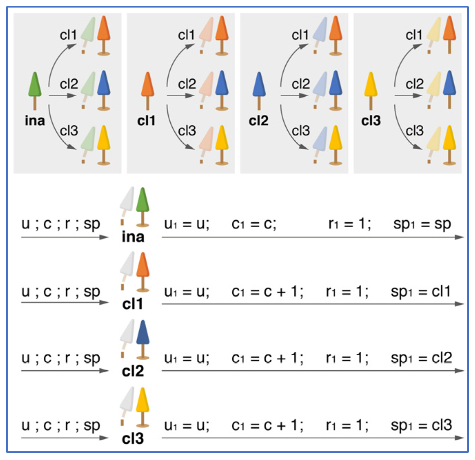
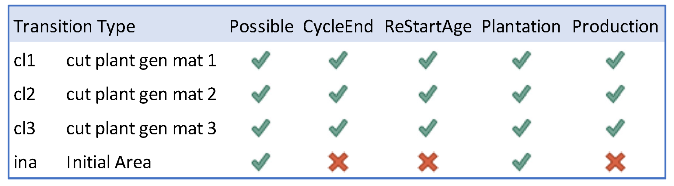
2.2.1. Forest Harvest Schedule Formulation
2.2.2. Multicriteria Concepts Embedded in Romero®
- (a)
- Attributes. These values are calculated independently from any stakeholder’s choice. In our case study, a “Production” accounting variable could be written using the expression, which is the total production within the horizon. It is called xTotalProd.
- (b)
- Objectives. They are all available to be selected by the user. If the user selects the attribute xTotalProd to form a maximization objective, then the model creates statements as follows:
- (c)
- Targets and Goals. In statement (1), in the line “Goal”, the value vMinp is a target; decisionmakers want at least vMinp of production in period p. In Romero®’s implementation, targets are parameters that are saved in a database and ready to be updated.Moreover, deviation variables can be included in the “Goal” line. The objective function should be modified to minimize the sum of the deviation variables to turn the model into a Goal-programming model, which is not the case when compromise programming is the selected multicriteria technique. In this case study, Romero® calculates the deviations but does not minimize them.
- (d)
- Criteria. In statements (1) and (2) the Production criterion means that the attribute xTotalProd is used to calculate the objective MaxTotalProd.
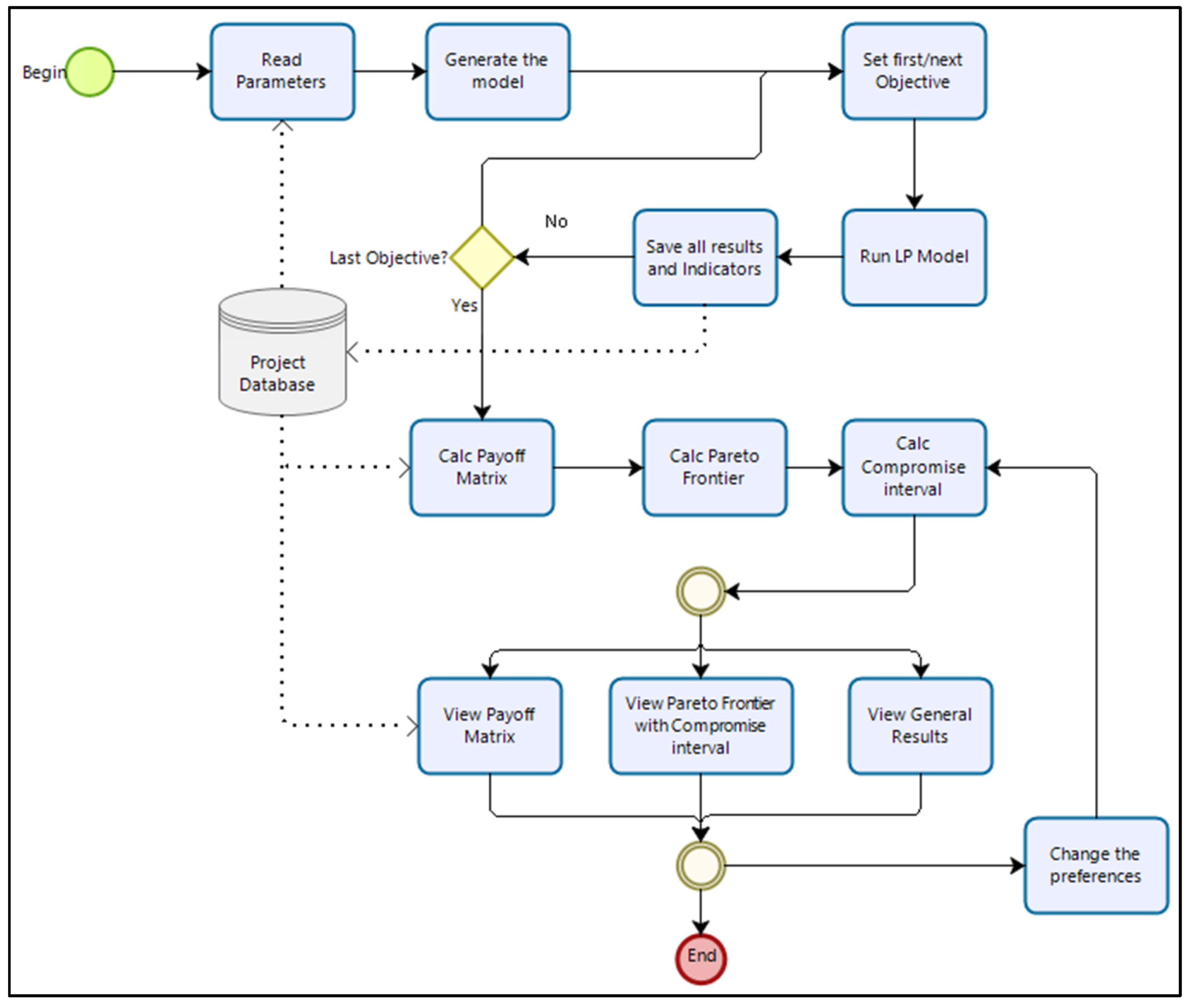
2.2.3. Compromise Programming (CP)
- The user inputs how many points he wants to calculate in the Pareto-efficient set. The user should set as many points as possible depending on the time each run (to obtain one point) takes.
- Romero®
- o
- distributes those points between the best and worst values of each attribute,
- o
- runs the MOLP model to calculate the efficient point using the constraint methodology,
- o
- saves the results (attribute values, decision variables, and deviation variables) of all points into the database.
- The user updates the decision-makers’ weights for each criterion according to their preferences.
- Romero®:
- o
- calculates L1 and L∞ for each efficient point,
- o
- finds the minimum L1 and minimum L∞ using as SQL to implement and find a proxy of the linear programming models of the statements (A8) and (A9) in Appendix B.
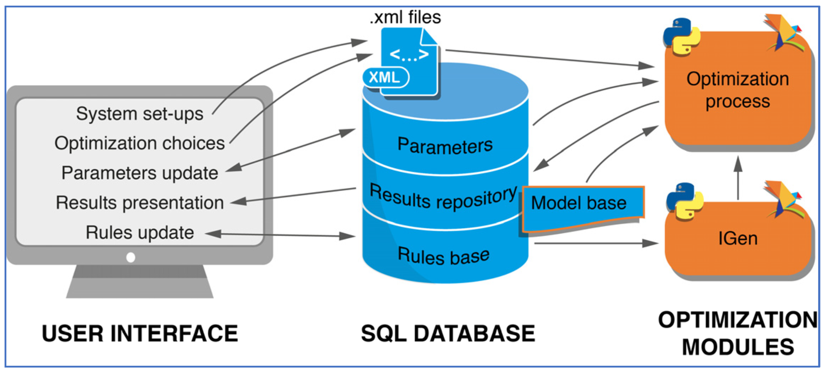
2.2.4. Romero® Architecture
2.3. Romero’s® Application to the Case Study
- regulated wood flow,
- genetic diversification to mitigate risk exposure to plagues and diseases, and
- production sustainability.
3. Results
4. Discussion
5. Conclusions
Author Contributions
Funding
Data Availability Statement
Acknowledgments
Conflicts of Interest
Appendix A. Model Formulation
Appendix B. Compromise Programming Definitions
References
- Wang, S. One hundred faces of sustainable forest management. For. Policy Econ. 2004, 6, 205–213. [Google Scholar] [CrossRef]
- UNDP Human Development Indices and Indicators. 2018 Statistical Update. Rev. Mal. Respir. 2018, 27, 123.
- Secco, L.; Da Re, R.; Pettenella, D.M.; Gatto, P. Why and how to measure forest governance at local level: A set of indicators. For. Policy Econ. 2014, 49, 57–71. [Google Scholar] [CrossRef]
- Bruña-García, X.; Marey-Pérez, M.F. Public participation: A need of forest planning. IForest 2014, 7, 57–71. [Google Scholar] [CrossRef]
- FAO. Global Forest Products 2016: Facts and Figures; FAO: Rome, Italy, 2017. [Google Scholar]
- IBÁ. Relatório 2017. Available online: https://www.iba.org/images/shared/Biblioteca/IBA_RelatorioAnual2017.pdf (accessed on 26 September 2021).
- De Morais, P.H.D.; Longue Júnior, D.; Colodette, J.L.; Morais, E.H.D.C.; Jardim, C.M. Influência da idade de corte de clones de Eucalyptus grandis e híbridos de Eucalyptus grandis × Eucalyptus urophylla na composição química da madeira e polpação kraft. Cienc. Florest. 2017, 27, 237–248. [Google Scholar] [CrossRef]
- Gomide, J.L.; Colodette, J.L.; de Oliveira, R.C.; Silva, C.M. Caracterização tecnológica, para produção de celulose, da nova geração de clones de Eucalyptus do Brasil. Rev. Árvore 2006, 29, 129–137. [Google Scholar] [CrossRef]
- Queiroz, S.C.S.; Gomide, J.L.; Colodette, J.L.; Oliveira, R.C. de Influência da densidade básica da madeira na qualidade da polpa kraft de clones hibrídos de Eucalyptus grandis W. Hill ex Maiden X Eucalyptus urophylla S. T. Blake. Rev. Árvore 2004, 28, 901–909. [Google Scholar] [CrossRef]
- Nobre, S.R.; Rodriguez, L.C.E. Integrating Nursery and Planting Activities. In The Management of Forest Plantations; Borges, G.J., Diaz-Balteiro, L., McDill, E.M., Rodriguez, C.E.L., Eds.; Springer: Dordrecht, The Netherlands, 2014; pp. 347–371. ISBN 978-94-017-8899-1. [Google Scholar]
- Kelty, M.J. The role of species mixtures in plantation forestry. For. Ecol. Manag. 2006, 233, 195–204. [Google Scholar] [CrossRef]
- Kavaliauskas, D.; Fussi, B.; Westergren, M.; Aravanopoulos, F.; Finzgar, D.; Baier, R.; Alizoti, P.; Bozic, G.; Avramidou, E.; Konnert, M.; et al. The Interplay between Forest Management Practices, Genetic Monitoring, and Other Long-Term Monitoring Systems. Forests 2018, 9, 133. [Google Scholar] [CrossRef]
- Mokfienski, A.; Colodette, J.L.; Gomide, J.L.; Carvalho, A.M.M.L. Relative Importance of Wood Density and Carbohydrate Content on Pulping. Cienc. Florest. 2008, 18, 401–413. [Google Scholar] [CrossRef]
- Lopes, G.A.; Garcia, J.N. Basic density and natural moisture content of Eucalyptus saligna Smith, from Itatinga, associated to the population bark patterns. Sci. For. 2002, 1, 13–23. [Google Scholar]
- Gomide, J.L.; Fantuzzi Neto, H.; Regazzi, A.J. Análise de critérios de qualidade da madeira de eucalipto para produção de celulose kraft. Rev. Árvore 2010, 34, 339–344. [Google Scholar] [CrossRef]
- Rodriguez, L.C.E. Programa Cooperativo em Planejamento Florestal—Relatório Final; IPEF-Instituto de Pesquisas e Estudos Florestais: Piracicaba, Brazil, 1988. [Google Scholar]
- Eriksson, L.O.; Garcia-Gonzalo, J.; Trasobares, A.; Hujala, T.; Nordström, E.M.; Borges, J.G. Computerized decision support tools to address forest management planning problems: History and approach for assessing the state of art world-wide. In Computer-Based Tools for Supporting Forest Management: The Experience and the Expertise World-Wide; Borges, J., Nordström, E.-M., Garcia Gonzalo, J., Hujala, T., Eds.; SLU: Umea, Sweden, 2014; pp. 3–25. [Google Scholar]
- Belavenutti, P.; Romero, C.; Diaz-Balteiro, L. A critical survey of optimization methods in industrial forest plantations management. Sci. Agric. 2018, 75, 239–245. [Google Scholar] [CrossRef]
- Acosta, M.; Corral, S. Multicriteria decision analysis and participatory decision support systems in forest management. Forests 2017, 8, 116. [Google Scholar] [CrossRef]
- Esmail, B.A.; Geneletti, D. Multi-criteria decision analysis for nature conservation: A review of 20 years of applications. Methods Ecol. Evol. 2018, 9, 42–53. [Google Scholar] [CrossRef]
- De Castro, M.; Urios, V. A critical review of multi-criteria decision making in protected areas. Econ. Agrar. Y Recur. Nat. Agric. Resour. Econ. 2016, 16, 89–109. [Google Scholar] [CrossRef][Green Version]
- Diaz-Balteiro, L.; González-Pachón, J.; Romero, C. Goal programming in forest management: Customising models for the decision-maker’s preferences. Scand. J. For. Res. 2013, 28, 166–173. [Google Scholar] [CrossRef]
- Diaz-Balteiro, L.; Romero, C. Making forestry decisions with multiple criteria: A review and an assessment. For. Ecol. Manag. 2008, 255, 3222–3241. [Google Scholar] [CrossRef]
- Ananda, J.; Herath, G. A critical review of multi-criteria decision making methods with special reference to forest management and planning. Ecol. Econ. 2009, 68, 2535–2548. [Google Scholar] [CrossRef]
- Giménez, J.C.; Bertomeu, M.; Diaz-Balteiro, L.; Romero, C. Optimal harvest scheduling in Eucalyptus plantations under a sustainability perspective. For. Ecol. Manag. 2013, 291, 367–376. [Google Scholar] [CrossRef]
- Ortiz-Urbina, E.; González-Pachón, J.; Diaz-Balteiro, L. Decision-Making in Forestry: A Review of the Hybridisation of Multiple Criteria and Group Decision-Making Methods. Forests 2019, 10, 375. [Google Scholar] [CrossRef]
- IBÁ Anuário Estatístico do IBÁ. Ano Base 2019. Available online: https://iba.org/datafiles/publicacoes/relatorios/relatorio-iba-2020.pdf (accessed on 26 September 2021).
- FAO FAOSTAT. Available online: http://www.fao.org/faostat/en/#data/FO (accessed on 22 June 2019).
- Camargo, S.A.C.; José, T.; Moura, D. De Influência da dimensão e qualidade dos cavacos na polpação. Influence the size and quality of chips in the pulping. 1 Introdução Revisão Bibliográfica. Rev. Eletrônica Em Gest. Educ. E Tecnol. Ambient. 2015, 19, 813–820. [Google Scholar]
- Alves, I.C.N.; Gomide, J.L.; Colodette, J.L.; Silva, H.D. Caracterização TEcnológica da Madeira de Eucalyptus para produção de Celulose Kraft. Cienc. Florest. 2011, 21, 167–174. [Google Scholar] [CrossRef]
- Clutter, J.L.; Forston, J.C.; Pienaar, L.V.; Brister, G.H.; Bailey, R.L. Timber Management, A Quantitative Approach, 1st ed.; John Wiley & Sons: New York, NY, USA, 1983; ISBN 0-471-02961-0. [Google Scholar]
- Brasil Ministerio da Economia Taxa de Juros Selic. Available online: http://receita.economia.gov.br/orientacao/tributaria/pagamentos-e-parcelamentos/taxa-de-juros-selic (accessed on 23 June 2019).
- Foekel, C.E.B. Rendimentos em celulose sulfato de Eucalyptus spp em função do grau de deslignificação e da densidade da madeira. IPEF Piracicaba 1974, 9, 61–77. [Google Scholar]
- Stape, J.L.; Binkley, D.; Ryan, M.G.; Fonseca, S.; Loos, R.A.; Takahashi, E.N.; Silva, C.R.; Silva, S.R.; Hakamada, R.E.; de Ferreira, J.M.A.; et al. The Brazil Eucalyptus Potential Productivity Project: Influence of water, nutrients and stand uniformity on wood production. For. Ecol. Manag. 2010, 259, 1684–1694. [Google Scholar] [CrossRef]
- Binkley, D.; Campoe, O.C.; Alvares, C.; Carneiro, R.L.; Cegatta, Í.; Stape, J.L. The interactions of climate, spacing and genetics on clonal Eucalyptus plantations across Brazil and Uruguay. For. Ecol. Manag. 2017, 405, 271–283. [Google Scholar] [CrossRef]
- Garcia-Gonzalo, J.; Bushenkov, V.; McDill, M.; Borges, J.G. A decision support system for assessing trade-offs between ecosystem management goals: An application in portugal. Forests 2015, 6, 65–87. [Google Scholar] [CrossRef]
- Garcia-Gonzalo, J.; Borges, J.G.; Palma, J.H.N.; Zubizarreta-Gerendiain, A. A decision support system for management planning of Eucalyptus plantations facing climate change. Ann. For. Sci. 2014, 71, 187–199. [Google Scholar] [CrossRef]
- Borges, J.G.; Diaz-Balteiro, L.; Rodriguez, L.C.E.; McDill, M. The Management of Industrial Forest Plantations, 1st ed.; Borges, J.G., Diaz-Balteiro, L., Rodriguez, L.C.E., Mcdill, M., Eds.; Springer: London, UK, 2014; Volume 33, ISBN 978-94-017-8898-4. [Google Scholar]
- Garcia-Gonzalo, J.; Palma, J.H.N.; Freire, J.P.A.; Tome, M.; Mateus, R.; Rodriguez, L.C.E.; Bushenkov, V. A decision support system for a multi stakeholder’s decision process in a Portuguese National Forest. For. Syst. 2013, 22, 359–373. [Google Scholar] [CrossRef]
- Borges, J.G.; Marques, S.; Garcia-Gonzalo, J.; Rahman, A.U.; Bushenkov, V.; Sottomayor, M.; Carvalho, P.O.; Nordström, E.M. A multiple criteria approach for negotiating ecosystem services supply targets and forest owners’ programs. For. Sci. 2017, 63, 49–61. [Google Scholar] [CrossRef]
- McDill, M. An Overview of Forest Management Planning and Information Management. In The Management of Industrial Forest Plantations; Borges, G.J., Diaz-Balteiro, L., McDill, E.M., Rodriguez, C.E.L., Eds.; Springer: Dordrecht, The Netherlands, 2014; pp. 27–59. ISBN 978-94-017-8899-1. [Google Scholar]
- Borges, J.G.; Nordström, E.M.; Garcia-Gonzalo, J.; Hujala, T.; Trasobares, A. Computer-Based Tools for Supporting Forest Management. The Experience and the Expertise World-Wide, 1st ed.; Department of Forest Resource Management, Swedish University of Agricultural Sciences: Umea, Sweden, 2014. [Google Scholar]
- McDill, M.E.; Toth, S.F.; St:John, R.; Braze, J.; Rebaine, S.A. Comparing Model I and Model II Formulations of Spatially Explicit Harvest Scheduling Models with Adjacency Constraints. For. Sci. 2016, 62, 28–37. [Google Scholar] [CrossRef]
- Garcia-Gonzalo, J.; Pais, C.; Bachmatiuk, J.; Barreiro, S.; Weintraub, A. A progressive hedging approach to solve harvest scheduling problem under climate change. Forests 2020, 11, 224. [Google Scholar] [CrossRef]
- Ware, G.O.; Clutter, J.L. Mathematical Programming System for Management of Industrial Forests. For. Sci. 1971, 17, 428–445. [Google Scholar]
- Johnson, K.N.; Scheurman, H.L. Tequiniques for precribing optimal timber harvest and investment under different objectives—Discussion and synthesis. For. Sci. 1977, 23, a0001–z0001. [Google Scholar]
- Nobre, S.R. Forest Management Decision Support System for Forest Plantation in Brazil: A Multicriteria Apporach. Ph.D. Thesis, Univesidad Politécnica de Madrid, Madrid, Spain, 2019. [Google Scholar]
- Ballestero, E.; Romero, C. Multiple Criteria Decision Making and Its Applications to Economic Problems, 1st ed.; Kluwer Academic Publishers: Boston, MA, USA, 1998; ISBN 0-7923-8238-2. [Google Scholar]
- Romero, C. Teoría de la Decisión Multicriterio, 1st ed.; Alianza Universidad Textos: Madrid, Spain, 1993; ISBN 84-206-8144-X. [Google Scholar]
- Steuer, R.E. Multiple Criteria Optimization—Theory, Computation, and Application, 1st ed.; John Willey & Sons: New York, NY, USA, 1986; ISBN 0271-6232. [Google Scholar]
- Ballestero, E.; Romero, C. A theorem connecting utility function optimization and compromise programming. Oper. Res. Lett. 1991, 10, 421–427. [Google Scholar] [CrossRef]
- Diaz-Balteiro, L.; Belavenutti, P.; Ezquerro, M.; González-Pachón, J.; Nobre, S.R.; Romero, C. Measuring the sustainability of a natural system by using multi-criteria distance function methods: Some critical issues. J. Environ. Manag. 2018, 214, 197–203. [Google Scholar] [CrossRef] [PubMed]
- Beula, T.M.N.; Prasad, G.E. Multiple Criteria Decision Making with Compromise Programming. Int. J. Eng. Sci. Technol. 2012, 4, 4083–4086. [Google Scholar]
- Kanojiya, A.; Nagori, V. Analysis of Architecture and Forms of Outputs of Decision Support Systems Implemented for Different Domains. In Proceedings of the 2018 Second International Conference on Inventive Communication and Computational Technologies (ICICCT), Coimbatore, India, 20–21 April 2018; pp. 346–350. [Google Scholar]
- Reynolds, J.H.; Knutson, M.G.; Newman, K.B.; Silverman, E.D.; Thompson, W.L. A road map for designing and implementing a biological monitoring program. Environ. Monit. Assess. 2016, 188, 399. [Google Scholar] [CrossRef] [PubMed]
- Ezquerro, M.; Pardos, M.; Diaz-Balteiro, L. Operational research techniques used for addressing biodiversity objectives into forest management: An overview. Forests 2016, 7, 299. [Google Scholar] [CrossRef]
- Segura, M.; Maroto, C.; Belton, V.; Ginestar, C. A New Collaborative Methodology for Assessment and Management of Ecosystem Services. Forests 2015, 6, 1696–1720. [Google Scholar] [CrossRef]
- Diaz-Balteiro, L.; González-Pachón, J.; Romero, C. Measuring systems sustainability with multi-criteria methods: A critical review. Eur. J. Oper. Res. 2016, 258, 607–616. [Google Scholar] [CrossRef]
- Rodriguez, L.C.E.; Nobre, S.R. The Use of Forest Decision support System in Brazil. In Computer-Based Tools for Supporting Forest Management. The Experience World-Wide; Borges, J.G., Eriksson, L.O., Nordström, E.M., Garcia-Gonzalo, J., Eds.; Department of Forest Resource Management, Swedish University of Agricultural Sciences: Uppsala, Sweden, 2014; pp. 33–47. [Google Scholar]


| Area | 21,400 ha | ||
| Management units | 18 | ||
| Area of each unit | From 500 to 1900 ha | ||
| Allowable harvest ages | 6 and 7 years old | ||
| Silvicultural costs | R$9500.00/ha | ||
| Pulpwood price | R$50/m3 | ||
| Discount rate | 7% | ||
| Groups | Average Productivity (m3/ha.year at 7 years old) | Average Wood Density (kg/m3 at 7 years old) | |
| Species Eucalyptus spp. | GenMat1 | 42 | 580 |
| GenMat2 | 48 | 500 | |
| GenMat3 | 52 | 420 | |
| Scenarios | Allowable Ages |
|---|---|
| 216 | 5, 6, 7 |
| 217 | 6, 7, 8 |
| 218 | 6, 7, 8, 9 |
| Mill Requirements | Implementation |
|---|---|
| Regulated wood flow | From period 2 onwards No decrease above 10% No increase above 25% |
| Genetic material safety | 60% maximum area for any GenMat type 20% minimum area for any GenMat type |
| Production sustainability | Age class control 10% flexibility |
| Objectives | Objective Description | Attribute (Accounting Variable) |
|---|---|---|
| MaxNPV | Maximize Net Present Value | xTotalNPV |
| MaxMillPrd | Maximize Mill Production | xTotalMillPrd |
| MaxStck | Maximize Final Stock | xTotalStock |
| Scenario | Ages (Years) | Highest NPV (M R$) | Lowest NPV (M R$) | Forest NPV Reduction | Highest Pulp Production (K t) | Lowest Pulp Production (K t) | Mill Production Reduction |
|---|---|---|---|---|---|---|---|
| 216 | 5, 6, 7 | 262,293 | 224,246 | 16.97% | 5149 | 4845 | 6.29% |
| 217 | 6, 7, 8 | 266,445 | 232,677 | 14.51% | 5022 | 4671 | 7.51% |
| 218 | 6, 7, 8, 9 | 266,612 | 232,677 | 14.58% | 5022 | 4656 | 7.85% |
| Scenarios | ||||
|---|---|---|---|---|
| 216 | 217 | 218 | ||
| number of constraints | 53,304 | 23,280 | 38,049 | |
| number of variables | 76,588 | 33,145 | 55,096 | |
| time consumption (min:s) | ||||
| iGen | 00:01.0 | 00:01.0 | 00:02.0 | |
| Mem structure optimization | 00:01.0 | 00:00.0 | 00:00.0 | |
| Building abstract model | 00:01.0 | 00:00.0 | 00:00.0 | |
| Building concrete model | 21:21.0 | 03:44.0 | 12:33.0 | |
| Solving 1st criteria and save results | MaxNPV | 00:19.0 | 00:07.0 | 00:11.0 |
| Solving 2nd criteria and save results | MaxStck | 00:18.0 | 00:06.0 | 00:12.0 |
| Solving 3rd criteria and save results | MaxMillPrd | 00:19.0 | 00:07.0 | 00:12.0 |
| Criteria | Clear-Cut Area (ha) | Production (K m3) | Productivity (m3/ha) | %Max Stock | Forest NPV (M R$) | Pulp Production (K t) | Final Stock (K m3) |
|---|---|---|---|---|---|---|---|
| MaxNPV | 82,992 | 19,708 | 237 | 88.42% | 266,445 | 4671 | 624 |
| MaxMillPrd | 84,622 | 18,856 | 223 | 91.79% | 232,677 | 5022 | 648 |
| MaxStck | 81,695 | 18,335 | 224 | 239,414 | 4801 | 706 |
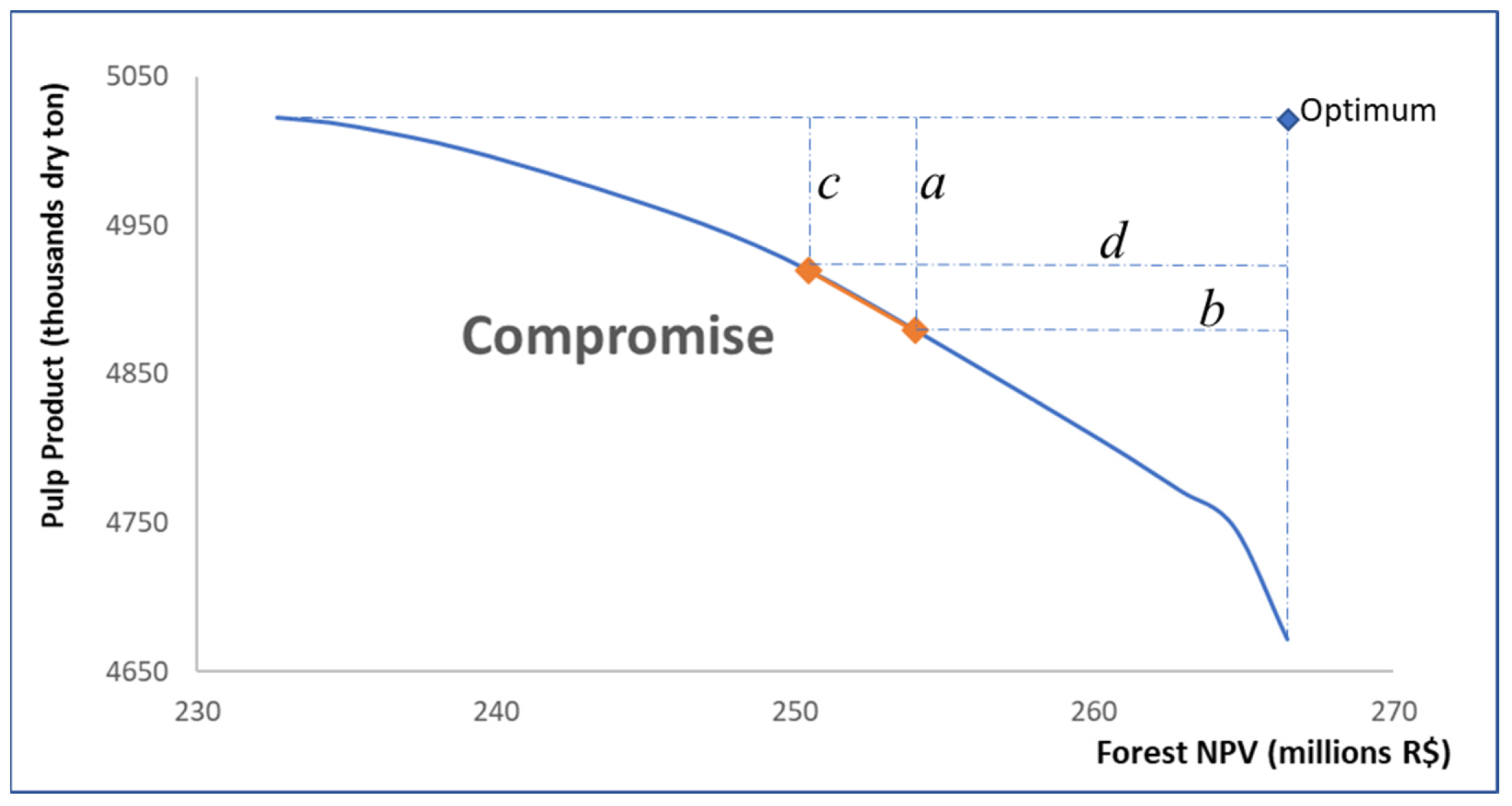
| Point | Criterion | Value | Best Value | Worst Value | Interval | Distance | Sum | Max | ||
|---|---|---|---|---|---|---|---|---|---|---|
| (M R$) | ||||||||||
| 9 | MaxMillPrd | 4879 | 5022 | 4671 | 350 | a | 0.4071 | |||
| 9 | MaxNPV | 254,004 | 266,445 | 232,677 | 33,767 | b | 0.3684 | 0.7755 | 0.4071 | L∞ |
| 10 | MaxMillPrd | 4900 | 5022 | 4671 | 350 | 0.3479 | ||||
| 10 | MaxNPV | 252,227 | 266,445 | 232,677 | 33,767 | 0.4210 | 0.7690 | 0.4210 | ||
| 11 | MaxMillPrd | 4919 | 5,022 | 4671 | 350 | c | 0.2929 | |||
| 11 | MaxNPV | 250,449 | 266,445 | 232,677 | 33,767 | d | 0.4736 | 0.7666 | 0.4736 | L1 |
Publisher’s Note: MDPI stays neutral with regard to jurisdictional claims in published maps and institutional affiliations. |
© 2021 by the authors. Licensee MDPI, Basel, Switzerland. This article is an open access article distributed under the terms and conditions of the Creative Commons Attribution (CC BY) license (https://creativecommons.org/licenses/by/4.0/).
Share and Cite
Nobre, S.R.; Diaz-Balteiro, L.; Rodriguez, L.C.E. A Compromise Programming Application to Support Forest Industrial Plantation Decision-Makers. Forests 2021, 12, 1481. https://doi.org/10.3390/f12111481
Nobre SR, Diaz-Balteiro L, Rodriguez LCE. A Compromise Programming Application to Support Forest Industrial Plantation Decision-Makers. Forests. 2021; 12(11):1481. https://doi.org/10.3390/f12111481
Chicago/Turabian StyleNobre, Silvana Ribeiro, Luis Diaz-Balteiro, and Luiz Carlos Estraviz Rodriguez. 2021. "A Compromise Programming Application to Support Forest Industrial Plantation Decision-Makers" Forests 12, no. 11: 1481. https://doi.org/10.3390/f12111481
APA StyleNobre, S. R., Diaz-Balteiro, L., & Rodriguez, L. C. E. (2021). A Compromise Programming Application to Support Forest Industrial Plantation Decision-Makers. Forests, 12(11), 1481. https://doi.org/10.3390/f12111481