Optimal Harvesting Decision Paths When Timber and Water Have an Economic Value in Uneven Forests


Abstract
1. Introduction
2. Materials and Methods
2.1. Forest Growth Model for Uneven-Aged Stands
2.2. Estimation of the Ingrowth and Up-Growth Matrix Parameters
2.3. Forest Management Optimization Model
2.3.1. The Harvesting/Thinning Decision Model
2.3.2. Forest State Dynamics
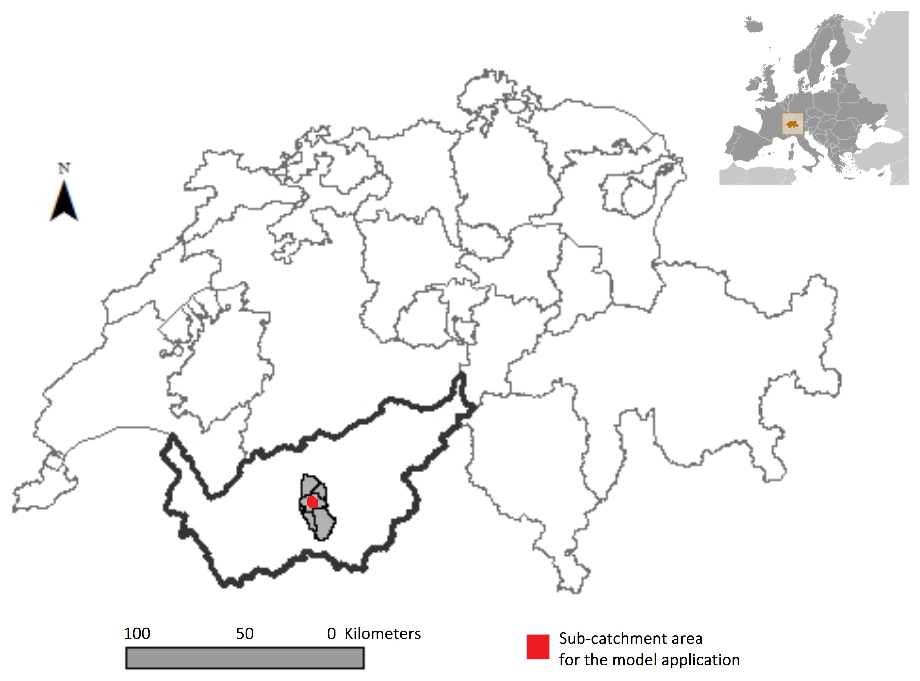
2.4. Case Study for the Application of the Modeling Framework
2.5. Valuation of Timber and Water-Related Ecosystem Services
2.6. Ecohydrological Functions
3. Results and Discussion
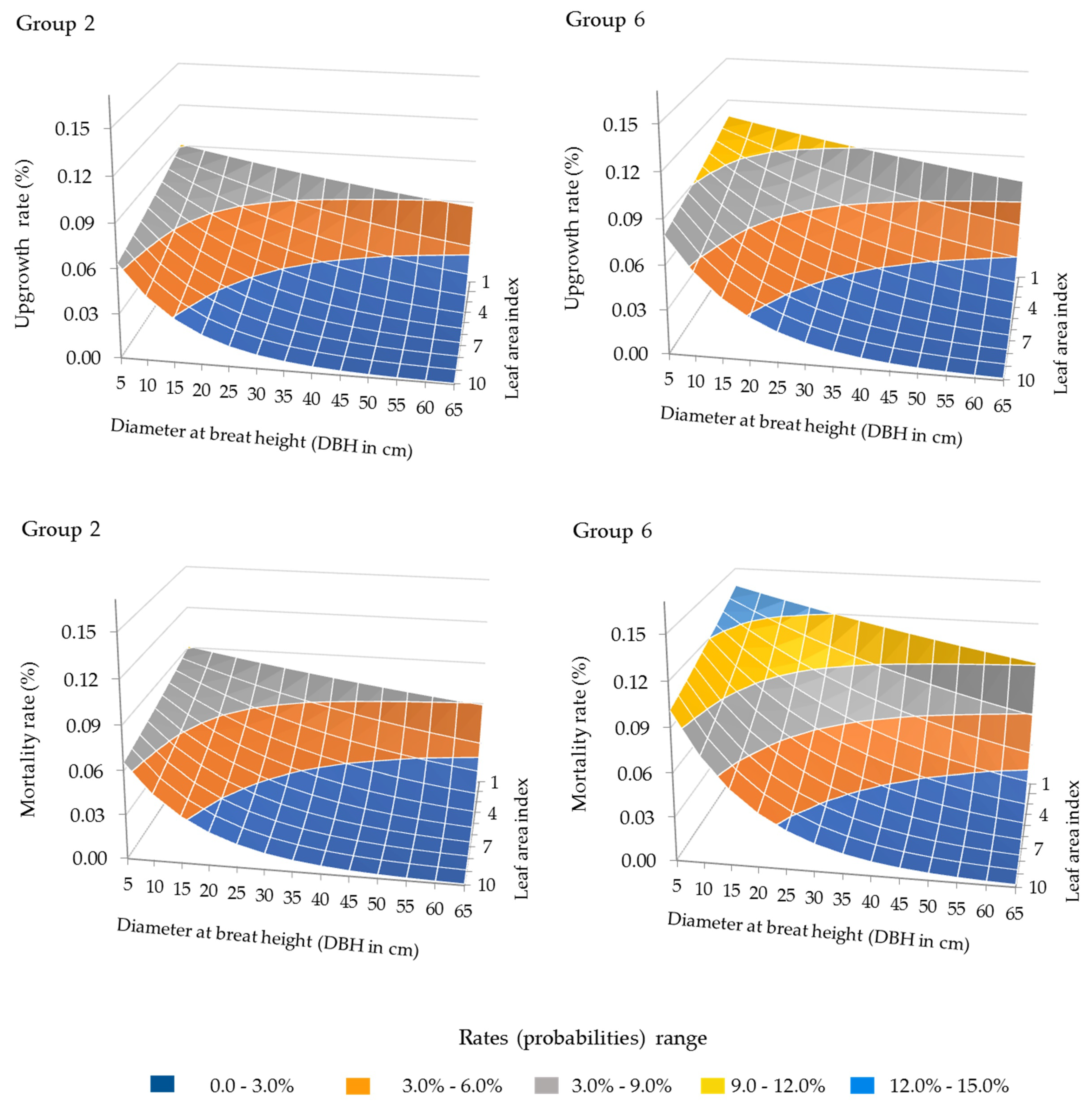
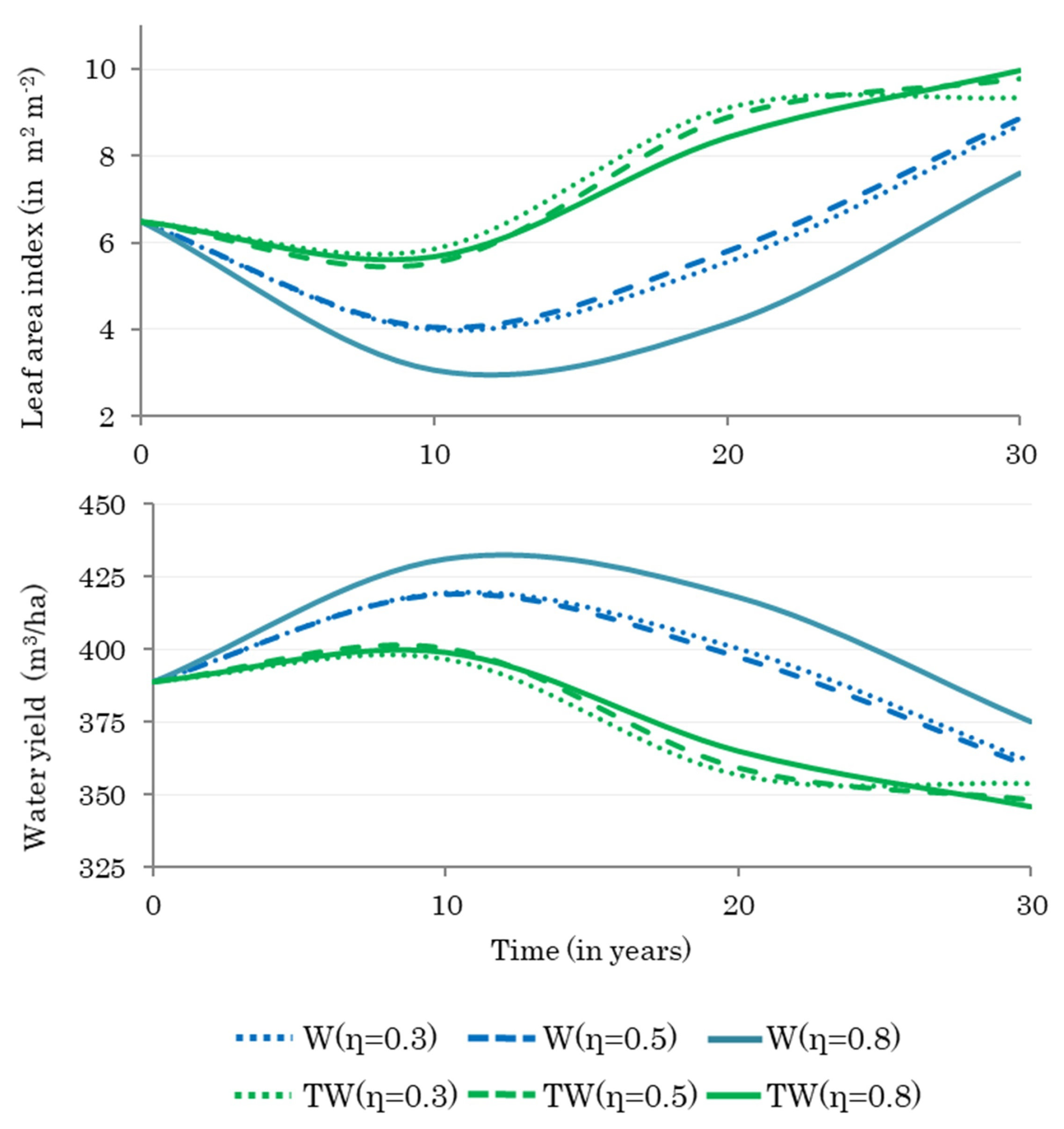
3.1. Forest Growth Functions
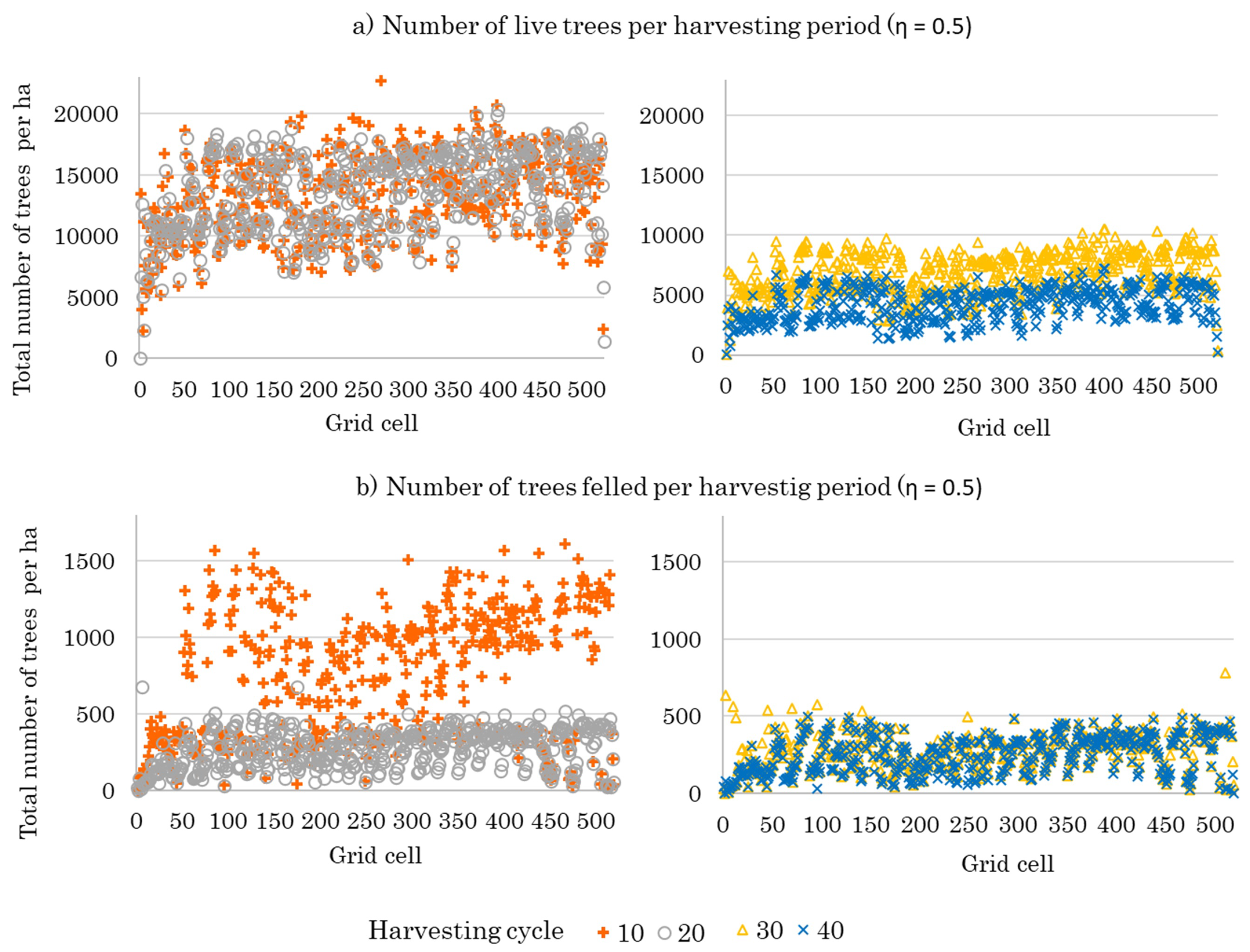
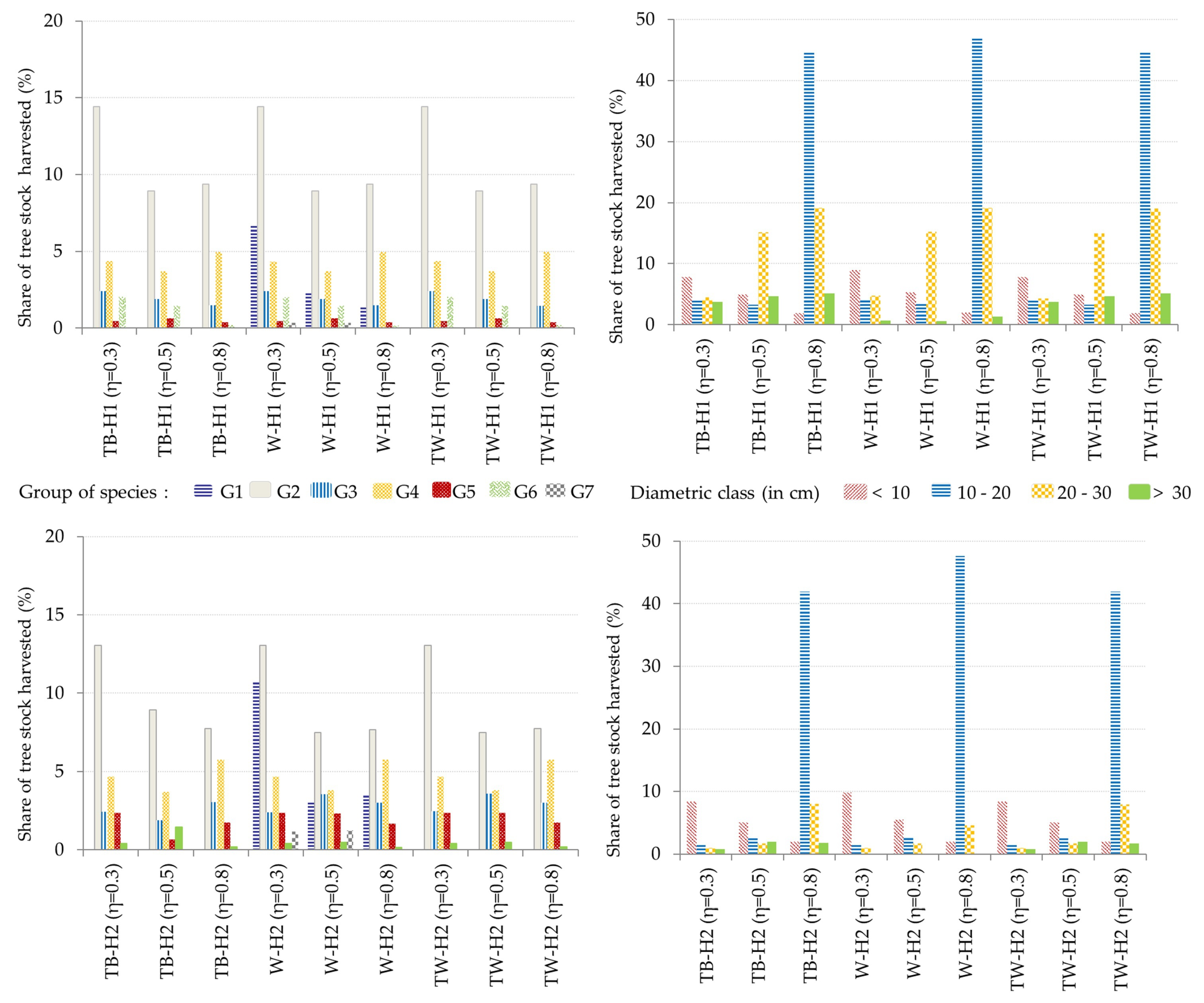
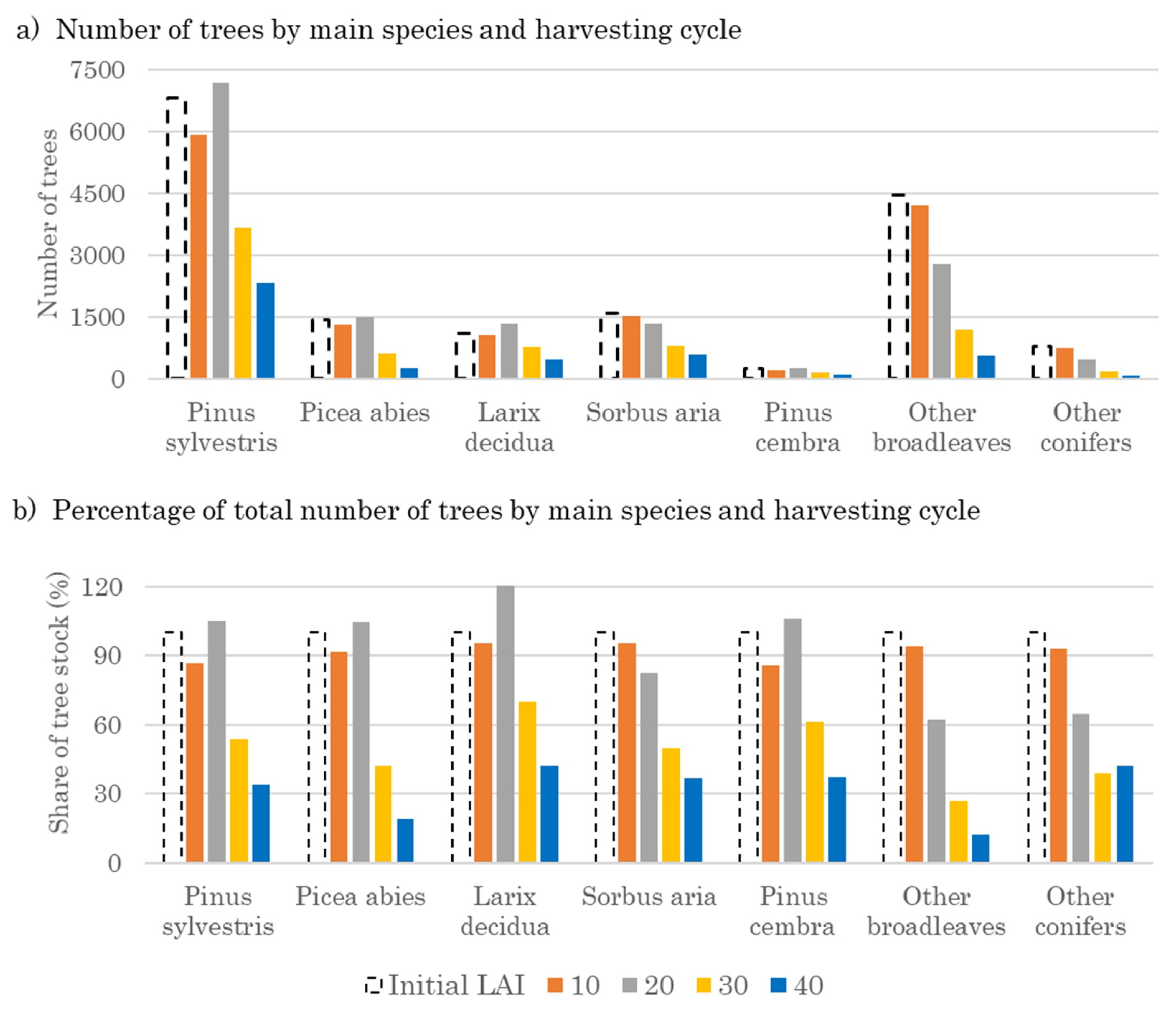
3.2. Optimal Forest Structures and Management When Timber and Water Benefits Are Maximized
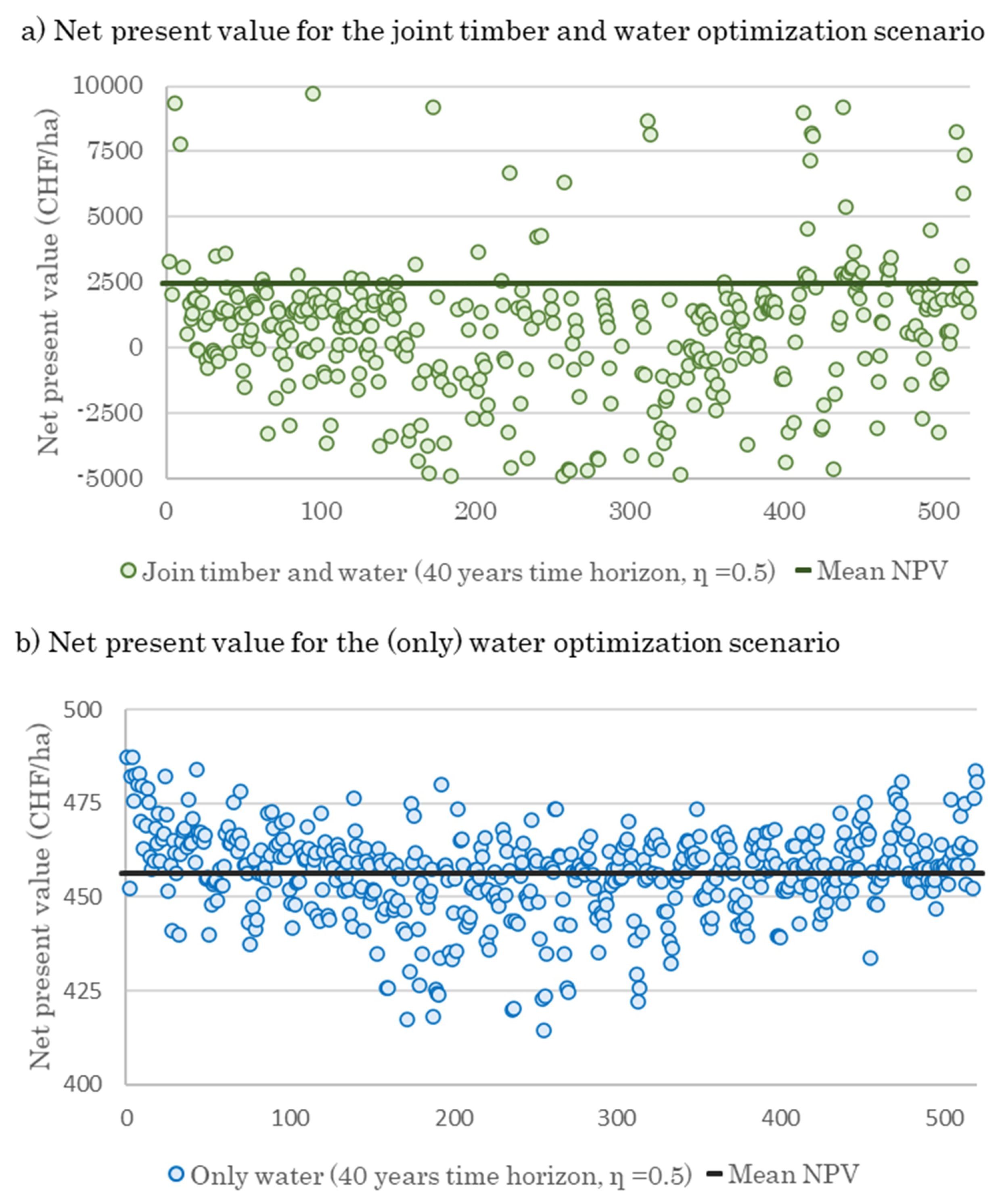
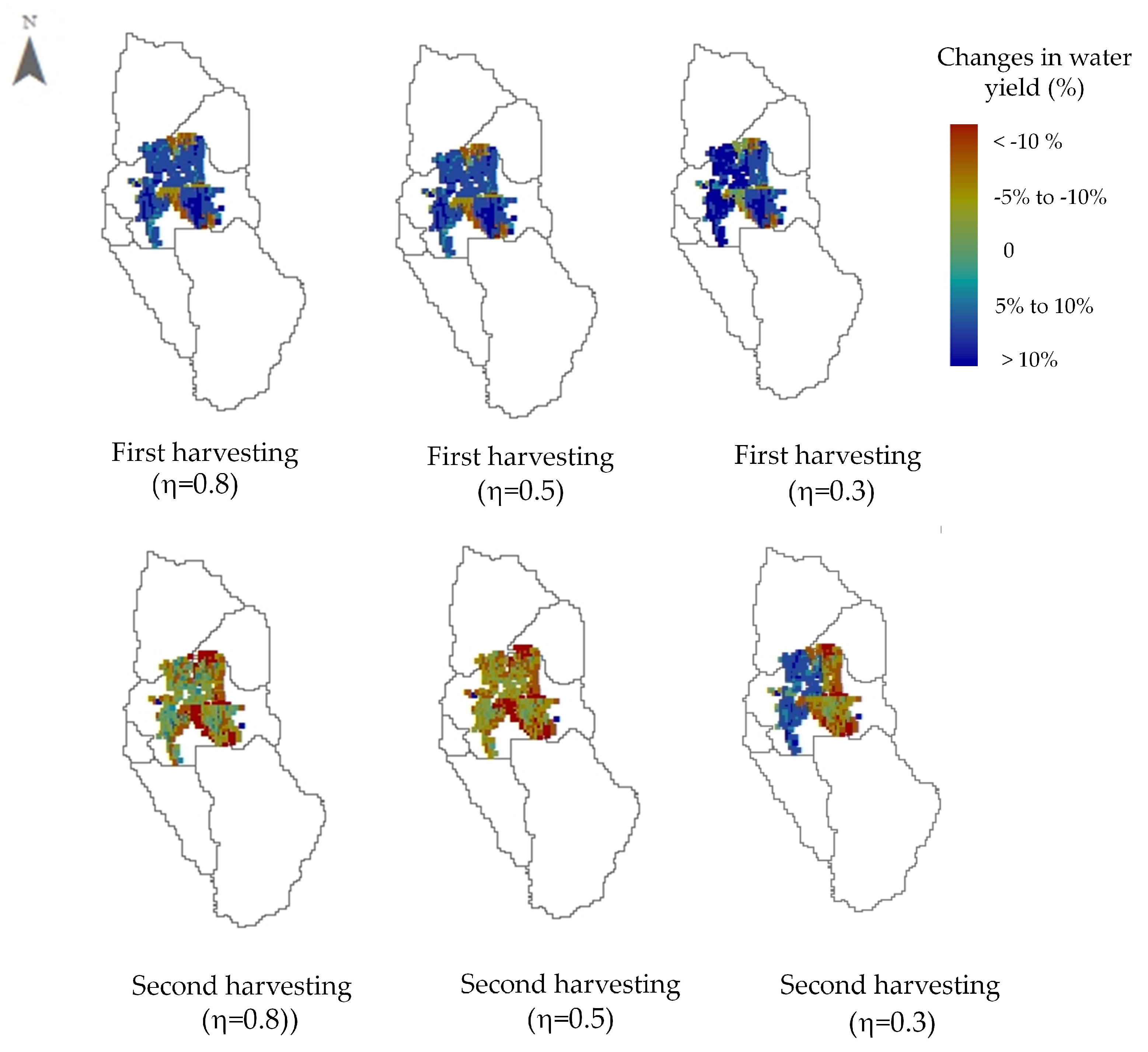
3.3. Effect of Optimal Harvesting Decisions on Water Yield
4. Conclusions
Supplementary Materials
Author Contributions
Funding
Acknowledgments
Conflicts of Interest
References
- Faustmann, M. Berechnung des Wertes welchen Waldboden sowie noch nicht haubare Holzbestaende fuer die Waldwirtschaft besitzen. Allg. Forst- Und Jagd-Zaitung 1849, 15, 441–455. [Google Scholar]
- Samuelson, P. Economics of Forestry in an Evolving Society. Econ. Inq. 1976, 14, 466–492. [Google Scholar] [CrossRef]
- Sinha, A.; Rämö, J.; Malo, P.; Kallio, M.; Tahvonen, O. Optimal management of naturally regenerating uneven-aged forests. Eur. J. Oper. Res. 2017, 256, 886–900. [Google Scholar] [CrossRef]
- Hanewinkel, M. The role of economic models in forest management. Cab Rev. Perspect. Agric. Vet. Sci. Nutr. Nat. Resour. 2009, 4, 1–10. [Google Scholar] [CrossRef]
- Kuuluvainen, T.; Tahvonen, O.; Aakala, T. Even-aged and uneven-aged forest management in boreal fennoscandia: A review. Ambio 2012, 41, 720–737. [Google Scholar] [CrossRef]
- Nolet, P.; Kneeshaw, D.; Messier, C.; Béland, M. Comparing the effects of even- and uneven-aged silviculture on ecological diversity and processes: A review. Ecol. Evol. 2018, 8, 1217–1226. [Google Scholar] [CrossRef]
- Tahvonen, O. Optimal Choice between Even- and Unevenaged Forest Management Systems; Working Paper of the Finnish Forest Research Institute 60; Finnish Forest Research Institute: Vantaa, Finland, 2007; ISBN 978-951-40-2062-9. [Google Scholar]
- Tahvonen, O.; Pukkala, T.; Laiho, O.; Lähde, E.; Niinimäki, S. Optimal management of uneven-aged Norway spruce stands. For. Ecol. Manag. 2010, 260, 106–115. [Google Scholar] [CrossRef]
- Tahvonen, O.; Rämö, J.; Mönkkönen, M. Economics of mixed-species forestry with ecosystem services. Can. J. For. Res. 2019, 49, 1219–1232. [Google Scholar] [CrossRef]
- Rosa, R.; Soares, P.; Tomé, M. Evaluating the Economic Potential of Uneven-aged Maritime Pine Forests. Ecol. Econ. 2018, 143, 210–217. [Google Scholar] [CrossRef]
- Buongiomo, J. Generalization of Faustmanrfs. Formula for Stochastic Forest Growth and Prices with Markov Decision Process Models. For. Sci. 2001, 47, 466–474. [Google Scholar]
- Schou, E.; Jacobsen, J.B.; Kristensen, K.L. An economic evaluation of strategies for transforming even-aged into near-natural forestry in a conifer-dominated forest in Denmark. For. Policy Econ. 2012, 20, 89–98. [Google Scholar] [CrossRef]
- Usher, M. A matrix approach to the management of renewable resources, withspecial reference to selection forests. J. Appl. Ecol. 1966, 3, 355–367. [Google Scholar] [CrossRef]
- Adam, D.M.; Ek, A.R. Optimizing the management of Uneven-aged Forest Stands. Can. J. For. Res. 1974, 4, 274–287. [Google Scholar] [CrossRef]
- Jacobsen, J.B.; Jensen, F.; Thorsen, B.J. Forest Value and Optimal Rotations in Continuous Cover Forestry. Environ. Resour. Econ. 2018, 69, 713–732. [Google Scholar] [CrossRef]
- Haight, R.G.; Brodie, J.D.; Adams, D.M. Optimizing the sequence of diameter distributions and selection harvests for uneven-aged stand management. For. Sci. 1985, 31, 451–462. [Google Scholar]
- Buongiorno, J.; Michie, B.R. A matrix model of uneven-aged forest management. For. Sci. 1980, 22, 609–625. [Google Scholar] [CrossRef]
- Haight, R.G.; Monserud, R.A. Optimizing any-aged management of mixed species stands: II. Effects of decision criteria. For. Sci. 1990, 36, 125–144. [Google Scholar]
- Yang, F.; Kant, S. Forest-level analyses of uneven-aged hardwood forests. Can. J. For. Res. Rev. Can. Rech. For. 2008, 38, 376–393. [Google Scholar] [CrossRef]
- Buongiorno, J.; Peyron, J.L.; Houllier, F.; Bruciamacchie, M. Growth and Management of Forests in the French Jura: Implications for Economic Returns and Tree Diversity. For. Sci. 1995, 41, 397–429. [Google Scholar]
- Indrajaya, Y.; van der Werf, E.; Weikard, H.P.; Mohren, F.; van Ierland, E.C. The potential of REDD+ for carbon sequestration in tropical forests: Supply curves for carbon storage for Kalimantan, Indonesia. For. Policy Econ. 2016, 71, 1–10. [Google Scholar] [CrossRef]
- Parajuli, R.; Chang, S.J. Carbon sequestration and uneven-aged management of loblolly pine stands in the Southern USA: A joint optimization approach. For. Policy Econ. 2012, 22, 65–71. [Google Scholar] [CrossRef]
- Creed, I.F.; van Noordwijk, M. Forest and Water on a Changing Planet: Vulnerability, Adaptation and Governance Opportunities A Global Assessment Report; Technical Report; IUFRO World Series; IUFRO: Viena, Austria, 2018; Volume 38. [Google Scholar]
- Sun, G.; Vose, J. Forest Management Challenges for Sustaining Water Resources in the Anthropocene. Forests 2016, 7, 68. [Google Scholar] [CrossRef]
- Creed, I.F.; Jones, J.J.; Garderen, E.A.V.; Ellison, D.; Mcnulty, S.G.; Noordwijk, M.V.; Vira, B.; Wei, X.; Bishop, K.; Blanco, J.A.; et al. Managing forests for both downstream and downwind water. Front. For. Glob. Chang. 2019, 2, 1–8. [Google Scholar] [CrossRef]
- Price, J.I.; Heberling, M.T. The Effects of Source Water Quality on Drinking Water Treatment Costs: A Review and Synthesis of Empirical Literature. Ecol. Econ. 2018, 151, 195–209. [Google Scholar] [CrossRef]
- Filoso, S.; Bezerra, M.O.; Weiss, K.C.B.; Filoso, S.; Palmer, M.A. Impacts of forest restoration on water yield: A systematic review. PLoS ONE 2017, 12, 1–26. [Google Scholar] [CrossRef]
- Williams, C.A.; Reichstein, M.; Buchmann, N.; Baldocchi, D.; Beer, C.; Schwalm, C.; Wohlfahrt, G.; Hasler, N.; Bernhofer, C.; Foken, T.; et al. Climate and vegetation controls on the surface water balance: Synthesis of evapotranspiration measured across a global network of flux towers. Water Resour. Res. 2012, 48, 1–13. [Google Scholar] [CrossRef]
- Ovando, P.; Brouwer, R. A review of economic approaches modeling the complex interactions between forest management and watershed services. For. Policy Econ. 2019, 100, 164–176. [Google Scholar] [CrossRef]
- Boncina, A. History, current status and future prospects of uneven-aged forest management in the Dinaric region: An overview. Forestry 2011, 84, 467–478. [Google Scholar] [CrossRef]
- Mina, M.; Martin-Benito, D.; Bugmann, H.; Cailleret, M. Forward modeling of tree-ring width improves simulation of forest growth responses to drought. Agric. For. Meteorol. 2016, 221, 13–33. [Google Scholar] [CrossRef]
- Elkin, C.; Giuggiola, A.; Rigling, A.; Bugmann, H. Short- and long-term efficacy of forest thinning to mitigate derought impacts in mountain forest. Ecol. Appl. 2015, 25, 1083–1098. [Google Scholar] [CrossRef]
- Speich, M.J.; Zappa, M.; Lischke, H. Sensitivity of forest water balance and physiological drought predictions to soil and vegetation parameters—A model-based study. Environ. Model. Softw. 2018, 102, 213–232. [Google Scholar] [CrossRef]
- Bigler, C.; Bräker, O.U.; Bugmann, H.; Dobbertin, M.; Rigling, A. Drought as an inciting mortality factor in scots pine stands of the Valais, Switzerland. Ecosystems 2006, 9, 330–343. [Google Scholar] [CrossRef]
- Calder, I. Land Use Impacts on Water Resources; Technical Report; FAO: Rome, Italy, 2000. [Google Scholar]
- Virgilietti, P.; Buongiorno, J. Modeling forest growth with management data: A matrix approach for the Italian Alps. Silva Fenn. 1997, 31, 27–42. [Google Scholar] [CrossRef]
- Speich, M.J.; Zappa, M.; Scherstjanoi, M.; Lischke, H. FORests and HYdrology under Climate Change in Switzerland v1.0: A spatially distributed model combining hydrology and forest dynamics. Geosci. Model Dev. 2020, 13, 537–564. [Google Scholar] [CrossRef]
- Lischke, H.; Zimmermann, N.E.; Bolliger, J.; Rickebusch, S.; Löffler, T.J. TreeMig: A forest-landscape model for simulating spatio-temporal patterns from stand to landscape scale. Ecol. Model. 2006, 199, 409–420. [Google Scholar] [CrossRef]
- Gurtz, J.; Baltensweiler, A.; Lang, H. Spatially distributed hydrotope-based modelling of evapotranspiration and runoff in mountainous basins. Hydrol. Process. 1999, 13, 2751–2768. [Google Scholar] [CrossRef]
- Keles, S.; Baskent, E. Joint production of timber and water: A case study. Water Policy 2011, 13, 535–546. [Google Scholar] [CrossRef]
- Kucuker, D.M.; Baskent, E.Z. Evaluation of Forest Dynamics Focusing on Various Minimum Harvesting Ages in Multi-Purpose Forest Management Planning. For. Syst. 2015, 24, 1–10. [Google Scholar]
- Cerdá, E.; Martín, D. Optimal control for forest management and conservation analysis in dehesa ecosystems. Eur. J. Oper. Res. 2013, 227, 515–526. [Google Scholar] [CrossRef]
- Buongiorno, J.; Gilless, J. Decision Methods for Forest Resource Management; Academic Press: San Diego, CA, USA, 2003. [Google Scholar]
- Fisher, I. The Theory of Interest; Macmillan: New York, NY, USA, 1930. [Google Scholar]
- Bugmann, H. On the Ecology of Mountainous Forests in a Changing Climate. A Simulation Study. Ph.D. Thesis, ETH Zurich, Zurich, Switzerland, 1994. [Google Scholar]
- Federal Statistical Office. Economic Valuation of Standing Timber Stock in Switzerland; Technical Report Agriculture and Forestry; FSO: Neufchatel, Switzerland, 2016.
- Federal Statistical Office. Swiss Consumer Price Index (CPI). 2017. Available online: www.lik.bfs (accessed on 1 August 2018).
- UNSD. System of Environmental-Economic Accounting: A Central Framework; Technical Report 10-11; United Nation: New York, NY, USA; European Commision: Ispra, Italy; FAO: Rome, Italy; OECD: Paris, France; World Bank Group: Washington, DC, USA, 2014. [Google Scholar]
- Reynard, E.; Bonriposi, M. Water Use Managemet in Dry Mountains in Switzerland. The Case of Crans-Montana-Sierre Area. In The Impact of Urbanization, Insdustrial, Agricultural and Forest Technologies on the Natural Environment; Mnemeényi, M., Heil, B., Eds.; Nyugat-Magyarorszagi Egyetem: Sopron, Hungray, 2012; pp. 281–301. [Google Scholar]
- Canton Valais. Le Valais en Chiffres/Das Wallis in Zahlen 2016; Technical Report; Office Cantonal De Statistique et de Péréquation: Sion, Switzerland, 2017. [Google Scholar]
- Blanc, P.; Schädler, B. Water in Switzerland—An Overview. Federal Office for the Environment (FOEN); Technical Report; Swiss Hydrological Commission: Geneva, Switzerland, 2014. [Google Scholar]
- Becken, S. Water equity - Contrasting tourism water use with that of the local community. Water Resour. Ind. 2014, 7–8, 9–22. [Google Scholar] [CrossRef]
- Alpiq Suisse. La Centrale de la Navizence; Forces Motrices de la Gougra, SA: Barrage de Moiry, Switzerland, 2014. [Google Scholar]
- Barry, M.; Baur, P.; Gaudard, L.; Giuliani, G.; Hediger, W.; Schillinger, M.; Schumann, R.; Voegeli, G.; Weigt, H.; Barry, M.; et al. The Future of Swiss Hydropower A Review on Drivers and Uncertainties The Future of Swiss Hydropower A Review on Drivers and Uncertainties; WWZ Working Paper 2015/11; WWZ: Basel, Switzerland, 2015. [Google Scholar]
- Canton Valais. Inventaire du Tourisme Valasain 2015. Observatoire Valasain du Tourisme 2015. Technical Report. 2015. Available online: https://www.tourobs.ch/fr/publications/publications (accessed on 18 December 2017).
- Faust, A.K.; Baranzini, A. The economic performance of Swiss drinking water utilities. J. Product. Anal. 2014, 41, 383–397. [Google Scholar] [CrossRef][Green Version]
- SGWA. Resultats Statistiques Des Distributeurs d’eau en Suisse: Anne 2015; Technical Report; Swiss Water Partenership: Zurich, Switzerland, 2015.
- Agridea; FiBL. Marges Brutes. Modölisation 2017; Technical Report; Swiss Association for the Development of Rural Areas (AGRIDEA) and Research Institute for Organic Agriculture (FiBL): Eschikon, Switzerland, 2017. [Google Scholar]
- Faust, A.K.; Gonseth, C.; Vielle, M. The economic impact of climate-driven changes in water availability in Switzerland. Water Policy 2015, 17, 848–864. [Google Scholar] [CrossRef]
- Forrester, D.I.; Tachauer, I.H.; Annighoefer, P.; Barbeito, I.; Pretzsch, H.; Ruiz-Peinado, R.; Stark, H.; Vacchiano, G.; Zlatanov, T.; Chakraborty, T.; et al. Generalized biomass and leaf area allometric equations for European tree species incorporating stand structure, tree age and climate. For. Ecol. Manag. 2017, 396, 160–175. [Google Scholar] [CrossRef]
- Brunner, I.; Herzog, C.; Dawes, M.A.; Arend, M.; Sperisen, C. How tree roots respond to drought. Front. Plant Sci. 2015, 6, 1–16. [Google Scholar] [CrossRef]
- Chen, Z.; Zhang, Z.; Chen, L.; Cai, Y.; Zhang, H.; Lou, J.; Xu, Z.; Xu, H.; Song, C. Sparse pinus tabuliformis stands have higher canopy transpiration than dense stands three decades after thinning. Forests 2020, 11, 70. [Google Scholar] [CrossRef]


| N | Species | Basal | LAI | LAI by Size Class (%) | LAI | Timber | |||
|---|---|---|---|---|---|---|---|---|---|
| Area | Total | (Diameter Range in cm) | Category | Price | |||||
| (m/ha) | <2.5 | 2.5–10 | 10–30 | >30 | (Cat) | Cat. | |||
| 1 | Abies alba | 0.12 | 0.03 | 0.1 | 0.08 | 0.24 | 0.09 | 2 | 2 |
| 2 | Larix decidua | 2.9 | 0.46 | 1.86 | 2.45 | 3.62 | 0.91 | 5 | 6 |
| 3 | Picea abies | 2.86 | 0.75 | 2.89 | 4.03 | 6.62 | 0.83 | 2 | 4 |
| 4 | Pinus cembra | 1.39 | 0.35 | 0.5 | 0 | 3.07 | 1.65 | 2 | 6 |
| 5 | Pinus montana | 0.25 | 0.14 | 1.73 | 0.9 | 0.16 | 0 | 2 | 4 |
| 6 | Pinus sylvestris | 17.51 | 2.35 | 8.32 | 12.66 | 24.27 | 0.07 | 1 | 2 |
| 7 | Taxus baccata | 0.03 | 0.02 | 0.29 | 0.1 | 0 | 0 | 2 | 7 |
| 8 | Acer campestre | 0.15 | 0.05 | 0.55 | 0.24 | 0.14 | 0 | 5 | 5 |
| 9 | Acer platanoides | 0.41 | 0.11 | 0.87 | 0.47 | 0.71 | 0.02 | 3 | 5 |
| 10 | Acer pseudoplatanus | 0.59 | 0.15 | 1.09 | 0.76 | 0.98 | 0.05 | 3 | 5 |
| 11 | Alnus glutinosa | 0.05 | 0.02 | 0.16 | 0.07 | 0.05 | 0 | 5 | 5 |
| 12 | Alnus incana | 0.14 | 0.05 | 0.25 | 0 | 0.26 | 0.01 | 5 | 5 |
| 13 | Betula pendula | 0.41 | 0.07 | 0.37 | 0 | 0.57 | 0.07 | 4 | 3 |
| 14 | Fagus sylvatica | 0.09 | 0.02 | 0.02 | 0.03 | 0.17 | 0.06 | 3 | 3 |
| 15 | Fraxinus excelsior | 0.22 | 0.05 | 0.37 | 0.24 | 0.28 | 0.02 | 5 | 3 |
| 16 | Populus tremula | 0.11 | 0.03 | 0.32 | 0.16 | 0.12 | 0 | 5 | 3 |
| 17 | Quercus petraea | 0.16 | 0.04 | 0.16 | 0.15 | 0.33 | 0.01 | 3 | 3 |
| 18 | Quercus pubescens | 0.004 | 0.01 | 0.04 | 0.04 | 0.01 | 0 | 3 | 3 |
| 19 | Sorbus aria | 1.73 | 0.38 | 2.85 | 2.48 | 2.28 | 0.01 | 5 | 1 |
| 20 | Sorbus aucuparia | 0.41 | 0.11 | 1.42 | 0.73 | 0.11 | 0.04 | 4 | 1 |
| 21 | Tilia acordata | 0.07 | 0.03 | 0.38 | 0.17 | 0.04 | 0 | 3 | 3 |
| 22 | Tilia platyphyllos | 0.27 | 0.08 | 0.63 | 0.36 | 0.43 | 0 | 3 | 3 |
| 23 | Ulmus scabra | 0.08 | 0.02 | 0.17 | 0.11 | 0.14 | 0 | 3 | 3 |
| Total | 29.96 | 5.29 | |||||||
| Species by Timber Price Category | Diameter at Breast Height (in cm) | |||||
|---|---|---|---|---|---|---|
| Class 3 | Class 4 | Class 5 | Class 6 | Class 7 | Class 8 | |
| (10–19) | (20–29) | (30–39) | (40–49) | (50–59) | (>60) | |
| Timber Prices (in CHF/m) | ||||||
| Group 1 | - | - | - | - | - | - |
| Group 2 | 35.00 | 86.66 | 91.43 | 95.63 | 94.71 | 94.71 |
| (6.18) | (16.73) | (14.18) | (12.18) | (11.23) | (11.23) | |
| Group 3 | 44.22 | 100.22 | 101.27 | 102.72 | 102.72 | 89.18 |
| (6.02) | (10.70) | (14.16) | (20.22) | (20.22) | (19.01) | |
| Group 4 | 37.66 | 102.35 | 105.76 | 118.59 | 115.40 | 115.40 |
| (6.68) | (20.49) | (16.59) | (14.61) | (14.39) | (14.39) | |
| Group 5 | 44.22 | 137.67 | 145.97 | 159.07 | 159.07 | 145.89 |
| (6.02) | (24.05) | (30.25) | (39.54) | (39.54) | (37.98) | |
| Group 6 | 36.02 | 145.61 | 149.42 | 165.32 | 119.18 | 119.18 |
| (6.36) | (29.01) | (26.10) | (20.71) | (14.81) | (14.81) | |
| Group 7 | 42.13 | 42.13 | 42.13 | 42.13 | 42.13 | 42.13 |
| (9.14) | (9.14) | (9.14) | (9.14) | (9.14) | (9.14) | |
| Class | Unit | Quantity (m/unit) | Economic Values (CHF/m) | ||
|---|---|---|---|---|---|
| Revenues | Production Cost | Environmen-Tal Price | |||
| Drinking | resident day | 170 | 1.20 ± 0.46 | 1.05 ± 0.32 | 0.11–0.19 |
| water | tourist night | 199 ± 342 | (0.003–0.006) | ||
| Irrigation | hectare | 827 | 2.04–4.15 | ||
| (0.09–0.15) | |||||
| Hydropower | kW/h | 0.074 | 0.23–0.25 | 0.23–0.25 | 0.013–0.014 |
| Environmental price of water: 0.10 ± 0.02 CHF/m | |||||
| Up-Growth Functions | ||||||
|---|---|---|---|---|---|---|
| Statistics | Coefficient | Robust SE | Coefficient | Robust SE | ||
| Group 1 | Group2 | |||||
| A | 0.099 | *** | 1.784 × 10 | 0.095 | *** | 2.666 × 10 |
| b | −0.008 | *** | 1.393 × 10 | −0.008 | *** | 2.251 × 10 |
| / N | 0.221 | 61,894 | 0.142 | 54,061 | ||
| Group 3 | Group4 | |||||
| A | 0.078 | *** | 1.324 × 10 | 0.087 | *** | 1.11 × 10 |
| b | −0.002 | *** | 7.17 × 10 | −0.004 | *** | 7.89 × 10 |
| / N | 0.154 | 59,136 | 0.197 | 63,637 | ||
| Group 5 | Group 6 | |||||
| A | 0.112 | *** | 3.691 × 10 | 0.076 | *** | 1.344 × 10 |
| b | −0.007 | *** | 2.113 × 10 | −0.006 | *** | 1.299 × 10 |
| / N | 0.158 | 33,173 | 0.197 | 63,637 | ||
| Group 7 | All species | |||||
| A | 0.073 | *** | 1.623 × 10 | 0.08 | *** | 5.838 × 10 |
| b | −0.002 | *** | 8.76 × 10 | −0.004 | *** | 4.03 × 10 |
| / N | 0.113 | 47,362 | 0.146 | 382,900 | ||
| Mortality Functions | ||||||
|---|---|---|---|---|---|---|
| Statistic | Coefficient | Robust SE | Coefficient | Robust SE | ||
| Group 1 | Group2 | |||||
| A | 0.106 | *** | 1.229 × 10 | 0.094 | *** | 1.081 × 10 |
| b | −0.009 | *** | 1.503 × 10 | −0.007 | *** | 1.337 × 10 |
| / N | 0.272 | 70,736 | 0.246 | 61,784 | ||
| Group 3 | Group4 | |||||
| A | 0.115 | *** | 1.004 × 10 | 0.096 | *** | 8.239 × 10 |
| b | −0.003 | *** | 5.73 × 10 | −0.004 | *** | 6.42 × 10 |
| / N | 0.267 | 67,584 | 0.268 | 72,728 | ||
| Group 5 | Group 6 | |||||
| A | 0.142 | *** | 1.615 × 10 | 0.088 | *** | 8.793 × 10 |
| b | −0.007 | *** | 1.241 × 10 | −0.006 | *** | 8.77 × 10 |
| / N | 0.338 | 37,912 | 0.255 | 72,728 | ||
| Group 7 | All species | |||||
| A | 0.137 | *** | 1.339 × 10 | 0.105 | *** | 0.407 × 10 |
| b | −0.004 | *** | 7.34 × 10 | −0.005 | *** | 3.26 × 10 |
| / N | 0.279 | 54,128 | 0.256 | 437,600 | ||
| Ingrowth Functions | ||||||
|---|---|---|---|---|---|---|
| Statistic | Coefficient | Robust SE | Coefficient | Robust SE | ||
| Group 1 | Group 2 | |||||
| A | 0.230 | *** | 0.0162 | 0.271 | *** | 0.0387 |
| b | 0.0804 | *** | 0.0083 | 0.061 | *** | 0.0183 |
| / N | 0.679 | 3,516 | 0.680 | 523 | ||
| Group 3 | Group 4 | |||||
| A | 0.531 | *** | 0.0274 | 0.260 | *** | 0.0142 |
| b | −0.02 | *** | 0.0065 | 0.003 | 0.0069 | |
| / N | 0.686 | 6,770 | 0.474 | 6,394 | ||
| Group 5 | Group 6 | |||||
| A | 0.222 | *** | 0.0163 | 0.932 | *** | 0.014 |
| b | 0.076 | *** | 0.0086 | −0.109 | *** | 0.0025 |
| / N | 0.720 | 3,016 | 0.757 | 6,087 | ||
| Group 7 | All species | |||||
| A | 0.554 | *** | 0.0242 | 0.478 | *** | 0.01 |
| b | −0.046 | *** | 0.0054 | −0.025 | *** | 0.0026 |
| / N | 0.728 | 5,899 | 0.654 | 32,205 | ||
© 2020 by the authors. Licensee MDPI, Basel, Switzerland. This article is an open access article distributed under the terms and conditions of the Creative Commons Attribution (CC BY) license (http://creativecommons.org/licenses/by/4.0/).
Share and Cite
Ovando, P.; Speich, M. Optimal Harvesting Decision Paths When Timber and Water Have an Economic Value in Uneven Forests. Forests 2020, 11, 903. https://doi.org/10.3390/f11090903
Ovando P, Speich M. Optimal Harvesting Decision Paths When Timber and Water Have an Economic Value in Uneven Forests. Forests. 2020; 11(9):903. https://doi.org/10.3390/f11090903
Chicago/Turabian StyleOvando, Paola, and Matthias Speich. 2020. "Optimal Harvesting Decision Paths When Timber and Water Have an Economic Value in Uneven Forests" Forests 11, no. 9: 903. https://doi.org/10.3390/f11090903
APA StyleOvando, P., & Speich, M. (2020). Optimal Harvesting Decision Paths When Timber and Water Have an Economic Value in Uneven Forests. Forests, 11(9), 903. https://doi.org/10.3390/f11090903