An Artificial Intelligence Approach to Predict Gross Primary Productivity in the Forests of South Korea Using Satellite Remote Sensing Data

Abstract

Many process-based models for carbon flux predictions have faced a wide range of uncertainty issues. The complex interactions between the atmosphere and the forest ecosystems can lead to uncertainties in the model result. On the other hand, artificial intelligence (AI) techniques, which are novel methods to resolve complex and nonlinear problems, have shown a possibility for forest ecological applications. This study is the first step to present an objective comparison between multiple AI models for the daily forest gross primary productivity (GPP) prediction using satellite remote sensing data. We built the AI models such as support vector machine (SVM), random forest (RF), artificial neural network (ANN), and deep neural network (DNN) using in-situ observations from an eddy covariance (EC) flux tower and satellite remote sensing data such as albedo, aerosol, temperature, and vegetation index. We focused on the Gwangneung site from the Korea Regional Flux Network (KoFlux) in South Korea, 2006–2015. As a result, the DNN model outperformed the other three models through an intensive hyperparameter optimization, with the correlation coefficient (CC) of 0.93 and the mean absolute error (MAE) of 0.68 g m⁻² d⁻¹ in a 10-fold blind test. We showed that the DNN model also performed well under conditions of cold waves, heavy rain, and an autumnal heatwave. As future work, a comprehensive comparison with the result of process-based models will be necessary using a more extensive EC database from various forest ecosystems.

1. Introduction

Forests, which cover 30% of the Earth’s land area [1], play an essential role in global carbon flux because of their ability to store much more significant amounts of carbon than other terrestrial ecosystems [2]. Terrestrial gross primary productivity (GPP) in the forest ecosystem is the total carbon generated by the photosynthesis of vegetation. GPP refers to the total uptake of carbon dioxide (CO₂) during photosynthesis, which is the primary driver of subsequent ecosystem processes, including vegetation growth and yields [3,4,5]. GPP depends on the change in environmental factors, such as light, temperature, air humidity, air turbulence, and CO₂ concentration. It is also affected by ecosystem physiology, such as nitrogen and proteins supporting leaf carboxylation capacity, the plant structure for exposing photosynthetically active materials to light, and the stomatal restrictions on CO₂ diffusion [6,7]. For measurement and prediction of forest GPP, eddy covariance (EC) flux tower observations, satellite observations, and process-based models are often used. The EC method enables the calculation of forest GPP using the net ecosystem exchange (NEE) derived from direct measurements of the vertical turbulence transport of the atmosphere according to meteorological conditions [8]. More than 500 EC flux observation sites are operated worldwide and provide reasonably accurate estimates of carbon exchange. However, the point-based observations are not sufficient to cover spatially continuous areas [9,10].

Satellite observations and process-based models are used to overcome the limitation of spatial continuity of the EC measurements [11]. However, satellite GPP products may not fully ensure the reliability of data, thus they require a more advanced calibration process suitable for local-scale applications [12]. Process-based models for forest GPP were designed to take account of physiological and environmental factors of forest ecosystems at various scales [13,14,15]. However, it is difficult for the process-based models to handle complex and nonlinear aspects of biological, physiological, and chemical mechanisms of plant organisms under different climatic and topographic conditions. Furthermore, a number of input parameters related to physiology and phenology of vegetation should be precisely calibrated for the process-based models [16,17], which is a very challenging task for local-scale applications.

Forest GPP is a complex and nonlinear problem because its relationships with photosynthetic rates are spatially and temporally heterogeneous. Nowadays, artificial intelligence (AI) approaches are adopted because AI can efficiently handle the problems of nonlinearity and complexity related to forest ecosystems [18]. AI includes machine learning models, such as support vector machine (SVM) and random forest (RF), and neural network models, such as artificial neural network (ANN) and deep neural network (DNN). Previous forest studies using AI methods include the classification of tree species [19,20,21,22] and the estimation of carbon or heat fluxes [23,24,25]. They have sufficiently shown the potential of AI for forest applications. However, a comprehensive comparison between multiple AI models for forest applications has rarely been reported. The FluxCom (Jena, Germany) provides an AI-based operative GPP product with a spatial resolution of 10 km and a temporal resolution of 8 days. The spatial resolution is, however, not sufficient to investigate the GPP of locally inhomogeneous forest ecosystems for the countries with complex terrains such as South Korea.

This study examines the application of AI methods to improve the reliability of the daily GPP predictions for the forest in South Korea using in-situ observations from an EC flux tower and the satellite remote sensing data such as solar radiation, temperature, humidity, and vegetation index. The purposes of this study are (1) to objectively compare the performance of multiple AI models such as SVM, RF, ANN, and DNN for the daily forest GPP in South Korea and (2) to examine the accuracy characteristics according to AI models in relation to different seasons and unexpected weather conditions. We focused on the Gwangneung site from the Korea Regional Flux Network (KoFlux) in South Korea, 2006–2015. Furthermore, this study suggests the possibility of overcoming the spatial limitation of point-based observations and applying the AI model over South Korea.

2. Materials and Methods

2.1. Study Site

The Gwangneung National Arboretum is a warm-temperate deciduous forest stand of which area is approximately 2.2 km² (37°45′25′′ N, 127°09′12′′ E, 340 m above sea level). It is a KoFlux supersite (Figure 1) [26] and belongs to the worldwide FLUXNET network. The radius of the flux tower footprint is about 1 km. For a 30 year period between 1981 and 2010, the mean annual temperature was 11.2 °C, and the mean annual precipitation was 1.502 mm. The precipitation was concentrated during the period between late June and late July due to the influence of the monsoon climate [27]. The site is located on a slope of 10–20°, facing southwest. Gwangneung has been protected to minimize human disturbance over the last 500 years [28]. The forest stand is at the climax and is dominated by 80 to 200 years old Jolcham oak (Quercus serrata) and Loose-flower hornbeam (Carpinus laxiflora) of an average height of about 18 m [29]. The maximum leaf area index (LAI) is approximately 6 m² m⁻² in June.

2.2. Data

2.2.1. Overview

Figure 2 shows a summary of the data used in this study. Input variables for the four AI models (SVM, RF, ANN, and DNN) include downward shortwave radiation (R_s↓), air temperature (T_air), vapor pressure deficit (VPD), and enhanced vegetation index (EVI) obtained from the Moderate-resolution Imaging Spectroradiometer (MODIS) products. GPP is the output value that should be adjusted using the in-situ observations from the EC flux tower.

2.2.2. Eddy Covariance Flux Data

For the ground-truth data at the Gwangneung forest, we accumulated the measurements from an open-path EC and the meteorological system at 40 m above ground. In the EC system, vertical wind speed (ω) was observed by a three-dimensional sonic anemometer (CSAT3, Campbell Scientific, Logan, UT, USA), and the CO₂ concentration (ρc) was measured by an open-path infrared gas analyzer (LI-7500, LI-COR Environmental, Lincoln, NE, USA). These data were collected by a data logger (CR3000, Campbell Scientific, Logan, UT, USA) at the frequency of 10 Hz. Then, the half-hourly vertical CO₂ flux, which is equal to NEE, was calculated from the covariance between the fluctuations in ω and ρc. To derive the NEE from the 10 Hz raw data, we carried out the preprocessing such as air density correction and spike detection. Further, quality control, gap-filling, and nighttime CO₂ flux correction were also conducted according to the standard data-processing protocol of KoFlux [28,29]. The forest GPP was calculated by adding the ecosystem respiration (R_eco) to the NEE. Given that the R_eco is mainly governed by the thermal regime, the R_eco was estimated using the relationship between the temperature and the CO₂ efflux rate derived from nighttime EC measurements. Such efforts should have improved the quality of the GPP data. In addition, meteorological measurements, such as solar radiation, photosynthetically active radiation, net radiation, air temperature, humidity, and precipitation, were sampled every second, averaged over 30 min, and logged in another data logger (CR3000, Campbell Scientific, Logan, UT, USA). They were used as the ancillary variables for the nighttime correction and gap-filling of NEE, and the estimation of R_eco and GPP.

2.2.3. Input Data Processing

MODIS is a satellite sensor that has been developed to monitor Earth’s atmosphere, land, and ocean environment with the launch of Terra and Aqua satellites in 1999 and 2002, respectively [30]. The input data for the AI models (R_s↓, T_air, VPD, and EVI) were derived from multiple MODIS products (

Table 1. Moderate-resolution Imaging Spectroradiometer (MODIS) products used in the calculation of input data for the estimation of daily gross primary productivity (GPP) in the forest of South Korea.

MODIS Product	Data Extracted	Spatial Resolution	Temporal Compositing	Related Input Variable for This Study
MCD43B3	Black- and white-sky albedo for shortwave radiation	1 km	16 days (1)	Rs↓ (3)
MYD04_L2	Aerosol optical depth	10 km	1 day	Rs↓
MYD05_L2	Total column precipitable water	5 km	1 day	Rs↓
MYD07_L2	Air and dew-point temperatures, total ozone, and surface pressure	5 km	1 day	Rs↓, Tair (4), and VPD (5)
MOD13A2 (Terra) MYD13A2 (Aqua)	Enhanced vegetation index	1 km	8 days (2)	EVI (6)

⁽¹⁾ 16 day composite was assigned to each of the 16 days; ⁽²⁾ 8 day composite was interpolated to daily values; ⁽³⁾ downward shortwave radiation; ⁽⁴⁾ air temperature; ⁽⁵⁾ vapor pressure deficit; ⁽⁶⁾ enhanced vegetation index.

). Most of the data have a spatial resolution of 1 to 5 km, which is suitable for the area size (2.2 km²) of the forest stand at the Gwangneung site.

R_s↓, a key component for the land surface energy budget, is primarily used as a meteorological input variable for the retrieval of GPP [31]. To calculate R_s↓, we used a 16 day composite of the black- and the white-sky albedos for shortwave radiation extracted from the MCD43B3 product. For the parameterization of R_s↓, we employed the Bird Model [32] that considers both diffuse and direct radiation. The R_s↓ is then expressed as:

$${\mathrm{R}}_{\mathrm{s}}\downarrow =\left(I_{dir}+I_{dif}\right)/\left(1-a_g·a_s\right)$$

(1)

where $I_{dir}$ is the direct radiation; $I_{dif}$ is the diffuse radiation; $a_g$ is the ground albedo; $a_s$ is the atmospheric albedo. The 16 day albedo was assigned to each of the 16 days because the forest albedo does not significantly vary during a 16 day period [30,33]. From the daily black- and white-sky albedos, the actual albedo was calculated using the MODIS lookup table for a fraction of the diffuse radiation regarding a given solar zenith angle and a 550 nm aerosol optical depth (AOD) [33]. For the parameterization of AOD, we rearranged the daily AOD images using a statistical gap-filling method [34,35]. Total column precipitable water (TPW), total ozone, and surface pressure were also parameterized according to the Bird Model [33]. The daily R_s↓ calculated by this process showed high accuracy with the correlation coefficient (CC) over 0.9 against the Automated Surface Observing System (ASOS) in South Korea [35].

The air and dew-point temperatures from the lowest atmospheric layer (surface layer) were used in the calculation of VPD by subtracting the actual vapor pressure ($e_a$) from the saturated vapor pressure ($e_s$) [36]. The $e_s$ is a function of air temperature, and the $e_a$ can be derived from the $e_s$ and the relative humidity calculated by air and dew-point temperatures.

The EVI can mitigate the saturation problem of the normalized difference vegetation index (NDVI), thus the EVI is commonly used in forest studies because it is more suitable for the representation of vegetation greenness in densely vegetated areas [37,38,39]. The MOD13A2 (Terra) and the MYD13A2 (Aqua) products provide 16 day composites for NDVI and EVI. Because the 16 day periods of the Terra and the Aqua products were crossing each other, we could obtain 8 day composites by combining the Terra and the Aqua products. The 8 day EVI was then converted to daily value using a cubic spline interpolation method because the forest greenness usually shows gradual changes such as the cosine curve during a year.

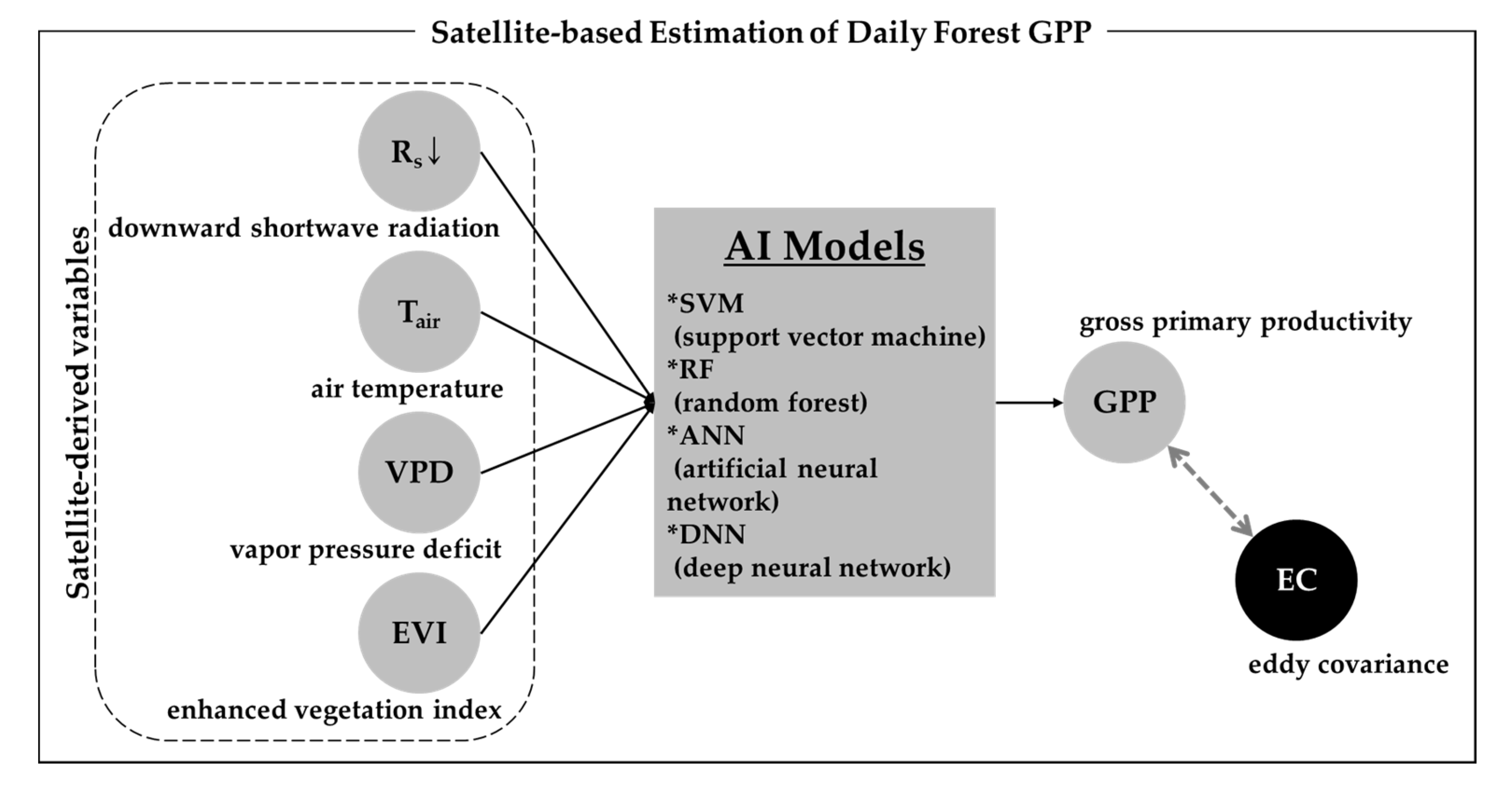
2.3. Artificial Intelligence Models

2.3.1. Support Vector Machine

SVM is a technique for optimal classification, and the support vector regression (SVR) is a regression model for the optimally classified data groups derived from the SVM. For optimal classification, a maximum margin hyperplane (MMH) can be set up by maximizing the margin between data groups using nonlinear kernel functions such as polynomial and Gaussian functions [40]. We used the e1071 library in R and the gaussian radial basis function for the nonlinear MMH. The cost parameter was set to 1 for outlier management, and the gamma parameter was set to 1/n (n is the data dimension) for the definition of a normal distribution.

2.3.2. Random Forest

RF is an ensemble method that utilizes a number of decision trees derived from random samples. If necessary, a bootstrap process is performed for resampling by taking account of the sample distribution. A bagging (bootstrap aggregating) process creates a final solution by averaging the results from the bootstrapped trees [41]. In our experiment, the number of trees was set to 500, and the number of variables used for splitting tree branches was set to n/2 (n is the number of input variables), using the randomForest library in R.

2.3.3. Artificial Neural Network

ANN emulates a biological neural system. It consists of an input layer for explanatory variables, multiple hidden layers for nonlinear computations, and an output layer to produce a result [42,43]. The sets of weight and bias in the neural network are optimized by minimizing a cost function between true labels and estimated values. We carried out the hyperparameter optimization using the nnet library in R, such as 2 for the number of hidden units; 100 for the maximum iteration; Broyden–Fletcher–Goldfarb–Shanno (BFGS) algorithm for the adaptive learning rate [43].

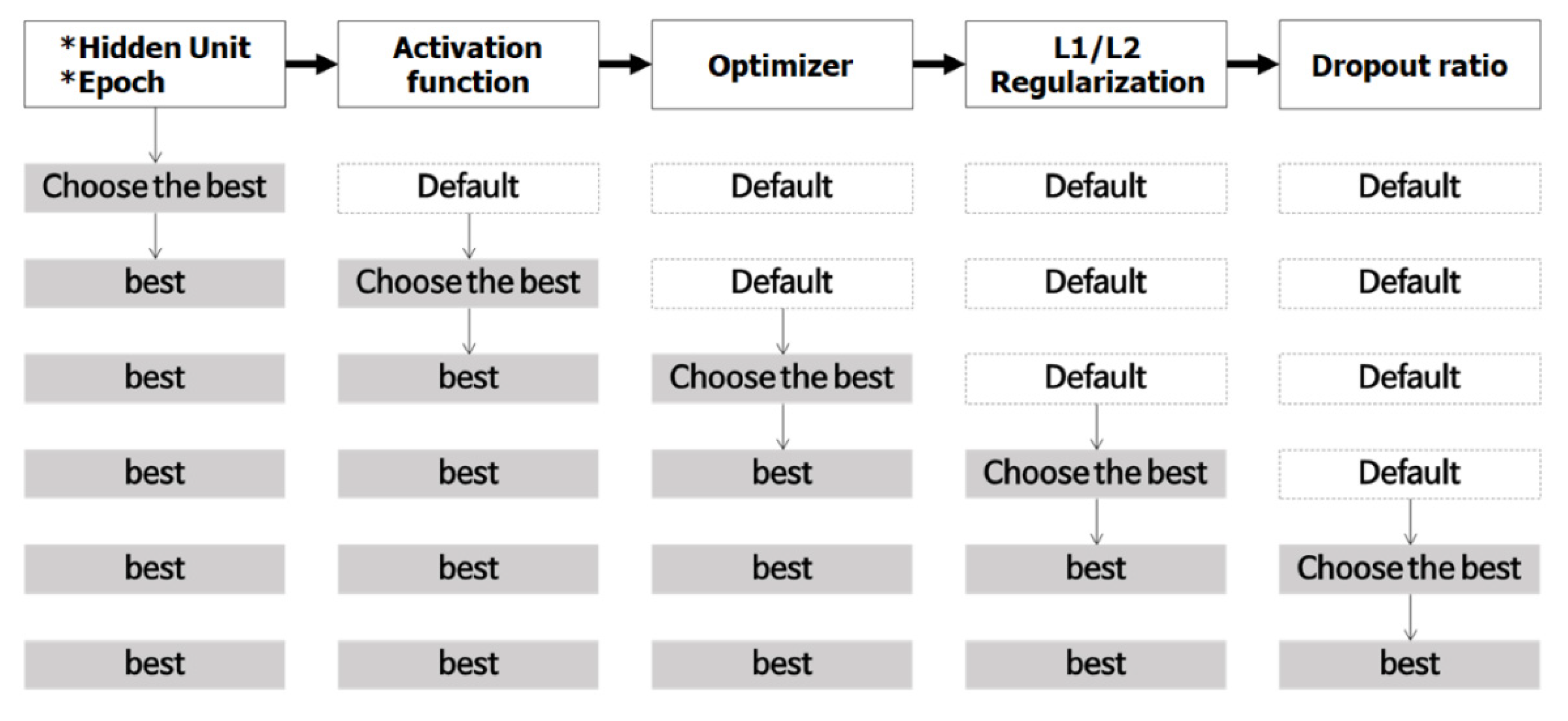
2.3.4. Deep Neural Network

The classic ANN might stop at a locally optimized state, and the generic machine learning might cause an overfitting problem. DNN is a technique developed to mitigate these problems by an intensive optimization in the deep and thick hidden layers in a neural network. The rectified linear units (ReLU) activation function can avoid the vanishing gradient phenomenon during the minimization of a loss function. The regularization can make the weighting scheme of a neural network less biased to a specific neuron, and the dropout methods can cope with unexpected cases in a newly given dataset through a handicapped training with the random elimination of part of the neurons [44]. We adopted the AdaDelta optimizer, which can adjust the learning rate of a neural network adaptively using a dynamic update mechanism and thus can train a DNN model more efficiently and precisely [45]. The configuration process of our DNN model is summarized in Figure 3 [46]. We used the h2o library in R for the hyperparameter optimization, such as 500–500–500 for the hidden unit; 300 for the epoch; ReLU for the activation function; AdaDelta for the optimizer; 20% for the dropout ratio.

2.4. Validations

The daily GPP estimates by the four AI models were validated using the leave-one-year-out (a.k.a. jackknife) method. The calibration was carried out from a 10 year dataset except for one year, and the validation was conducted for the excluded one year. Such cross-validation processes were repeated ten times for each year from 2006 to 2015. Validation statistics such as mean bias error (MBE), mean absolute error (MAE), root mean square error (RMSE), and CC were used.

To compare the performance of the AI predictions with that of the currently operative GPP products, we collected the MODIS and the FluxCom GPP during 2006–2015. MODIS Terra and Aqua products (MOD17A2HGF and MYD17A2HGF) comprise a gap-filled dataset that has less uncertainty than the previous version (MOD17A2 and MYD17A2). The gap-filling process was conducted at the end of each year using a reliable dataset for the fraction of photosynthetically active radiation (FPAR) and LAI [47]. Because these products have a spatial resolution of 500 m and a temporal resolution of 8 days, our daily GPP estimates were aggregated into an 8 day composite for the comparison of performance. For another comparison, we obtained the AI-based FluxCom GPP products with a spatial resolution of 10 km and a temporal resolution of 8 days. However, all the pixels on the Gwangneung site had missing values for the entire period, thus the performance comparison with the FluxCom GPP could not be carried out.

3. Results

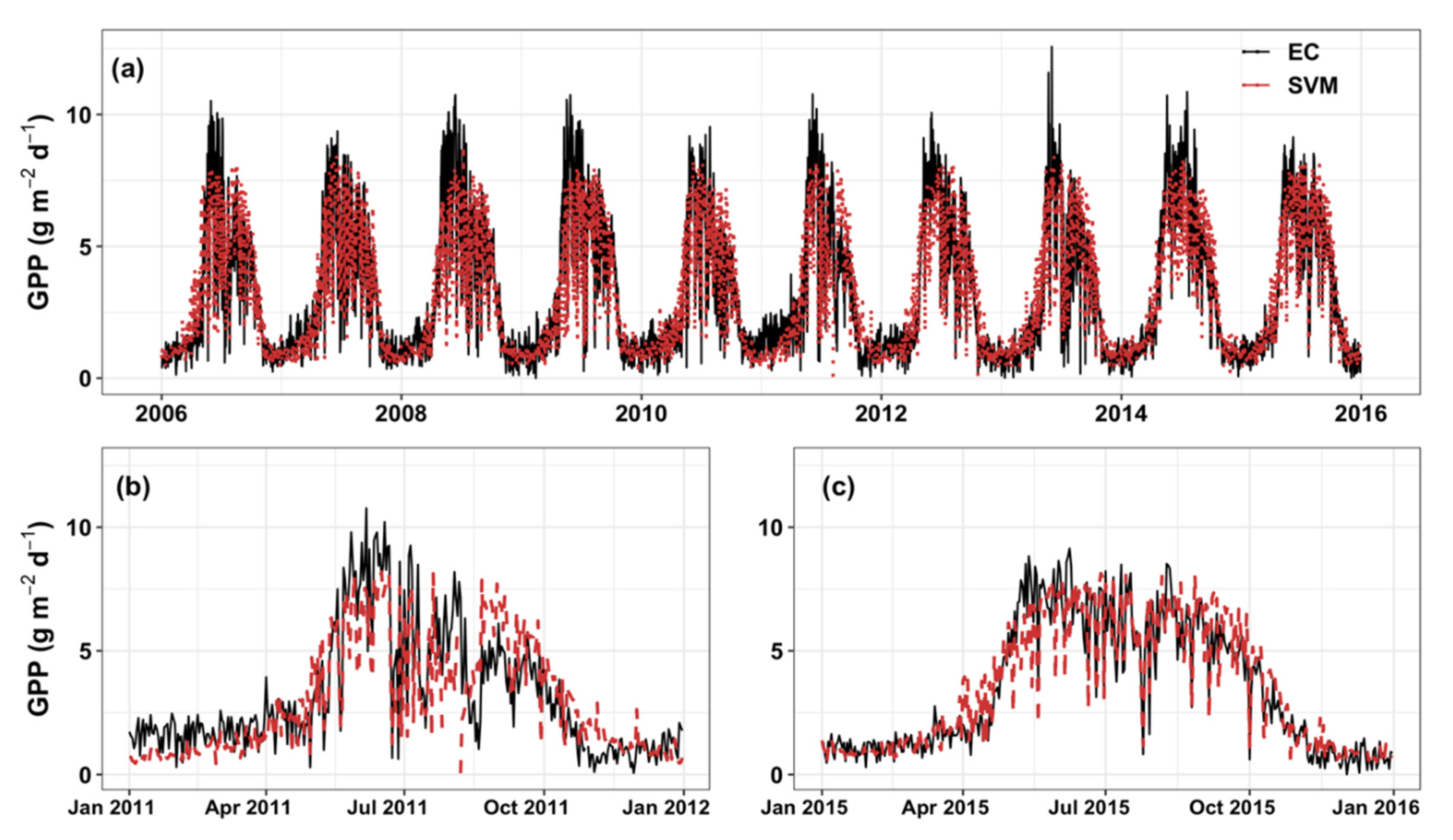
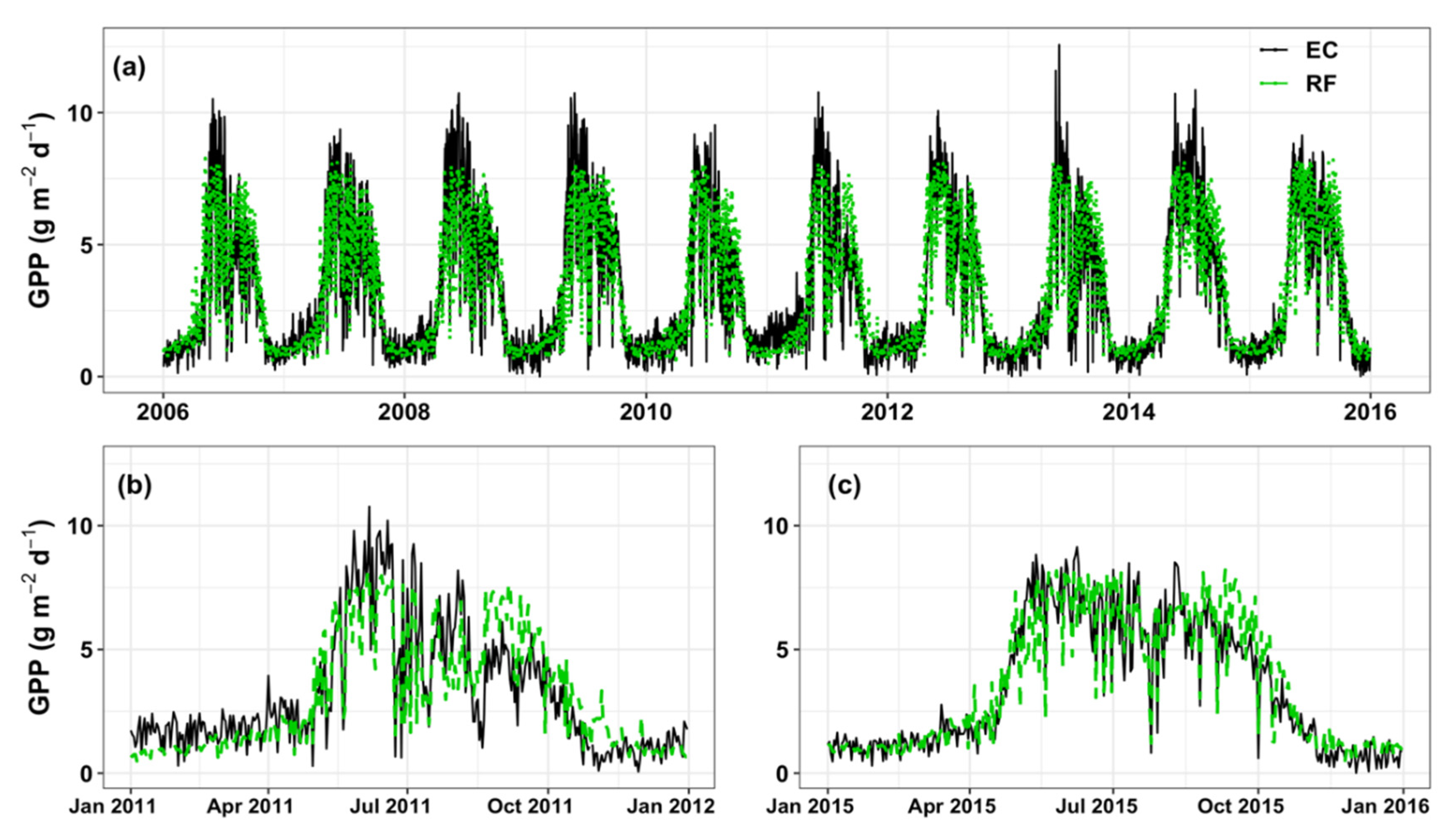
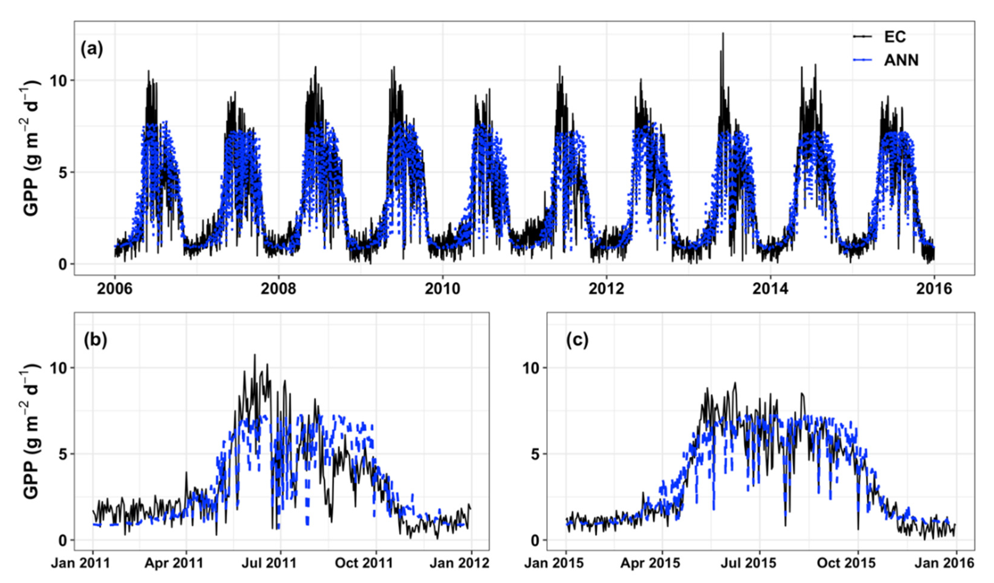
3.1. GPP Estimation by AI Models

Table 2. Statistics of daily gross primary productivity (GPP) at the Gwangneung site for the period between 2006 and 2015, measured by eddy covariance (EC) and predicted by support vector machine (SVM), random forest (RF), artificial neural network (ANN), and deep neural network (DNN).

Method	Min (1) (g m−2 d−1)	Max (2) (g m−2 d−1)	Mean (g m−2 d−1)
EC	0.28	9.20	3.30
SVM	0.58	7.76	3.26
RF	0.74	7.83	3.35
ANN	0.85	7.49	3.35
DNN	0.55	8.49	3.29

⁽¹⁾ Minimum value except for lower 2% data; ⁽²⁾ maximum value except for upper 2% data.

and

Table 3. Statistics of daily gross primary productivity (GPP) at the Gwangneung site for each year between 2006 and 2015, measured by eddy covariance (EC) and predicted by support vector machine (SVM), random forest (RF), artificial neural network (ANN), and deep neural network (DNN).

Year	Method	Min (1) (g m−2 d−1)	Max (2) (g m−2 d−1)	Mean (g m−2 d−1)
2006	EC	0.42	9.68	3.10
	SVM	0.64	7.69	3.27
	RF	0.73	7.70	3.34
	ANN	0.90	7.60	3.37
	DNN	0.74	8.15	3.27
2007	EC	0.44	8.47	3.19
	SVM	0.62	7.97	3.15
	RF	0.76	7.82	3.28
	ANN	0.91	7.22	3.25
	DNN	0.55	7.44	2.82
2008	EC	0.32	9.76	3.65
	SVM	0.65	7.55	3.33
	RF	0.76	7.71	3.40
	ANN	0.74	7.65	3.39
	DNN	1.04	8.85	3.77
2009	EC	0.28	9.66	3.53
	SVM	0.59	7.69	3.25
	RF	0.77	7.81	3.36
	ANN	0.87	7.60	3.28
	DNN	0.34	8.95	3.45
2010	EC	0.41	8.55	2.98
	SVM	0.56	7.74	3.11
	RF	0.71	7.73	3.16
	ANN	0.86	7.60	3.16
	DNN	0.59	8.30	2.95
2011	EC	0.36	9.26	3.14
	SVM	0.47	7.85	2.94
	RF	0.70	7.62	3.10
	ANN	0.85	7.22	3.20
	DNN	1.38	8.57	3.27
2012	EC	0.26	8.51	3.35
	SVM	0.60	7.70	3.24
	RF	0.77	7.83	3.39
	ANN	0.86	7.70	3.39
	DNN	0.32	8.50	3.32
2013	EC	−0.03	8.84	3.05
	SVM	0.58	7.72	3.30
	RF	0.73	7.73	3.29
	ANN	0.83	7.20	3.37
	DNN	0.32	8.49	3.07
2014	EC	0.33	9.35	3.56
	SVM	0.57	7.70	3.43
	RF	0.77	7.89	3.53
	ANN	0.90	7.19	3.49
	DNN	0.65	8.04	3.51
2015	EC	0.25	8.48	3.49
	SVM	0.61	7.84	3.56
	RF	0.73	8.10	3.66
	ANN	0.92	7.22	3.62
	DNN	0.72	7.72	3.45

⁽¹⁾ Minimum value except for lower 2% data; ⁽²⁾ maximum value except for upper 2% data.

show the statistics of the daily GPP at the Gwangneung site between 2006 and 2015, including the predictions from SVM, RF, ANN, and DNN as well as the observations from the EC. The mean values of the predicted GPP by the AI models (3.26–3.35 g m⁻² d⁻¹) were very similar to those of the EC measurements (3.30 g m⁻² d⁻¹). However, the AI models did not well represent very low or very high GPP values, thus the daily GPP under approximately 0.5 g m⁻² d⁻¹ or over about 8.5 g m⁻² d⁻¹ was rarely simulated by the AI models. Among the four AI models, the DNN showed the closest predictions in terms of the minimum, maximum, and mean values.

Figure 4, Figure 5, Figure 6 and Figure 7 show the seasonal changes of the predicted daily GPP at the Gwangneung site for the period between 2006 and 2015. The four AI models closely traced the growing season (increasing phase) and the senescence (decreasing phase) of the forest every year. The curve in spring showed an exponential increment, and that of autumn had a relatively longer decreasing period in both AI and EC GPPs. The DNN model followed the GPP peak in May and June better than SVM, RF, and ANN models (Figure 4a, Figure 5a, Figure 6a and Figure 7a).

Table 4. Validation statistics of daily gross primary productivity (GPP) at the Gwangneung site for the period between 2006 and 2015, predicted by support vector machine (SVM), random forest (RF), artificial neural network (ANN), and deep neural network (DNN).

Model	Year	MBE (1) (g m−2 d−1)	MAE (2) (g m−2 d−1)	RMSE (3) (g m−2 d−1)	CC (4)	Model	Year	MBE (g m−2 d−1)	MAE (g m−2 d−1)	RMSE (g m−2 d−1)	CC
SVM	2006	0.17	0.87	1.24	0.88	RF	2006	0.25	0.80	1.14	0.90
	2007	−0.04	0.75	1.01	0.91		2007	0.09	0.71	0.96	0.92
	2008	−0.31	0.88	1.25	0.91		2008	−0.25	0.81	1.17	0.92
	2009	−0.28	0.78	1.12	0.92		2009	−0.17	0.73	1.04	0.93
	2010	0.13	0.79	1.06	0.90		2010	0.18	0.77	1.08	0.90
	2011	−0.20	1.07	1.45	0.81		2011	−0.04	0.97	1.26	0.86
	2012	−0.11	0.81	1.12	0.91		2012	0.04	0.69	0.97	0.93
	2013	0.26	0.77	1.06	0.92		2013	0.24	0.69	0.96	0.94
	2014	−0.13	0.89	1.24	0.91		2014	−0.03	0.85	1.21	0.91
	2015	0.08	0.68	0.95	0.93		2015	0.17	0.68	0.95	0.94
	Avg.	−0.04	0.83	1.15	0.90		Avg.	0.05	0.77	1.07	0.92
ANN	2006	0.27	0.87	1.24	0.88	DNN	2006	0.18	0.70	1.02	0.92
	2007	0.06	0.79	1.08	0.90		2007	−0.37	0.75	1.03	0.92
	2008	−0.26	0.91	1.23	0.91		2008	0.12	0.71	0.97	0.94
	2009	−0.24	0.77	1.09	0.93		2009	−0.07	0.67	0.95	0.94
	2010	0.18	0.84	1.16	0.88		2010	−0.03	0.67	0.94	0.92
	2011	0.05	1.06	1.39	0.83		2011	0.13	0.77	1.05	0.90
	2012	0.03	0.81	1.11	0.91		2012	−0.03	0.68	0.92	0.94
	2013	0.32	0.82	1.15	0.91		2013	0.02	0.58	0.87	0.94
	2014	−0.07	0.88	1.23	0.91		2014	−0.05	0.66	0.97	0.94
	2015	0.14	0.70	0.96	0.93		2015	−0.04	0.63	0.90	0.94
	Avg.	0.05	0.85	1.16	0.90		Avg.	−0.01	0.68	0.96	0.93

⁽¹⁾ mean bias error; ⁽²⁾ mean absolute error; ⁽³⁾ root mean square error; ⁽⁴⁾ correlation coefficient.

shows the validation statistics of the daily GPP in terms of MBE, MAE, RMSE, and CC. The averages of CC had small differences among the four AI models (between 0.90 and 0.93), but the DNN model demonstrated significantly better accuracy in terms of MAE and RMSE. The MAE was approximately 13% ((0.77−0.68)/0.68) to 25% ((0.85−0.68)/0.68) better, and the RMSE was about 11% ((1.07−0.96)/0.96) to 21% ((1.16−0.96)/0.96) better than the other three models. In the year 2011, South Korea experienced multiple extreme weather events. The four AI models showed the lowest accuracy, with the CC between 0.81 and 0.86 for SVM, RF, and ANN and the CC of 0.90 for the DNN model. A cold wave lasted for almost 40 days from December 2010 to January 2011. Heavy rain for nine consecutive days in June resulted in a large-scale landslide in Seoul. An extraordinarily late heatwave occurred for several days in autumn. Such extreme weather events led to a lower GPP (2.40 g m⁻² d⁻¹) than the usual years (3.30 g m⁻² d⁻¹), thus the GPP predictions using R_s↓, T_air, VPD, and EVI did not perform very well due to the unexpected weather conditions. However, the DNN model showed similar predictability to the usual years despite the extreme weather: the MAE of 0.77 g m⁻² d⁻¹, the RMSE of 1.05 g m⁻² d⁻¹, and the CC of 0.90. Figure 4c, Figure 5c, Figure 6c and Figure 7c show the time series of 2015 when the predictions of the four models were best among all the years. On the other hand, the predictions in 2011 by SVM, RF, and ANN models did not coincide very well with the EC observations (Figure 4b, Figure 5b and Figure 6b), whereas the DNN predictions in 2011 in Figure 7b had relatively good agreements with the EC values. Additionally, the DNN model could simulate very high GPP values over about 8 g m⁻² d⁻¹, while the other three models showed an upward stiffness that could not produce such high values.

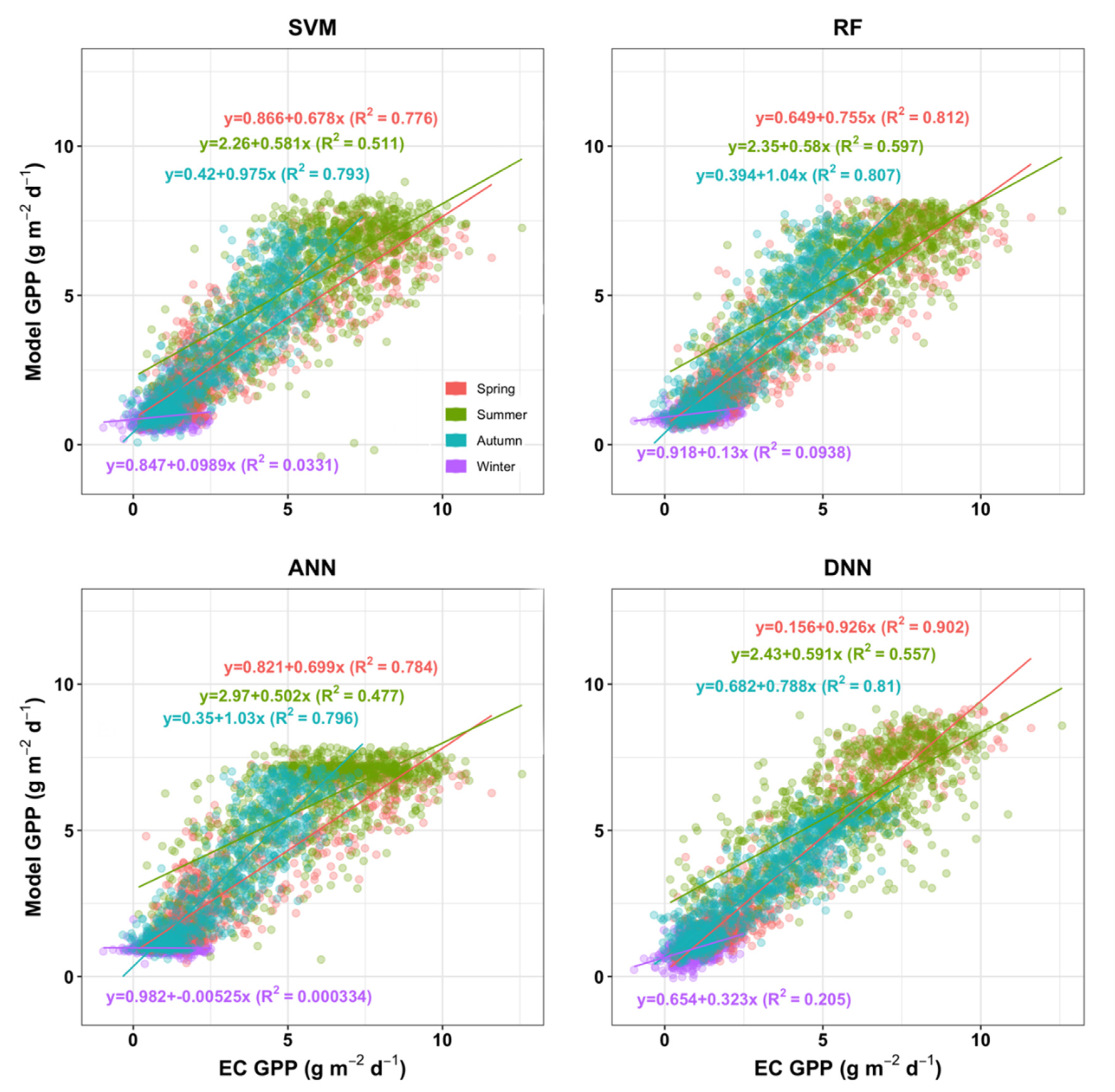
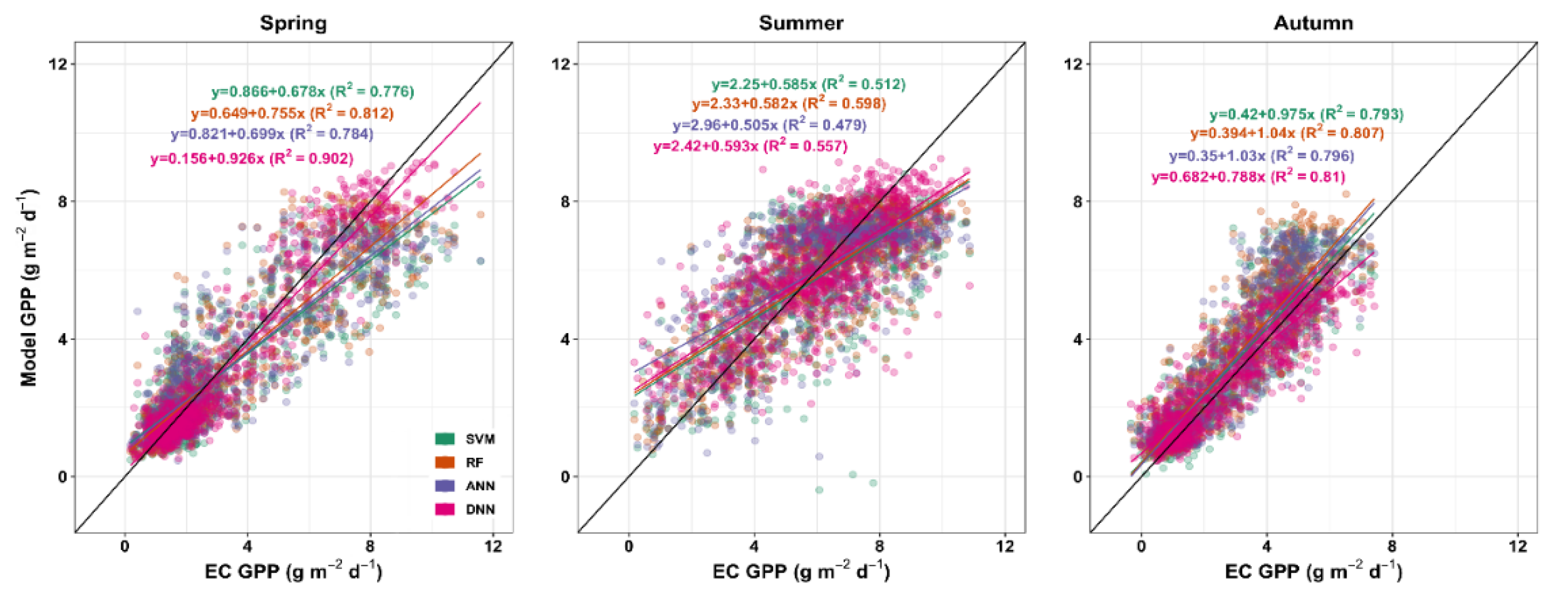
3.2. Seasonal Characteristics of Validation Statistics

We examined the accuracy of daily GPP predictions according to seasons: spring (March, April, and May), summer (June, July, and August), autumn (September, October, and November), and winter (December, January, and February). Figure 8 shows the CC between the observed and the predicted GPP by the four AI models. The CC of spring and autumn was quite high (around 0.9), while that of summer was relatively low (approximately 0.7 to 0.8). The accuracy of winter was worse than other seasons: the CC for SVM, RF, and ANN was around 0 to 0.3, while the CC for DNN was about 0.45 (Figure 8). The CC values in the cold months from November to March were also low. Nevertheless, the DNN model showed an overall concentrated scatterplot along the 1:1 line compared to the other three models that had a tendency of underestimation in spring and summer and a tendency of overestimation in autumn (Figure 9 and Figure 10).

3.3. Comparisons with Operative GPP Products

Table 5. Validation statistics of 8 day gross primary productivity (GPP) at the Gwangneung site from Moderate-resolution Imaging Spectroradiometer (MODIS) products and the deep neural network (DNN) predictions, against the eddy covariance (EC) measurements during 2006–2015.

GPP Data	MBE (g m−2 d−1)	MAE (g m−2 d−1)	RMSE (g m−2 d−1)	CC
DNN	−0.014	0.405	0.537	0.975
MODIS (Terra)	0.224	0.998	1.278	0.916
MODIS (Aqua)	0.119	0.946	1.195	0.915

shows the validation statistics for the 460 cases of the 8 day composite against the EC measurements during 2006–2015. The performances of the three 8 day composites (DNN, Terra, and Aqua) were quite good because of temporal smoothing effects, but the DNN estimates outperformed the Terra and the Aqua products for the Gwangneung site. In terms of the RMSE, our result was 58% better than that of Terra ((1.278−0.537)/1.278) and 55% better than that of Aqua ((1.195−0.537)/1.195). Moreover, the DNN estimates showed an excellent CC of 0.975.

4. Discussions

In this study, we examined the suitability and the potential of AI models for the forest GPP predictions in South Korea. Among the four AI models, DNN showed the best performance in terms of validation statistics and the applicability to unexpected weather conditions. We discussed the performance of the AI models and explored the advantages and the limitations of our experiment.

4.1. Performance of AI Models

The results showed a tendency of strong agreement between the GPPs predicted by the AI models and by the EC measurements, explaining approximately 90% of the temporal changes in daily GPP. The phenology of forest vegetation is primarily divided into growth and senescence phases. The predicted GPP at the start of the growing season (increasing phase of each year) and the end of the growing season (decreasing phase of each year) consistently followed the EC measurements. Understanding the seasonal development on daily GPP and environmental factors such as R_s↓, T_air, VPD, and EVI is critical to the applicability of the nonlinear relationships between the input variables and the GPP predictions. Each phase follows a different phenological development, leading to different relationships between the input variables and the GPP. The AI models consistently demonstrated a reasonable correlation in the estimation of daily GPP (Table 4). Indeed, AI techniques in recent years have been considered a viable option for the retrieval of terrestrial carbon fluxes on a spatially continuous grid. Our experiment also showed the possibility of the AI-based GPP prediction, particularly for the local-scale applications for the countries with complex terrains such as South Korea. The integration of AI techniques with satellite images can be an alternative to studies of the interactions between atmosphere and forest ecosystems. Previous studies showed that the AI applications combined with satellite images were effective for estimation of GPP, above-ground biomass, ecosystem respiration, and latent heat flux [24,25,48,49].

Moreover, a deep learning approach such as DNN in our experiment can be thought of as a better method than the classical AI models such as RF, SVM, and ANN. The DNN presented a superior performance to the other three models in terms of the validation statistics and the representation of seasonal patterns. The overall accuracy decreased in winter because the site is a warm-temperate deciduous forest in which winter photosynthesis is almost inactive. However, the DNN could simulate the winter GPP values much better than the other three AI models. It is because the DNN is a method developed to resolve local minima and overfitting problems of the classical AI models. The DNN model was more optimized in a deep and thick network using the ReLU activation function, the AdaDelta optimizer, and the appropriate outlier management by regularization and dropout techniques. Moreover, we demonstrated that the DNN model performed well despite the multiple extreme weather events such as cold waves, heavy rain, and an autumnal heatwave in 2011 in South Korea. The comparison with MODIS products also showed that our DNN model was locally optimized for the forests in South Korea on a daily basis, while the parameterization of the MODIS GPP was not specifically suitable for South Korea. Such an outcome of the DNN model was partly because of the spatiotemporally appropriate arrangement of the satellite data. The 16 day albedo and the daily EVI interpolated from 8 day data were also suitable for use in the estimation of daily GPP, which is in accordance with previous studies [50,51].

4.2. Limitations and Future Work

We made sure that the AI models such as DNN were very effective in resolving the nonlinear issues for GPP prediction. The DNN model provides a useful method to overcome the limitations of linear and process-based models. However, a limited volume of data can lead to degradation of accuracy since it may not sufficiently represent the various aspects of GPP changes [24,43]. A large database from various locations of EC measurements will be required for a more advanced DNN model. A longer time series to cover various weather events will also be necessary to cope with unexpected outlier cases. By using such big data for GPP prediction, we can produce an alternative GPP map from the improved DNN model. Moreover, a spatially continuous retrieval of forest GPP over South Korea can be achieved after the improved DNN model is combined with a higher-quality dataset. For example, the advanced versions of the MODIS products, such as gap-filled snow-free daily albedo (MCD43GF), gap-filled daily AOD with the multi-angle implementation of atmospheric correction (MAIAC) (MCD19A2), and gap-filled daily surface radiation (MCD18A1), are now available. Additionally, the meteorological reanalysis such as Local Data Assimilation and Prediction System (LDAPS) of South Korea can be used for the local-scale land surface variables such as sensible/latent/soil heat flux, temperature, humidity, wind, and precipitation. The use of meteorological reanalysis will also help avoid the problem of the cloud-covered pixels in satellite images.

5. Conclusions

Many process-based models for carbon flux predictions have faced a wide range of uncertainty issues in the model result. The complex interactions between atmosphere and forest ecosystems are the main reason for the uncertainty. However, the setting of too many initial parameters might lead to disturbing accuracy improvement. On the other hand, artificial intelligence techniques, which are novel methods to resolve complex and nonlinear problems, have shown a possibility for forest ecological applications. This study is the first step to present an objective comparison between multiple AI models for the daily forest GPP prediction using satellite remote sensing data. In particular, the DNN model outperformed the other three models through an intensive hyperparameter optimization in a deep learning network. We showed that the DNN model also performed well under conditions of cold waves, heavy rain, and an autumnal heatwave. In the experiment, our DNN model showed better accuracy than the operative MODIS GPP product, presumably because of the localized optimization for the forests in South Korea. A spatially continuous retrieval of forest GPP can be achieved after the integration of more improved DNN models and higher-quality datasets from satellite remote sensing and meteorological reanalysis. As future work, a comprehensive comparison with the result of process-based models will be necessary using a more extensive EC database from various forest ecosystems. Such comparisons can produce a synergy between the process-based models that have advantages for the understanding of the mechanism and the AI models that have the ability to solve nonlinear problems. In this sense, more efforts for the AI-based modeling of forest GPP will also be required.

References

1. FAOSTAT. Statistical Database of the Food and Agriculture Organization of the United Nations. Available online: http://faostat.fao.org/ (accessed on 31 August 2020).
2. Stephenson, N.L.; Das, A.J.; Condit, R.; Russo, S.E.; Baker, P.J.; Beckman, N.G.; Coomes, D.A.; Lines, E.R.; Morris, W.K.; Ruger, N.; et al. Rate of tree carbon accumulation increases continuously with tree size. Nature 2014, 507, 90–93. [Google Scholar] [CrossRef]
3. Running, S.W.; Baldocchi, D.D.; Turner, D.P.; Gower, S.T.; Bakwin, P.S.; Hibbard, K.A. A global terrestrial monitoring network integrating tower fluxes, flask sampling, ecosystem modeling and EOS satellite data. Remote Sens. Environ. 1999, 70, 108–127. [Google Scholar] [CrossRef]
4. Smith, P.; Lanigan, G.; Kutsch, W.L.; Buchmann, N.; Eugster, W.; Aubinet, M.; Ceschia, E.; Béziat, P.; Yeluripati, J.B.; Osborne, B.; et al. Measurements necessary for assessing the net ecosystem carbon budget of croplands. Agric. Ecosyst. Environ. 2010, 139, 302–315. [Google Scholar] [CrossRef]
5. Ogutu, B.O.; Dash, J.; Dawson, T.P. Developing a diagnostic model for estimating terrestrial vegetation gross primary productivity using the photosynthetic quantum yield and Earth Observation data. Glob. Chang. Biol. 2013, 19, 2878–2892. [Google Scholar] [CrossRef] [PubMed]
6. Farquhar, G.D.; Sharkey, T.D. Stomatal conductance and photosynthesis. Ann. Rev. Plant Physiol. 1982, 33, 317–345. [Google Scholar] [CrossRef]
7. Schulze, E.D. Biological control of the terrestrial carbon sink. Biogeosciences 2006, 3, 147–166. [Google Scholar] [CrossRef] [Green Version]
8. Kang, M.; Kim, J.; Kim, H.S.; Thakuri, B.M.; Chun, J.H. On the nighttime correction of CO2 flux measured by eddy covariance over temperate forests in complex terrain. Korean J. Agric. For. Meteorol. 2014, 16, 233–245, (In Korean with English abstract). [Google Scholar] [CrossRef] [Green Version]
9. Baldocchi, D.; Falge, E.; Gu, L.; Olson, R.; Hollinger, D.; Running, S.; Anthoni, P.; Bernhofer, C.; Davis, K.; Evans, R.; et al. FLUXNET: A new tool to study the temporal and spatial variability of ecosystem-scale carbon dioxide, water vapor, and energy flux densities. Bull. Am. Meteorol. Soc. 2001, 82, 2415–2434. [Google Scholar] [CrossRef]
10. Xiao, X.; Zhang, Q.; Braswell, B.; Urbanski, S.; Boles, S.; Wofsy, S.; Moore, B., III; Ojima, D. Modeling gross primary production of temperate deciduous broadleaf forest using satellite images and climate data. Remote Sens. Environ. 2004, 91, 256–270. [Google Scholar] [CrossRef]
11. Baldocchi, D.D. Assessing the eddy covariance technique for evaluating carbon dioxide exchange rates of ecosystems: Past, present and future. Glob. Chang. Biol. 2003, 9, 479–492. [Google Scholar] [CrossRef] [Green Version]
12. Reeves, M.C.; Zhao, M.; Running, S.W. Usefulness and limits of MODIS GPP for estimating wheat yield. Int. J. Remote Sens. 2007, 26, 1403–1421. [Google Scholar] [CrossRef]
13. Tenhunen, J.D.; Yocum, C.S.; Gates, D.M. Development of a photosynthesis model with an emphasis on ecological applications. Oecologia 1976, 26, 89–100. [Google Scholar] [CrossRef]
14. Falge, E.; Graber, W.; Siegwolf, R.; Tenhunen, J.D. A model of the gas exchange response of Picea abies to habitat conditions. Trees 1996, 10, 277–287. [Google Scholar]
15. Muraoka, H.; Koizumi, H. Photosynthetic and structural characteristics of canopy and shrub trees in a cool-temperate deciduous broadleaved forest: Implication to the ecosystem carbon gain. Agric. Ecosyst. Environ. 2005, 134, 39–59. [Google Scholar] [CrossRef]
16. Schindler, D.E.; Hilborn, R. Prediction, precaution, and policy under global change. Science 2015, 347, 953–954. [Google Scholar] [CrossRef] [PubMed] [Green Version]
17. Ye, H.; Beamish, R.J.; Glaser, S.M.; Grant, S.C.H.; Hsieh, C.H.; Richards, L.J.; Schnute, J.T.; Sugihara, G. Equation-free mechanistic ecosystem forecasting using empirical dynamic modeling. Proc. Natl. Acad. Sci. USA 2015, 112, E1569–E1576. [Google Scholar] [CrossRef] [PubMed] [Green Version]
18. Dou, X.; Yang, Y.; Luo, J. Estimating forest carbon fluxes using machine learning techniques based on Eddy covariance measurements. Sustainability 2018, 10, 203. [Google Scholar] [CrossRef] [Green Version]
19. Stockwell, D.; Modelling, A.P.E. Effects of sample size on accuracy of species distribution models. Ecol. Model. 2002, 148, 1–13. [Google Scholar] [CrossRef]
20. Elith, J.; Leathwick, J.R. Species distribution models: Ecological explanation and prediction across space and time. Annu. Rev. Ecol. Evol. Syst. 2009, 40, 415–436. [Google Scholar] [CrossRef]
21. Kim, N.S.; Han, D.; Cha, J.Y.; Park, Y.S.; Cho, H.J.; Kwon, H.J.; Cho, Y.C.; Oh, S.H.; Lee, C.S. A detection of novel habitats of Abies koreana by using species distribution models (SDMs) and its application for plant conservation. J. Korea Soc. Environ. Restor. Technol. 2015, 18, 135–149. [Google Scholar] [CrossRef] [Green Version]
22. Marrs, J.; Ni-Meister, W. Machine learning techniques for tree species classification using co-registered LiDAR and hyperspectral data. Remote Sens. 2019, 11, 819. [Google Scholar] [CrossRef] [Green Version]
23. Tramontana, G.; Ichii, K.; Camps-Valls, G.; Tomelleri, E.; Papale, D. Uncertainty analysis of gross primary production upscaling using random forests, remote sensing and eddy covariance data. Remote Sens. Environ. 2015, 168, 360–373. [Google Scholar] [CrossRef]
24. Ichii, K.; Ueyama, M.; Kondo, M.; Saigusa, N.; Kim, J.; Alberto, M.C.; Ardö, J.; Euskirchen, E.S.; Kang, M.; Hirano, T.; et al. New data-driven estimation of terrestrial CO2 fluxes in Asia using a standardized database of eddy covariance measurements, remote sensing data, and support vector regression. J. Geophys. Res. Biogeosci. 2017, 122, 767–795. [Google Scholar] [CrossRef]
25. Wang, X.; Yao, Y.; Zhao, S.; Jia, K.; Zhang, X.; Zhang, Y.; Zhang, L.; Xu, J.; Chen, X. MODIS-based estimation of terrestrial latent heat flux over North America using three machine learning algorithms. Remote Sens. 2017, 9, 1326. [Google Scholar] [CrossRef] [Green Version]
26. Kim, J.; Lee, D.; Hong, J.; Kang, S.; Kim, S.J.; Moon, S.K.; Lim, J.H.; Son, Y.; Lee, J.; Kim, S.; et al. HydroKorea and CarboKorea: Cross-scale studies of ecohydrology and biogeochemistry in a heterogeneous and complex forest catchment of Korea. Ecol. Res. 2006, 21, 881–889. [Google Scholar] [CrossRef]
27. Kwon, H.; Kim, J.; Hong, J.; Lim, J.H. Influence of the Asian monsoon on net ecosystem carbon exchange in two major ecosystems in Korea. Biogeosciences 2010, 7, 1493–1504. [Google Scholar] [CrossRef] [Green Version]
28. Hong, J.; Kwon, H.; Lim, J.; Byun, Y.; Lee, J.; Kim, J. Standardization of KoFlux eddy covariance data processing. KJAFM 2009, 11, 19–26, (In Korean with English abstract). [Google Scholar]
29. Kang, M.; Ruddell, B.L.; Cho, C.; Chun, J.; Kim, J. Identifying CO2 advection on a hill slope using information flow. Agric. For. Meteorol. 2017, 232, 265–278. [Google Scholar] [CrossRef] [Green Version]
30. Bisht, G.; Venturini, V.; Islam, S.; Jiang, L. Estimation of the net radiation using MODIS (Moderate Resolution Imaging Spectroradiometer) data for clear sky days. Remote Sens. Environ. 2005, 97, 52–67. [Google Scholar] [CrossRef]
31. Hwang, T.; Kang, S.; Kim, J.; Kim, Y.; Lee, D.; Band, L. Evaluating drought effect on MODIS Gross Primary Production (GPP) with an eco-hydrological model in the mountainous forest, East Asia. Glob. Chang. Biol. 2008, 14, 1037–1056. [Google Scholar] [CrossRef]
32. Bird, R.E.; Hulstrom, R.L. A Simplified Clear Sky Model for Direct and Diffuse Insolation on Horizontal Surfaces; SERI Technical Report SERI/TR-642-761; Solar Energy Research Institute: Golden, CO, USA, 1981. [Google Scholar] [CrossRef] [Green Version]
33. Ryu, Y.; Kang, S.; Moon, S.-K.; Kim, J. Evaluation of land surface radiation balance derived from moderate resolution imaging spectroradiometer (MODIS) over complex terrain and heterogeneous landscape on clear sky days. Agric. For. Meteorol. 2008, 148, 1538–1552. [Google Scholar] [CrossRef]
34. Kang, S.; Running, S.W.; Zhao, M.; Kimball, J.S.; Glassy, J. Improving continuity of MODIS terrestrial photosynthesis products using an interpolation scheme for cloudy pixels. Int. J. Remote Sens. 2005, 26, 1659–1676. [Google Scholar] [CrossRef]
35. Jang, K.; Kang, S.K.; Kim, H.W.; Kwon, H.J. Evaluation of shortwave irradiance and evapotranspiration derived from Moderate Resolution Imaging Spectroradiometer (MODIS). Asia Pac. J. Atmos. Sci. 2009, 45, 233–246. [Google Scholar]
36. Jang, K.; Kang, S.; Kim, J.; Lee, C.B.; Kim, T.; Kim, J.; Hirata, R.; Saigusa, N. Mapping evapotranspiration using MODIS and MM5 four-dimensional data assimilation. Remote Sens. Environ. 2010, 114, 657–673. [Google Scholar] [CrossRef]
37. Huete, A.; Didan, K.; Miura, T.; Rodriguez, E.P.; Gao, X.; Ferreira, L.G. Overview of the radiometric and biophysical performance of the MODIS vegetation indices. Remote Sens. Environ. 2002, 83, 195–213. [Google Scholar] [CrossRef]
38. Wardlow, B.D.; Egbert, S.L. A comparison of MODIS 250-m EVI and NDVI data for crop mapping: A case study for southwest Kansas. Int. J. Remote Sens. 2010, 31, 805–830. [Google Scholar] [CrossRef]
39. Lee, B.; Kim, E.; Lim, J.H.; Kang, M.; Kim, J. Application of machine learning algorithm and remote-sensed data to estimate forest pross primary production at multi-sites level. Korean J. Remote Sens. 2019, 35, 1117–1132, (In Korean with English abstract). [Google Scholar]
40. Mountrakis, G.; Im, J.; Ogole, C. Support vector machines in remote sensing: A review. ISPRS J. Photogramm. Remote Sens. 2011, 66, 247–259. [Google Scholar] [CrossRef]
41. Ali, J.; Khan, R.; Ahmad, N.; Maqsood, I. Random forests and decision trees. Int. J. Comput. Sci. Issues 2012, 9, 272–278. [Google Scholar]
42. Lek, S.; Delacoste, M.; Baran, P.; Dimopoulos, I.; Ecological, J.L. Application of neural networks to modelling nonlinear relationships in ecology. Ecol. Model. 1996, 90, 39–52. [Google Scholar] [CrossRef]
43. Kelley, C.T. Iterative Methods for Optimization; Society for Industrial and Applied Mathematics: Philadelphia, PA, USA, 1999. [Google Scholar]
44. Pham, V.; Bluche, T.; Kernorvant, C.; Louradour, J. Dropout improves recurrent neural networks for handwriting recognition. In Proceedings of the 14th International Conference on Frontiers in Handwriting Recognition (ICFHR), Crete, Greece, 1–4 September 2014. [Google Scholar]
45. Zeiler, M.D. AdaDelta: An Adaptive Learning Rate Method. Available online: https://arxiv.org/abs/1212.5701v1 (accessed on 31 August 2020).
46. Kim, N.; Na, S.; Park, C.; Huh, M.; Oh, J.; Ha, K.; Cho, J.; Lee, Y. An artificial intelligence approach to prediction of corn yields under extreme weather conditions using satellite and meteorological data. Appl. Sci. 2020, 10, 3785. [Google Scholar] [CrossRef]
47. NASA. MODIS/Terra Gross Primary Productivity Gap-Filled 8-Day L4 Global 500m SIN Grid V006. Available online: https://ladsweb.modaps.eosdis.nasa.gov/filespec/MODIS/6/MOD17A2HGF (accessed on 31 August 2020).
48. Yang, F.; Ichii, K.; White, M.A.; Hashimoto, H.; Michaelis, A.R.; Votava, P.; Zhu, A.X.; Huete, A.; Running, S.W.; Nemani, R.R. Developing a continental-scale measure of gross primary production by combining MODIS and AmeriFlux data through support vector machine approach. Remote Sens. Environ. 2007, 110, 109–122. [Google Scholar] [CrossRef]
49. Tramontana, G.; Jung, M.; Camps-Valls, G.; Ichii, K.; Ráduly, B.; Reichstein, M.; Schwalm, C.R.; Arain, M.A.; Cescatti, A.; Kiely, G.; et al. Predicting carbon dioxide and energy fluxes across global FLUXNET sites with regression algorithms. Biogeosci. Discuss 2016, 13, 4291–4313. [Google Scholar] [CrossRef] [Green Version]
50. Hmimina, G.; Dufrêne, E.; Pontailler, J.Y.; Delpierre, N.; Aubinet, M.; Caquet, B.; de Grandcourt, A.; Burban, B.; Flechard, C.; Granier, A.; et al. Evaluation of the potential of MODIS satellite data to predict vegetation phenology in different biomes: An investigation using ground-based NDVI measurements. Remote Sens. Environ. 2013, 132, 145–158. [Google Scholar] [CrossRef]
51. Cai, Z.; Jonsson, P.; Jin, H.; Eklundh, L. Performance of smoothing methods for reconstructing NDVI time-series and estimating vegetation phenology from MODIS data. Remote Sens. 2017, 9, 1271. [Google Scholar] [CrossRef] [Green Version]
Figure 1. Gwangneung KoFlux supersite: the location in South Korea (a), a zoomed-in map with its watershed (b), and a photo of the flux tower (c).
Forests 11 01000 g001
Figure 2. Summary of the data used in this study. Input variables were the satellite data such as downward shortwave radiation (Rs↓), air temperature (Tair), vapor pressure deficit (VPD), and enhanced vegetation index (EVI). Gross primary productivity (GPP), the output value, was adjusted using the in-situ observations from the eddy covariance (EC) flux tower.
Forests 11 01000 g002
Figure 3. The parameter optimization process for a deep neural network (DNN) model in this study, which was adopted from [46]. L1—regularization uses the Manhattan norm; L2—regularization uses the Euclidean norm, for the adjustment of weights.
Forests 11 01000 g003
Figure 4. Daily gross primary productivity (GPP) observed by the eddy covariance (EC) method and predicted by a support vector machine (SVM) model at the Gwangneung site during 2006–2015 (a), and the predictions zoomed-in for 2011 (b) and 2015 (c).
Forests 11 01000 g004
Figure 5. Observed vs. predicted daily gross primary productivity (GPP) by a random forest (RF) model at the Gwangneung site during 2006–2015 (a), and the predictions zoomed-in for 2011 (b) and 2015 (c).
Forests 11 01000 g005
Figure 6. Observed vs. predicted daily gross primary productivity (GPP) by an artificial neural network (ANN) model at the Gwangneung site during 2006–2015 (a), and the predictions zoomed-in for 2011 (b) and 2015 (c).
Forests 11 01000 g006
Figure 7. Observed vs. predicted daily gross primary productivity (GPP) by a deep neural network (DNN) model at the Gwangneung site during 2006–2015 (a), and the predictions zoomed-in for 2011 (b) and 2015 (c).
Forests 11 01000 g007
Figure 8. Comparisons of the correlation coefficients between observed vs. predicted gross primary productivity (GPP) by the artificial intelligence (AI) models, according to season (a) and month (b).
Forests 11 01000 g008
Figure 9. Comparisons between artificial intelligence (AI) models for observed vs. predicted gross primary productivity (GPP) by season.
Forests 11 01000 g009
Figure 10. Comparisons between spring, summer, and autumn for the gross primary productivity (GPP) observed vs. predicted by artificial intelligence (AI) models.
Forests 11 01000 g010