Optimal Planning of Wood Harvesting and Timber Supply in Russian Conditions

Abstract

This paper describes an approach to the optimal planning of wood harvesting and timber supply for forest companies of Russia. Software and tools successfully used in other countries (e.g., Finland, Sweden, Canada, etc.) are not as effective in Russian conditions for a number of reasons. This calls for the development of an original approach to solve this problem with respect to Russia’s specific conditions. The main factors affecting the operation of wood harvesting companies in Russia were determined. The optimization problem was formulated taking into account all important features of wood harvesting specific to the country. The mathematical model of the problem was formulated and analyzed. An important requirement is that the solution algorithm should find high-quality plans within short computation times. The original problem was reduced to a block linear programming problem of large dimension, for which an effective numerical solution method was proposed. It is based on the multiplicative simplex method with column generation within Dantzig–Wolfe decomposition and uses heuristics to determine feasible solutions based on the branch and bound method. We tested the solution approach on real production data from a forest company in southern Karelia with a planning horizon up to a year. This case study involved 198 sites and 14 machines harvesting up to 200,000 cubic meters from an available stock volume of about 300,000 cubic meters. An increase in profit by 5% to 10% was observed, measured as revenue from the sale of products, net of harvesting and transportation costs.

1. Introduction

Currently, the active use of decision support systems based on mathematical modeling and operations research, along with geographical information systems (GIS), is considered the most effective way to increase production efficiency in the wood harvesting industry [1]. This approach minimizes the harvesting and transporting costs and leads to higher profits, and also improves other production and economic indicators without additional capital costs. Also, a new promising direction for better forest management focused on information and supporting economic, environmental, and sustainable decisions by using high technology sensing and analytical/digital tools, is the precision forestry. A detailed review of the contribution of the GIS, global navigation satellite systems (GNSS), and various kinds of sensors to forest operation can be found in [2].

Wood harvesting and timber transportation in Russia are typically conducted by wood-harvesting companies operating in leased forests. Forest companies have the opportunity to lease free forest areas from the state for up to 40 years, with possible further extension of the lease, subject to all the rules and norms of sustainable forest management. Forest areas are leased on a competitive basis. Preference is given to companies that have all the necessary resources to conduct business and have proven themselves to be responsible forest users during previous periods. If multiple or gross violations of the principles of sustainable forest management are identified, the lease term may be terminated prematurely.

The supply chain with fully mechanized cut-to-length (CTL) harvesting is used most often. The assortments produced are classified according to their future use, with main groups being sawlogs, pulpwood, energy logs, and logging byproducts. Each group is divided into several subgroups according to their species, qualities, and dimensions. Sawlogs, pulpwood, and energy logs after harvesting are transported by truck or railroad either directly to mills or to intermediate storage areas. The remaining logging residue can be used for the production of bioenergy.

Wood harvesting in natural stands highly limits the possibility of changing the production volume of particular kinds of products (assortments), as their volume distribution varies according to the harvesting site. Thus, finding consumers for all kinds of harvested products is a challenge. The daily changes in the production spatial structure, natural and production conditions, and consumer demand and other factors necessitate an effective decision support tool for wood harvesting planning.

To date, many works have been published that describe approaches to solving various problems related to the optimal planning of wood harvesting [1,2,3,4,5,6,7,8,9,10,11,12,13,14,15]. The majority of these approaches are based on operations research, because corresponding methods, algorithms, and procedures, when used correctly, can yield notable economic and social effects.

An overview and comparison of many works related to planning problems and solution methods can be found in [1]. Early stages were characterized by the use of linear programming (LP) models in forestry planning. In those models, forest management was accounted for in constraints [15], but spatial constraints have not yet been considered. However, such tasks in real production conditions have a very large dimension to be solved using the standard simplex method, because with CTL harvesting on hundreds of sites, dozens of product types are produced, and each is assigned to a specific consumer, the number of which is also measured in the dozens.

A model for harvesting plan optimization with seasonal storage and road network deployment over a 2- to 3-year planning horizon was presented in [3]. In that study, the mixed-integer programming (MIP) problem was solved by strengthening the formulation and using Lagrangean relaxation.

It should be noted that planning of wood harvesting cannot be separated from planning of transportation and road maintenance. A MIP model to solve this multi-element planning problem was proposed by Karlsson et al. [8].

Another important challenge is integrating trucks and other modes of transportation, specifically ships and trains. The development of a new decision support system for transportation planning in Swedish forestry is reported in [7].

Some models were developed to support forest planning taking into account only consumer demand volume, but not prices, harvesting, transportation, and costs [12].

Some authors proposed an optimization model that integrates the assignment of machines to harvest areas and schedules the harvest areas during the year for each machine. The assignment problem is solved in phase 1 and the scheduling problem is solved in phase 2 [4,9].

Nevertheless, in Russia, computer-based decision support tools that automate wood harvesting planning are still used rather seldom. Software and tools successfully used in other countries (e.g., Finland, Sweden, Canada, etc.) [1,2,3,4,5,6,7,8] are not so effective under Russian conditions for a number of reasons, including significant differences in legislation and rules governing wood harvesting due to the state ownership of forest lands, the prevalence of natural untreated mixed stands, the uneven distribution of logging operations throughout the year due to seasonal availability of forest areas, own standards for round wood, different categories and generally poor condition of roads, specific organizational structure of wood-harvesting companies, the mixture of different technologies and machinery, etc. [16,17]. The aim of the research described in this paper is to develop an approach to solve the first and one of the most difficult planning problems of a forestry company—the optimal planning of wood harvesting and timber supply, subject to aforementioned legislative and technological conditions and limitations specific for Russian forestry companies.

The paper is organized as follows. We describe the mathematical model and solution algorithm in Section 2. Section 3 contains numerical results of a case study. Section 4 considers some disadvantages of the approach. Section 5 concludes the paper.

2. Materials and Methods

The following main factors affect the operation of wood harvesting companies in Russia [18,19,20,21]:

1. Annual allowable cut (AAC): the annual volume of timber harvested in a leased forest area. Exceeding the AAC is strictly prohibited. It is regulated by state forestry authorities to ensure sustainable forest management; the volume of harvested wood should not exceed the estimated volume of the annual increase in the leased area. The AAC is assigned separately for production and protective forests, for coniferous and deciduous sites, for main and intermediate forest use, etc. All wood-harvesting companies strive to use the AAC to the maximum extent as far as their specific operational conditions allow.

2. The varying demand for wood harvesting products (assortments) in the operation locality: for example, demand for high-quality roundwood is generally higher than for low-quality firewood, etc. The current forest structure in Russia (natural mixed forests), in which wood-harvesting companies operate, quite often does not match the structure of customer demand. Thus, within the total supply volume there may be a shortage of some assortments and overproduction of others.

3. Accessibility of harvesting sites. One of the most serious problems of wood harvesting in Russia is the poor development of the forest road network; the average length of forest roads in the Russian Federation is 1.46 km per 1000 hectares, whereas in Western Europe and North America it ranges from 10 to 45 km. As the transporting cost accounts for a significant share of wood harvesting operation costs, it forces companies to determine the maximum distance from roundwood customers within which harvesting is economically feasible. For sites located beyond this distance, harvesting is unprofitable. If a new road must be constructed to access a harvesting site, its construction cost further reduces the cost-effective distance. Thus, forest areas that better match the demand structure may be economically unattractive.

4. Production facilities: the machinery, equipment, and labor employed by a wood harvesting company. They can be internal or external (hired).

Thus, to solve the problem of optimal planning of wood harvesting and timber supply on leased forest area, it is necessary to (1) determine the set of sites to be harvested and periods of harvesting on each one within the AAC and use available production facilities; and (2) determine, for each site in the plan, the composition of produced assortments and associate each cubic meter of each assortment to a customer to maximize profit.

At a tactical level, the typical planning horizon is 1 year. The solution to the problem requires such information as purchase prices for different types of assortments for different customers, harvesting and transporting costs, transporting distance, the accessibility of specific harvesting sites during the planning period, required cutting cycles, and the need for new road construction, among others.

More specifically, the main initial data for solving the problem include:

• A list of harvesting sites with locations, including connections to the road network, and necessary details for calculating the output volume of various assortments. From these sites, the algorithm will select the most profitable for harvesting, ceteris paribus.
• Consumer orders including the assortment type, delivery time, and price.
• Production facilities that may be involved in wood harvesting and transportation, including all necessary details, the main being productivity, cost, and location.
• Various technological limitations: AAC, required cutting cycles, machinery productivity, existing road network, seasonal accessibility of harvesting sites, road closing dates, etc.

The initial data may be redundant, which is desirable for the problem solution quality. If the total volume of wood in a harvesting site equals AAC, the task will only be able to determine the harvesting periods and transportation routes. If the number of sites is greater, it enables choosing the most suitable ones. The situation is the same with orders and production facilities: if there is a choice, the plan will include orders and production facilities that result in maximal overall operational efficiency.

The main parameters of objects involved in the task are as follows:

• Planning parameters
  • The planning period (start and end dates)
  • The minimal period from clear-cutting the site (infrastructure cutting before road construction) to putting the road into operation (in days)
• Parameters related to harvesting sites
  • The planned output of various assortments without specified length, calculated using the stock distribution by species and stand value class
  • The felling method (clear-cutting, selective cutting, infrastructure cutting, thinning, etc.)
  • Allowed operation periods (start and end dates), e.g., winter-only sites
  • The earliest possible harvesting start date, if the site is adjacent to another site
  • The obligatory indicator (0/1) that the site must be included in the plan (for whatever reason)
  • Total operation cost, including harvesting, allotment, and road construction, taking into account the location of sand quarries
  • The location on the road network map (latitude and longitude)
• Parameters of lease contracts
  • AAC (in cubic meters)
  • The maximum harvesting volume according to AAC separated by forest category (production, protective), felling method, and species (coniferous, deciduous)
• Parameters of intermediate storage
  • Maximum capacity (in cubic meters)
  • Closing date
  • Location on the road network map (latitude and longitude)
• Parameters of consumer orders
  • Assortment with specific length (in cubic meters)
  • Required volume (in cubic meters)
  • Delivery period (start and end dates)
  • Order priority (integer) reflecting the importance of matching the volume in the order, determined based on the customer rating, and typically highest for contracted orders
  • Demand point on the road network map (latitude and longitude)
• Parameters of wood harvesting machinery
  • Maximum harvesting volume for each felling method within the planning period (in cubic meters)
  • Productivity (in cubic meters per hour)
  • Number of working hours per day and working days per week
• Transporting costs (tariffs)
  • Allowed minimum and maximum transporting distances (in km)
  • Transporting costs for each assortment for specified distance
• Road network, determined by the graph G = <V, E>, where E is the set of road segments and V is the set of map points, and:
  • Each road segment is characterized by the maximum speed, closing periods (e.g., wintertime roads), and operation start date.
  • Map points may be garages, harvesting sites, intermediate storage areas, demand points, terminals, etc.
  • The accessibility, minimum travel time, and minimum distance between map points during a certain period of time are calculated from graph G.

The goal is to find a set of sites the harvesting of which will yield the volume of wood matching customer orders by volume and structure, with the following optimization criteria and constraints.

Optimization criteria

• Maximum supply is for orders of highest priority.
• Maximum profit is calculated as sales price minus harvesting and transportation costs.

Constraints

• AAC is not exceeded.
• Maximum capacity of intermediate storage is not exceeded.
• Maximum productivity of harvesting machinery is not exceeded.
• Volumes are delivered within specified periods.
• Sites are harvested within allowed operation periods.
• Intermediate storage closing dates are respected.
• Harvesting at each site goes on continuously.
• Assortment volumes at harvesting sites are not exceeded.
• Harvesting sites with set obligatory indicators are included in the plan.
• Required cutting cycles are respected.
• Infrastructure sites must be harvested earlier than adjacent non-infrastructure sites.

2.1. Mathematical Model

Index sets:

D	Set of sites allowed for harvesting, $d\in D$
A	Set of lease contracts, $a\in A$
I	Set of intermediate storage areas, $i\in I$
C	Set of constraints on harvesting volume according to AAC by forest category, felling method, and species, $c\in C$
K	Set of felling methods, $k\in K;$
$G\subset D$	Set of infrastructure harvesting sites (for road construction), $g\in G$
$Q\subset D$	Set of harvesting sites with set obligatory indicator, $q\in Q$
$D_g\subset D$	Set of non-infrastructure sites adjacent to infrastructure site, $g\in G$
$D_d\subset D$	Set of non-infrastructure sites adjacent to harvesting site, $d\in D\backslash G$
$D_a\subset D$	Set of harvesting sites corresponding to lease contract, $a\in A$
$D_{ac}\subset D$	Set of harvesting sites complying with constraint $c\in C$ for lease contract, $a\in A$
$D_k\subset D$	Set of harvesting sites with felling method, $k\in K$
$D_i\subset D$	Set of harvesting sites attached to intermediate storage, $i\in I$
N	Set of assortments (without specifying the length), $j\in N$
S	Set of consumer orders, $s\in S$
$S_j\subset S$	Set of orders for assortment, $j\in N$
H	Set of wood harvesting machinery, $h\in H$
E	Set of road segments, $e\in E$

Parameters of the model:

$T^P=\left[T_1^P,T_2^P\right]$	Planning period
$T^G$	Time from clear-cutting to putting the road into operation
$V_a$	AAC according to lease contract $a\in A$
$V_{ac}$	Maximum total harvesting volume on sites complying with constraint $c\in C$ for lease contract $a\in A$
$V_k$	Maximum total harvesting volume on sites with felling method $k\in K$ according to the specified productivity of wood harvesting machines
$V_i$	Maximum capacity of intermediate storage $i\in I$
$T^I$	Closing dates of intermediate storage areas
$T_s=\left[T_{s1},T_{s2}\right]$	Allowed supply period for order $s\in S$
$v_s$	Required volume according to order $s\in S$ for the supply period
$c_s$	Price of wood for order $s\in S$
$r_s\in {\mathbb{Z}}^{+}$	Priority of order $s\in S$
$v_{dj}$	Available volume of assortment $j\in N$ on harvesting site $d\in D$
$v_d={\displaystyle {\sum }_{j\in N}{v}_{dj}}$	Total volume of assortments on harvesting site $d\in D$
$T_d$	Earliest possible harvesting start date for site $d\in D$ according to required cutting cycles
$L_d$	Allowed operation periods at site $d\in D:$ $\left\{\left[T_{l1},T_{l2}\right]\right\}, l\in L_d$
$c_d$	Total harvesting cost for site $d\in D$, including harvesting, allotment, and road construction, taking into account locations of sand quarries
$p_h$	Productivity of wood harvesting machinery $h\in H$
$T_e$	Operation start date for road section $e\in E;$
$L_e$	Specified closing periods for road section $e\in E:$ $\left\{\left[T_{e1},T_{e2}\right]\right\}, l\in L_e$

Let us build P as a set of all dates in the model:

$$\begin{array}{c}P={\left\{T_1^P\right\}}^G\cup {\left\{T_2^P\right\}}^G\cup {\left\{T^I\right\}}^G\cup \left\{{\displaystyle {\cup }_{d\in D}{\left\{T_d\right\}}^G}\right\}\cup \left\{{\displaystyle {\cup }_{e\in E}{\left\{T_e\right\}}^G}\right\}\cup \left\{{\displaystyle {\cup }_{s\in S}\left\{{\left\{T_{s1}\right\}}^G\cup {\left\{T_{s2}\right\}}^G\right\}}\right\}\cup \\ \cup \left\{{\displaystyle {\cup }_{d\in D,l\in L_d}\left\{{\left\{T_{l1}\right\}}^G\cup {\left\{T_{l2}\right\}}^G\right\}}\right\}\cup \left\{{\displaystyle {\cup }_{e\in E,l\in L_e}\left\{{\left\{T_{e1}\right\}}^G\cup {\left\{T_{e2}\right\}}^G\right\}}\right\},\end{array}$$

(1)

where ${\left\{X\right\}}^G=\left\{X,X+T^G\right\}$ denotes the pair of dates, the initial date and the initial date offset by the period of time from clear-cutting to putting the road into operation.

Then we reorder dates in P in ascending order, and $P=\left\{{\mathsf{\Theta }}_t,t\in T\right\}$, where T is the index set of all time periods in the model with ${\mathsf{\Theta }}_t$ being the ending date of the appropriate period. In particular,

• ${\tau }_d, {\tau }_{l1}, {\tau }_{l2}, {\tau }_{s1}, {\tau }_{s2}, \tau$ are the indices of dates $T_d, T_{l1}, T_{l2}, T_{s1}, T_{s2}$, and $T^I$.
• ${\psi }_d$ and ${\mu }_d$ are the indices of the start and end of harvesting periods for site $d\in D$, and ${\mu }_g$ is the road construction completion date index $\left(g\in G\right).$

Using this set T, we append the list of model parameters:

$c_{dst}$ is the transporting cost for one product unit from site $d\in D$ to a customer demand point (terminal) for order $s\in S$ during period $t\in T$, taking into account the operation start dates for road segments and closing dates, calculated based on the shortest distance from the harvesting site to the demand point for $t\in T$ and specified transportation tariffs

$hr\left(t,h\right)$ is the number of hours of operation of forest machinery $h\in H$ within period $t\in T$, taking into account its operation schedule (days per week and hours per day)

To enable planning when the volume of harvested timber exceeds the volume of confirmed orders, we supplement the set of orders with a dummy (internal) order: $S=S\cup \left\{o\right\},$ where o is the index of the internal order. For internal order, the following is true:

• $v_o=\infty$ Potentially unlimited volume
• $c_o=-\infty$ Penalty for harvesting assortments in excess of the ordered volume
• $c_{dot}=\infty$ Penalty for transporting assortments in excess of the ordered volume
• $T_o=T^P$ The delivery period matches the planning period
• $r_o={\min }_{s\in S\backslash \left\{o\right\}}{r}_s-1$ Internal orders have the lowest priority

Unknown parameters:

• $y_d\in \left\{0,1\right\}$ Indicator that site $d\in D$ is included in the plan
• $x_{dst}$ Assortment volume produced at site $d\in D$ according to order $s\in S$ within period $t\in T;$
• $z_s$ Assortment volume delivered according to order $s\in S.$

With this notation, the mathematical model has the following formulation with two objective functions listed in order of priority:

Objective function (2) maximizes the harvested volume for orders with higher priority:

$${\displaystyle \sum _{s\in S}{p}_s{z}_s}\to \max$$

(2)

Coefficients $p_s,s\in S$, accounting for the order priority, are determined as follows: Reorder the index set of orders S in ascending order of priority $r_s$ of order $s\in S.$ Then calculate $p_s,s\in S$ so that $p_1=1, p_i={\displaystyle {\sum }_{j<i}{p}_j{v}_j}+1$ to ensure that orders with higher priority are included in the optimal plan.

Objective function (3) maximizes the revenue from sale of products, net of harvesting, and transportation costs

$${\displaystyle \sum _{s\in S}{c}_s{z}_s}-{\displaystyle \sum _{d\in D}{\displaystyle \sum _{s\in S}{\displaystyle \sum _{t\in T}{c}_{dst}{x}_{dst}}}}-{\displaystyle \sum _{d\in D}{c}_d{y}_d}\to \max$$

(3)

subject to Constraints (4)–(14):

Constraint (4) ensures that AAC is according to the lease contract:

$$\begin{gathered} {\displaystyle \sum _{d\in D_a}{\displaystyle \sum _{s\in S}{\displaystyle \sum _{t\in T}{x}_{dst}}}}\le V_a, a\in A, \\ {\displaystyle \sum _{d\in D_{ac}}{\displaystyle \sum _{s\in S}{\displaystyle \sum _{t\in T}{x}_{dst}}}}\le V_{ac}, a\in A, c\in C \end{gathered}$$

(4)

Constraint (5) ensures felling method limits:

$${\displaystyle \sum _{d\in D_k}{\displaystyle \sum _{s\in S}{\displaystyle \sum _{t\in T}{x}_{dst}}}}\le V_k, k\in K$$

(5)

Constraint (6) respects intermediate storage capacity:

$${\displaystyle \sum _{d\in D_i}{\displaystyle \sum _{s\in S}{\displaystyle \sum _{t\in T}{x}_{dst}}}}\le V_i, i\in I$$

(6)

Constraint (7) ensures matching consumer order volume:

$$z_s={\displaystyle \sum _{d\in D}{\displaystyle \sum _{t\in T}{x}_{dst}},} z_s\le v_s, s\in S$$

(7)

Constraint (8) respects harvesting machine productivity:

$${\displaystyle \sum _{d\in D}{\displaystyle \sum _{s\in S}{x}_{dst}}}\le {\displaystyle \sum _{h\in H}{p}_{h}hr\left(t,h\right)}, t\in T$$

(8)

Constraint (9) respects the volume of assortments available at harvesting sites:

$${\displaystyle \sum _{s\in S_j}{\displaystyle \sum _{t\in T}{x}_{dst}}}=y_d{v}_{dj}, d\in D, j\in N$$

(9)

Constraints (10) ensure that harvesting is within the allowed time periods by setting to zero the volumes for time periods when harvesting is not allowed: prior to the allowed harvesting start date $T_d$; outside the allowed operation periods $\left[T_{l1},T_{l2}\right]$ at site $d\in D;$ outside the allowed supply periods $\left[T_{s1},T_{s2}\right]$ for order $s\in S;$ and after the closing date for intermediate storage $T^I$:

$$\begin{array}{l}{x}_{dst}=0, t\le {\tau }_d, {\mathsf{\Theta }}_{{\tau }_d}=T_d, d\in D, s\in S\\ x_{dst}=0, t\notin \left\{\left[{\tau }_{l1}+1,{\tau }_{l2}\right]\right\}, {\mathsf{\Theta }}_{{\tau }_{l1}}=T_{l1}, {\mathsf{\Theta }}_{{\tau }_{l2}}=T_{l2}, l\in L_d, d\in D, s\in S\\ x_{dst}=0, t\le {\tau }_{s1}, t>{\tau }_{s2}, {\mathsf{\Theta }}_{{\tau }_{s1}}=T_{s1}, {\mathsf{\Theta }}_{{\tau }_{s2}}=T_{s2}, d\in D, s\in S\\ x_{dst}=0, t>\tau , {\mathsf{\Theta }}_{\tau }=T^I, d\in D_i, i\in I, s\in S\end{array}$$

(10)

Constraint (11) ensures that obligatory sites are included in the plan:

$$y_d=1, d\in Q$$

(11)

Constraint (12) ensures that required cutting cycles are respected:

$$\begin{array}{l}{y}_d+{\displaystyle {\sum }_{q\in D_d}{y}_q}=1, d\in D\backslash G\\ y_g={\vee }_{d\in D_g}{y}_d, g\in G\end{array}$$

(12)

Constraints (13), with ${\psi }_d$ and ${\mu }_d$ pointing to the start and end of harvesting at site $d\in D$, respectively, and ${\mu }_g$ pointing to the adjacent road construction completion date, ensure continuity of harvesting operation at site $d\in D$ and availability of adjacent road prior to the start of harvesting:

$$\begin{array}{l}{\psi }_d=\arg {\min }_{t\in T}\left\{x_{dst}>0\right\}, d\in D, s\in S\\ {\mu }_d=\arg {\max }_{t\in T}\left\{x_{dst}>0\right\}, d\in D, s\in S\\ {\displaystyle {\sum }_{s\in S}{x}_{dst}}>0, t\in \left[{\psi }_d,{\mu }_d\right], d\in D\\ {\mu }_g<{\psi }_d+1, g\in G, d\in D_g\end{array}$$

(13)

Constraint (14) ensures non-negativity of volumes:

$$y_d\in \left\{0,1\right\}, x_{dst}\ge 0, z_s\ge 0$$

(14)

2.2. Analysis of the Resulting Optimization Problem

Problem (2)–(14) is a multicriteria Boolean nonlinear programming problem (BNLP) [22,23,24] of large dimension with linear objective functions (2) and (3) and several nonlinear relationships between parameters (constraints (12) and (13)).

The large dimension is caused by constraint (9), reflecting the available volume of assortments on harvesting sites, and by constraints (12) and (13), accounting for the time parameters of harvesting sites and required cutting cycles.

The real production value of a wood-harvesting company (about 3000 harvesting sites per year and 50 different assortments) results in about 160,000 such constraints.

Note that constraints (10) on the equality of certain variables to zero do not increase the problem dimension. Similarly, constraint (11) does not affect the problem dimension, as it can be accounted for by appropriate correction of the right-hand side vector values.

One of the supporting optimization subproblems is to find the shortest paths on the road network graph. The following algorithms were tested: Floyd–Warshall algorithm, shortest path faster algorithm (SPFA), and Dijkstra’s algorithm with a special pyramid data structure [25]. Expectedly, Dijkstra’s algorithm with a pyramid showed the fastest calculation speed, as a typical forest road network has low density.

2.3. Solution Method

Applying linear programming methods to solving problem (1)–(14) is complicated by the following:

1. Multiple criteria

The presence of two linear objective functions, ranked in order of priority, adds complexity to the problem [26,27,28]. It happens quite often that higher priority is assigned to a less profitable order of an important client, etc. These criteria will be satisfied as follows: In the first run, we solve problem (2), (4)–(14) by finding a set of columns that yield the optimum of objective function (2). Then, on this set of columns, we solve problem (3)–(14) to find the solution that yields the optimum of the objective function (3).

2. Boolean variables and nonlinear constraints

The multicriteria Boolean nonlinear programming problem is NP-hard, meaning that there are no effective exact solution algorithms of polynomial complexity [29]. The most common practical approaches to solving such problems are:

• Geoffrion relaxation with subsequent correction of the solution to relaxed problem [30]
• Brute force algorithms of the "branch and border method" class [31,32,33]
• Cutting-plane methods (Gomory’s cut) [32,34]
• Heuristic and metaheuristic algorithms (local search, taboo search, genetic algorithm, simulated annealing, etc.) [35,36]

Following the Geoffrion scheme in general, the original problem is relaxed by excluding nonlinear constraints and discrete properties, with subsequent solution of the relaxed problem and its correction (in mathematical optimization and related fields, relaxation [30] is an approximation of a problem by a nearby problem that is easier to solve). However, the key point in the proposed approach is that nonlinear constraints and discrete properties are not removed from the model, but are taken into account using the column generation method described later.

Another outcome of the column generation method (described later) would be that for $y_d, d\in D,$ the objective function (3) is equivalent to objective function (15):

$${\displaystyle \sum _{s\in S}{c}_s{z}_s}-{\displaystyle \sum _{d\in D}{\displaystyle \sum _{s\in S}{\displaystyle \sum _{t\in T}\left(c_{dst}-\frac{c_d}{v_d}\right)x_{dst}}}}\to \max$$

(15)

and constraints (9) and (14) are equivalent to (16) and (17), respectively:

$${\displaystyle \sum _{s\in S_j}{\displaystyle \sum _{t\in T}{x}_{dst}}}\le v_{dj}, d\in D, j\in N$$

(16)

$$x_{dst}\ge 0, z_s\ge 0$$

(17)

Constraints (10)–(13) and integer variables $y_d, d\in D$ will be handled with the column generation method. The new linear programming problem is (2), (15), (4)–(8), (16), (17).

3. Large dimension

The new relaxed problem (2), (15), (4)–(8), (16), (17) can be solved by linear programming methods. However, its large dimension in real production conditions (more than 100,000 constraints) does not allow the use of the standard simplex method.

Observe that the large dimension is mainly caused by constraint (16), reflecting the available volume of assortments at sites. However, the submatrix formed by this constraint has a block diagonal form [37], where each block corresponds to bounds on assortment volumes for a particular harvesting site. However, these blocks are independent (i.e., the intersection of their column sets is empty). Thus, we have the classical block linear programming problem [37] with coordinating the submatrix defined by constraints (4)–(8) and independent block submatrices, each of which corresponds to a harvesting site and has the form ${\displaystyle {\sum }_{s\in S_j}{\displaystyle {\sum }_{t\in T}{x}_{dst}}}\le v_{dj}, j\in N.$ However, this approach leads to a large number of block subproblems (equal to the number of harvesting sites), and thus, does not really help to tackle the large dimension.

We propose combining the block problems of each harvesting site into other blocks as follows: Let U be the index set of blocks, $u\in U.$ Harvesting sites with their adjacencies and other parameters of nonlinear constraints of the original problem are combined into one block. This makes it possible to consider nonlinear constraints (11)–(13) when solving the block subproblem using the column generation method, and not in the external coordinating problem. In practice, the number of blocks $\left|U\right|$ can be estimated as $\sqrt{\left|D\right|}.$ Thus, optimization problem (2), (15), (4)–(8), (16), (17) can be formulated in the following block vector form:

$${\displaystyle \sum _{u\in U}{c}_u{x}_u}\to \max ;$$

(18)

$${\displaystyle \sum _{u\in U}{B}_u{x}_u}=b;$$

(19)

$$A_u{x}_u=b_u, u\in U;$$

(20)

$$x_u\ge 0, u\in U.$$

(21)

Objective function (18) corresponds to objective function (2) or (3). Constraint (19) corresponds to the coordinating problem (constraints (4)–(8)). Constraint (20) corresponds to constraint (16), and constraint (21) ensures nonnegativity of variables (following (17)).

The advantage of such representation lies in the possibility of applying Dantzig–Wolfe decomposition [38] with the column-generation method [39,40,41,42] to solve block LP problems. The method is based on transitioning to the set of extreme points ${\alpha }_{\omega }, \omega \in {\mathsf{\Omega }}_u$ of the subproblem corresponding to a block $u\in U$ in the form of a convex hull $x_u={\displaystyle {\sum }_{\omega \in {\mathsf{\Omega }}_u}{\alpha }_{\omega }{\lambda }_{\omega }, }{\displaystyle {\sum }_{\omega \in {\mathsf{\Omega }}_u}{\lambda }_{\omega } }=1$. From now on, ${\mathsf{\Omega }}_u$ will be the index set of extreme points ${\alpha }_{\omega }$ satisfying constraint (20), and ${\lambda }_{\omega }$ represents the unknown coefficients of the convex hull.

Next, problem (18)–(21) is reformulated using variables ${\lambda }_{\omega }, \omega \in {\mathsf{\Omega }}_u u\in U:$

$${\displaystyle \sum _{u\in U}{\displaystyle \sum _{\omega \in {\mathsf{\Omega }}_u}{\sigma }_{\omega }{\lambda }_{\omega }}}\to \max ;$$

(22)

$${\displaystyle \sum _{u\in U}{\displaystyle \sum _{\omega \in {\mathsf{\Omega }}_u}{W}_{\omega }{\lambda }_{\omega }}}=b;$$

(23)

$${\displaystyle \sum _{\omega \in {\mathsf{\Omega }}_u}{\lambda }_{\omega }}=1, u\in U;$$

(24)

$${\lambda }_{\omega }\ge 0, \omega \in {\mathsf{\Omega }}_u, u\in U,$$

(25)

where $W_{\omega }=B_u{\alpha }_{\omega }, {\sigma }_{\omega }=c_u{\alpha }_{\omega }, \omega \in {\mathsf{\Omega }}_u, u\in U.$

In this way, using the block representation of the new relaxed optimization problem (2), (15), (4)–(8), (16), (17) and Dantzig–Wolfe decomposition, we managed to substantially reduce the problem dimension and obtained problem (22)–(25), where (23) is related to the coordinating problem and (24) forms convex hull constraints for each block. In our practical case study presented in the Results section, the dimension was reduced from more than 100,000 constraints to about 150, with about 90 constraints of type (23) and about 60 of type (24).

We note that the matrix of problem (22)–(25) has a large number of columns, but there is no need to consider all extreme points for each block and solve problem (22)–(25) explicitly. Instead, it suffices to determine at each simplex method iteration just one point, which yields the maximum of the following LP problem, obtained from the optimality condition of the appropriate block subproblem:

$$\left(c_u-v{B}_u\right)x_u\to \max ;$$

(26)

$$A_u{x}_u=b_u;$$

(27)

$$x_u\ge 0,$$

(28)

where v is the vector of dual variables of the coordinating problem.

Therefore, we obtain a supporting optimization problem (26)–(28) for the column generation method. It can be solved using the greedy algorithm [25], since all general constraints are taken into account in the coordinating problem. This allows us to account for nonlinear constraints of the original problem when solving the supporting problem in the framework of the column generation method. Thus, LP problem (22)–(25) is solved by using the column generation method with supporting problem (26)–(28) according to Dantzig–Wolfe decomposition.

4. Integer coefficients of the convex hull for the block LP problem

The optimal solution to problem (22)–(25) may include columns corresponding to different corner points for a certain block $u\in U$, which results in conflicting harvesting schemes. Thus, there is a need to choose a collaborative harvesting scheme for a block of harvesting sites. This is equivalent to choosing one corner point of the block problem. The corresponding constraint is:

$${\lambda }_{\omega }\in \left\{0,1\right\}, \omega \in {\mathsf{\Omega }}_u, u\in U.$$

(29)

To account for this constraint, we propose a heuristic algorithm based on the branch and bound method within the standard scheme for solving integer linear programming problems. The algorithm has the following features:

• The upper bound for an element is determined by the objective function value of the relaxed problem (22)–(25) excluding constraint (29).
• A multilateral branching scheme is used, in which the element with the maximum upper bound is used as the branching element.
• Branching is based on dividing the currently allowed set of variables ${\lambda }_{\omega }$ into two subsets, ${\lambda }_{\omega }=0$ and ${\lambda }_{\omega }=1$, for some $\omega \in {\mathsf{\Omega }}_u, u\in U$ such that $0\le {\lambda }_{\omega }\le 1$.
• The branching of elements and solving of corresponding optimization problems are run in parallel. When the record is exceeded, it stops all running solutions whose upper bound is below the record. This significantly reduces the calculation time.

Since the solution tree in the branch and bound method can be quite deep, a heuristic was applied to save time: the calculation is stopped when a branch reaches certain depth n (the particular value is estimated in practice).

Thus, the original BNLP is solved by using linear programming algorithms with Dantzig–Wolfe decomposition within the column generation method, as well as the modified branch and bound algorithm to choose one corner point of the polyhedron for each block problem.

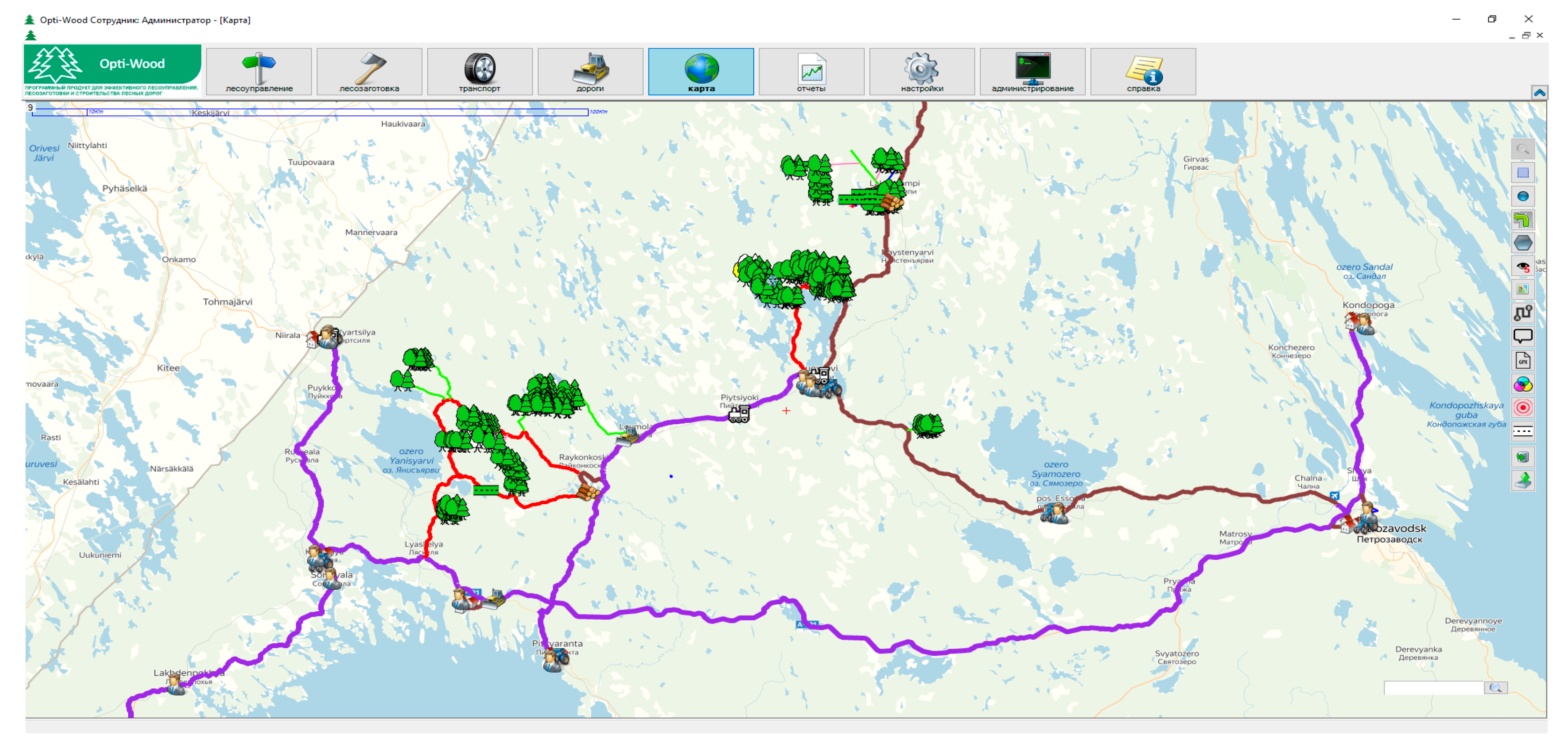
2.4. Implementation

The solution to the problem of optimal planning of wood harvesting and timber supply using the described method was implemented in Opti-Wood software, developed by the Russian IT company Opti-Soft together with researchers of Petrozavodsk State University [43] (Figure 1).

At the tactical level, Opti-Wood supports the planning of wood harvesting and timber supply, scheduling of wood harvesting and timber transport machines [10,11], planning of forest road construction and maintenance, scheduling of harvesting sites allocation, etc. At the operational level, the software supports the routing of timber trucks.

A core component of Opti-Wood is an optimization model that takes into account all important features of wood harvesting production in Russia and original optimization algorithms.

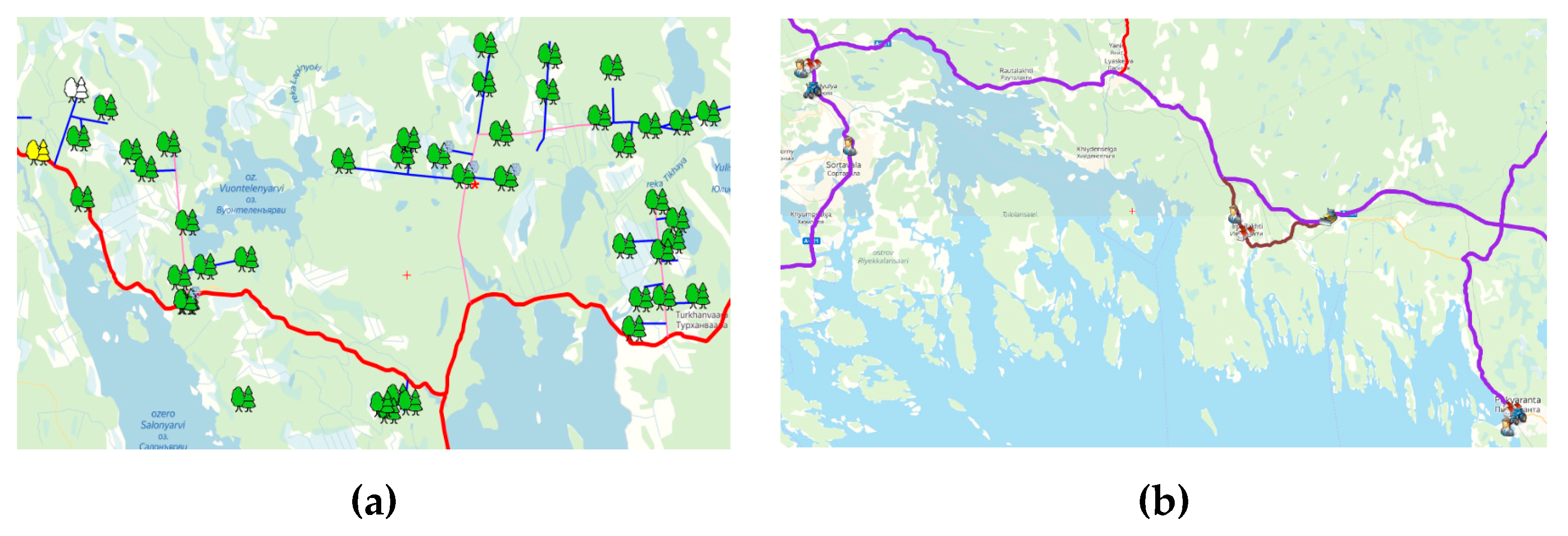
Another main component of Opti-Wood is the road network map with various objects attached to it: harvesting sites, intermediate storage areas, consumer demand points (storage), garages, terminals, quarries, etc. The spatial distribution of accessible harvesting sites (Figure 2a) and other objects (Figure 2b) strongly affects the calculation results. The accessibility of a harvesting site means both transport and organizational accessibility (i.e., the availability of information about the site needed for planning).

3. Results

We tested the methods and algorithms on a case study from a forest company in southern Karelia (Figure 1) with a planning horizon up to a year. This case study involved 198 sites and 14 machines harvesting up to 200,000 cubic meters from an available stock volume of about 300,000 cubic meters. The calculation time on a personal computer (Intel Core i7-4790, 3.6 GHz CPU, 16 Gb RAM) in every case was under 5 min. Results are presented in

Table 1. Plan calculation results.

Plan	Total Volume Harvested (1000 m3)	Total Cost (million rubles)	Total Revenue (million rubles)	Profit (rubles/m3)	Profit (Actual) 1 (rubles/m3)	Increase (%)
1	167.9	237.2	441.5	1217	1153	5.5
2	172	254.6	515.9	1520	1431	6.2
3	145.2	196.4	428.9	1431	1310	9.2
4	128.1	217.7	388.4	1332	1228	8.5
5	186.8	304.2	569.5	1420	1305	8.9

¹ Observed profit at the forest company without using Opti-Wood software.

,

Table 2. Main cost categories (million rubles).

Plan	Total	Harvesting	Transportation	Road Construction
1	237.2	108.2	72.8	56.2
2	254.6	111	85.8	54
3	196.4	92.1	69.3	32.5
4	217.7	82.3	64.3	69
5	304.2	121.2	95.8	83.9

and

Table 3. Machinery utilization.

Plan	Total Volume Harvested (1000 m3)	Hours Worked	Fleet Utilization Rate	Total Time for Machinery Relocation (hours)	Highest Possible Productivity (1000 m3)
1	167.9	19,137	0.88	63.41	190.8
2	172	19,093	0.89	64.44	193.2
3	145.2	16,225	0.96	143.64	151.2
4	128.1	13,656	0.88	77.46	145.4
5	186.8	20,339	0.95	54.55	196.6

.

Therefore, the proposed numerical method and the algorithm implemented based on it raise the profit by 5% to 10% with given harvesting volumes over the annual planning horizon.

According to our modeling experience, the most significant factors for constructing an effective plan are the spatial locations of sites and consumers and the distribution of wood harvested on a site by product type, which depends on initial stand characteristics.

According to this optimal harvesting plan, other modules of Opti-Wood software were used to automatically calculate an optimal harvesting schedule, in which particular machinery is assigned to each harvesting site included in the plan for a precise operating period (Table 3, Figure 3). The objective of this problem was to minimize total machine relocation. A description of the applied heuristic and metaheuristic methods is provided in [10].

4. Discussion

The proposed approach allows the creation of cost-effective harvesting plans, taking into account specific features of wood harvesting in Russia. The practical feasibility of the created plans was confirmed by specialists of several forestry companies in Karelia and other regions of Russia.

As a disadvantage of the approach from the application standpoint, we note that it works with a limited list of harvesting sites and with fairly precise details, but not with the entire leased forest territory. Therefore, the solution is optimal only within the given list of sites. However, this approach is justified in practice, because most Russian companies do not have information about all of their leased forest territory with sufficient detail for adequate decision making. Moreover, this information is not always in digital form. Knowing precise details about harvesting sites is quite critical to ensure good quality of the plan: If incomplete or approximate initial data are supplied, the system would plan sales of nonexistent volumes of products or would not consume all harvested volume. Planning based on more detailed information is the next step toward more precise supply and demand matching. So, this approach stimulates forest companies to verify information about harvesting sites before planning. Forest companies can use all available means of updating information. Whereas state forest inventory is carried out in a certain order, while waiting for their turn, companies often update information by themselves or by involving private contractors that use modern IT to collect and analyze stand data, e.g., data from satellite, airborne, unmanned aerial vehicles, global positioning systems, sensors, devices, analytical and communication tools [2], laser scanning and complex algorithms for processing raw data.

This work is usually performed gradually over several years. In addition, planning for the whole territory will significantly increase the number of objects, and consequently the calculation time.

Among other results, the proposed approach allows the identification of sites where harvesting would not be effective in current conditions. With such sites identified, forest management activities may be considered, e.g., thinning, etc. Automation and support of such planning may become one direction for further development of Opti-Wood software.

The achieved 5% to 10% increase in profit is generally in line with improvement rates reported by several other research teams [4]. It should be noted here that a one-to-one comparison of different approaches is difficult to undertake, since in every case results depend on particular production conditions and the quality of original “manual” planning. The models described in [3,7,8,9] take into account many factors considered in the proposed model, however, these models fall short in accounting for Russian conditions as they omit such important factors as annual allowable cut, harvesting sites adjacency rules, and seasonal accessibility of harvesting sites.

As a computational disadvantage of this approach, we note the need to take into account integer convex hull coefficients ${\lambda }_{\omega }, \omega \in {\mathsf{\Omega }}_u u\in U$ when using the modified branch and bound method. This leads to re-solving the original problem with an additional constraint at each step of the current set partition, which slows the calculation time. A possible remedy is the “warm” start, i.e., using the already found basis plan with a partial solution of the problem for new constraints. The effect of this modification on the solution quality of the main problem is another further research direction.

5. Conclusions

This paper describes the developed approach to optimizing wood harvesting planning and distribution of produced assortments between consumer demand points, taking into account a large number of legislative and technological conditions and limitations specific for Russian forestry companies.

A mathematical model of the problem is formulated and analyzed. This multicriteria Boolean nonlinear programming problem has a large dimension, two linear objective functions, and several nonlinear relationships between parameters.

The original problem was transformed to a block linear programming problem of large dimension. An effective numerical solution method is proposed based on a multiplicative simplex method with column generation within Dantzig–Wolfe decomposition, using heuristics to determine a feasible solution based on the branch and bound method.

The proposed mathematical model and numerical methods for solving the described problem were implemented in the Opti-Wood software tool and tested on real production data from a forest company in southern Karelia. An increase in profit by 5% to 10% was observed, measured as revenue from the sale of products, net of harvesting and transportation costs.

Some disadvantages of the proposed approach are discussed, including the need to have a substantial amount of fairly detailed information about harvesting sites and stand characteristics, which is not always fully available. This lack of information is not specific to Russia, but can also be observed in other countries. Some managerial and technological measures are mentioned regarding how to identify and fill in the missing data.