Article

Monitoring Broadscale Vegetational Diversity and Change across North American Landscapes Using Land Surface Phenology

by
Bjorn-Gustaf J. Brooks
1,2,*,
Danny C. Lee
1,
Lars Y. Pomara
1 and
William W. Hargrove
1
1
Eastern Forest Environmental Threat Assessment Center, USDA Forest Service, 200 W.T. Weaver Blvd., Asheville, NC 28804, USA
2
North Carolina Institute for Climate Studies, North Carolina State University, 155 Patton Ave., Asheville, NC 28801, USA
*
Author to whom correspondence should be addressed.
Forests 2020, 11(6), 606; https://doi.org/10.3390/f11060606
Submission received: 9 April 2020 / Revised: 19 May 2020 / Accepted: 25 May 2020 / Published: 27 May 2020
(This article belongs to the Special Issue Forest Biodiversity Conservation with Remote Sensing Techniques)

Abstract

:
We describe a polar coordinate transformation of vegetation index profiles which permits a broad-scale comparison of location-specific phenological variability influenced by climate, topography, land use, and other factors. We apply statistical data reduction techniques to identify fundamental dimensions of phenological variability and to classify phenological types with intuitive ecological interpretation. Remote sensing-based land surface phenology can reveal ecologically meaningful vegetational diversity and dynamics across broad landscapes. Land surface phenology is inherently complex at regional to continental scales, varying with latitude, elevation, and multiple biophysical factors. Quantifying phenological change across ecological gradients at these scales is a potentially powerful way to monitor ecological development, disturbance, and diversity. Polar coordinate transformation was applied to Moderate Resolution Imaging Spectroradiometer (MODIS) normalized difference vegetation index (NDVI) time series spanning 2000-2018 across North America. In a first step, 46 NDVI values per year were reduced to 11 intuitive annual metrics, such as the midpoint of the growing season and degree of seasonality, measured relative to location-specific annual phenological cycles. Second, factor analysis further reduced these metrics to fundamental phenology dimensions corresponding to annual timing, productivity, and seasonality. The factor analysis explained over 95% of the variability in the metrics and represented a more than ten-fold reduction in data volume from the original time series. In a final step, phenological classes (‘phenoclasses’) based on the statistical clustering of the factor data, were computed to describe the phenological state of each pixel during each year, which facilitated the tracking of year-to-year dynamics. Collectively the phenology metrics, factors, and phenoclasses provide a system for characterizing land surface phenology and for monitoring phenological change that is indicative of ecological gradients, development, disturbance, and other aspects of landscape-scale diversity and dynamics.

1. Introduction

The use of remote sensing to characterize vegetation, map spatial gradients, and monitor temporal change has significantly advanced the field of landscape ecology [1,2,3]. This importantly includes applications using measures of surface reflectance (“greenness”) through time to infer properties of the vegetative land cover. Remotely sensed seasonal variation in vegetation (land surface phenology (LSP)) based on such measures is strongly correlated with annual pulses of leaf-out through senescence [4,5,6]. Given appropriate choices of spatial and temporal resolutions, LSP approaches can be used to systematically track vegetation dynamics including disturbance, recovery, and development [7,8]. Beyond providing phenological information, LSP linkages to a wide variety of ecosystem and landscape properties and processes provide insight into large-scale ecological diversity, distributions, and change [4,9,10,11]. Ground-based approaches exist for observing landscape-level vegetation phenology over local areas, but satellite-based LSP is much broader in scale, often spanning biomes with strongly differing phenologies. These differences are useful for indicating ecological gradients and change, but they also present challenges for systematic and consistent continental-scale assessment and monitoring.
Satellite-based LSP from sources such as the moderate resolution imaging spectroradiometer (MODIS) allows large landscape assessment and change diagnosis [12,13]. These measurements cannot distinguish individual tree-crowns. At medium spatial resolutions (250 m in the case of MODIS), a phenological measurement typically reflects aggregate behaviors of multiple plant assemblages, which can be affected by different environmental factors (e.g., harvested and non-harvested patches), or differential responses within a plant assemblage to a common factor (e.g., species-specific drought responses). If environmental factors are strong enough to affect the aggregate surface reflectance signal, temporal and spatial variation in land surface phenology reflects the underlying dynamics of the ecosystem. Examples include biotic disturbances, such as defoliation from insect outbreaks and mortality [14,15,16], and abiotic disturbances tied to regional climate changes [17].
Due in part to complications from scale representativeness and asynchrony, much of the work in LSP has addressed thematically coarse land cover mapping and disturbance monitoring rather than variability along nuanced ecological gradients such as those associated with within-ecosystem plant species compositional and structural change. By contrast, classification schemes which group image pixels into phenologically self-similar clusters allow for quantifying and mapping phenological variation at arbitrarily fine levels of distinction [7,18,19,20]. Successive satellite measurements of a reliable vegetation indicator such as the normalized difference vegetation index (NDVI) are used to build a phenological profile across a year, and annual profiles are clustered. Clustering may be performed on the successive index values themselves or on derived metrics such as growing season start and length [19]. The process of generating metrics and phenological classes (phenoclasses) can be automated for each year to assess change. This approach has been used as a basis for monitoring vegetation dynamics [7].
The capacity to undertake broadscale monitoring of vegetation as it develops and responds to environmental conditions has been expanded by high-performance computing [21,22] and LSP algorithm development [23], but more can be done to boost abilities to interpret phenology across broad scales in a standard way. Further, while clustering approaches elegantly summarize phenological similarity and difference, their interpretation in intuitive phenological terms (e.g., growing season or seasonality) can be challenging when the number of starting variables or metrics is large. An optimal system should be complex enough to provide rich phenological characterization, yet simple enough to allow rapid processing and ready interpretation.
We introduce an LSP method that reduces data volume through a series of annual metric computations to isolate the fundamentally important dimensions of phenological variability. This approach provides intuitive metrics and phenoclass memberships with clear quantitative phenological descriptions for each pixel and year. This quantifies variability over space and time along multiple phenological dimensions amenable to comparison with various ecological, biophysical, and climatological data sets. Phenology data products resulting from our analysis can be explored through our online landscape phenology monitoring system (https://landat.org).
Our process is three-fold and begins by generating phenology metrics (e.g., length of season, average greenness) for each pixel using polar coordinate transformation (PCT). The phenology metrics can be tailored to summarize aspects of biophysical change that are of primary interest. Circular plots of time series data resulting from PCT visualize annual phenology as an explicitly cyclical phenomenon [24,25]. This allows for the efficient calculation of the normal phenological year timing (as distinct from the calendar year), extraction of phenology metrics relative to the phenological year, and enhanced the appearance of anomalous phenology years because departures appear as deviations from the normal annual ellipse.
Next, the metrics are transformed through factor analysis to reduce the data to a set of latent variables (factor scores), reducing the variables needed to represent the annual phenology profile while preserving nearly all of the variability. The factor analysis reveals fundamental dimensions of phenology which are intuitive because they correspond to common interpretations of annual phenology, and because their variability has straightforward ecological relevance. Last, the factor scores of each pixel in each year are clustered to yield discrete phenoclasses. Each phenoclass is defined by its mean factor score values, thereby quantifying similarities and differences among phenoclasses. The phenology metrics, factor scores, and phenoclasses can all be mapped to reveal the geography of the various dimensions of vegetation phenological behavior. Tracking year-to-year changes either in factor scores or phenoclass membership provides a quantitative means of assessing landscape dynamics.
An important advantage of polar coordinate transformation is that it facilitates the comparison of locations across large domains. Through PCT, each pixel is standardized to its own phenology calendar, regardless of when its phenological minimum occurs during the year. As a result PCT standardizes each pixel for its own latitudinal, elevational, or climatic characteristics. PCT provides a new capacity to measure phenology relative to the calendar year or the phenology year of each pixel beginning at its own minimum [25]. This has substantial advantages for phenological analysis at continental scales, especially with respect to climate change. This work focuses on developing a system for monitoring landscapes as they respond to ecological and climatic change.

2. Materials and Methods

2.1. Study Area and Data

The study area data are derived from normalized difference vegetation index time-series data set from the MODIS platform. This is a gap-filled and smoothed product with a 250-m nominal resolution, between 20° and 50° latitude [26]. The full data set consists of 188.6 million pixels spanning the Conterminous US and significant parts of Canada and Mexico, with 46 regularly spaced values per year (an 8-day interval) from 2000 through 2018. Processing procedures for this data set differ from the MYD13Q1 and MOD13Q1 16-day MODIS NDVI products. First, NDVI measurements from Aqua and Terra satellites taken on the same day were merged to enhance representation according to the methodology of [26]. Second, artifacts—primarily clouds—were filtered using maximum value compositing, as described by [27,28]. Last, additional temporal processing was performed to correct for other artifacts including snow cover [29].
While MODIS MCD12Q2 provides metrics that identify phenophase transitions, we use PCT to calculate phenological metrics directly from NDVI time series. An important goal of this approach was to rely on as few assumptions as possible, particularly about trends and trajectories of the phenology cycle. This precluded standard LSP products that identify phenophase transitions by first fitting models to the data and then looking for departures. In addition, our approach allows for the period of least phenological activity to be excluded from the analysis based on user-defined thresholds for the growing season. This aids a comparison across latitudes, as high latitudes tend to have snow cover artifacts during the winter that artificially reduce NDVI. PCT also provides an elegant solution for representing temporal patterns that span across the beginning or end of calendar years, as explained below.

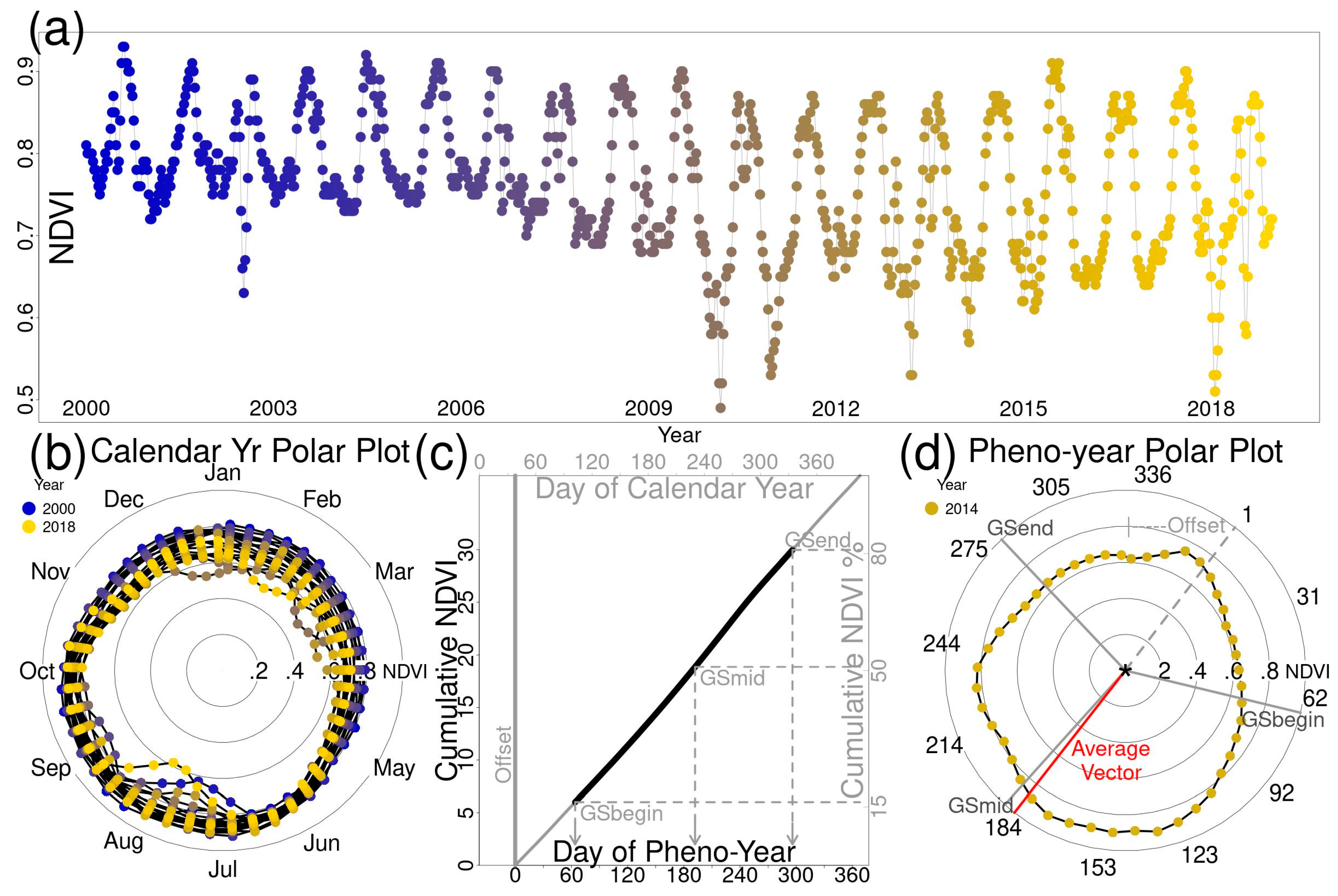
2.2. Polar Coordinate Transformation and Phenology Metrics

Polar coordinates are used in atmospheric sciences, engineering, astronomy, and elsewhere to describe two-dimensional measurements relative to a central reference point (e.g., wind speed and direction). Less commonly, polar transformations have been applied to time series data, treating regular cycles as passes around the polar circle. Surprisingly, PCT has rarely been applied to temporal environmental data (but see [24,25,30,31]).
We applied PCT to land surface phenology as the first step in data analysis. We then calculated a set of milestones and descriptive statistics using transformed data to collectively characterize the phenological year and seasonal differences in terms that were relevant to our interest in landscape analysis (Table 1). The procedure used for PCT is fundamentally the same as commonly found in atmospheric science, e.g., to determine vector averaged wind speed and direction, except here, time is converted into radial coordinates. In the first step the day of the year, d = 1 365 , was converted to radians r using:
r = ( d 365 ) × 2 π
Using r and measured NDVI, v , the time series can be graphed using polar coordinate pairs [ r , v ] . Irregularities in the overlapping orbits around the polar plot reflect variations in the eight-day measurements from year to year (Figure 1b,c).
Summarizing polar coordinate data requires projection onto two-dimensional Cartesian coordinates. Each [ r , v ]   pair was projected on a coordinate plane by applying cosine and sine functions to [ r , v ] as:
x ( r , v ) = v × cos ( r )
y ( r , v ) = v × sin ( r )
Several polar measures were calculated using the mean of x and y , termed x ¯ and y ¯ . These were calculated over n samples within the period of interest, simply as:
x ¯ = i = 1 n x i / n
y ¯ = i = 1 n y i / n
Thus, [   x ¯ , y ¯   ] describes the coordinates of the average vector, which can be projected back into polar coordinates of angular displacement and distance, [   r ¯ , v ¯   ] , using the relationships,
r ¯ = { a t a n 2 ( y ¯ , x ¯ )                                       a t a n 2 ( y ¯ , x ¯ ) > 0     a t a n 2 ( y ¯ , x ¯ ) + 2 π               o t h e r w i s e                            
v ¯ = x ¯ 2 + y ¯ 2
[   r ¯ , v ¯   ] is the resultant vector with a magnitude proportional to the normal (multi-annual) strength of seasonality, and direction indicating the central tendency of NDVI in the annual cycle. Phenological timing varies significantly across large landscapes due to latitudinal, elevational, hydrological and other environmental gradients affecting vegetation. For example, the phenology of deciduous locations across much of the southwest is six months out of phase with much of the Conterminous United States (Figure 2a). Polar coordinate transformation facilitates the calculation of standard metrics, normalized to the customized phenological year of any given pixel, which can clarify similarities in modes of phenological variability while preserving timing differences.
Following the polar transformations shown above, the next step identifies the unique starting date for the phenological year associated with each pixel. This corresponds to the period of least photosynthetic activity, when NDVI values are generally lowest (i.e., winter for most pixels), which rarely coincides exactly with the beginning of the calendar year. The period of least activity is simply the diametric opposite of the average vector [   r ¯ , v ¯   ] , i.e., rotated exactly one-half year ( π radians) from r ¯ . This new angle θ is a complement of r ¯ based on Equation (6) using the full multi-annual time series of NDVI values ( n = 19 × 46 = 874 ) . That is,
θ = { ( r ¯ + π )                     ( r ¯ < π )   ( r ¯ π )             o t h e r w i s e  
We recorded this parameter as the offset (in radians or back-transformed to days) between the beginning of the phenological year and that of the calendar year. The straight line formed by θ and r ¯ bisects the polar graph into two sections of equal area under the multi-annual NDVI profile; the sum of NDVI values clockwise from θ to r ¯ is equivalent to the sum clockwise from r ¯ to θ .
Subsequent phenological metrics (Table 1) were calculated and are reported by their calendar date. The time series of coordinate pairs [ r , v ] was first divided into phenological years, beginning with the first NDVI reading after θ . The initial and final segments of values that occur before θ in the first year and after θ in the final year were omitted, thus resulting in 19     1 phenological years with 46 dates each ( r _ 1 , 1 , , r _ 18 , 46 ) . Within each phenological year, NDVI values were converted to cumulative proportions of the year’s total NDVI accumulation, from zero to one. Proportional values were used to determine benchmarks that defined beginning, middle, and ending growing season dates. Any NDVI threshold, t with range ( 0 , 1 ) , can be used to mark a phenological milestone, J ( t ) , corresponding to the earliest date J when the cumulative proportion exceeds the threshold value t . We chose the phenological milestones J ( 0.15 ) , J ( 0.5 ) , and J ( 0.8 ) to define the beginning (GSbegin), middle (GSmid), and end (GSend) of the growing season (Table 1). These correspond to 15%, 50%, and 80% completion thresholds of the phenological year; other threshold values can be chosen to suit a particular analysis. The length of the growing season (LOS) was simply the number of days (or radians) between J ( 0.15 ) and J ( 0.8 ) (Figure 1c).
Annual measures of NDVI’s central tendency include the mean (mean_NDVI_grw) and standard deviation (std_NDVI_grw) of observed NDVI within the growing season, indicating the average productivity and within-season variability, respectively. We also calculated an average vector for the growing season, AVgrw, ( r ¯ g r w ,   v ¯ g r w ) using Equations (4)–(7) with appropriate n, whose vector length is also a measure of the degree of seasonality. For additional information about the seasonal pattern, we examined the early (GSbegin to GSmid) and late (GSmid to GSend) portions of the growing season separately. We calculated average vectors for both of these periods, indicated by ( r ¯ e a r l y ,   v ¯ e a r l y ) and ( r ¯ l a t e ,   v ¯ l a t e ) , respectively. This yielded two additional vector directions (GSmid_early and GSmid_late) and two additional vector lengths (AVearly and AVlate). Collectively, these vectors and the differences among them provide insights about modality and symmetry throughout the growing season (Figure 1d). All phenological metrics are sensitive to different aspects of growing season variability, as discussed below. PCT analyses were performed in R [32]. Our repository of R code is accessible on GitHub at https://github.com/LandscapeDynamics/PolarMetrics; additional details of the PCT process are in [25].

2.3. Dimensional Reduction and Phenological Classification

Through the process described above, we produced 11 metrics to describe LSP (Table 1). These included six measures describing aspects of seasonality and greenness/productivity, and five timing milestones, i.e., growing season benchmarks recorded as a day of year ( r , in radians). For further analysis as quantitative metrics, these circular timing milestones were transformed using the s i n ( r ) and c o s ( r ) functions such that dates near the beginning/end of the year had similar values. For example, 1 January and 31 December are distant when expressed in radians or days-of-year, but appropriately near in the circular sine-cosine coordinate space. This resulted in five timing variable pairs, e.g., [ s i n ( G S b e g i n ) ,   c o s ( G S b e g i n ) ] . Therefore, the data set that we subjected to factor analysis consisted of 16 variables for each pixel-year combination.
We used factor analysis to reduce the 16 variables to a smaller set of linear combinations (factors) that explained the bulk of the variation across the data, and to help identify core dimensions of phenological variability. We performed a factor analysis using the factanal base stats function in R [32]. Pearson correlation coefficients among the 16 variables were used to calculate factor loadings. The factors having eigenvalues greater than one were retained and rotated using varimax rotation to improve interpretability. The rotated factor pattern (loadings) was then used to generate factor scores for each pixel-year combination.
Factors are continuous variables, and the combination of factor scores assigned to a particular pixel is potentially unique. However, the ecological significance of phenological differences measured by differences in one or more factor-scores is not known a priori. Pixels can be grouped by similarity to facilitate comparisons but implicit in such grouping is the presumption that inter-group differences are more meaningful than intra-group differences. Cluster analysis provided a statistically rigorous means of grouping pixel-years based on their factor scores, identified herein as phenological classes or phenoclasses. The term phenoregion is also used [18], but phenoclass is preferred when pixels can change group membership over time in response to environmental change and when pixels in each group may be widely disjunct geographically. Phenoclasses can be thought of as categorical types into which the multidimensional phenological space has been partitioned, and within which vegetation exhibits a common and characteristic phenological pattern.
We used non-hierarchical k-means clustering [33] where input variables were the factors at the pixel-year level. Objective clustering was used to minimize the error between each of the k representative centroids and the cluster members (pixel-years) using the sum of squares criterion while maximizing the differences between centroids [34]. A k-means clustering approach was used because it is unsupervised and provides several options for seed selection [35,36,37,38,39].
Ensuring that the clustering process begins with high-quality initial seeds typically results in better-separated and more representative final clusters. For our purposes, the seed finding algorithm used in SAS’s “PROC FASTCLUS” [40] was suitable. Several of the more widely used seed finding algorithms [35,36,37,38] were tested and found to produce seeds whose distributions broadly mirrored those of the factor score values. That is, these methods placed the most seeds where most of the factor score values were located, with few seeds outside of that central domain. This, in turn, resulted in final cluster centroids with a similar relation to the original data distribution. Although desirable in many contexts, one consequence when measuring phenological change is that phenoclasses outside of the denser part of the data distribution exhibit both larger intra-cluster and inter-cluster differences, with more widely spaced centroids. For this reason, transitions (changes between phenoclasses) in the sparse data region would only be observed when phenological changes were unusually large, whereas in the denser part of the data distribution only comparatively small changes would be required to elicit phenoclass transitions. The result in ecological terms is that a typical landscape undergoing minor transitions between closely spaced phenoclasses can appear just as dynamic as a strongly disturbed landscape undergoing transitions between widely spaced, uncommon phenoclasses. Thus, a clustering process that tends to result in more uniformly distributed final cluster centroids, as employed here, has advantages in the context of monitoring phenological change.
The number of classes, k , is negatively correlated with how large a step in the factor score space a phenoclass transition represents. Typically, k is chosen a priori based on knowledge of or subjective preference for a given level of division, or it is iteratively determined based on a trade-off between within-cluster and between-cluster deviance. Deviance between groups (i.e., the between sum-of-squares, B S S ) should be large relative to deviance within groups (i.e., the within sum-of-squares, W S S ). This can be measured as B S S /   ( B S S + W S S ) or B S S   /   T S S or (total sum of squares), which approaches 1 as k approaches the number of pixel-years. In the end we chose a 500-class analysis for demonstrative purposes based on (1) optimizing computation, and (2) ensuring that there was sufficient resolution to show relevant ecological divisions, without showing phenology changes due to minor climatic variation, which detracts from our focus on detecting dynamic change.

3. Results and Discussion

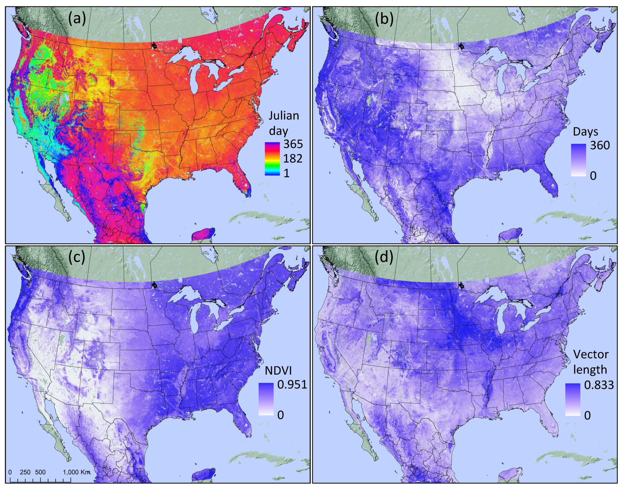
3.1. Phenology Metrics

Each PCT variable measures an intuitive aspect of phenology, e.g., the start of the growing season, the length of the season, and the average growing season greenness. Reducing the many original measurements in each year’s NDVI profile to a suite of PCT variables (Table 1) provides both a substantial reduction in data volume and intuitive ecological characterization. Phenology maps using PCT illustrate differences due to varying environmental drivers, including topography, climate, and land use (Figure 2).
Five of the 11 PCT variables in Table 1 are timing variables, which describe the juxtaposition of the growing season profile with the annual solar cycle. These variables quantify complex patterns in one of the most important components of phenological variability, particularly in the western part of the continent (Figure 2a). For example, the middle of the growing season (GSmid) is coincident with late summer across most of the continent but shows very different timing in the southwestern US, where vegetational phenology is more strongly asynchronous with the solar cycle. There, GSmid varies broadly from September–October in the east (e.g., the Chihuahuan Desert) to February–March in the west (e.g., the Mohave Desert). Along this broadly east–west timing gradient, there is an irregular band through southern Nevada, Arizona, and northwestern Mexico with growing season midpoints between December and January (near Julian days 365 and 1). This regional gradient illustrates the utility of transforming day-of-year phenology metrics to sine-cosine pairs whose values grade appropriately across the end-of-year transition. Moreover, the structure of spatial and temporal gradients in phenology timing is preserved in statistical products such as the factor scores, which take the sine-cosine variables as inputs.
Other PCT variables indicate strong contrast in seasonality and growing season length between much of the northern US (midwestern US through northeastern US and Mississippi River Valley) and the rest of the continent (Figure 2b,d). Landscapes across this broad northern belt are dominated by agricultural crops, prairies, and deciduous trees. The growing season length variable (LOS, Figure 2b) exhibits low values in this region, likely driven by the timing of agricultural activities as well as natural deciduousness. In comparison, more evergreen landscapes in the Pacific Northwest, Eastern Canada, and the southern and southwestern US show larger LOS values. Low seasonality in the latter regions is also indicated by seasonal magnitude (the average growing season vector length, AV_grw, Figure 2d). Although considerable landscape variability is present within regions, the agricultural landscapes of the midwestern US appear to be among the most seasonal systems on the continent, followed by regions dominated by deciduous vegetation such as the central Appalachians and the northeastern US.
Variables quantifying NDVI greenness were correlated with growing season productivity. For example, high growing season NDVI greenness (mean_NDVI_grw) values for the dense forests of the eastern US and Pacific Northwest contrasted with much of the western US (Figure 2c). NDVI greenness also aided in further discriminating regional and landscape phenologies. Consider, for example, that on the basis of length of season (LOS) alone, the Pacific Northwest and Mountain West were difficult to distinguish (Figure 2b). However, through mean_NDVI_grw (Figure 2c), the ecological distinction was clear. The high NDVI of productive, evergreen vegetation in the Pacific Northwest contrasted sharply with lower values in the intermountain and mountain west regions where sparser, more dry-adapted evergreen vegetation dominates.

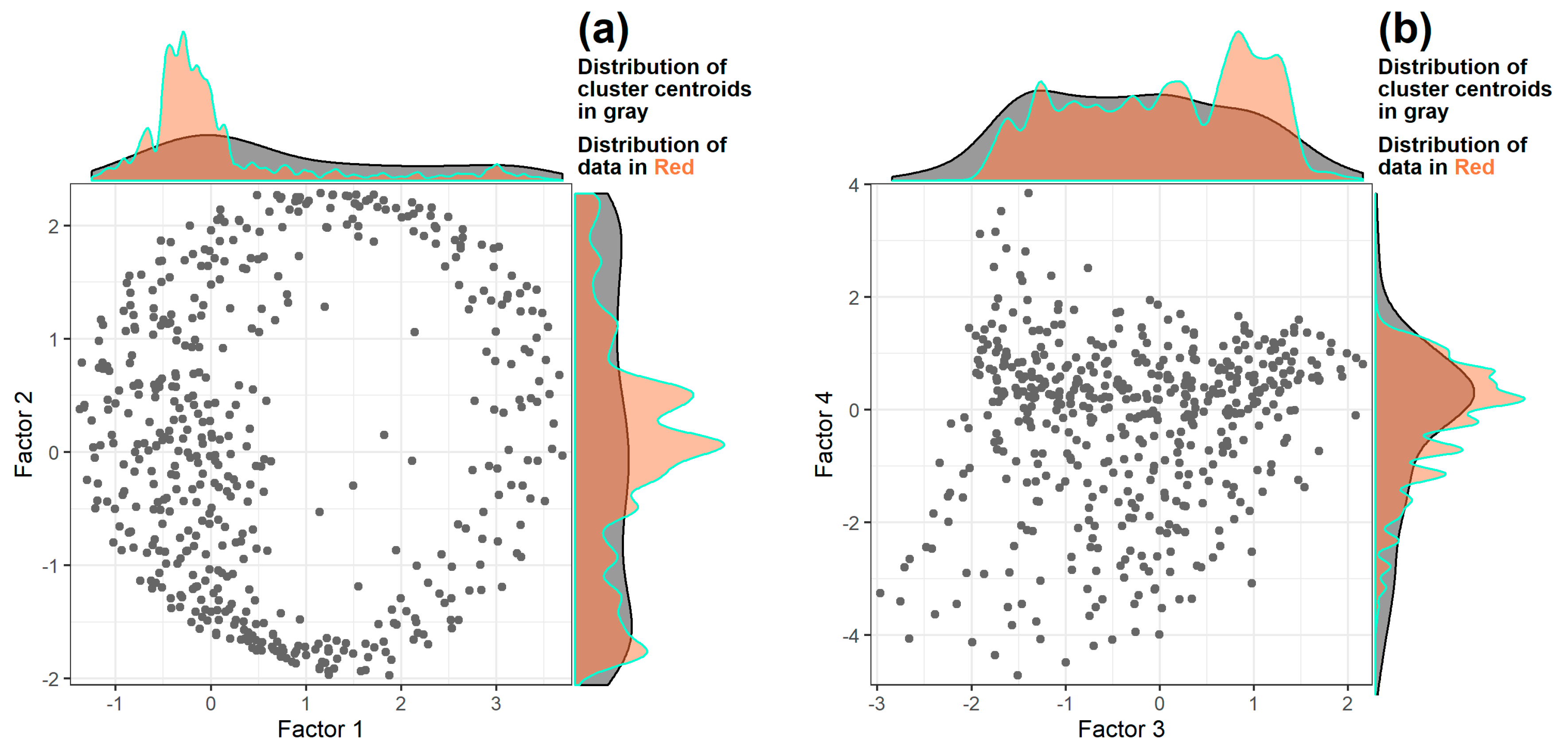
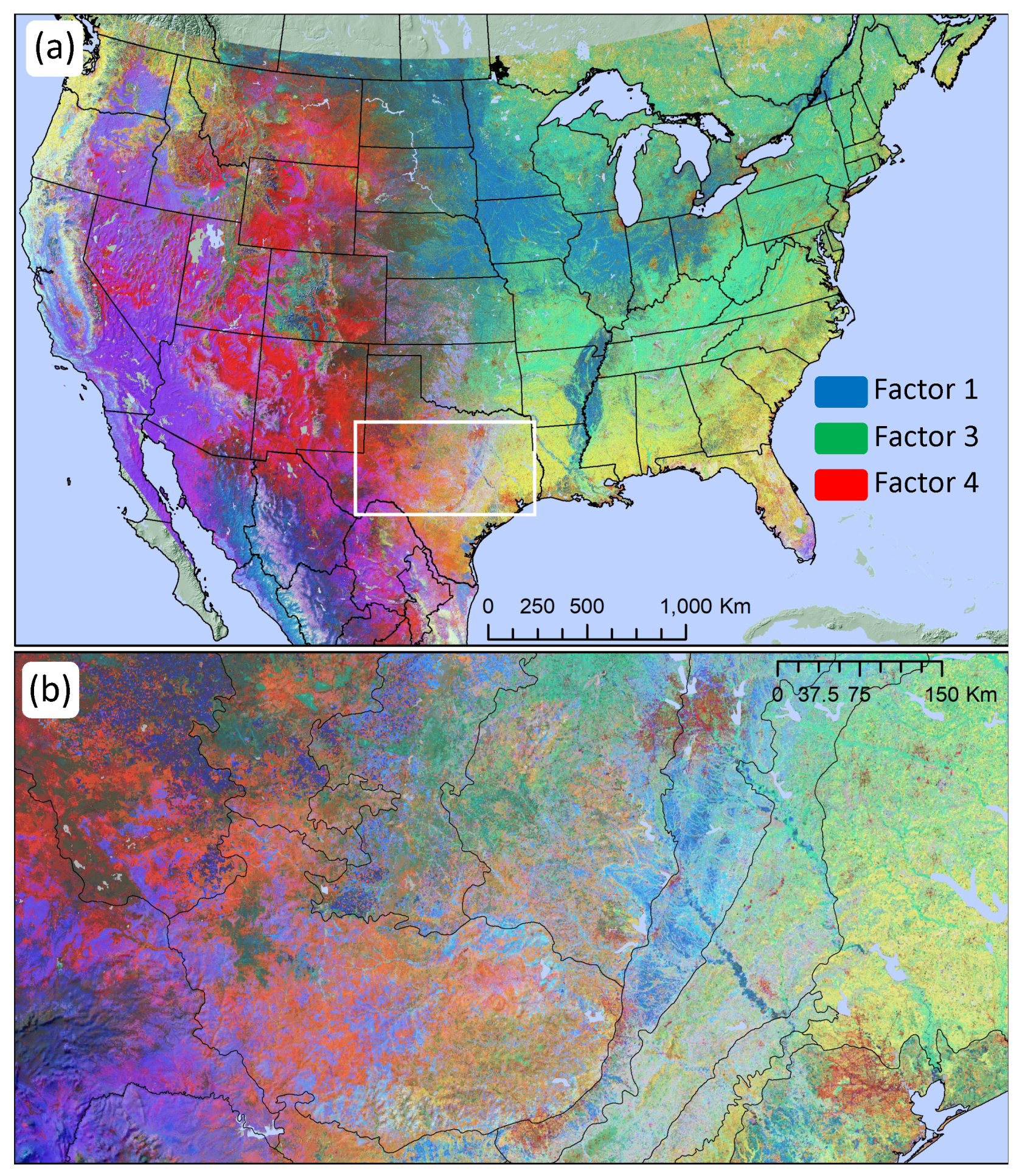
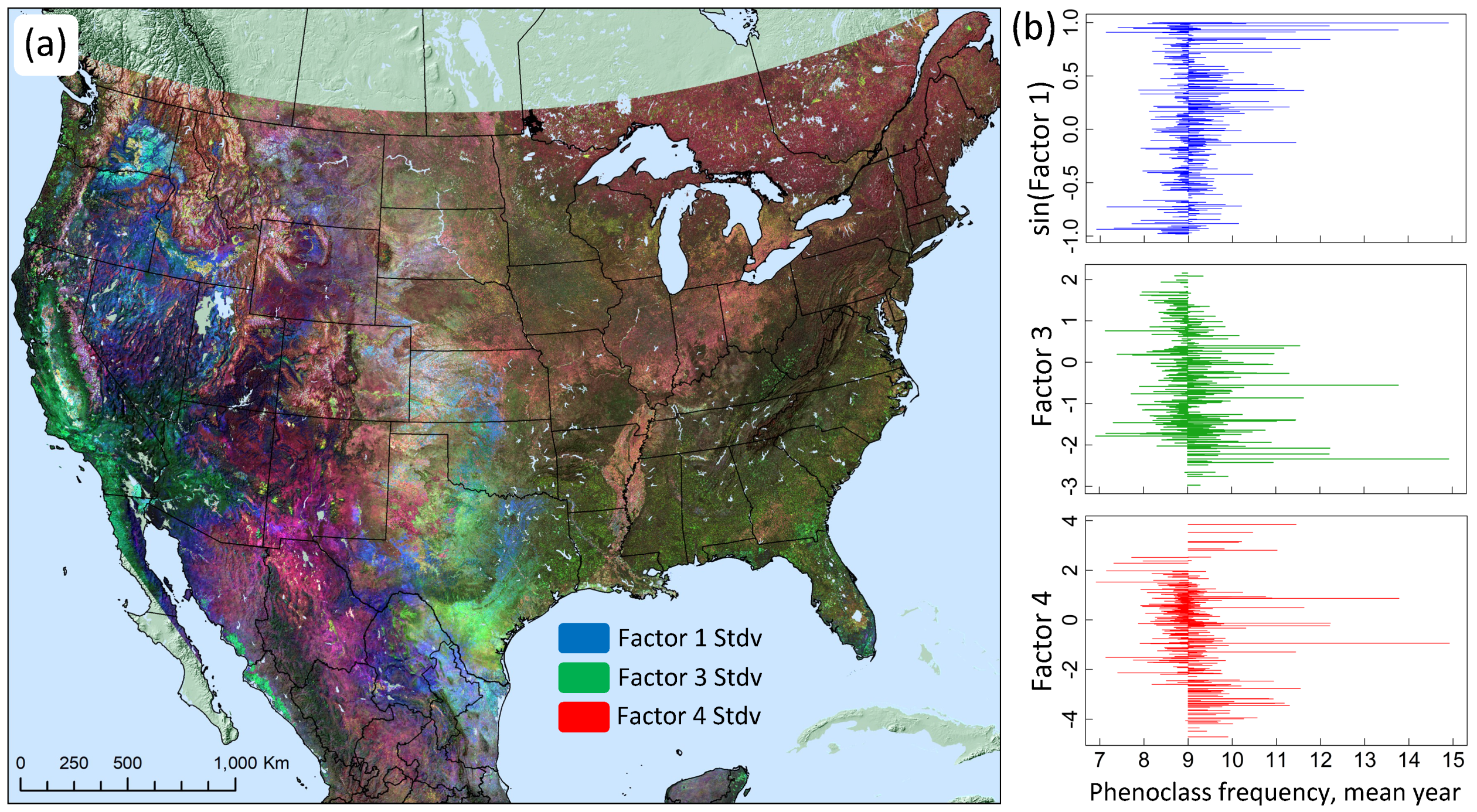
3.2. Dimensional Reduction

Factor scores provide a small, orthogonal set of variables that describe phenological pattern, and are a concise means of quantifying spatial (among-pixels) and interannual (within-pixel) differences in phenology. While PCT reduced the data volume by two thirds (46 variables per year to 16), a further reduction in data volume and increased explanatory power per variable was achieved through factor analysis. There were four factors with eigenvalues greater than 1, which collectively explained over 95 percent of the variance among the 16 variables in the PCT data set (Table 2).
Rotated factor loadings discriminate three main phenology characteristics: timing, productivity, and seasonality. Rotated factors 1 and 2 are heavily loaded on the timing variables (GSbegin_cos, GSbegin_sin, etc.), and together explain 58 percent of the variance in the data. This indicates that most of the observed differences in phenology are simply determined by when milestones occur. The complementary loadings of factors 1 and 2 (Table 2) indicate that two dimensions are required to represent circular annual timing as expressed through the sine and cosine variables (Figure 3). Factor 3 explains an additional 23% of the variance and was heavily loaded on variables associated with vegetative productivity as reflected in higher NDVI values, (i.e., mean_NDVI_grw) and the vector length variables (AVgrw, AVearly, AVlate). This is not surprising, as NDVI is one of two measures used to calculate the vector lengths. Factor 4 had heavy loadings for length of season (LOS) and variability in NDVI (std_NDVI_grw) and is referred to here as “seasonality.” Note that due to the signs of the loadings, factor 4 values related inversely to seasonality. Thus, high LOS values and low variation in NDVI result in high factor 4 values, whereas short growing seasons with high intra-season variability result in low factor 4 values. Our interpretation of factor 3 and 4 loadings is that while several of the original variables reflect mixtures of seasonality and productivity, these components are separable and result in two orthogonal factors.
The false-color composite continental map of phenological variability shown in Figure 4 was generated for an individual phenological year by assigning one of the timing factors (factor 1) in combination with the productivity and seasonality factors to blue, green, and red, respectively. This visualization illustrates that the combined factors provide a nuanced description of phenological variation, and collectively are a robust indicator of gradients in ecological and biophysical diversity at landscape, regional, and continental scales. For example, agriculture-dominated landscapes across the US Midwest corn belt and the Mississippi River Valley, where the timing of planting and harvest are synchronized and highly regular at regional scales, show internal similarity that distinguishes them from other regions.
The factor scores also quantify phenological change within pixels. We used a false-color composite mapping approach to illustrate magnitudes of inter-annual variability in the same three factors (Figure 5). For example, grassland and shrubland regions from the Dakotas to south Texas show high inter-annual variability across all factors, whereas forest and desert regions are more stable. Most regions show distinctive mixtures of variability in some phenological characteristics and stability in others.

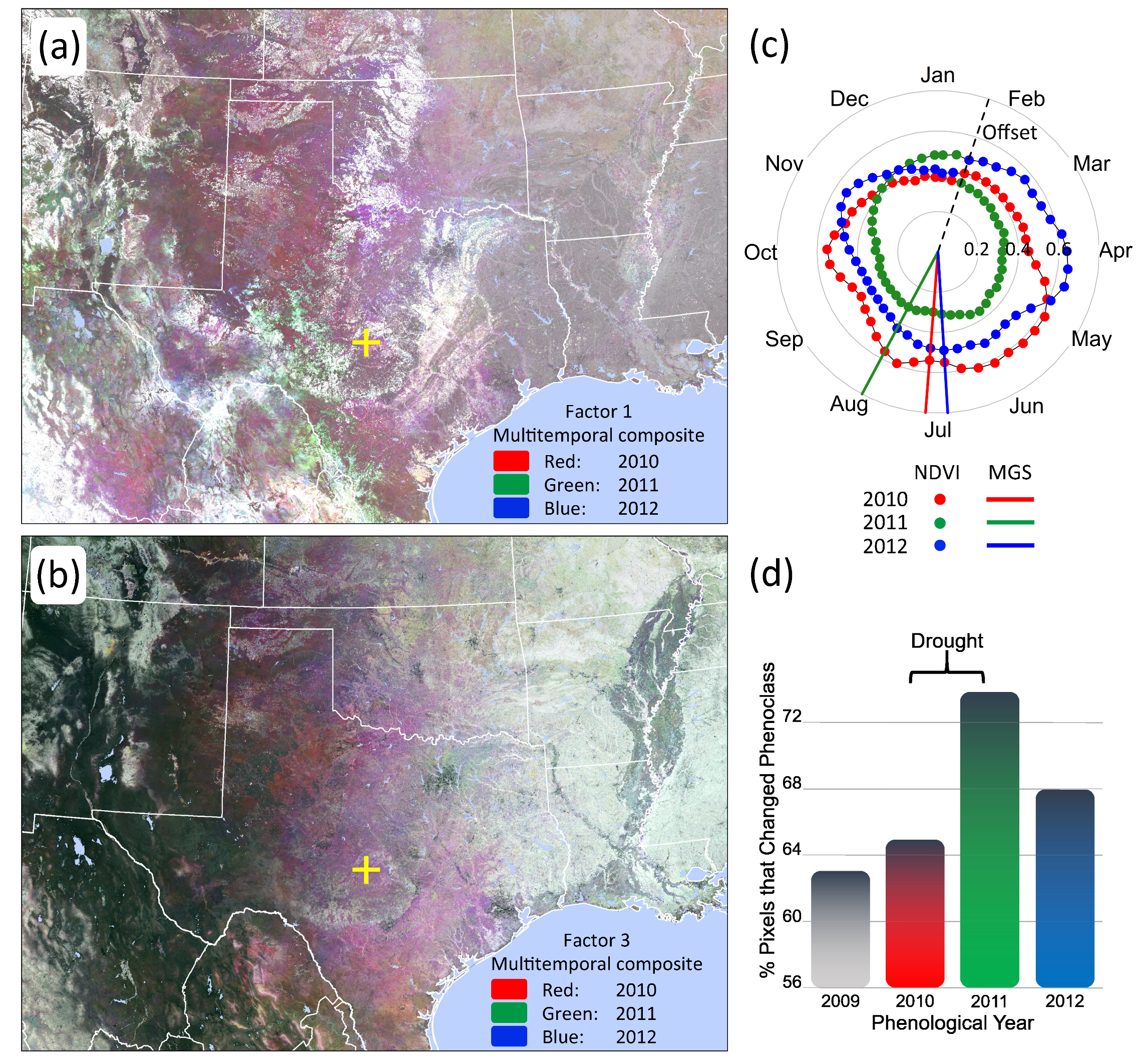
3.3. Phenological Classification

Transitional changes of a pixel from one phenoclass to another between years is determined by the relative position of cluster centroids in the four-dimensional factor score space. Each centroid represents the “center of mass” of a cluster group (i.e., phenoclass) in that space. The phenoclass centroids exhibit different distributions along each of the four factor dimensions, and in three of those dimensions the values are concentrated about a central tendency (Figure 3). As discussed above in Section 2.3, we used a clustering approach with a seed finding algorithm that produced more uniformly spaced centroids, so that the centroid distributions are more uniform than the underlying factor score data. This was done to reduce bias in phenoclass change detection that would otherwise occur when counting transitions for phenoclasses that occurred near the central distribution of the data. This difference is especially evident in the factor 1 and 2 dimensions, wherein the circular joint distribution of timing factors is well-represented by fairly evenly distributed phenoclasses (Figure 3a). Utilizing a more uniform cluster centroid distribution allows for a more ecologically consistent measure of change from one phenoclass to another. Ultimately, classifying continuous factor scores into discrete phenoclasses provides a basis for measuring transitional jumps between phenological states, which can help in identifying meaningful ecological change.
Note that a phenoclass map will illustrate spatial and temporal patterns effectively identical to those evident in Figure 4 and Figure 5, which explicitly map three factor scores as red-green-blue (RGB) composites. This is because phenoclasses preserve factor score values in discretized form, with each phenoclass defined by its centroid’s four factor values. The greater the number of phenoclasses produced by a given analysis, the more closely a phenoclass map will approximate continuous, rather than discrete, factor score variability.
Our results demonstrate that temporal variation in phenology is geographically variable (Figure 5a). Moreover, phenoclass change through time can be used to quantify directional phenological change as reflected in the centroid values. For example, changes in the frequency of different phenoclasses at the continental scale suggest directional shifts in timing, productivity, and seasonality over the period of observation (Figure 5b). We can precisely quantify such changes, but we cannot say with certainty that the observed changes are ecologically important. It is possible to examine areas believed to have experienced substantive change, however, and to objectively assess whether land surface phenology provides a useful method for detection.
To illustrate, we examined factor scores and phenoclasses for an area of the south-central US, centered on Texas, known to have been affected by severe drought during October 2010 through September 2011 (Figure 6). Impacts of the drought on vegetation are captured by the phenological response across the immediate drought interval, in terms of both regional factor score variation and frequency of phenoclass changes. A strong difference between the 2011 growing season and the growing seasons of adjoining years 2010 and 2012 is obvious in the multitemporal factor score maps (Figure 6a,b). The extent and severity of short-term drought impacts, including reduced productivity and delayed growing season timing, are evident throughout eastern and central Texas and north across the High Plains. Anomalous factor values in 2011 also drove a more than 8% increase in pixel-level phenoclass transitions (Figure 6d).
Phenoclass transitions provide a wide variety of additional information about landscape condition and change not explored here. Information pertaining to dynamic landscape mosaics, directional ecological change, predictability, and stability over short and long terms can be gathered, for example, by examining multi-pixel landscapes in terms of their factor score and phenoclass composition and dynamics. Because pixels can change phenoclass assignment between years, it is possible to monitor phenological change in a framework of states and transitions. Preliminary analyses using this approach to address phenological evolution, disturbance, recovery, and land management applications look promising.
Note that phenoclasses are not explicitly land cover classes, although there may be congruence between many land-cover types and their signature phenology. Some land-cover types likely exhibit a mixture of phenological responses due to interannual meteorological differences or other factors. Alternatively, some different vegetation classes likely share phenological signatures, e.g., variation in species composition among pine-dominated ecosystems. Examining such relationships could readily be performed using the data products described here.

4. Conclusions

The three-step process of polar coordinate transformation, dimensional reduction using factor analysis, and statistical clustering into phenoclasses proved to be an effective and efficient means of using land surface phenology to characterize and monitor landscape dynamics. PCT allowed a ten-fold reduction in data volume while showing no loss in sensitivity to NDVI change. Multiple PCT-generated phenology metrics provide a rich characterization of the LSP cycle across large areas at high spatial and temporal resolution. Any of these can be used in focused analyses, based on their relevance for particular types of ecological investigations (e.g., climate drift, land degradation, ecological disturbance and recovery).
Developing factor score variables and phenoclasses from PCT variables resulted in a concise, integrative mapping and classification of LSP on an annual basis. Each phenoclass represents the gross phenological timing, productivity, and seasonality of the vegetation within a pixel, and variations in phenology are quantified across years. Movement along the factor dimensions and transitions between phenological states provide quantifiable evidence of ecological change. An advantage for landscape ecologists and others studying phenological variation and change is that landscapes are depicted using intuitive measures (PCT variables) rather than a complex time series of NDVI values.
Vegetation condition and dynamics mediate, in varying degrees, linkages between natural resources of conservation interest in terrestrial systems (e.g., endangered species, ecosystem services, forest products) and their stressors and drivers (e.g., climate change, land use change, wildland fire). Land surface phenology facilitates vegetation monitoring via remote sensing beyond thematically and temporally coarse land use/cover and towards ecologically nuanced gradients and dynamics. As such, the potential applications of large-scale LSP data sets for studying biodiversity and natural resource conservation and management are vast. These include studies of ecosystem resilience and vulnerability, species and resource distribution modeling, conservation planning, and other applications. The data presented here are available for such applications through an actively managed online database and viewer, namely the Landscape Dynamics Assessment Tool (LanDAT, https://landat.org).

Author Contributions

Conceptualization, D.C.L.; Data Curation, B.-G.J.B. and L.Y.P.; Formal Analysis, B.-G.J.B., D.C.L., L.Y.P. and W.W.H.; Investigation, B.-G.J.B. and L.Y.P.; Methodology, D.C.L. and W.W.H.; Project Administration, D.C.L.; Writing-Original Draft, B.-G.J.B.; Writing-Review & Editing, B.-G.J.B., D.C.L., L.Y.P. and W.W.H. All authors have read and agreed to the published version of the manuscript.

Funding

Funding provided by the USDA Forest Service, Eastern Forest Environmental Threat Assessment Center.

Acknowledgments

We thank Forrest Hoffman and Jitendra Kumar (Oak Ridge National Laboratory) whose work with clustering of NDVI time series was influential, and Steve Norman (USDA Forest Service) who helped develop methods for filtering potentially unwanted portions of the year through PCT. This research was supported in part by an appointment to the United States Forest Service (USFS) Research Participation Program administered by the Oak Ridge Institute for Science and Education (ORISE) through an interagency agreement between the U.S. Department of Energy (DOE) and the U.S. Department of Agriculture (USDA). ORISE is managed by ORAU under DOE Contract Number DESC0014664. All opinions expressed in this paper are the authors’ and do not necessarily reflect the policies and views of USDA, DOE, or ORAU/ORISE.

Conflicts of Interest

The authors declare no conflict of interest.

References

  1. White, M.A.; Thornton, P.E.; Running, S.W. A continental phenology model for monitoring vegetation responses to interannual climatic variability. Glob. Biogeochem. Cycles 1997, 11, 217–234. [Google Scholar] [CrossRef]
  2. Zhang, X.; Friedl, M.A.; Schaaf, C.B.; Strahler, A.H.; Hodges, J.C.F.; Gao, F.; Reed, B.C.; Huete, A. Monitoring vegetation phenology using MODIS. Remote Sens. Environ. 2003, 84, 471–475. [Google Scholar] [CrossRef]
  3. Kennedy, R.E.; Yang, Z.; Cohen, W.B. Detecting trends in forest disturbance and recovery using yearly Landsat time series: 1. LandTrendr—Temporal segmentation algorithms. Remote Sens. Environ. 2010, 114, 2897–2910. [Google Scholar] [CrossRef]
  4. Morisette, J.T.; Richardson, A.D.; Knapp, A.K.; Fisher, J.I.; Graham, E.A.; Abatzoglou, J.; Wilson, B.E.; Breshears, D.D.; Henebry, G.M.; Hanes, J.M. Tracking the rhythm of the seasons in the face of global change: Phenological research in the 21st century. Front. Ecol. Environ. 2009, 7, 253–260. [Google Scholar] [CrossRef] [Green Version]
  5. Liang, L.; Schwartz, M.D.; Fei, S. Validating satellite phenology through intensive ground observation and landscape scaling in a mixed seasonal forest. Remote Sens. Environ. 2011, 115, 143–157. [Google Scholar] [CrossRef]
  6. Rodriguez-Galiano, V.F.; Dash, J.; Atkinson, P.M. Intercomparison of satellite sensor land surface phenology and ground phenology in Europe. Geophys. Res. Lett. 2015, 42, 2253–2260. [Google Scholar] [CrossRef] [Green Version]
  7. Hargrove, W.W.; Spruce, J.P.; Gasser, G.E.; Hoffman, F.M. Toward a national early warning system for forest disturbances using remotely sensed canopy phenology. Photogramm. Eng. Remote Sens. 2009, 75, 1150–1156. [Google Scholar]
  8. Kennedy, R.E.; Townsend, P.A.; Gross, J.E.; Cohen, W.B.; Bolstad, P.; Wang, Y.Q.; Adams, P. Remote sensing change detection tools for natural resource managers: Understanding concepts and tradeoffs in the design of landscape monitoring projects. Remote Sens. Environ. 2009, 113, 1382–1396. [Google Scholar] [CrossRef]
  9. Cleland, E.E.; Chuine, I.; Menzel, A.; Mooney, H.A.; Schwartz, M.D. Shifting plant phenology in response to global change. Trends Ecol. Evol. 2007, 22, 357–365. [Google Scholar] [CrossRef]
  10. Polgar, C.A.; Primack, R.B. Leaf-out phenology of temperate woody plants: From trees to ecosystems. New Phytol. 2011, 191, 926–941. [Google Scholar] [CrossRef]
  11. Norman, S.P.; Hargrove, W.W.; Christie, W.M. Spring and autumn phenological variability across environmental gradients of Great Smoky Mountains National Park, USA. Remote Sens. 2017, 9, 407. [Google Scholar] [CrossRef] [Green Version]
  12. Van Leeuwen, J.D.W. Monitoring the Effects of Forest Restoration Treatments on Post-Fire Vegetation Recovery with MODIS Multitemporal Data. Sensors 2008, 8, 2017–2042. [Google Scholar] [CrossRef] [Green Version]
  13. Kleynhans, W.; Olivier, J.C.; Wessels, K.J.; Salmon, B.P.; van den Bergh, F.; Steenkamp, K. Detecting Land Cover Change Using an Extended Kalman Filter on MODIS NDVI Time-Series Data. IEEE Geosci. Remote Sens. Lett. 2011, 8, 507–511. [Google Scholar] [CrossRef] [Green Version]
  14. De Beurs, K.M.; Townsend, P.A. Estimating the effect of gypsy moth defoliation using MODIS. Remote Sens. Environ. 2008, 112, 3983–3990. [Google Scholar] [CrossRef]
  15. Hicke, J.A.; Allen, C.D.; Desai, A.R.; Dietze, M.C.; Hall, R.J.; Hogg, E.H.; Kashian, D.M.; Moore, D.; Raffa, K.F.; Sturrock, R.N.; et al. Effects of biotic disturbances on forest carbon cycling in the United States and Canada, Global Change Biology. Glob. Chang. Biol. 2012, 18, 7–34. [Google Scholar] [CrossRef]
  16. Spruce, J.P.; Hicke, J.A.; Hargrove, W.W.; Grulke, N.E.; Meddens, A.J.H. Use of MODIS NDVI Products to Map Tree Mortality Levels in Forests Affected by Mountain Pine Beetle Outbreaks. Forests 2019, 10, 811. [Google Scholar] [CrossRef] [Green Version]
  17. Van Mantgem, P.J.; Stephenson, N.L.; Byrne, J.C.; Daniels, L.D.; Franklin, J.F.; Fule, P.Z.; Harmon, M.E.; Larson, A.J.; Smith, J.M.; Taylor, A.H.; et al. Widespread Increase of Tree Mortality Rates in the Western United States. Science 2009, 323, 521–524. [Google Scholar] [CrossRef] [Green Version]
  18. White, M.A.; Hoffman, F.M.; Hargrove, W.W.; Nemani, R.R. A global framework for monitoring phenological responses to climate change. Geophys. Res. Lett. 2005, 32, 4. [Google Scholar] [CrossRef] [Green Version]
  19. Gu, Y.; Brown, J.F.; Miura, T.; Van Leeuwen, W.J.D.; Reed, B.C. Phenological Classification of the United States: A Geographic Framework for Extending Multi-Sensor Time-Series Data. Remote Sens. 2010, 2, 526–544. [Google Scholar] [CrossRef] [Green Version]
  20. Zhang, Y.; Hepner, G.F.; Dennison, P.E. Delineation of Phenoregions in Geographically Diverse Regions Using k-means++ Clustering: A Case Study in the Upper Colorado River Basin. Gisci. Remote Sens. 2012, 49, 163–181. [Google Scholar] [CrossRef]
  21. Kumar, J.; Mills, R.T.; Hoffman, F.M.; Hargrove, W.W. Parallel k-Means Clustering for Quantitative Ecoregion Delineation Using Large Data Sets. Procedia Comput. Sci. 2011, 4, 1602–1611. [Google Scholar] [CrossRef] [Green Version]
  22. Mills, R.T.; Kumar, J.; Hoffman, F.M.; Hargrove, W.W.; Spruce, J.P.; Norman, S.P. Identification and Visualization of Dominant Patterns and Anomalies in Remotely Sensed Vegetation Phenology Using a Parallel Tool for Principal Components Analysis. Procedia Comput. Sci. 2013, 18, 2396–2405. [Google Scholar] [CrossRef] [Green Version]
  23. Bolton, D.K.; Gray, J.M.; Melaas, E.K.; Moon, M.; Eklundh, L.; Friedl, M.A. Continental-scale land surface phenology from harmonized Landsat 8 and Sentinel-2 imagery. Remote Sens. Environ. 2020, 240. [Google Scholar] [CrossRef]
  24. Morellato, L.P.C.; Alberti, L.F.; Hudson, I.L. Applications of Circular Statistics in Plant Phenology: A Case Studies Approach. In Phenological Research: Methods for Environmental and Climate Change Analysis; Hudson, I.L., Keatley, M.R., Eds.; Springer: Dordrecht, The Netherlands, 2010; pp. 339–359. [Google Scholar] [CrossRef]
  25. Brooks, B.J.; Lee, D.C.; Pomara, L.Y.; Hargrove, W.W.; Desai, A.R. Quantifying Seasonal Patterns in Disparate Environmental Variables Using the PolarMetrics R Package. In Proceedings of the 2017 IEEE International Conference on Data Mining Workshops (ICDMW), New Orleans, LA, USA, 18–21 November 2017; pp. 296–302. [Google Scholar] [CrossRef]
  26. Spruce, J.P.; Gasser, G.E.; Hargrove, W.W. MODIS NDVI Data, Smoothed and Gap-Filled, for the Conterminous US: 2000–2015; ORNL DAAC: Oak Ridge, TN, USA, 2016. [Google Scholar] [CrossRef]
  27. Prados, D.; Ryan, R.E.; Ross, K.W. Remote Sensing Time Series Product Tool. In Proceedings of the American Geophysical Union, Fall Meeting 2006, San Francisco, CA, USA, 11–15 December 2006. abstract id. IN33B-1341. [Google Scholar]
  28. McKellip, R.D.; Spruce, J.P.; Smoot, J.C.; Gasser, G.E.; Ryan, R.E.; Holekamp, K.; Ross, K. Time Series Product Tool (TSPT) Version 2.0. Available online: https://www.techbriefs.com/component/content/article/ntb/tech-briefs/information-sciences/20965 (accessed on 5 April 2020).
  29. McKellip, R.D.; Ross, K.W.; Spruce, J.P.; Smoot, J.C.; Ryan, R.E.; Gasser, G.E.; Prados, D.L.; Vaughan, R.D. Phenological Parameters Estimation Tool. Available online: https://www.techbriefs.com/component/content/article/ntb/tech-briefs/software/8481 (accessed on 5 April 2020).
  30. Burgan, R.; Hardy, C.; Ohlen, D.; Fosnight, G.; Treder, R. Ground sample data for the Conterminous U.S. Land Cover Characteristics Database; General Technical Report RMRS-GTR-41; U.S. Department of Agriculture, Forest Service, Rocky Mountain Research Station: Ogden, UT, USA, 1999; Volume 13. [Google Scholar] [CrossRef]
  31. Melendez-Pastor, I.; Navarro-Pedreno, J.; Koch, M.; Gomez, I.; Hernandez, E.I. Land-Cover Phenologies and Their Relation to Climatic Variables in an Anthropogenically Impacted Mediterranean Coastal Area. Remote Sens. 2010, 2, 2072–4292. [Google Scholar] [CrossRef]
  32. R Core Team. R: A Language and Environment for Statistical Computing; R Foundation for Statistical Computing: Vienna, Austria, 2020; Available online: https://www.R-project.org (accessed on 26 May 2020).
  33. Sokal, R.R. The Principles and Practice of Numerical Taxonomy. Taxon 1963, 12, 190–199. [Google Scholar] [CrossRef]
  34. Hartigan, J.A. Clustering Algorithms, 99th ed.; John Wiley & Sons, Inc.: New York, NY, USA, 1975; ISBN 047135645X. [Google Scholar]
  35. Forgy, E. Cluster Analysis of Multivariate Data: Efficiency versus Interpretability of Classifications. Biometrics 1965, 21, 768–780. [Google Scholar]
  36. MacQueen, J.B. Some methods for classification and analysis of multivariate observations. In Proceedings of the 5th Berkeley Symposium on Mathematical Statistics and Probability; University of California Press: Berkeley, CA, USA, 1967. [Google Scholar]
  37. Hartigan, J.A.; Wong, M.A. Algorithm AS 136: A K-Means Clustering Algorithm. J. R. Stat. Soc. Ser. C (Appl. Stat.) 1979, 28, 100–108. [Google Scholar] [CrossRef]
  38. Lloyd, S. Least squares quantization in PCM. IEEE Trans. Inf. Theory 1982, 28, 129–137. [Google Scholar] [CrossRef]
  39. Mills, R.T.; Hoffman, F.M.; Kumar, J.; Hargrove, W.W. Cluster Analysis-Based Approaches for Geospatiotemporal Data Mining of Massive Data Sets for Identification of Forest Threats. Procedia Comput. Sci. 2011, 4, 1612–1621. [Google Scholar] [CrossRef] [Green Version]
  40. SAS Institute Inc. SAS/STAT® 14.2 User’s Guide; SAS Institute Inc.: Cary, NC, USA, 2016. [Google Scholar]
Figure 1. Visualizations of NDVI data from one MODIS pixel extracted from Great Smoky Mountains National Park, North Carolina. (a) Time series showing evergreen decline caused by hemlock tree mortality within the pixel. (b) The same data plotted radially in a polar graph. (c) Cumulative NDVI as a function of time. The 15% and 80% milestones define the start and end of the specified growing season within a phenology-centered year. (d) The phenological offset of each cell from the start of the calendar year is used to rotate and standardize the measurement of phenological completion milestones and growing season measures.
Forests 11 00606 g001
Figure 2. Example land surface phenology metric maps for the phenological year 2016 across North America, based on polar coordinate transformed NDVI time-series data. (a) GSmid, the middle of the growing season, illustrates regional variability in the timing of the phenology year. (b) LOS, the length of the growing season. Note short anthropogenic growing seasons of agricultural landscapes across the Corn Belt and Mississippi River valley. (c) Mean_NDVI_grw, the mean growing season greenness, is a proxy for vegetation productivity. (d) AVgrw, the strength of seasonality, distinguishes between evergreen and deciduous vegetation. These variables and others in Table 1 collectively characterize vegetation similarity and difference at regional and landscape scales. For example, dense and productive evergreen vegetation in the Pacific Northwest displays a long growing season centered late in the calendar year, with high mean greenness. Some of these features are shared, while some contrast with other forested systems such as the boreal forest in eastern Canada, Appalachian deciduous forests, and southeastern US mixed conifer/hardwood forests.
Forests 11 00606 g002
Figure 3. Distributions of cluster centroids (k = 500) resulting from cluster analysis, with respect to (a) factors 1 and 2 (timing factors) and (b) factors 3 and 4 (productivity and seasonality factors). The distributions in the margins compare the factor score data to their representative cluster centroids. The more uniform distribution of centroids was chosen intentionally to disperse phenoclass representation across factor-space. The prominent circular distribution of centroids in (a) is a result of the relationship between factors 1 and 2, which are sine and cosine complements of each other. That is, the factor 1 dimension represents a subset of sine, cosine phenology timing variables that mirrors another subset of sine, cosine variables represented by the factor 2 dimension (Table 2). While the fixed relationship of sine and cosine for input dates plots points exclusively on the periphery of a circle, clustered output values can result in internal points as well. The direction of these points indicates seasonal dates, and the magnitude indicates strength of that seasonality. (b) Factor 3 and factor 4 centroid values indicate average NDVI, seasonal amplitude, and variability.
Forests 11 00606 g003
Figure 4. RGB composite based on three of the four factors from Table 2 for the phenological year 2016 (Red, Green, and Blue are associated with phenological Seasonality, Productivity, and Timing respectively). (a) Continental scale. (b) Central Texas is shown with ecoregion boundaries to illustrate local variation. The combined factors provide a nuanced description of phenology and collectively are a robust indicator of gradients in phenological diversity at landscape, regional, and continental scales. Hue and intensity in this image together indicate overall phenological distinctiveness and similarity. For example, the Southeastern US, Atlantic coast, and Pacific Northwest share a relatively low seasonality and high greenness (in the RGB spectrum, yellow results from high R and G values). Likewise, the largely agricultural Corn Belt and Mississippi River Valley are shown to be phenologically similar, as are the forested Appalachian and Great Lakes regions. Color similarity results from both shared low and high values; for example, red in parts of the Colorado Plateau and northern Great Plains results from both low factor 3 (low productivity) values and high factor 4 (weak seasonality). In (b) Land uses are evident, such as urban areas, as are landscape-scale ecological gradients such as between river floodplains and uplands.
Forests 11 00606 g004
Figure 5. Phenological variability over time as indicated by changing factor scores and phenological class frequencies. (a) Standard deviation in factor score values among phenological years, 2000–2017. The RGB color composite indicates variability in three different factors. Lighter tones indicate more active year-to-year dynamics, and dominance of a given color indicates more variability in that factor. (b) Mean year of occurrence of 500 different phenoclasses, weighted by their frequency within years, shows continental trends over time in phenological traits. The x-axis gives the phenological year, where 9 is the center year among years 1 through 17. Line endpoints relative to year 9 give the frequency-weighted mean year of phenoclass occurrence. Y-axes give the phenoclass centroid values for the three factors shown in the map. Factor one is sine-transformed because its factor loadings are on the day-of-year variables. Broadly, phenological variability over time was highest in the center of the continent and at the highest elevations, and included continental trends towards phenoclasses with higher factor 1, lower factor 3, and more extreme factor 4 values.
Forests 11 00606 g005
Figure 6. An historic drought in 2011 in Texas and surrounding states resulted in depressed vegetation productivity, a delayed growing season, and other observable vegetation phenology impacts. RGB multitemporal false color images of (a) factor 1 and (b) factor 3 show both regionally coherent drought impacts and strong local variability (see Table 2: factor 1 is correlated with growing season timing variables, and factor 3 with greenness/productivity variables). Each color band represents a different year. Gray tones indicate similar phenology values for all years 2010–2012 (lighter grays indicate higher values). Purple color in the large central domain indicates that values in 2010 and 2012 were high relative to 2011. In this region, lower factor 1 values correspond to a later growing season. (c) A radial NDVI plot for a single MODIS pixel (yellow cross on maps) reflects reduced greenness and a delayed growing season in 2011 (MGS = Middle of growing season); seasonality impacts are also evident. (d) shows the 2011 drought response as the percentage of pixels in the view frame that changed their phenoclass membership from the preceding year.
Forests 11 00606 g006
Table 1. Description of phenological variables based on polar coordinate transformation (PCT).
TypeVariable NameDescriptive NameUnitsPolar Description
Timing VariablesGSbeginBeginning of growing seasonDaysNumber of days (or radial angle) corresponding to 15% of cumulative annual NDVI
GSmid_earlyMiddle of early growing seasonDaysNumber of days (or radial angle) corresponding to 32.5% of cumulative annual NDVI
GSmidMiddle of entire growing seasonDaysNumber of days (or radial angle) corresponding to 50% of cumulative annual NDVI
GSmid_lateMiddle of late growing seasonDaysNumber of days (or radial angle) corresponding to 65% of cumulative annual NDVI
GSendEnd of growing seasonDaysNumber of days (or radial angle) corresponding to 80% of cumulative annual NDVI
Greenness & Seasonality VariablesLOSLength of growing seasonDaysNumber of days between early and late growing season thresholds
mean_NDVI_grwAverage growing season greennessNDVIAverage NDVI during the growing season (GSbegin to GSend)
std_NDVI_grwVariability in growing season greennessNDVIStandard deviation of NDVI during the growing season
AVearlyMagnitude of early growing season seasonalityNDVILength of the average vector during early growing season (GSbegin to GSmid)
AVgrwMagnitude of entire growing season seasonalityNDVILength of the average vector during entire growing season (GSbegin to GSend)
AVlateMagnitude of late growing season seasonalityNDVILength of the average vector during late growing season (GSmid to GSend)
Theta (Offset) 1Offset between calendar year and start of phenological yearDaysNumber of days between the beginning of the calendar year (1 January) and the start of the phenological year (defined by when the average minimum in NDVI occurs)
1 Offset was not a variable used in analysis but was a timing point used to define the start of the phenological year within which all PCT variables were measured.
Table 2. Factor loadings from factor analysis using varimax rotation. Coefficients smaller than | 0.2 | are not shown. Variable definitions are given in Table 1.
Factor 1Factor 2Factor 3Factor 4
Timing VariablesGSbegin sin−0.8920.3110.244
GSbegin cos0.2830.911
GSmid_early sin 0.959
GSmid_eary cos0.927 −0.2450.202
GSmid sin0.6750.702
GSmid cos0.672−0.662 0.241
GSmid_late sin0.936 −0.2310.215
GSmid_late cos −0.939 0.304
GSend sin0.568−0.689 0.392
GSend cos−0.764−0.579
Greenness & Seasonality VariablesLOS 0.898
mean_NDVI_grw−0.209 0.964
std_NDVI_grw 0.321−0.836
AVearly 0.960
AVgrw−0.247 0.838−0.457
AVlate−0.274 0.859−0.367
Factor 1Factor 2Factor 3Factor 4
Proportional Variance0.2940.2820.2310.145
Cumulative Variance0.2940.5760.8070.953

