Modelling Lichen Abundance for Woodland Caribou in a Fire-Driven Boreal Landscape

Abstract

Woodland caribou (Rangifer tarandus caribou) are reliant on Cladonia spp. ground lichens as a major component of their diet and lichen abundance could be an important indicator of habitat quality, particularly in winter. The boreal forest is typified by large, stand-replacing forest fires that consume ground lichens, which take decades to recover. The large spatial extent of caribou ranges and the mosaic of lichen availability created by fires make it challenging to track the abundance of ground lichens. Researchers have developed various techniques to map lichens across northern boreal and tundra landscapes, but it remains unclear which techniques are best suited for use in the continuous boreal forest, where many of the conflicts amongst caribou and human activities are most acute. In this study, we propose a two-stage regression modelling approach to map the abundance (biomass, kg/ha) of Cladonia spp. ground lichens in the boreal forest. Our study was conducted in Woodland Caribou Provincial Park, a wilderness-class protected area in northwestern Ontario, Canada. We used field sampling to characterize lichen abundance in 109 upland forest stands across the local time-since-fire continuum (2–119 years-since-fire). We then used generalized linear models to relate lichen presence and lichen abundance to forest structure, topographic and remote sensing attributes. Model selection indicated ground lichens were best predicted by ecosite, time-since-fire, and canopy closure. Lichen abundance was very low (<1000 kg/ha) across the time-since-fire continuum in upland forest stands with dense tree cover. Conversely, lichen abundance increased steadily across the time-since-fire continuum in upland forest stands with sparse tree cover, exceeding 3000 kg/ha in mature stands. We interpolated the best lichen presence and lichen abundance models to create spatial layers and combined them to generate a map that provides a reasonable estimation of lichen biomass (R² = 0.39) for our study area. We encourage researchers and managers to use our method as a basic framework to map the abundance of ground lichens across fire-prone, boreal caribou ranges. Mapping lichens will aid in the identification of suitable habitat and can be used in planning to ensure habitat is maintained in adequate supply in areas with multiple land-use objectives. We also encourage the use of lichen abundance maps to investigate questions that improve our understanding of caribou ecology.

1. Introduction

The boreal ecotype of woodland caribou (Rangifer tarandus caribou) have evolved to occupy a niche unexploited by other northern ungulates [1]. Caribou tend to select low-productivity forests where ground lichens are a dominant understory component and have evolved physiological adaptations to consume these lichens as a major component of their diet, particularly in winter [2,3,4]. By frequenting lichen-rich landscapes, caribou can acquire forage and distance themselves from more productive forests which support higher densities of ungulates (e.g., moose (Alces alces)) and thus predators (e.g., wolves (Canis lupus) [1]. However, stand-replacing forest fires are a common occurrence in woodland caribou habitat and because ground lichens are highly flammable, large quantities of lichen are lost in these disturbances [5]. Since lichens are slow-growing, they take several decades to recover following fire [6,7]. Fires therefore create a constantly shifting mosaic of lichen availability across the landscape, which can influence the distribution and habitat selection of woodland caribou [5,8].

Given the importance of ground lichens in caribou ecology, it may be useful to map the abundance of ground lichens across caribou ranges for research and/or management purposes. Ground lichens are typically found in mature conifer stands with sparse canopy closure and nitrogen-poor, acidic substrate conditions [9,10,11]. Proxies for the growing conditions preferred by ground lichens can be found in forest inventory layers, which often contain attributes for stand age, soil type, tree species composition and forest structure (e.g., canopy closure). Most forest inventories utilize ecological classification systems to divide the landscape into discrete vegetation communities called ‘ecosites’. Each ecosite is characterized by consistent physical features (soil type, soil depth, nutrient availability) and the resulting vegetation community (trees, shrubs and herbaceous plants) [12]. Several researchers have used forest inventory layers to predict the occurrence and abundance of ground lichens [13,14,15]. A disadvantage of forest inventory layers is they are generally unavailable for boreal caribou ranges beyond the range of active forest management. In addition, forest inventory layers are typically updated on long time horizons (e.g., 10–20 years) as part of a forest management planning process, which can make it difficult to update lichen abundance maps to reflect changes to ecosite conditions [13].

Remote sensing has become an essential tool in landscape ecology [16], particularly due to the availability of Landsat satellite imagery [17]. Landsat satellites capture images of the Earth’s surface approximately bi-weekly, allowing researchers to update spatial layers as conditions change [17]. Landsat imagery is composed of several spectral bands that capture different portions of the electromagnetic spectrum. The ground lichens caribou eat contain usnic acid, which produces a unique spectral signature in the blue and short-wave infrared wavelengths [18]. Being pale in colour, lichens can also be distinguished from green vegetation using the normalized difference vegetation index [9], which uses the red and near-infrared wavelengths to quantify vegetation greenness (Appendix C) [19]. The unique spectral properties of usnic lichens in the near- and short-wave infrared wavelengths led to the incorporation of the normalized difference moisture index (NDMI; Appendix C) [20] in several lichen remote sensing studies [21,22]. Studies have proven that Landsat spectral properties can be used to obtain reasonable estimates of lichen abundance in northern boreal and tundra systems [18,21,22]. The unique spectral signature of ground lichens can be captured by the moderate spatial resolution of Landsat imagery (30 m pixels) in northern boreal and tundra ecosystems because tree cover is sparse or non-existent [14]. In the continuous boreal forest, which is characterized by relatively dense tree cover, the unique spectral signature of ground lichens may be masked by the tree canopy [14]. Higher resolution satellite imagery such as SPOT 6 (6 m pixels) and QuickBird (2.5 m pixels) may be able to capture the unique spectral signature of ground lichens in densely treed areas [9], but these platforms do not capture the short-wave infrared portion of the electromagnetic spectrum, which has proven useful in modelling lichens in previous studies [18,21].

Landscape nutrition models often integrate remote sensing and Geographic Information System (GIS) data (e.g., topography, disturbances, forest structure) to generate spatial predictions of forage abundance from field observations. Such models have been generated for multiple, wide-ranging mammal species, including grizzly bears [23,24], elk [25] and woodland caribou [26]. Landscape nutrition models can include multiple food types, including seasonally available plant species and prey biomass [24]. Quantifying forage abundance across the landscape can allow researchers to study the influence of nutrition on survival and fecundity [25]. Forage layers can also be used to identify potential high-quality habitats to target for protection or areas of overlap between humans and wildlife that present a high risk of conflict [23]. In conjunction with spatial predictions of predation risk, forage layers can be used to study the tradeoffs between nutrition and predator avoidance experienced by prey species [26,27].

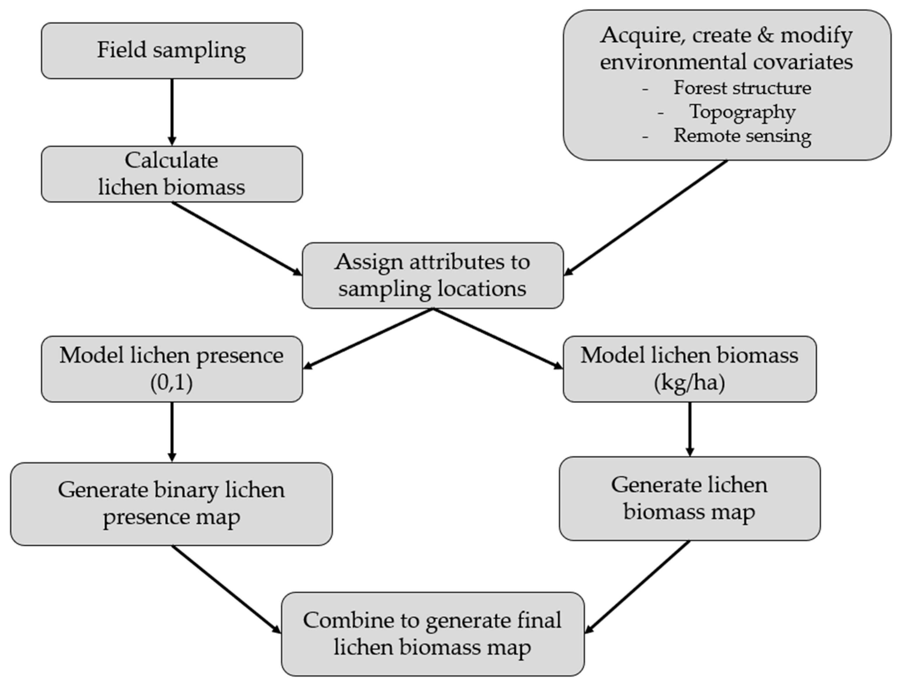
In this study, we create a predictive model of lichen abundance in the boreal forest of Woodland Caribou Provincial Park, in Ontario, Canada and interpolate this model to create a spatial prediction (map) of lichen biomass. We use a regression modelling approach, first conducting field sampling within the study area to parameterize relationships between lichen abundance and environmental conditions (forest type, time-since-fire, canopy closure). We then relate lichen presence and lichen abundance to remote sensing and GIS data and use an a priori model selection procedure to identify the best explanatory variables. We interpolate the top lichen presence and abundance models across the study area and combine them to generate a map predicting lichen biomass (kg/ha). We show that our approach is straightforward and could be applied in other boreal caribou ranges with site-specific field data. Lichen maps could help managers develop more effective conservation strategies for woodland caribou. Managers could use lichen maps to track the availability of this important food resource over time and ensure a constant supply of lichen-rich habitat through resource or fire management planning. Paired with GPS collar locations, lichen maps could be used to identify the quantity of lichen in stands selected by caribou, aiding in the delineation of suitable habitat patches based on available forage resources.

2. Materials and Methods

2.1. Study Area

Our study area encompasses Woodland Caribou Provincial Park, a 5000 km² wilderness-class protected area in northwestern Ontario, Canada (Figure 1) [28]. The park is a part of Pimachiowin Aki, a World Heritage Site that has received international recognition for its intact boreal forest and Indigenous cultural heritage [29]. The region is characteristic of the continuous boreal forest and is characterized by rolling terrain of bedrock outcroppings and numerous small lakes. Elevation varies from 309 m to 430 m above sea level and the park is situated on a plateau slightly elevated above the surrounding area, causing sparse conifer and dense conifer ecosites to compose a large proportion of the study area [30]. Sparse conifer (ecosite B012) occurs primarily on bedrock outcroppings where soils are very shallow (<15 cm) and moisture, nutrient availability, and plant diversity are low [12]. The overstory is dominated by jack pine (Pinus banksiana Lamb.) and the understory plant community consists primarily of Cladonia spp. ground lichens and velvet-leaf blueberry (Vaccinium myrtilloides Michx.). Dense conifer (ecosite B049) dominates upland sites with deeper, rocky soils (>15 cm) and nutrient and moisture conditions are more favourable for plant growth compared to sparse conifer [12]. A mixed overstory of black spruce (Picea mariana (Mill.) BSP) and jack pine characterizes dense conifer ecosites and the understory plant community consists primarily of feathermosses (e.g., Pleurozium schreberi (Brid.) Mitt.) and herbaceous plants (e.g., bunchberry, Cornus canadensis L.)). Small peatlands supporting black spruce and tamarack (Larix laricina (Du Roi) K. Koch) form in bedrock depressions and support an understory plant community dominated by Sphagnum spp. mosses and ericaceous shrubs (e.g., Labrador tea (Ledum groenlandicum Oeder)) [28].

There are no roads or resource development activities, historic or current, within Woodland Caribou Provincial Park. Development is limited to portage trails, campsites and several fly-in fishing camps. Large, frequent forest fires persist as an integral component of the local ecosystem due to a dry, continental climate [28]. The average annual area burned in the park over the last 30 years (1985–2015) is 0.6%, above the average for northern protected areas in Canada [31]. The study area is home to woodland caribou belonging to the Owl-Flinstone and Atikaki-Berens ranges in Manitoba and the Sydney and Berens ranges in Ontario [32].

2.2. Methods Overview

We combined field sampling with spatial environmental covariates to generate a map of lichen biomass for our study area (Figure 2). First, we conducted vegetation surveys to quantify lichen cover and canopy closure in sparse conifer and dense conifer ecosites. We used conversion factors to estimate the stand-level lichen biomass (kg/ha) of each sampling location. Second, we derived nine environmental covariates from remote sensing and GIS data. Third, we assigned our field observations and environmental covariates to the GPS waypoint of each sampling location. We then used generalized linear models to predict lichen presence and lichen biomass as a function of a priori hypotheses built from our environmental covariates. We used model selection to identify the best candidate model and interpolated each top model to generate lichen presence and lichen biomass maps, which we combined to generate a final lichen biomass map for the study area.

2.3. Field Sampling

To quantify lichen abundance, we conducted vegetation surveys at 109 sampling locations within and adjacent to Woodland Caribou Provincial Park from June-August 2018. We selected sampling locations based on time-since fire, stratified into decadal classes (Figure 3; range = 2–119 years post-fire). We confirmed time-since-fire at sampling locations using an increment bore. Due to access constraints and the dominance of upland conifer in the study area, we constrained sampling to dense conifer and sparse conifer ecosites. Within each time-since-fire class we selected an equal number of sampling locations in each ecosite using a forest inventory map.

We accessed sampling locations by canoe and portage within the park and by truck in adjacent areas. At each sampling location, we established a start point 25 m from the edge of the mapped ecosite boundary and used a fiberglass tape to establish a 50 m transect oriented in a primary or secondary compass direction (Figure 4). We placed a 1 m² quadrat at the 5 m, 15 m, 25 m, 35 m and 45 m marks of the transect to conduct five vegetation surveys per sampling location. We recorded the xy coordinates of each sampling location at the 25 m mark of the transect with a handheld GPS unit (accuracy ± 5 m). We spaced sampling locations a minimum of 100 m apart to reduce spatial autocorrelation.

For each 1 m² quadrat, a single observer visually estimated the percent cover of each of the six most common Cladonia spp. ground lichens in the region (

Table 1. Cover-to-biomass (g/cm²) conversion factors for the six most common Cladonia spp. ground lichens found in northwestern Ontario, Canada. Species classification and conversion factors are from McMullin et al. (2011) [33].

Lichen Species	Cover-to-Biomass Conversion Factor (g/cm2)
Cladonia rangiferina (L.) Nyl.	0.10500
Cladonia arbuscula (Wallr.) Flotow	0.08593
Cladonia uncialis (L.) F.H. Wigg.	0.10263
Cladonia gracilis (L.) Willd. ssp. turbinata (Ach.) Ahti	0.14895
Cladonia stellaris (Opiz) Brodo	0.11618
Cladonia stygia (Fr.) Ahti	0.15145

) and used a concave spherical densiometer to estimate the canopy closure above the quadrat. We recorded lichen cover for the sampling location by taking the average of the total lichen cover of each quadrat. Similarly, we recorded a single canopy closure value for each sampling location as the average value from the five quadrats. To derive estimates of lichen biomass, we multiplied the cm² area of the quadrat covered by each lichen species by its corresponding cover-to-biomass conversion factor (developed by McMullin et al. (2011); Table 1) [33]. We validated the conversion factors for use in our study area using destructive sampling (Appendix A). We estimated stand-level lichen biomass (kg/ha) for each sampling location by adding the biomass estimates for each quadrat, converting from g to kg and multiplying by 2000 (see Appendix B for example calculation). We assigned the stand-level estimates of lichen cover, canopy closure and lichen biomass to the GPS waypoint of each sampling location for use in spatial modelling.

2.4. Environmental Covariates

We selected nine environmental covariates (

Table 2. Description of covariates used to model lichen presence and abundance as a function of forest structure, topographic and remote sensing attributes. Additional descriptions of each covariate layer are provided in Appendix C.

Covariate	Source	Data Acquisition	Original Resolution
Ecosite	[39]	2009–2015	polygons at 1:8000
Canopy closure	[39,40,41,42,43]	2009–2018	polygons at 1:8000; polygons of fires ≥ 40 ha; 30 m
Time-since-fire	[40,41]	1929–2013	polygons of fires ≥ 40 ha
Elevation	[44]	2019	30 m
Slope	[44]	2019	30 m
Blue reflectance	[42,43]	2014	30 m
Short-wave infrared (SWIR2) reflectance	[42,43]	2014	30 m
Normalized difference vegetation index (NDVI)	[42,43]	2014	30 m
Normalized difference moisture index (NDMI)	[42,43]	2014	30 m

) supported by the literature to generate spatial models of lichen presence and lichen biomass [9,15,18,21,34,35]. The details of how the covariate layers were created are found in Appendix C. Note that the canopy closure layer was generated using a generalized linear model with forest inventory data, field measurements, time-since-fire and normalized difference vegetation index (NDVI; Appendix C). We converted all polygon datasets to rasters with 30 m pixels in ArcGIS 10.5 [36]. We resampled all covariate layers to have matching 30 m pixels and subsequently assigned values of each of covariate to the GPS waypoint of each sampling location using the mask() and extract() functions in the raster package in R version 3.6.0 [37,38]. This enabled us to subsequently relate lichen presence and biomass to forest structure, topographic and remote sensing attributes.

2.5. Spatial Modelling

We used our environmental covariates to generate a set of seven candidate models (

Table 3. Name and structure of candidate models used to predict lichen presence (0,1) and lichen abundance (biomass, kg/ha) as a function of forest structure, topographic and remote sensing attributes. Covariates within the same model have a Pearson’s correlation coefficient < |0.6|. TSF = time-since-fire, Canopy = canopy closure, NDVI = normalized difference vegetation index, NDMI = normalized difference moisture index, SWIR2 = short-wave infrared reflectance (details in Appendix C).

Model Name	Model Structure
Base	Lichen ~ TSF + Ecosite + Canopy
Elevation	Lichen ~ TSF + Ecosite + Canopy + Elevation
All Topography	Lichen ~ TSF + Ecosite + Canopy + Elevation + Slope
NDVI	Lichen ~ TSF + Ecosite + Canopy + NDVI
NDMI	Lichen ~ TSF + Ecosite + Canopy + NDMI
Blue Reflectance	Lichen ~ TSF + Ecosite + Canopy + Blue
SWIR2 Reflectance	Lichen ~ TSF + Ecosite + Canopy + SWIR2

) based on a priori hypotheses. Our base model includes ecosite, canopy closure and time-since-fire, which we anticipated would be the strongest predictors of lichen abundance. Each additional candidate model built on the base model by adding a topographic or remote sensing covariate. Covariates in the same candidate model have a Pearson’s correlation coefficient < |0.6| to reduce collinearity within candidate models. We included a statistical null model (intercept) to assess the robustness of our candidate models.

To generate a raster with cell values representing lichen biomass (kg/ha), we used our candidate models to conduct a two-stage modelling approach [24]: (1) lichen presence, (2) lichen abundance. We first used generalized linear models (family = binomial, link = logit) to identify the candidate model best explaining lichen presence (0 = absent, 1 = present). Lichen was considered present at sampling locations with >1% lichen cover (n = 87). We ranked competing models using Akaike’s Information Criterion corrected for a small sample size (AIC_c [45]) and considered the model with the lowest AIC_c score as the top model. We interpolated this top model across the study area to create a raster with cell values representing probability of occurrence (0–1) for ground lichens. We used model-based interpolation as defined by Elith and Leathwick (2009) [46], implemented using the predict() function in the raster package of R version 3.6.0 [37,38]. We then created a binary layer where lichen is predicted to be absent (0) or present (1) in each pixel. We used the point on the receiver operator criterion (ROC) curve closest to the top left corner of the graph (0.71) as our presence threshold [47]. Lichen was classified as present (1) in cells with a probability of occurrence > 0.71 and absent (0) in cells with a probability of occurrence ≤0.71. We conducted k-fold cross-validation (k = 100; 60% training, 40% testing) to assess the accuracy of the lichen presence raster based on the mean area under the curve (AUC) statistic [48].

Once we generated the lichen presence raster, we used generalized linear models (family = Gamma, link = log) to identify the candidate model best explaining lichen biomass (kg/ha). We identified the top model as the candidate model with the lowest AIC_c score and interpolated it across the study area to create a raster with pixel values representing lichen biomass (kg/ha). We multiplied this new layer by the lichen presence raster to create a layer that only predicts biomass in pixels where lichen is predicted to be present. We assessed the accuracy of this final lichen abundance raster by running a simple linear regression (R²) between observed and predicted lichen biomass at each sampling location.

3. Results

3.1. Lichen Biomass

Preliminary analysis of the field data revealed that post-fire lichen recovery differed markedly between sparse conifer and dense conifer ecosites (Figure 5). Ground lichens were essentially absent from burns 0–19 years old in both ecosites and dense conifer supported low lichen abundance across the time sequence. Twenty years after fire, lichen biomass began to increase quickly in sparse conifer, reaching a median of 2648 kg/ha 40–49 years post-fire and leveling off thereafter. Mature sparse conifer ecosites supported approximately 2000–3700 kg/ha of ground lichens.

3.2. Spatial Modelling

The top candidate model for predicting lichen presence included ecosite, time-since-fire and canopy closure (

Table 4. Ranking of candidate models used to predict lichen presence as a function of forest structure, topographic and remote sensing attributes (Table 3). Models with a lower Akaike Information Criterion score (AIC_c) better describe the data. k = number of fixed effects (+1 for intercept) and w_i = Akaike weight. SWIR2 = short-wave infrared reflectance, NDVI = normalized difference vegetation index, NDMI = normalized difference moisture index (Appendix C).

Model Name	k	log. lik.	AICc	∆AICc	wi
Base	4	−43.74	95.87	0.00	0.27
SWIR2 Reflectance	5	−42.97	96.52	0.66	0.20
Elevation	5	−43.31	97.20	1.33	0.14
Blue Reflectance	5	−43.42	97.42	1.55	0.13
NDVI	5	−43.58	97.74	1.87	0.11
NDMI	5	−43.62	97.82	1.95	0.10
All Topography	6	−43.28	99.37	3.51	0.05
Null	1	−56.17	114.37	18.50	<0.01

). The average AUC score from the k-fold cross-validation (k = 100) for the lichen presence model was 0.80, indicating ‘good’ model fit [48].

Beta coefficients from the model describe the direction and magnitude of the effect of a covariate on the response variable. For example, in the top lichen presence model, probability of occurrence is positively associated with time-since-fire, increasing ~1.6% per year since fire (

Table 5. Summary table for the top lichen presence model. TSF = time-since-fire, Canopy = canopy closure. The beta coefficient for ecosite represents probability of occurrence for lichen in dense conifer with sparse conifer as the reference (Appendix C). SE = standard error.

Covariate	Coefficient	SE	z-value	p-value
Intercept	2.33	1.21	1.92	0.05
TSF	0.02	0.01	1.20	0.23
Ecosite	−2.63	0.72	−3.63	2.79 × 10−4
Canopy	3.94 × 10−4	0.04	0.01	0.99

). In the top model, lichen presence is negatively associated with dense conifer ecosites and there is a weak positive association between lichen presence and canopy closure (Table 5).

The top candidate model for predicting lichen abundance was the same as lichen presence, including ecosite, time-since-fire and canopy closure (

Table 6. Ranking of candidate models used to predict lichen abundance (biomass; kg/ha) as a function of forest structure, topographic and remote sensing attributes (Table 3). Models with a lower Akaike Information Criterion score (AICc) better describe the data. k = number of fixed effects (+ 1 for intercept) and w_i = Akaike weight. SWIR2 = short-wave infrared reflectance, NDVI = normalized difference vegetation index, NDMI = normalized difference moisture index (Appendix C).

Model Name	k	log. lik.	AICc	∆AICc	wi
Base	4	−852.14	1714.86	0.00	0.28
Elevation	5	−851.33	1715.48	0.61	0.21
Blue Reflectance	5	−851.75	1716.32	1.45	0.14
NDMI	5	−851.85	1716.52	1.66	0.12
NDVI	5	−852.10	1717.03	2.16	0.09
SWIR2 Reflectance	5	−852.13	1717.09	2.22	0.09
All Topography	6	−851.27	1717.64	2.78	0.07
Null	1	−875.01	1754.14	39.28	0.00

).

The top lichen abundance model indicates lichen biomass is positively associated with time-since-fire, increasing 1.3% per year since fire (

Table 7. Summary table for the top lichen abundance model. TSF = time-since-fire, Canopy = canopy closure. The beta coefficient for ecosite represents lichen biomass in dense conifer with sparse conifer as the reference (Appendix C). SE = standard error.

Covariate	Coefficient	SE	z-value	p-value
Intercept	7.10	0.194	36.49	< 2.00 × 10−16
TSF	0.01	0.003	3.96	1.38 × 10−4
Ecosite	−1.54	0.153	−10.07	< 2.00 × 10−16
Canopy	−4.00 × 10−3	−4.00 × 10−3	−0.91	0.36

). Lichen biomass is negatively associated with dense conifer ecosites. There is a weak negative association between lichen biomass and canopy closure, with biomass decreasing by 0.4% per unit increase in canopy closure (Table 7).

Figure 6 displays the post-fire recovery of lichen biomass in sparse conifer and dense conifer ecosites as predicted by the top lichen abundance model. Note the shallow slope of the curve for dense conifer- lichen biomass is never predicted to exceed ~1000 kg/ha. By comparison, lichen biomass increases quite steadily in sparse conifer ecosites, reaching ~2000 kg/ha 50 years post-fire and exceeding 3000 kg/ha in stands 80–100 years post-fire (Figure 6).

The final lichen biomass map is displayed in Figure 7. Simple linear regression between observed and predicted lichen biomass at sampling locations (R² = 0.39) indicates our model performs to a similar standard as previous studies that created forage abundance layers for ungulates [18,25,26].

4. Discussion

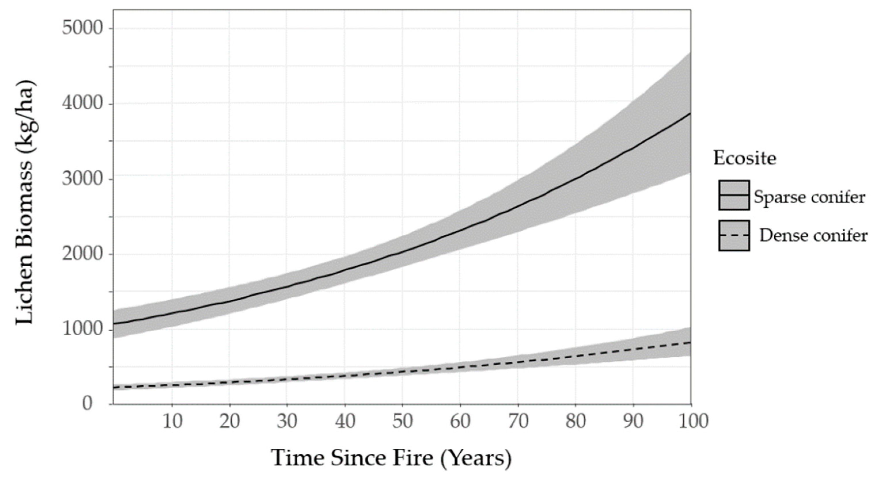
We mapped lichen biomass across Woodland Caribou Provincial Park using a spatial modelling approach that can provide a framework to generate lichen biomass maps for resource management and ecological research in Canada’s boreal forest. By relating our field observations of lichen abundance to forest structure, topographic and remote sensing attributes, we were able to identify environmental features useful in predicting ground lichens. We found that time-since-fire and ecosite were important predictors of ground lichens. 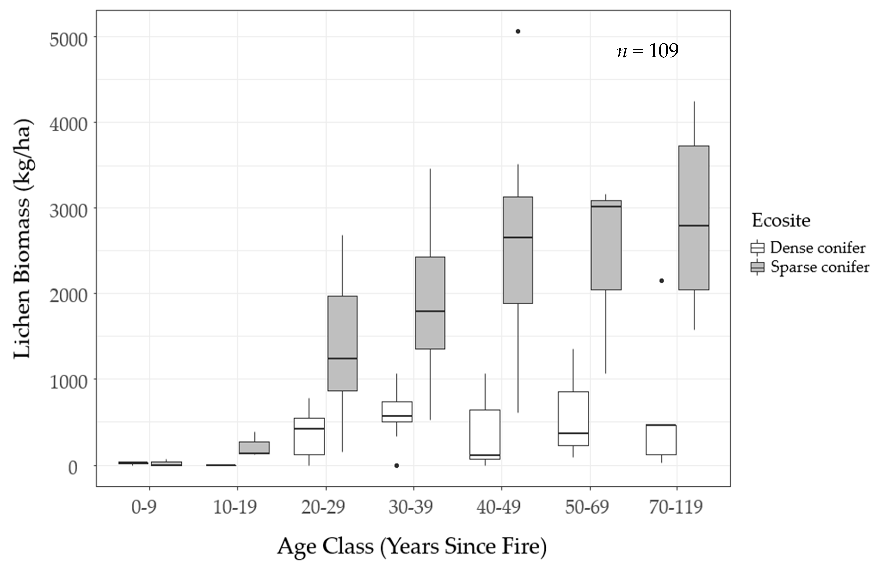Probability of occurrence and biomass of ground lichens was negatively associated with dense conifer ecosites (Table 5, Table 7) and such stands demonstrated low lichen abundance (<1000 kg/ha) across the local time-since-fire continuum (Figure 6). Conversely, sparse conifer ecosites supported very low lichen abundance in the first 20 years after fire, but lichen biomass increased steadily from 20–50 years post-fire (Figure 5). Mature sparse conifer (≥ 70 years old) supported approximately three times more lichen biomass than dense conifer of the same age (Figure 6).

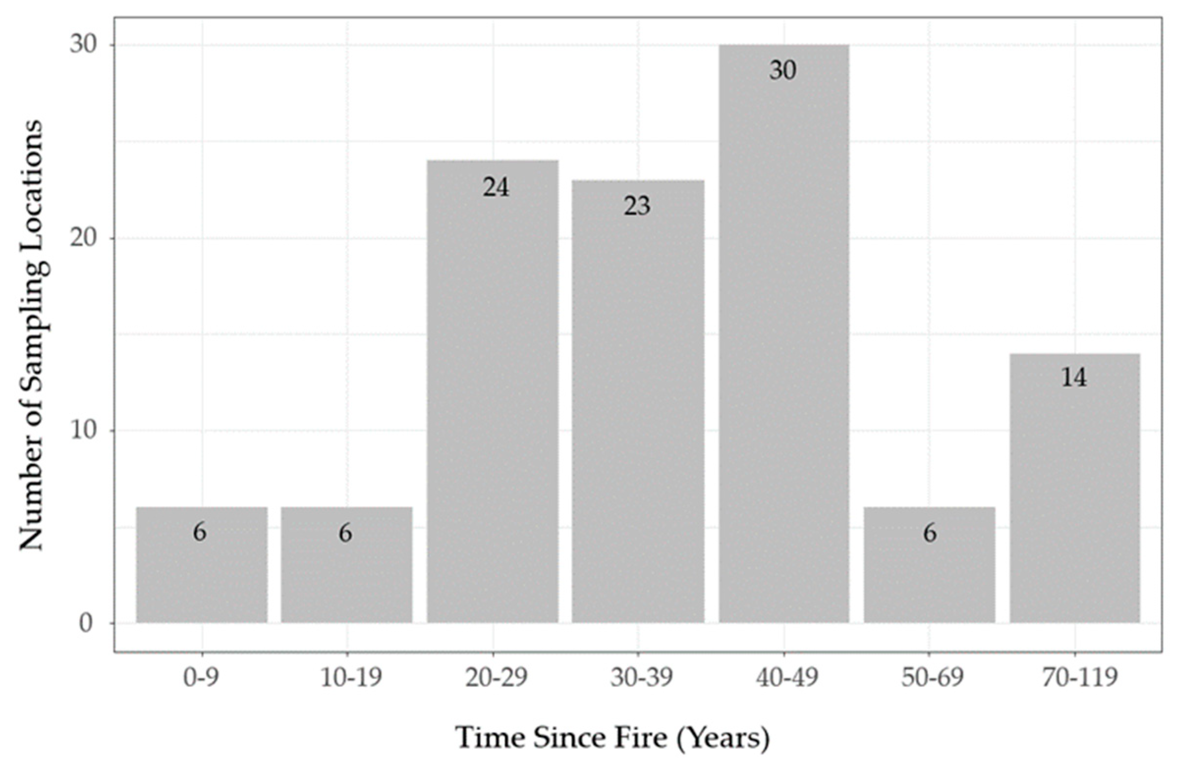
The lichen abundance model appears to overestimate lichen biomass in young sparse conifer stands (0−19 years post-fire; Figure 6) relative to what was observed in the field (Figure 5). Similarly, the model appears to exaggerate the accumulation of lichen biomass in older stands (≥ 50 years old). These discrepancies could be due to the unbalanced sampling design we employed, as we focused most of our sampling effort on middle-aged stands due to a secondary objective to test post-fire lichen recovery. This resulted in few observations at the young (0−19 years post-fire, n = 12) and older (50−119 years post-fire, n = 20) portions of the local post-fire continuum (Figure 3). In addition, our field observations suggest lichen biomass may follow a non-linear pattern with time-since-fire in sparse conifer ecosites (Figure 5). We were unable to fully capture this trend in our analysis because generalized linear models assume a linear relationship between the response variable and the predictor variables. Other model types such as generalized additive models can improve predictions of non-linear trends [46]. Species distribution models [46] such as those developed through MaxEnt [49], provide a highly flexible workflow for mapping the distribution of plants, and have been used to map the presence of lichens [50]. Future research could incorporate these approaches to generate lichen maps for caribou conservation.

In our study, lichen presence was positively associated with canopy closure (Table 5). Conversely, lichen biomass was negatively associated with canopy closure (Table 7). Lichen growth is typically maximized at intermediate levels of canopy closure (~40%) [51], beyond which the growth of mosses is promoted at the expense of lichens [6]. Thus, lichens may require a minimum amount canopy closure to be present at a site but experience reduced growth at high levels of canopy closure, perhaps explaining the opposing responses of lichen presence and biomass observed here. In the oldest stands we sampled (70−119 years old), high mortality of mature trees created large gaps in the canopy and increased sun exposure at ground level. This promoted the growth of juniper shrubs (Juniperus communis L.), which often covered the ground lichens, possibly reducing access to foraging caribou. We had limited observations in overmature conifer stands (n = 14) and suggest future work should measure lichen biomass and caribou habitat selection in mature (50−70 years old) and overmature stands (≥70 years old) to estimate the optimal renewal period for caribou habitat. This information is essential to develop effective fire response and resource management plans that consider caribou conservation.

Most previous studies quantifying lichen over large areas only used remote sensing [9,18,21,22] or environmental [13,14] data. We anticipated that combining forest structure and topographic attributes with remote sensing attributes would provide the best results. Contrary to our expectations, models with only forest structure and/or topographic attributes were just as predictive as models including remote sensing attributes. The candidate models for both lichen presence and lichen abundance had small differences between AICc scores (∆AIC_C < 2) (Table 4; Table 6), which would typically indicate support for multiple candidate models [52]. However, the best candidate model for lichen presence and lichen abundance was the base model, the most parsimonious of the candidate set, only containing ecosite (i.e., dense conifer vs. sparse conifer), time-since-fire and canopy closure as covariates. The penalty weight assigned by AIC_c to more complex models [52] indicates that the additional topographic and remote sensing covariates did not improve explanatory power over the base model.

The lack of support for candidate models with remote sensing covariates could arise from multiple sources. First, environmental and remote sensing covariates are often correlated. We controlled for collinearity within models but, because we were interested in predicting lichen abundance rather than inferring ecological relationships, we did not account for correlation amongst models. Second, the coarse spatial resolution of Landsat imagery can cause trees to mask the spectral signature of ground lichens [14]. Keim et al. (2017) [9] report an R² = 0.74 for a lichen map generated using QuickBird satellite imagery (2.5 m pixels) and LiDAR data (1 m pixels). They found that QuickBird imagery predicted lichens better than SPOT (6 m pixels) and Landsat (30 m pixels) imagery in their study area in the continuous boreal forest of northeastern Alberta [9]. We suggest that the continued incorporation of finer resolution satellite [9] or UAV imagery [53] may help improve the accuracy of lichen mapping in years to come.

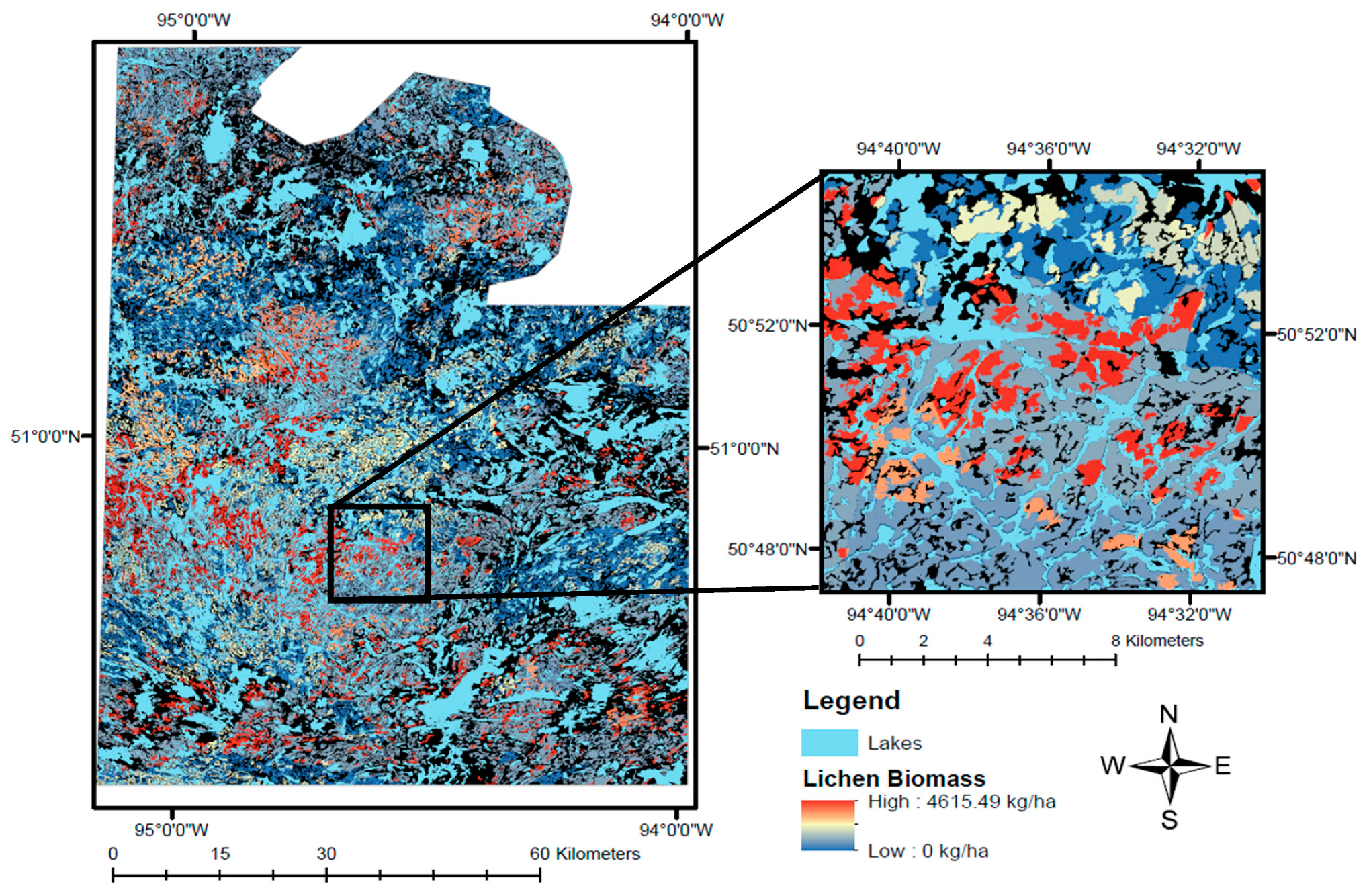
The lichen abundance map we generated in this study (Figure 7) highlights the patchy distribution of lichens on the landscape, which is driven primarily by the prevalence of fire in the study area. Lichen-rich forest is relatively restricted on the landscape, only occurring in mature, sparse conifer ecosites (≥50 years post-fire), where biomass often exceeds 3000 kg/ha (Figure 5). Historically, many researchers used habitat type as a proxy for lichen abundance [54,55,56]. However, some studies have explicitly measured lichen availability and suggest caribou preferentially select stands with ≥3000 kg/ha of ground lichens as winter habitat [8,57,58]. Given that animal nutrition is necessarily related to the amount of available food, ecologists and land managers should strive to understand caribou’s use of lichen biomass across time and space. In particular, identifying the use of lichen biomass during different seasons could be used to delineate nutritionally important habitat patches.

The relatively low accuracy of our map (R² = 0.39) is unsurprising given we used relatively coarse spatial covariates (30 m pixels) to model the presence and abundance of lichens, which are responding to environmental conditions at a very small scale (i.e., microsite). However, we feel that our lichen map provides a reasonable estimation of lichen biomass across our study area and suggest our modelling approach provides a useful framework for researchers to apply and improve in future lichen mapping projects. Most previous research mapped lichen cover [9,13,18], but we suggest lichen biomass is more biologically relevant than lichen cover as biomass is more closely related to animal energetics and fitness [26]. We stress the importance of validating biomass conversion factors and landscape covariates for new study areas, as growing conditions for lichen may vary. For example, in northern Alberta, peatlands are a dominant landscape feature. Previous studies indicate peatlands support much lower lichen abundance than upland sites [35], however raised ‘islands’ of drier peat within bogs can provide better conditions for lichen growth and support locally abundant ground lichens [9,11]. In other parts of the boreal forest, sandy areas dominated by jack pine support thick mats of ground lichens [33]. Integrating abiotic information, such as substrate type, groundwater depth and terrain ruggedness into spatial models may improve lichen predictive mapping, especially when the study area spans multiple biophysical regions. We incorporated data from numerous sources, data types and spatial resolutions to map the abundance of lichens in our study (Table 2). Researchers must be cognizant of the vintage of the source data in each layer they incorporate in their modelling framework to ensure temporal consistency. We suggest future research should focus on incorporating multiple sources of information, including time-since-fire and attributes derived from high resolution satellite imagery (e.g., spectral values, landcover type, forest structure [59]). This will improve spatio-temporal consistency and repeatability. We also encourage researchers to ensure they are selecting the most appropriate model for predicting the distribution of lichens and suggest utilizing generalized additive models [48] may be of particular utility to address some of the deficiencies of this study. Once a lichen abundance map has been generated, we encourage researchers to conduct independent validation using additional field sampling to improve certainty in their spatial predictions.

5. Conclusions

In this study, we propose a modelling framework for predicting the abundance of ground lichens in the boreal forest. We show that ecosite, time-since-fire and canopy closure are important drivers of lichen presence and abundance. We encourage researchers to use and improve our modelling framework to generate spatial predictions of lichen across caribou ranges. There is an increasing emphasis in wildlife ecology on including more biologically relevant variables in habitat selection analyses [60]. Quantifying nutritional landscapes can help researchers and managers measure how food availability changes with succession and varies by habitat type. Explicitly measuring selection for forage abundance can aid in the identification of high-quality habitat and to ensure continuous availability through resource planning and fire response. Mapping forage resources can also be used to test hypotheses, such as the effect of forage abundance on fitness or the tradeoff between nutrition and predator avoidance. Lichen abundance maps should be applied by researchers to help improve our understanding of caribou foraging ecology and support better conservation and resource management decisions.

References

1. Rettie, J.W.; Messier, F. Hierarchical habitat selection by woodland caribou: Its relationship to limiting factors. Ecography 2000, 23, 466–478. [Google Scholar] [CrossRef]
2. Storeheier, P.V.; Mathiesen, S.D.; Tyler, N.J.C.; Olsen, M.A. Nutritive value of terricolous lichens for reindeer in winter. Lichenologist 2002, 34, 247–257. [Google Scholar] [CrossRef]
3. Thompson, I.D.; Wiebe, P.A.; Mallon, E.; Rodgers, A.R.; Fryxell, J.M.; Baker, J.A.; Reid, D. Factors influencing the seasonal diet selection of woodland caribou (Rangifer tarandus caribou) in boreal forests in Ontario. Can. J. Zool. 2015, 93, 87–98. [Google Scholar] [CrossRef]
4. Palo, T.R. Usnic acid, a secondary metabolite of lichens and its effects on in vitro digestibility in reindeer. Rangifer 1993, 13, 39–43. [Google Scholar] [CrossRef]
5. Schaefer, J.A.; Pruitt, W.O. Fire and woodland caribou in southeastern Manitoba. Wildl. Monogr. 1991, 116, 3–39. [Google Scholar]
6. Morneau, C.; Payette, S. Postfire lichen-spruce woodland recovery at the limit of the boreal forest in northern Quebec. Can. J. Bot. 1989, 67, 2770–2782. [Google Scholar] [CrossRef]
7. Carroll, S.B.; Bliss, L.C. Jack pine-lichen woodland on sandy soils in northern Saskatchewan and northeastern Alberta. Can. J. Bot. 1982, 60, 2270–2282. [Google Scholar] [CrossRef]
8. Joly, K.; Chapin, S.F.; Klein, D.R. Winter habitat selection by caribou in relation to lichen abundance, wildfires, grazing, and landscape characteristics in northwestern Alaska. Ecoscience 2010, 17, 321–333. [Google Scholar] [CrossRef]
9. Keim, J.L.; DeWitt, P.D.; Fitzpatrick, J.J.; Jenni, N.S. Estimating plant abundance using inflated beta distributions: Applied learnings from a lichen-caribou system. Ecol. Evolut. 2017, 7, 486–493. [Google Scholar] [CrossRef]
10. Antoniak, K.; Cumming, H.G. Analysis of forest stands used by wintering caribou in Ontario. Rangifer 1998, 18, 157–168. [Google Scholar] [CrossRef]
11. Bradshaw, C.J.A.; Hebert, D.M.; Rippin, A.B.; Boutin, S. Winter peatland habitat selection by woodland caribou in northeastern Alberta. Can. J. Zool. 1995, 73, 1567–1574. [Google Scholar] [CrossRef]
12. Ontario Ministry of Natural Resources and Forestry. Ecosites of Ontario: Boreal Ecosite Factsheets; Ontario Ministry of Natural Resources and Forestry, Ecological Land Classification Working Group: Sault Ste Marie, ON, Canada, 2014. [Google Scholar]
13. Boan, J.; McLaren, B.E.; Malcolm, J.R. Predicting non-inventoried forest elements using forest inventory data: The case of winter forage for woodland caribou. Ecoscience 2013, 20, 101–111. [Google Scholar] [CrossRef]
14. Lesmerises, R.; Ouellet, J.-P.; St-Laurent, M.-H. Assessing terrestrial lichen biomass using ecoforest maps: A suitable approach to plan conservation areas for forest-dwelling caribou. Can. J. For. Res. 2011, 41, 632–642. [Google Scholar] [CrossRef]
15. Uboni, A.; Blochel, A.; Kodnik, D.; Moen, J. Modelling occurrence and status of mat-forming lichens in boreal forests to assess the past and current quality of reindeer winter pastures. Ecol. Ind. 2019, 96, 99–106. [Google Scholar] [CrossRef]
16. Kwok, R. Ecology’s remote-sensing revolution. Nature 2018, 556, 137–138. [Google Scholar] [CrossRef]
17. Wulder, M.A.; Masek, J.G.; Cohen, W.B.; Loveland, T.R.; Woodcock, C.E. Opening the archive: How free data has enabled the science and monitoring promise of Landsat. Remote Sens. Environ. 2012, 122, 2–10. [Google Scholar] [CrossRef]
18. Nelson, P.R.; Roland, C.; Macander, M.J.; McCune, B. Detecting continuous lichen abundance for mapping winter caribou forage at landscape spatial scales. Remote Sens. Environ. 2013, 137, 43–54. [Google Scholar] [CrossRef]
19. Tucker, C.J.; Sellers, P.J. Satellite remote sensing of primary production. Int. J. Remote Sens. 1986, 7, 1395–1416. [Google Scholar] [CrossRef]
20. Wilson, E.H.; Sader, S.A. Detection of forest harvest type using multiple dates of Landsat TM imagery. Remote Sens. Environ. 2002, 80, 385–396. [Google Scholar] [CrossRef]
21. Falldorf, T.; Strand, O.; Panzacchi, M.; Tommervik, H. Estimating lichen volume and reindeer winter pasture quality from Landsat imagery. Remote Sens. Environ. 2014, 140, 573–579. [Google Scholar] [CrossRef] [Green Version]
22. Rickbeil, G.J.M.; Hermosilla, T.; Coops, N.C.; White, J.C.; Wulder, M.A. Estimating changes in lichen mat volume through time and related effects on barren ground caribou (Rangifer tarandus groenlandicus) movement. PLoS ONE 2017, 12, e0172669. [Google Scholar] [CrossRef] [PubMed]
23. Lamb, C.T.; Mowat, G.; McLellan, B.N.; Nielsen, S.E.; Boutin, S. Forbidden fruit: Human settlement and abundant fruit create an ecological trap for an apex carnivore. J. Anim. Ecol. 2017, 86, 55–65. [Google Scholar] [CrossRef] [PubMed]
24. Nielsen, S.E.; Larsen, T.A.; Stenhouse, G.B.; Coogan, S.C.P. Complementary food resources of carnivory and frugivory affect local abundance of an omnivorous carnivore. Oikos 2017, 126, 369–380. [Google Scholar] [CrossRef]
25. Proffitt, K.M.; Hebblewhite, M.; Peters, W.; Hupp, N.; Shamhart, J. Linking landscape-scale differences in forage to ungulate nutritional ecology. Ecol. Appl. 2016, 26, 2156–2174. [Google Scholar] [CrossRef] [PubMed]
26. Avgar, T.; Baker, J.A.; Brown, G.S.; Hagens, J.S.; Kittle, A.M.; Mallon, E.E.; McGreer, M.T.; Mosser, A.; Newmatser, S.G.; Patterson, B.R.; et al. Space-use behavior of woodland caribou based on a cognitive movement model. J. Anim. Ecol. 2015, 84, 1059–1070. [Google Scholar] [CrossRef] [PubMed]
27. Gaynor, K.M.; Brown, J.S.; Middleton, A.D.; Power, M.E.; Brashares, J.S. Landscapes of fear: Spatial patterns of risk perception and response. Trends Ecol. Evolut. 2019, 34, 355–368. [Google Scholar] [CrossRef]
28. Ontario Ministry of Natural Resources. Woodland Caribou Signature Site- Background Information; Ontario Ministry of Natural Resources: Red Lake, ON, Canada, 2004. [Google Scholar]
29. Parks Canada: World heritage sites in Canada- Pimachiowin Aki, Manitoba and Ontario. Available online: https://www.pc.gc.ca/en/culture/spm-whs/sites-canada/sec02s (accessed on 23 June 2019).
30. Carr, N.L.; Rodgers, A.R.; Walshe, S.C. Caribou nursery site habitat characteristics in two northern Ontario parks. Rangifer 2007, 17, 167–179. [Google Scholar] [CrossRef]
31. Bolton, D.K.; Coops, N.C.; Hermosilla, T.; Wulder, M.A.; White, J.C.; Ferster, C.J. Uncovering regional variability in disturbance trends between parks and greater park ecosystems across Canada (1985–2015). Sci. Rep. 2019, 9, 1323–1332. [Google Scholar] [CrossRef]
32. Environment Canada. Recovery Strategy for the Woodland Caribou (Rangifer tarandus caribou), Boreal population, in Canada; Species at Risk Act Recovery Strategy Series; Environment Canada: Ottawa, ON, Canada, 2012. [Google Scholar]
33. McMullin, T.R.; Thompson, I.D.; Lacey, B.W.; Newmaster, S.G. Estimating the biomass of woodland caribou forage lichens. Can. J. For. Res. 2011, 41, 1961–1969. [Google Scholar] [CrossRef]
34. Mallon, E.E.; Turetsky, M.R.; Thompson, I.D.; Fryxell, J.M.; Wiebe, P.A. Effects of disturbance on understory succession in upland and lowland boreal forests and implications for woodland caribou (Rangifer tarandus caribou). For. Ecol. Manag. 2016, 364, 17–26. [Google Scholar] [CrossRef]
35. Dunford, J.S.; McLoughlin, P.D.; Dalerum, F.; Boutin, S. Lichen abundance in the peatlands of northern Alberta: Implications for boreal caribou. Ecoscience 2006, 13, 469–474. [Google Scholar] [CrossRef]
36. Environmental Systems Research Institute (ESRI). ArcMap 10.5.1; ESRI: Redlands, CA, USA, 2017. [Google Scholar]
37. Hijmans, R.J. Raster: Geographic Data Analysis and Modeling. Available online: https://cran.r-project.org/web/packages/raster/index.html (accessed on 9 October 2019).
38. R Core Team. R: A Language and Environment for Statistical Computing. R Foundation for Statistical Computing, Vienna, Austria. 2019. Available online: https://www.r-project.org/ (accessed on 16 October 2019).
39. Ontario Ministry of Natural Resources and Forestry. Forest Resources Inventory (FIM v2 2D) Packaged Product: Kenora Forest, Red Lake Forest, Whiskey Jack, and Woodland Caribou Provincial Park. Available online: https://geohub.lio.gov.on.ca/ (accessed on 9 October 2019).
40. Ontario Ministry of Natural Resources and Forestry. FiresByDecade. Available online: https://geohub.lio.gov.on.ca/ (accessed on 9 October 2019).
41. Aviation, Forest Fire & Emergency Services. Fire Disturbance Area. Available online: https://geohub.lio.gov.on.ca/ (accessed on 9 October 2019).
42. United States Geological Survey. Landsat Surface Reflectance dataset: LC08_L1TP_029024_20140731_20170304_01_T1. Available online: https://earthexplorer.usgs.gov/ (accessed on 9 October 2019).
43. United States Geological Survey. Landsat Surface Reflectance dataset: LC08_L1TP_029025_20140731_20170304_01_T1. Available online: https://earthe×plorer.usgs.gov/ (accessed on 9 October 2019).
44. Ontario Ministry of Natural Resources and Forestry. Provincial Digital Elevation Model (North). Available online: https://geohub.lio.gov.on.ca/ (accessed on 9 October 2019).
45. Hurvich, C.M.; Tsai, C. Regression and time series model selection in small samples. Biometrika 1989, 76, 297–307. [Google Scholar] [CrossRef]
46. Elith, J.; Leathwick, J.R. Species distribution models: Ecological e×planation and prediction across space and time. Ann. Rev. Ecol. Evolut. Syst. 2009, 40, 677–697. [Google Scholar] [CrossRef]
47. Liu, C.; Berry, P.M.; Dawson, T.P.; Pearson, R.G. Selecting thresholds of occurrence in the prediction of species distributions. Ecography 2005, 28, 385–393. [Google Scholar] [CrossRef]
48. Swets, J.A. Measuring the accuracy of diagnostic systems. Science 1988, 240, 1285–1293. [Google Scholar] [CrossRef] [PubMed]
49. Merow, C.; Smith, M.J.; Silander, J.A., Jr. A practical guide to Ma×Ent for modeling species’ distributions: What it does, and why its inputs and settings matter. Ecography 2013, 36, 1058–1069. [Google Scholar] [CrossRef]
50. Allen, J.L.; Lendemer, J.C. Climate change impacts on endemic, high-elevation lichens in a biodiversity hotspot. Biodivers. Conf. 2016, 25, 555–568. [Google Scholar] [CrossRef]
51. Cabrajic, A.V.J.; Moen, J.; Palmqvist, K. Predicting growth of mat-forming lichens on a landscape scale- comparing models with different comple×ities. Ecography 2010, 33, 949–960. [Google Scholar] [CrossRef]
52. Burnham, K.P.; Anderson, D.R. Model Selection and Multi-Model Inference: A Practical Information Theoretic Approach; Springer: New York City, NY, USA, 2002; 515p. [Google Scholar]
53. Fraser, R.H.; Olthof, I.; Lantz, T.C.; Schmitt, C. UAV photogrammetry for mapping vegetation in the low-Arctic. Arct. Sci. 2016, 2, 79–102. [Google Scholar] [CrossRef] [Green Version]
54. Courbin, N.; Fortin, D.; Dussault, C.; Courtois, R. Landscape management for woodland caribou: The protection of forest blocks influences wolf-caribou co-occurrence. Land. Ecol. 2009, 24, 1375–1388. [Google Scholar] [CrossRef]
55. Basille, M.; Fortin, D.; Dussault, C.; Bastille-Rousseau, G.; Ouellet, J.P.; Courtois, R. Plastic response of fearful prey to the spatiotemporal dynamics of predator distribution. Ecology 2015, 96, 2622–2631. [Google Scholar] [CrossRef] [PubMed] [Green Version]
56. Mason, T.H.E.; Fortin, D. Functional responses in animal movement e×plain spatial heterogeneity in animal-habitat relationships. J. Anim. Ecol. 2017, 86, 960–971. [Google Scholar] [CrossRef] [PubMed]
57. Johnson, C.J.; Parker, K.L.; Heard, D.C. Foraging across a variable landscape: Behavioral decisions made by woodland caribou at multiple spatial scales. Oecologia 2001, 127, 590–602. [Google Scholar] [CrossRef] [PubMed]
58. Trudell, J.; White, R.G. The effect of forest structure and availability on food intake, biting rate, bite size and daily eating time of reindeer. J. Appl. Ecol. 1981, 18, 63–81. [Google Scholar] [CrossRef]
59. Matasci, G.; Hermosilla, T.; Wulder, M.A.; White, J.C.; Coops, N.C.; Hobart, G.W.; Zald, H.S.J. Large-area mapping of Candian boreal forest cover, height, biomass and other structural attributes using Landsat composites and lidar plots. Remote Sens. Environ. 2018, 209, 90–106. [Google Scholar] [CrossRef]
60. Hebblewhite, M.; Haydon, D.T. Distinguishing technology from biology: A critical review of the use of GPS telemetry data in ecology. Phil. Trans. R. Soc. B 2010, 365, 2303–2312. [Google Scholar] [CrossRef]
61. Ontario Ministry of Natural Resources: Forest Information Manual 2009: Forest Resources Inventory Technical Specifications. Available online: https://www.ontario.ca/document/forest-resources-inventory-technical-specifications (accessed on 10 October 2019).
Figure 1. Location of the study area in northwestern Ontario, Canada. Sampling locations, indicated by red dots, are concentrated in and around Woodland Caribou Provincial Park, west of the town of Red Lake.
Forests 10 00962 g001
Figure 2. Framework used to generate a lichen biomass map for Woodland Caribou Provincial Park, Ontario, Canada.
Forests 10 00962 g002
Figure 3. Distribution of sampling locations used to quantify lichen abundance across the local time-since-fire continuum in Woodland Caribou Provincial Park, Ontario, Canada (n = 109).
Forests 10 00962 g003
Figure 4. Field sampling protocol used to conduct vegetation surveys in a 12-year-old burn in Woodland Caribou Provincial Park, Ontario, Canada. Sampling was limited to dense conifer (dark green) and sparse conifer (light green) ecosites. Unsampled ecosites are coloured brown, lakes are coloured blue. Sampling locations (red dots) were marked by a GPS waypoint at the 25 m mark of the transect. The 50 m transect is represented by a black line and 1 m² quadrats are represented by open circles (right panel).
Forests 10 00962 g004
Figure 5. Estimated stand-level lichen biomass (kg/ha) by decadal time-since-fire class in dense conifer (white boxplots) and sparse conifer (gray boxplots) ecosites sampled in Woodland Caribou Provincial Park, Ontario, Canada. The thick black line is the median.
Forests 10 00962 g005
Figure 6. Lichen biomass (kg/ha) in sparse conifer and dense conifer ecosites as time-since-fire increases. Simulated from the top lichen abundance model for Woodland Caribou Provincial Park, Ontario, Canada. The dark lines represent the average trendline for each ecosite and the grey banners represent standard errors.
Forests 10 00962 g006
Figure 7. The lichen biomass raster generated for Woodland Caribou Provincial Park, Ontario, Canada. The left panel of the figure shows the entire extent, the right panel shows a close-up of the area around Mexican Hat Lake in the southeast corner of Woodland Caribou Provincial Park. Pixel values represent lichen biomass (kg/ha) from low (blue) to high (red) in dense conifer and sparse conifer ecosites. Lakes appear in light blue. Unsampled ecosites (NoData; Appendix C) are coloured black.
Forests 10 00962 g007