Abstract
Ochroma pyramidale (Cav. ex. Lam.) Urb. (balsa-tree) is a commercially important tree species that ranges from Mexico to northern Brazil. Due to its low weight and mechanical endurance, the wood is particularly well-suited for wind turbine blades, sporting equipment, boats and aircrafts; as such, it is in high market demand and plays an important role in many regional economies. This tree species is also well-known to exhibit a high degree of variation in growth. Researchers interested in modeling the height–diameter relationship typically resort to using ordinary least squares (OLS) to fit linear models; however, this method is known to suffer from sensitivity to outliers. Given the latter, the application of these models may yield potentially biased tree height estimates. The use of robust regression with iteratively reweighted least squares (IRLS) has been proposed as an alternative to mitigate the influence of outliers. This study aims to improve the modeling of height–diameter relationships of tree species with high growth variation, by using robust regressions with IRLS for data-sets stratified by site-index and age-classes. We implement a split sample approach to assess the model performance using data from Ecuador’s continuous forest inventory (n = 32,279 trees). A sensitivity analysis of six outlier scenarios is also conducted using a subsample of the former (n = 26). Our results indicate that IRLS regression methods can give unbiased height predictions. At face value, the sensitivity analysis indicates that OLS performs better in terms of standard error of estimate. However, we found that OLS suffers from skewed residual distributions (i.e., unreliable estimations); conversely, IRLS seems to be less affected by this source of bias and the fitted parameters indicate lower standard errors. Overall, we recommend using robust regression methods with IRLS to produce consistent height predictions for O. pyramidale and other tree species showing high growth variation.
1. Introduction
Ochroma pyramidale (Cav. ex. Lam.) Urb. (balsa-tree) is a large Malvaceae pioneer tree species native from tropical forests. This species can reach 30–40 m in height, 60–120 cm in diameter at breast height (DBH), and crowns up to 40 m at the age of 15 years. O. pyramidale is popularly known as balsa-tree and balsa-wood, with natural distribution throughout America, from southern Mexico to Bolivia, northern Brazil and the Antilles [1,2].
Due to its low weight (the density ranges between 0.06 and 0.38 g cm−3) and mechanical resistance, the wood of O. pyramidale is commonly used in wind turbine propellers, sports equipment, ships, and aircrafts [3]. Balsa-wood has been in high demand on the international market, mainly Europe, China, and United States. Therefore, the species is planted in commercial reforestation programs and in mixed plantations to restorage degraded areas [2,4,5].
This species is characterized by high growth rates and is managed in a clear-cutting and replanting system with harvesting of three- to five-year-old stands [5,6]. However, the fast growth contributes to considerable tree diameter and height variability in even-aged stands. The latter is largely due to high competition for water, light and nutrient resources among neighboring trees of similar age [7]. Other important factors such as genetic characteristics, edaphoclimatic conditions, as well as forest management practices may contribute to growth variability; these also have been reported for Eucalyptus spp. (eucalypts) stands, another species with high growth rates [8].
Regarding the management of O. pyramidale stands a lack of practical information exists about the behavior of height–diameter relationships on different site-index classes. The stand dynamics and individual tree characteristics are tightly linked to site-index conditions (local yield-capacity) [9]. O. pyramidale stands management needs reliable information to assess its development [5,6].
The height–diameter relationship involves two very important variables in forest allometrics and modeling. This relationship is not only used to characterize the vertical structure but is also fundamental for many growth and production models [10]. Due to the costs of measuring all tree heights, it is common to use statistical models to describe the height–diameter relationship [6,11,12], which may be performed by site-index and/or age classes to improve predictions.
Ordinary least squares (OLS) is the most widely used estimation method for linear statistical models. However, this method is sensitive to outliers, in which a single atypical value may influence model fits and predictions [13]. In this context and considering that O. pyramidale data may present high variability, it is necessary to consider other regression methods that minimize the influence of outliers.
As concerns OLS regression methods, Montgomery et al. [14] emphasize the importance of the distribution of values in relation to the independent variable. Namely, all values in a data-set are given equal weight, however, each value can affect the relationship between the dependent and the independent variables. That is, the slope of an OLS regression can be disproportionally influenced by extreme values of independent variables which are far from the point cloud (i.e., outliers). Given the above, our study is motivated by the need for improved tree height predictions for O. pyramidale given the high probability of outlier occurrence.
The use of robust regressions is widely known to mitigate the influence of outlier observations [15]. The approach was first developed by Huber [16] and improved by Hampel [17] Rousseeuw [18], Yohai [19]; Yohai and Zamar [20], Maronna and Yohai [21], Aelst et al. [22] among others. Over more than half a century of development, several robust estimators have been proposed: maximum likelihood estimator (M), maximum likelihood estimator modified (MM), generalized M-estimators (GM), least median of squares (LMS), least trimmed squares (LTS), scale estimator (S), generalized S-estimates (GS), and robust and efficient weighted least square estimator (REWLSE), each with their particular characteristics [13,15,23]. Here we focus on M-estimators which are characterized by estimation procedures that use likelihood functions to minimize error [16,24].
The fit of the models by robust regression is performed by iteratively reweighted least squares (IRLS), in which weights are applied to the observations through minimization functions, aiming to reduce the influence of outliers, whose residuals do not meet the traditional linear regression assumptions, especially normality [25,26].
Our study uses a large Ecuadorian data-set of O. pyramidale stands (containing outliers; n = 32,279 trees), in order to compare the performance of OLS and IRLS—when modeling height–diameter relationships. We assess model fitness and validate results using a split-sampling strategy. The overall aim is to derive best-modeling-practices to inform researchers and practitioners.
The specific objectives of our study are to: (i) model height–diameter relationship of Ochroma pyramidale stands from Ecuador by site-index and age classes; (ii) compare the model performance of the regression methods using OLS and IRLS with robust M-estimators, by (iii) employing large data-sets for model fitting and validation (Approach 1) and a smaller data-set representing six outlier scenarios (Approach 2), and (iv) examine the result consistency of performed comparisons by the adjusted determination coefficient, the standard error of estimate (SEE%), and graphical residual analysis. We test the hypothesis that robust regressions provide greater accuracy of height–diameter models than OLS by site-index and age classes in O. pyramidale stands.
2. Materials and Methods
We structure the analysis in two distinct approaches: Approach 1 implements a split-sample strategy to first (split one; n = 24,850) assess the modeling fitness of OLS and IRLS (from hereon, all IRLS estimations are assumed to use M-estimators), and then validate these results using a separate sampling split (n = 7429); Approach 2 uses a sub-sample strategy (one plot; n = 26) to conduct a sensitivity analysis of six artificially constructed outlier scenarios by systematically varying the arrangement or positioning of the outlier in order to assess the effects of these arrangements in both OLS and IRLS methods. Note that in Approach 1, we stratify the data-set by age and site-index:
- (i)
- Stratification into age classes. Given the aggregate summary statistics from Table 1 (i.e., ages varied from 1.1 to 4.8 years), we determined that strata should not include ranges greater than one year. Therefore, four age classes were determined.
 Table 1. Descriptive statistics of height–diameter variables in the fit and validation data-sets of Ochroma pyramidale (balsa-tree) stands in Ecuador.
 - (ii)
- Stratification into site-index classes. Similarly, using aggregate results from Table 1 (i.e., dominant heights [hdom] in the plots varied from 8.6 to 36.9 m), we decided on three site-index strata groupings.
2.1. Approach 1
2.1.1. Study Area Characterization and Data Collection
Data collection was performed in O. pyramidale stands located in five provinces of Ecuador: Los Ríos, Cotopaxi, Guayas, Manabí, and Santo Domingo de Tsachilas, owned by PLANTABAL S.A.—3ACOREMATERIALS®. The altitude ranges from 75–500 m a.s.l. and, according to the Holdridge classification, the region is situated in Tropical Dry Forest and Tropical Moist Forest, with 800–3000 mm year−1 precipitation, average annual temperature around 25 °C and average annual air humidity of about 85%, with slightly uneven topography and soils composed mainly of silt and clay and pH around 6.5–7.0 [5,27].
As previously indicated, Approach 1 splits the full sample of 1414 permanent plots and 32,279 trees into two data-sets: the first data-set denoted as fit data-set was used to fit the equations described below (call this fit data-set) and determine which of these is the most representative model by site-index and age classes (i.e., model with the closest fit); the second validation data-set sample aimed at validating the performance of the most representative model (called validation data-set). On all plots the DBH was measured for all trees and the height of a sub-sample of trees. The DBH was measured with a diameter tape at 1.3 m from the ground and recorded in cm, and the height was determined with a Haglöf clinometers and recorded in m.
The fit data-set contains information collected on 1112 permanent plots, with 24,850 trees (1.1–4.8 years old), of which 9348 have paired measurements of DBH and h. The validation data-set contains information on 7429 trees (1.1 to 4.7 years; 302 permanent plots), of which 2429 trees have paired measurements of DBH and h. Figure 1 features a scatter plot which illustrates the data dispersion for both data-sets. The dotted line corresponds to the average trend of the fit data-set, whereas the solid relates to the validation data-set.
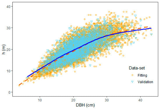
Figure 1.
Dispersion of paired diameter at breast height (DBH) and h data in fit and validation data-sets used to represent the height–diameter relationship (Approach 1).
Figure 2 features the stratification of the fit data-set, by age classes. Visual inspection of this figure highlights noticeable dispersions between DBH and h, along with some possible outliers; it is important to note that such dispersions are visually noticeable in these short one-year periods, with amplitude in height greater than 20 m in all cases.
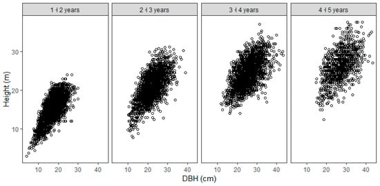
Figure 2.
Dispersion of paired DBH and h data by age classes used to fit models to represent the height–diameter relationship (Approach 1).
Table 1 features descriptive statistics of DBH and h variables for the fit data-set and the validation data-set. The coefficient of variation (cv%) indicates the variability which appears heights in the aggregate rows (labeled ‘all data-set’). Note: some of the rows of validation data-set were intentionally excluded (i.e., stratification by site-index class) given that these were deemed unnecessary as the validation was only performed for the aggregate data (i.e., all data-sets).
2.1.2. Site-Index
The effects of site-index on height–diameter relationship were only assessed for the fit data-set; namely, site-index was only used to assess model fit and not validation. Measurements of dominant height—hdom (m) of the 100 largest trees per hectare were done following Assmann [28]. See Table 2 for descriptive statistics.
Table 2.
Descriptive statistics of variables used in modelling of hdom for Ochroma pyramidale (balsa-tree) stands in Ecuador.
Table 3 details the two statistical models used to predict hdom as a function of age; these were used to determine site-index and the subsequent classification of plots. Model (1) uses linear regression for fit, whereas Model (2) uses non-linear.
Table 3.
Statistical models used to predict dominant height.
The selection criteria used to determine the most representative hdom model is based on: the adjusted determination coefficient (R2adj.); the standard error of estimate in percent (SEE%); along with a graphical analysis of standardized residuals. These measures were also used to determine the most appropriate height–diameter model (more on this below).
For Model (1), we use a logarithmic transformation (Meyer correction factor [MCF]) [31] to correct for the log back-transformation regarding the hdom predicted values (see Equation (1)); more specifically, the following was used to recalculate the SEE%:
where MSE is mean square error.
The corresponding values of the guide curve come from the dominant heights of the 1112 permanent plots (i.e., aggregate fit data-set). Once the most representative model was selected, the guide curve method was used to predict the site-index curves. Three site-index classes were considered based on the amplitude of the hdom data at the reference age (aRef). The aRef was set at 3.5 years since it was close to the O. pyramidale age of clear-cutting and replanting system with harvesting (5.0 years old stand).
2.1.3. Height–Diameter Relationship
Table 4 features the four classic models used to describe the height–diameter relationship. These models were fitted in the following manner in three ways: (i) using the aggregate set of observations (i.e., ‘all data-set model’); (ii) stratifying by age; and (iii) stratifying by site-index. These various model specifications were used to determine the most appropriate method to predict the heights.
Table 4.
Statistical models for estimating total height.
The data were stratified into four age classes (I: 1 ˧ 2 years, II: 2 ˧ 3 years, III: 3 ˧ 4 years and IV: 4 ˧ 5 years) and three site-index classes (I, II e III). In each class, two modeling methods were tested: traditional linear regression with ordinary least squares (OLS) and robust regression by iteratively reweighted least squares (IRLS), in which three maximum likelihood estimators were tested (M-estimators): Huber, Hampel, and Biweigth (Tukey), whose objective and weight functions are described in Table 5.
Table 5.
Functions and condition of maximum likelihood estimators (M-estimators).
According to the condition of each estimator, the value of breakdown point (k) in the case of the Huber and Biweight estimators, and the values of a, b, and c of the Hampel estimator, correspond to the restrictions that determine which weight function is applied to the residuals. In the first case, small values of k penalize more outliers, but reduce accuracy when the residuals are normally distributed. Because of this, it is suggested to apply k = 1.345 which guarantees a loss of efficiency of up to 5% over OLS [13,18,20].
The ranking of the models fitted to represent height–diameter relationship by site-index and age classes was based on their accuracy, for which the relative change of SEE% was quantified by applying both estimation methods (IRLS and OLS).
To verify the linear regression assumptions, Lilliefors’s test (D) with 95% probability level was used to assess normality, as well as the graphic analysis of the residuals using the normal quantile-quantile plot (QQ-plot). To evaluate the homoscedasticity, Breusch-Pagan’s (BP) test [36] with 95% probability level was applied and the standardized residuals graphs were analyzed. The tests were used to examine for violations: given that no violations could be identified, we proceeded to evaluate the significance of the corresponding estimated parameters.
Complementing the analysis, the coefficient of variation (cv%) was calculated and the significance of regression parameters was evaluated by Student’s t-test with 95% probability level. Data processing were performed using R® software, version 3.6.1. [37]—the MASS package for R [38] (with the rlm function) was used to perform robust regression.
In summary, all the above model specifications and tests for assumptions were used to select the most representative model for the aggregate fit data-set (i.e., all data-set) and by site-index and age classes; this fit model for all data was subsequently validated using the validation data-set. Our validation strategy follows [26,39]; as such, a data-set with 2500 observations (~20%) was randomly sampled (from the full data-set), and the adherence between the observed and predicted data was determined by using the Chi-square test (χ²) with 95% probability level; thus, we test the hypothesis that predicted estimates by OLS or IRLS are not different than the observed values. This analysis was complemented with the density histogram performed using the geom_density function of the ggplot2 package [40] of R software [37]. Additionally, the standardized residuals plot was evaluated, and the SEE% was calculated.
It is important to note that all equations featured by this study (i.e., assessed for performance) were validated using data from the same sampling regions of Ecuador. Thus, data for validation were not independent. However, the goal of independent data validation to assess the generalizability of performance of these equations, in other region (or stands), was not the focus of this study. Our contribution, as initially noted, was to demonstrate empirically an improvement to the standard research approach (using OLS with species with high variation). Lastly, we further note that our sampling region contains roughly 80%–90% of all O. pyramidale stands worldwide, therefore, our results carry representative strength in terms of this particular species.
2.2. Approach 2
Approach 2 uses a smaller data-set of O. pyramidale (1 plot test case; n = 26 trees), to conduct a sensitivity analysis which compares the Henriksen’s model (fitted by OLS; henceforth OLS) with the Huber estimator of IRLS (henceforth IRLS).
The raw data from this approach come from 1 permanent plot that was selected from the aggregate fit data-set (1112 plots). This plot includes 26 trees of the same age (4.7 years). We note that the number of trees in this particular plot is slightly higher than the average number of trees-per-plot from the entire sample used in Approach 1 (~22 trees-per-plot).
The following six sensitivity analysis scenarios were artificially constructed: 1 scenario with no outliers (S1); and 5 other scenarios containing two different outliers (S2, S3, S4, S5, and S6; see Figure 3). The artificially created outliers included in scenarios 2–6 were added visually. This visual strategy was guided by two main considerations: (1) the definition of an outlier provided by Montgomery et al. [14]; and (2) the working experience of field teams re-measuring the sample plots.
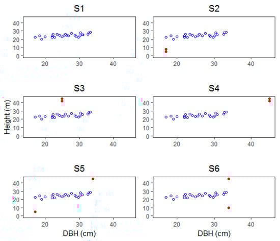
Figure 3.
Sensitivity analysis of 6 scenarios (S1 to S6) from a subsample with 26 trees of the same (4.7 years), 5 scenarios containing artificially created outliers (Approach 2) for modeling of height–diameter relationship of O. pyramidale in Ecuador.
Montgomery et al. [14] describe similar scenarios; the authors also note that such situations (similar to Figure 3) occur fairly often in practice, adding that, in general, researchers should be aware that in some data-sets, one point (or a small cluster of points) may influence key modeling properties.
These scenarios were artificially developed in order to examine model performance using typical outlier observations that could be found in forest allometric databases; the capacity to control for the placement of these also simplified the analysis which enables the understanding the specific objectives of this research (i.e., difference between (OLS and IRLS).
3. Results
3.1. Approach 1
3.1.1. Site-Index
According to the fit statistics evaluated, the Champan–Richards’ model (2) in Table 3 was selected to describe the behavior of hdom, which presented R2adj. = 0.709 and SEE% = 12.71%. The regression parameters for Equation (2) were significant (p < 0.01).
Graphical analysis of the residuals (Figure 4a) shows that most of them are distributed between −2 to 2 standard deviations along the predicted line. The site-index curves from Equation (2) (Figure 4b) allowed to classify all plots in different classes, resulting in 33.7% in site-index class I, 48.1% in class II and 18.2% in class III.
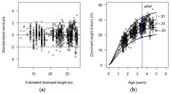
Figure 4.
Standardized residuals for predicted hdom (a) and site-index curves (b) for Ochroma pyramidale (balsa-tree) stands in Ecuador.
3.1.2. Height–Diameter Relationship
The most representative height–diameter models fitted by site-index and age classes are presented in Table 6. Näslund’s model presented better fit in site-index classes and all data-set through robust regression using Biweight estimator. For age classes, Curtis’s model appears to offer the closest fit (as compared to the observed data), this is followed by Henriksen; however, its fits were better through OLS method, except for class III, where IRLS was more statistically accurate with Hampel’s estimator.
Table 6.
Statistics of the most representative fit models for estimating the total height of Ochroma pyramidale (balsa-tree) trees by site-index and age classes in Ecuador.
The stratified model results for site-index classes indicate that SEE% reduces in smaller classifications (goes from 0.3084% to 0.4481%)—this applies to models fitted by IRLS with the Biweight estimator in comparison with the OLS estimator (Table 6). In the fits by age classes there was better accuracy by the OLS method, except for class IV, where the reduction in SEE% of 0.0018% was observed by applying robust regression through Hampel’s estimator.
The regression parameters and their respective standard errors of the most representative height–diameter models fitted by site-index and age classes are shown in Table 7, in which they were significant (p < 0.05).
Table 7.
Parameters standard errors of the most representative fit models for estimating the total height of Ochroma pyramidale (balsa-tree) trees by site-index and age classes in Ecuador.
Approach 1 presented relative difference between standard errors by OLS and IRLS less than 3% (Table 7). The negative percentage values in dif. S.E. indicate that the regression parameters standard error by IRLS was higher than OLS.
The quality of fit and consequently the predictions by classes of site-index and age were graphically verified (Figure 5). Data stratification resulted in homogeneous distribution of observations, where the best site-index (I) and the highest age (IV) presented the highest total tree heights.
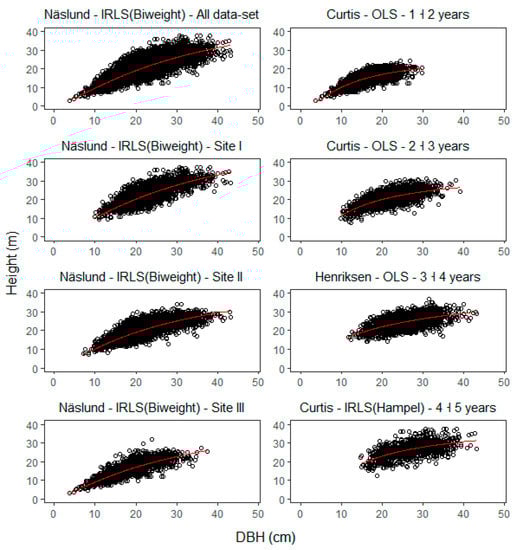
Figure 5.
Predicted curves for the most representative model by classes of site-index and age for Ochroma pyramidale (balsa-tree) stands in Ecuador.
When evaluating the assumptions of the regression analysis, it was observed that, in most cases, the normality of the residuals was rejected by the Lilliefors test (p < 0.05). However, the normal QQ-plot showed that the residuals follow the normal distribution trend, with some outliers on two-tailed (Figure 6).
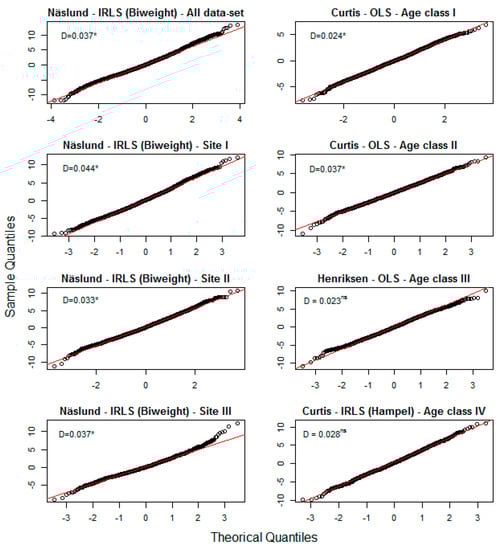
Figure 6.
Graphical analysis of normality for the most representative model fitted by site-index and age classes for Ochroma pyramidale (balsa-tree) stands in Ecuador. D: Lilliefors’ test value. * is statistically significant at p < 0.05, ns is not statistically significant at p < 0.05.
The graphical analysis of residuals of models adjusted by site-index and age classes (Figure 7), does not seem to indicate the presence of a greater bias along the midline. This is in spite of the Breusch–Pagan test rejecting the homogeneity hypothesis in almost all adjustments (p < 0.05), except for age classes III and IV.
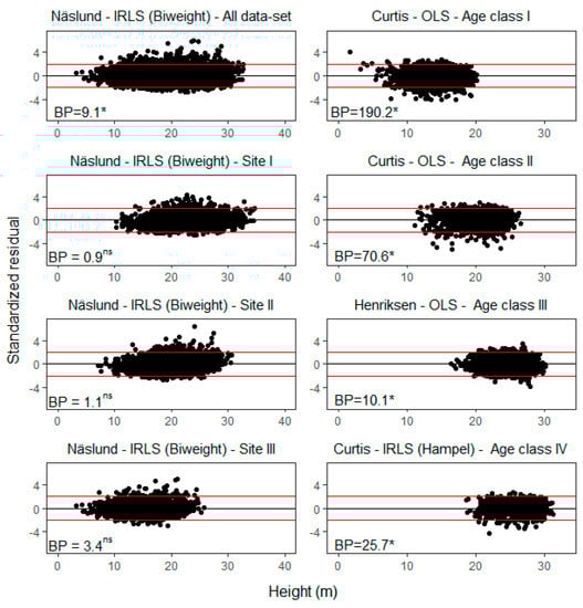
Figure 7.
Standardized residual plot for the most representative models fitted by site-index and age classes for Ochroma pyramidale (balsa-tree) stands in Ecuador. BP: Breusch–Pagan’s test value. * is statistically significant at p < 0.05, ns is not statistically significant at p < 0.05.
The results from the validation data-set confirm the Näslund model adjusted by IRLS (Biweight) as the most representative fitted model for all data-sets (i.e., no stratification). This result can be seen in Figure 8a; namely, the χ2 test did not reveal sufficient evidence to reject the null hypothesis (at the 95% level); furthermore, the SEE% for this model was similar to that obtained in the fit data-set (15.516%). In summary, this appears to show that the equation obtained from the Näslund model adjusted by IRLS (Biweight) can be used to appropriately represent the height–diameter relationship in O. pyramidale using the non-stratified data-set.
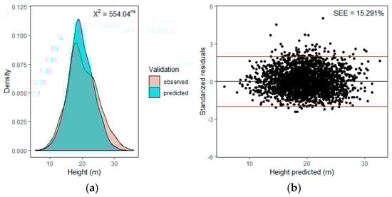
Figure 8.
Density histogram (a) and standardized residuals (b) in the validation. X2: chi-square test; ns: not significant with 95% probability level; SEE%: standard error of estimate in percent.
3.2. Approach 2
Statistics for the Henriksen model fitted by OLS and IRLS (Hampel) in the six scenarios evaluated in this approach are presented in Table 8. In all cases, there were higher values of R2adj. and lower SEE% values using the OLS method. The negative value of R2adj. in scenario 3 is due to the high value of the sum of squares of the residual due to the outlier.
Table 8.
Statistics for Henriksen’s model fitted to predict total height in Ochroma pyramidale trees of age 4.7 in Ecuador (Approach 2).
The parameters of the fitted equations from the Henriksen model for the six scenarios of Approach 2, as well as their standard errors and the difference between them, are shown in Table 9. Except for scenario 1 (without outlier), in all cases the IRLS (Hampel) method resulted in the lowest parameters standard error, whose difference with OLS ranged from 38.11%–82.81%.
Table 9.
Parameters standard errors in the Henriksen’s model fitted to predict total height of O. pyramidale from a subsample of data with 4.7-year-old trees in Ecuador (Approach 2).
In Figure 9, the OLS fit curves are compared with the IRLS fit using the three M-estimators. It is evident in S2 to S6 that the outliers influenced the results, distancing the OLS fitted curves from those fitted by IRLS.
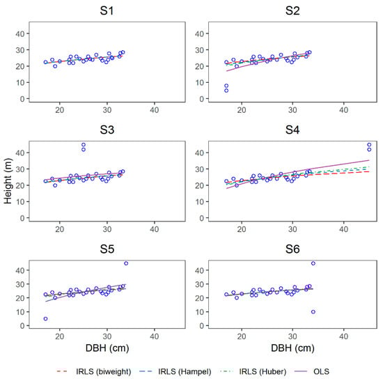
Figure 9.
Predicted curves for the Henriksen’s model fitted for Ochroma pyramidale (balsa-tree) aged 4.7 years in Ecuador for six different scenarios (S1 to S6).
In the evaluation of absolute residuals for Approach 2, it was observed in Figure 10 that in scenarios with outliers, there were biases in S2, S3, S4 and S5 using OLS, something not observed in the residuals generated by IRLS (Hampel) method.
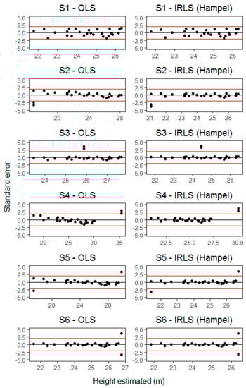
Figure 10.
Residuals of Henriksen’s model fitted for Ochroma pyramidale (balsa-tree) aged 4.7 years in Ecuador for six different scenarios (S1 to S6).
4. Discussion
According to the site-index results for O. pyramidale evaluated in Approach 1, the Chapman–Richards model was the most representative for hdom predicted, although it showed a slight tendency to underestimate at the lowest heights and overestimate at the highest (Figure 4a). Because it is a non-linear biological model with three parameters, it is very flexible and can properly represent the growth of an allometric variable like hdom over time [5,39,41].
Based on the result of R2adj. (0.709) of the Chapman–Richards fitted model, it is possible to state that, in O. pyramidale stands, the independent variable (age) explained the behavior of the dependent variable (hdom) very well. On the other hand, regarding the SEE% (12.71%), although it can be considered high (>10%) [42]), the result was satisfactory for the estimation of hdom in the context of the variability presented by the data (overall cv% 24.3%, Table 2).
It was observed that hdom amplitude over age was greater than 10 m (Figure 4b), which proves to be a feature of the development of O. pyramidale, especially when seminally propagated, in which there is greater genetic variability [43]. Our study does not control for this type of variability in growth; we note that this is a limitation in our study which could influence the way we classified plots in terms of site-index.
Since the site-index curves from Figure 4b do not include all observations, our site-index classification, pertaining to intervals upper-class I and lower-class III, may have been ‘kept open’—as described by Cañadas-López et al. [5].
Through site-index classification, it was possible to group the plots of the study into three productivity classes, with approximately half of them allocated to the intermediate class and the others to the lower and upper classes. This allowed for reducing the variability of observations by class and improving height–diameter predictions. The dominant height of O. pyramidale is closely related to the site-index, as with other species [10,44]. Future work is suggested related to the effects of site-quality, which ideally ought to also account for the effects of climate, soil and forest management.
Results from Approach 1 suggest that DBH growth and h of O. pyramidale is related to site-index and age classes (Figure 5). Our findings also suggest that models that do not stratify are out-performed by models that stratified by age—these results were consistent in both OLS and IRLS. The above provides evidence of a relationship between data variability and fit performance; namely, models that do not stratify and models that only stratify by site-index appear to display a higher percentages of variation (i.e., cv%; see Table 1).
Our results (Table 6) also show better performance in models fitted by IRLS (e.g., Näslund; using Biweight)—this result appears consistent in models that do not stratify and those that only stratify by site-index. These results using the Näslund model are consistent with other empirical studies e.g., [45], which suggests a certain flexibility of this model to describe the height–diameter relationships; namely, the mathematical design of this model appears to allow for better residual distribution—when evaluated directly from a linear model fit that does not isolate for the influence of the variable h (Figure 7).
The higher accuracy of IRLS predictions of data with greater variability is due to the application of lower weights to outliers, minimizing error and improving the quality of fit [24,26,46]. This result appears to be supported by models that stratify for site-index classes and those that do not stratify; namely, these two model specifications appear to exhibit greater variability for h and DBH (cv% >20%, Table 1)—this suggests a relative gain in accuracy (SEE%) when compared to models that stratify by site and age classes (Table 6).
In contrast, the gain in accuracy of OLS models that stratify by age classes appears to be partially explained by the better compliance of regression assumptions and lower variability for h and DBH (cv% <20% in most cases, Table 1). In fact, when the linear regression assumptions are fulfilled, the OLS method enables more accurate predictions than robust estimators [15,18,20,22].
A desirable feature when fitting linear models is the smallest parameter standard error. Table 7, shows for Approach 1 that, in this regard, both fitting methods presented less than 3% difference when analyzing the standard errors in the different classes of site-index and age. This suggests, a priori, that the performance of the four models adjusted by OLS and IRLS is very similar and this reflects the results in SEE% and R2adj. that had little difference.
Regarding the apparent violation, in some cases, of the normality assumption, it was demonstrated for Approach 1 that the residuals of the fitted models follow the typical behavior of a normal distribution (Figure 6) and this proves that OLS performs best in most age classes. On the other hand, robust regression has the characteristic that it can be used even when there is violation of regression assumptions [18,20,22,25,26].
The distribution of standardized residuals (Figure 7) appears to be related to data variability (this result was found in both in DBH and h). This variability seems to account for a portion of bias in the predictions of the height–diameter relationship; this was identified in particular in models that models stratified by age. We note that these models included several observations that were considered outliers (i.e., values with magnitudes greater than 2 standard deviations).
In Approach 2, there was also a similar result of SEE% and R2adj. for the Henriksen model adjusted by both methods in the six scenarios evaluated; however, the IRLS (Hampel estimator) technique allowed a decrease in the parameters standard error from 43.38%–67.41% (Table 9) compared to OLS in extreme scenarios (S2–S6).
Previous results suggest that, although important, the R2adj. and SEE% statistics are not appropriate to compare OLS and IRLS methods with robust M-estimators. The parameter standard error is appropriate to compare the methods since it is directly related to the confidence interval of the predictions, and consequently to the efficiency of the model, which is something that actually differs in the fitting of the two methods.
M-estimators are resistant to outliers in the dependent variable but are sensitive to the high number of leverage points in the independent variable [13]. In this sense and based on the results obtained for Approach 1 by the three M-estimators tested, it was found that the data-set used in modeling the height–diameter relationship by site-index and age classes presents some variation with some possible outliers in both dependent variable h and independent variable DBH (Table 1). This characteristic of the data-set conditions the efficiency of the M-estimators.
Outliers that do not relate to data collection errors should not be removed from the analysis [47]. When outliers are present, robust regression is indicated due to its similar precision with the least squares method; however, the robust regression can decrease the parameter standard error, as demonstrated in the present study and which is directly related to the confidence interval of the predictions. However, in the absence of outliers the loss of efficiency of robust estimators compared to the OLS can be a maximum of 5% [13,18,20].
5. Conclusions
Approach 1 of this study demonstrates the improvements in the modeling of height–diameter relationships, by site-index and age-classes, using a large sample of forest inventory plots in O. pyramidale stands in five Ecuadorian provinces (n = 9348); our findings suggest that non-stratified models are out-performed by models stratified by age-classes. The results suggest consistent performance improvements when using robust regressions with iteratively reweighted least squares—as compared to OLS. Notwithstanding this, we note that there is no single model that represents all the different site-index and age classes, since development in diameter at breast height and total height of this species features high variability over time. In Approach 2, we use a sub-sample of sample tree data (n = 26) to engage in a sensitivity analysis which indicates that IRLS decreases the standard error of regression parameters and improves the confidence of the predicted values.
Robust regression with the M-estimators for models fitted by iteratively weighted least-squares can improve more accurate predictions of the total height of O. pyramidale relative to the ordinary least squares method; these were particularly noted when comparing models which failed past tests of classical linear assumptions, as well as those with a cv% that is greater than 20%.
Furthermore, the performance comparison of the fitted models by both methods, based on the adjusted determination coefficient (R2adj.) and standard error of estimate in percent (SEE%), is not consistent since the results with outliers do not show a clear trend. Thus, the efficiency of these methods can be better analyzed based on the standard errors of regression parameters and the graphic distribution of the residuals.
In summary, the results of this study are timely, given that many practitioners and researchers in the private sector typically use OLS to analyze a relatively small forest operation (i.e., relatively small number of plots). Given the results of this study, we advise researchers who are interested in analyzing data with high variability (particularly those using a relatively small sample size) to consider the benefits of improving estimations using robust methods; namely, our results using large data-sets (i.e., Approach 1) appear to indicate performance parity of robust methods to OLS, whereas Approach 2 shows evidence of performance improvements in the presence of outliers and in smaller data-sets.
Author Contributions
Conceptualization, J.D.Z.-C., J.E.A., A.L.P., A.B. and J.R.S.; methodology, J.D.Z.-C., A.L.P., A.B. and J.R.S.; software, J.D.Z.-C., A.L.P. and G.A.O.; validation, J.D.Z.-C., A.L.P., A.B. and G.A.O.; formal analysis, J.E.A., J.R.S., M.S.G. and R.d.L.E.; investigation, J.D.Z.-C., J.E.A., A.L.P. and A.B.; resources, J.R.S. and M.S.G.; data curation, J.D.Z.-C. and R.d.L.E.; writing—original draft preparation, J.D.Z.-C. and A.L.P.; writing—review and editing, J.E.A., A.B., G.A.O., J.R.S., M.S.G. and R.d.L.E.; visualization, J.D.Z.-C. and G.A.O.; supervision, J.E.A., A.L.P. and A.B.; project administration, J.E.A. and M.S.G.; funding acquisition, J.E.A., M.S.G. and J.R.S. All authors have read and agreed to the published version of the manuscript. Please turn to the CRediT taxonomy for the term explanation. Authorship must be limited to those who have contributed substantially to the work reported.
Funding
This research was funded by the Coordenação de Aperfeiçoamento de Pessoal de Nível Superior—Brasil (CAPES)—Finance Code 001.
Acknowledgments
The authors would like to extend their sincere appreciation to PLANTABAL S.A.—3ACOREMATERIALS® for their support in developing this research.
Conflicts of Interest
The authors declare no conflict of interest.
References
- Stevens, W.D.; Ulloa, C.; Pool, A.; Montiel, O.M. Flora de Nicaragua; Missouri Botanical Garden Press: New York, NY, USA, 2001; Volume 85, pp. 1–943. [Google Scholar]
- Varón, P.T.; Morales-Soto, L. Árboles en la Ciudad de Medellín; de Alcaldía, M., Ed.; Panamericana Formas e Impresos S.A.: Medellín, Colombia, 2016; p. 202. [Google Scholar]
- Borrega, M.; Gibson, L.J. Mechanics of balsa (Ochroma pyramidale) wood. Mech. Mater. 2015, 84, 75–90. [Google Scholar] [CrossRef]
- Lorenzi, H. Árvores Brasileiras: Manual de Identificação e Cultivo de Plantas Arbóreas do Brasil, 5th ed.; Instituto Plantarum-Nova Odessa: São Paulo, Brazil, 2008; Volume 1, p. 65. [Google Scholar]
- Cañadas-López, Á.; Rade-Loor, D.; Siegmund-Schultze, M.; Moreira-Muñoz, G.; Vargas-Hernández, J.J.; Wehenkel, C. Growth and yield models for balsa wood plantations in the coastal lowlands of Ecuador. Forests 2019, 10, 733. [Google Scholar] [CrossRef]
- Cañadas-López, A.; Rade-Loor, D.; Fernández-Cevallos, G.; Dominguez-Andrade, J.M.; Murillo-Hernández, I.; Molina-Hidrovo, C.; Quimiz-Castro, H. Ecuaciones generales de diámetro-altura para Ochroma pyramidale, Región Costa-Ecuador. Bosques Latid. Cero 2016, 6, 1–14. [Google Scholar]
- Knowe, S.A. Effect of competition control treatments on height-age and height-diameter relationships in young Douglas-fir plantations. For. Ecol. Manag. 1994, 67, 101–111. [Google Scholar] [CrossRef]
- Stape, J.L.; Binkley, D.; Ryan, M.G.; Fonseca, S.; Loos, R.A.; Takahashi, E.N.; Silva, C.R.; Silva, S.R.; Hakamada, R.E.; Ferreira, J.M.A.; et al. The Brazil Eucalyptus Potential Productivity Project: Influence of water, nutrients and stand uniformity on wood production. For. Ecol. Manag. 2010, 259, 1684–1694. [Google Scholar] [CrossRef]
- Sharma, R.P.; Vacek, Z.; Vacek, S.; Kučera, M. A Nonlinear Mixed-Effects Height-to-Diameter Ratio Model for Several Tree Species Based on Czech National Forest Inventory Data. Forests 2019, 10, 70. [Google Scholar] [CrossRef]
- Stankova, T.V.; Diéguez-Aranda, U. Height-diameter relationships for Scots pine plantations in Bulgaria: Optimal combination of model type and application. Ann. For. Sci. 2012, 56, 149–163. [Google Scholar]
- Nicoletti, M.F.; Souza, K.; Silvestre, R.; França, M.C.; Rolim, F.A. Relação hipsométrica para Pinus taeda L. em diferentes fases do ciclo de corte. Floram 2016, 23, 80–89. [Google Scholar] [CrossRef][Green Version]
- Stolle, L.; Velozo, D.R.; Corte, A.P.D.; Sanquetta, C.R.; Behling, A. Modelos hipsométricos para um povoamento jovem de Khaya ivorensis A. Chev. BIOFIX Sci. J. 2018, 3, 231–236. [Google Scholar] [CrossRef]
- Yu, C.; Yao, W. Robust linear regression: A review and comparison. Commun. Stat. Simul. Comput. 2017, 46, 6261–6282. [Google Scholar] [CrossRef]
- Montgomery, D.C.; Peck, E.A.; Vining, G.G. Introduction to Linear Regression Analysis, 5th ed.; John Wiley & Sons, Inc.: Hoboken, NJ, USA, 2012; Volume 821, p. 505. [Google Scholar]
- Alma, Ö.G. Comparison of robust regression methods in linear regression. Int. J. Contemp. Math. Sci. 2011, 6, 409–421. [Google Scholar]
- Huber, P.J. Robust version of a location parameter. Ann. Math. Stat. 1964, 35, 73–101. [Google Scholar] [CrossRef]
- Hampel, F.R. The influence curve and its role in robust estimation. J. Am. Stat. Assoc. 1974, 69, 383–393. [Google Scholar] [CrossRef]
- Rousseeuw, P.J. Least median of squares regression. J. Am. Stat. Assoc. 1984, 79, 871–880. [Google Scholar] [CrossRef]
- Yohai, V.J. High breakdown-point and height efficiency robust estimates for regression. Ann. Stat. 1987, 15, 642–656. [Google Scholar] [CrossRef]
- Yohai, V.J.; Zamar, R.H. High breakdown-point estimates of regression by means of the minimization of an efficient scale. J. Am. Stat. Assoc. 1988, 83, 406–413. [Google Scholar] [CrossRef]
- Maronna, R.A.; Yohai, V.J. Robust regression with both continuous and categorical predictors. J. Stat. Plan. Infer. 2000, 89, 197–214. [Google Scholar] [CrossRef]
- Aelst, V.S.; Willems, G.; Zamar, H.R. Robust and efficient estimation of the residual scale in linear regression. J. Multivar. Anal. 2013, 116, 278–296. [Google Scholar] [CrossRef]
- Ravi, J.; Dickson, S.; Mohan, J.; Akila, R. Performance of Robust Regression Estimators. J. Stat. Math. Eng. 2018, 4, 22–30. [Google Scholar]
- Loh, P. Statistical consistency and asymptotic normality for high-dimensional robust M-estimators. Ann. Stat. 2017, 45, 866–896. [Google Scholar] [CrossRef]
- Cunha, U.S.; Machado, S.A.; Figueiredo Filho, A. Uso de análise exploratória de dados e de regressão robusta na avaliação do crescimento de espécies comerciais de terra firme da Amazônia. Rev. Árvore 2002, 26, 391–402. [Google Scholar] [CrossRef][Green Version]
- Alegria, C. Modelling merchantable volumes for uneven aged maritime pine (Pinus pinaster Aiton) stands establi-shed by natural regeneration in the central Portugal. Ann. For. Sci. 2011, 54, 197–214. [Google Scholar]
- González-Osorio, B.; Cervantes-Molina, X.; Torres-Navarrete, E.; Sánchez-Fonseca, C.; Simba, L. Caracterización del cultivo de balsa (Ochroma pyramidale) en la Provincia de Los Ríos-Ecuador. Cienc. Tecnol. 2010, 3, 7–11. [Google Scholar] [CrossRef]
- Assmann, E. The Principles of Forest Yield Study: Studies in the Organic Production, Structure, Increment and Yield of Forest Stands; Pergamon Press: New York, NY, USA, 1970; pp. 1–506. [Google Scholar]
- Schumacher, F.X. A new growth curve and its application to timber-yield studies. J. For. 1939, 37, 819–820. [Google Scholar]
- Richards, F.J. A Flexible growth function for empirical Use. J. Exp. Bot. 1959, 10, 290–300. [Google Scholar] [CrossRef]
- Meyer, H.A. A correction for a systematic error occurring in the application of the logarithmic volume equation. Pa. State For. School Res. 1941, 7, 905–912. [Google Scholar]
- Henriksen, H.A. Height–diameter curve with logarithmic diameter: Brief report on a more reliable method of height determination from height curves, introduced by the State Forest Research Branch. Dan. Skovforen. Tidsskr. 1950, 35, 193–202. [Google Scholar]
- Curtis, R.O. Height-diameter and height-diameter-age equations for second growth Douglas fir. For. Sci. 1967, 13, 365–375. [Google Scholar]
- Stoffels, A.; van Soest, J. Principiële vraagstukken bij proefperken (The main problems in sample plots). Ned. Boschbouwtijdschrift 1953, 25, 190–199. [Google Scholar]
- Näslund, M. Skogsforsö ksastaltens gallringsforsök itallskog. Medd. Från Statens Skogsförsöksanstalt 1936, 29, 1–169. [Google Scholar]
- Breusch, T.; Pagan, A. Simple test for heteroscedasticity and random coefficient variation. Econometrica 1979, 47, 1287–1294. [Google Scholar] [CrossRef]
- Core Team. R: A Language and Environment for Statistical Computing; R Foundation for Statistical Computing: Vienna, Austria; Available online: https://www.R-project.org/ (accessed on 25 April 2018).
- Ripley, B.; Venables, B.; Bates, D.M.; Hornik, K.; Gebhardt, A.; Firth, D.; Ripley, M.B. Support Functions and Datasets for Venables and Ripley’s MASS; R Foundation for Statistical Computing: Vienna, Austria; Available online: http://www.stats.ox.ac.uk/pub/MASS4/ (accessed on 12 December 2018).
- Machado, S.D.A.; Souza, R.F.D.; Jaskiu, E.; Cavalheiro, R. Construction of site curves for native Mimosa scabrella stands in the metropolitan region of Curitiba. Cerne 2011, 17, 489–497. [Google Scholar] [CrossRef]
- Wickham, H.; Chang, W.; Henry, L.; Pedersen, T.L.; Takahashi, K.; Wilke, C.; Woo, K. Ggplot2: Create Elegant Data Visualisations Using the Grammar of Graphics; R Foundation for Statistical Computing: Vienna, Austria; Available online: http://ggplot2.tidyverse.org (accessed on 20 May 2019).
- Téo, S.J.; Schneider, C.R.; Costa, R.H.; Fiorentin, L.D.; Marcon, F.; Chiarello, K.M.A.; Santos, F.B. Modelagem para classificação de sítios em povoamentos de Pinus taeda L., na região de Caçador, SC, Brasil. Unoesc & Ciência-ACET 2015, 6, 223–232. [Google Scholar]
- Araújo, E.J.G.; Loureiro, G.H.; Sanquetta, C.R.; Sanquetta, M.N.I.; Corte, A.P.D.; Netto, S.P.; Behling, A. Allometric models to biomass in restoration areas in the Atlantic rain forest. Floram 2018, 25, 1–13. [Google Scholar] [CrossRef]
- Pereira, M.O.; Wendling, I.; Nogueira, A.C.; Kalil Filho, A.N.; Navroski, M.C. Resgate vegetativo e propagação de cedro-australiano por estaquia. Pesqui. Agropecuária Bras. 2015, 50, 282–289. [Google Scholar] [CrossRef][Green Version]
- Cañadas-López, Á.; Andrade-Candell, J.; Domínguez-A, J.; Molina-H, C.; Schnabel-D, O.; Vargas-Hernández, J.; Wehenkel, C. Growth and yield models for teak planted as living fences in Coastal Ecuador. Forests 2017, 9, 55. [Google Scholar] [CrossRef]
- Sharma, R.P.; Breidenbach, J. Modeling height-diameter relationships for Norway spruce, Scots pine, and downy birch using Norwegian national forest inventory data. For. Sci. Technol. 2015, 31, 797–803. [Google Scholar] [CrossRef]
- Debastiani, A.B.; Moura, M.M.; Rex, F.E.; Sanquetta, C.R.; Corte, A.P.D.; Pinto, N. Regressões robusta e linear para estimativa de biomassa via imagem sentinel em uma floresta tropical. BIOFIX Sci. J. 2019, 4, 1–87. [Google Scholar] [CrossRef]
- Papageorgiou, G.; Bouboulis, P.; Theodoridis, S. Robust linear regression analysis—A greedy approach. IEEE Trans. Signal Process 2015, 63, 3872–3887. [Google Scholar] [CrossRef]
© 2020 by the authors. Licensee MDPI, Basel, Switzerland. This article is an open access article distributed under the terms and conditions of the Creative Commons Attribution (CC BY) license (http://creativecommons.org/licenses/by/4.0/).