Individual Tree Classification Using Airborne LiDAR and Hyperspectral Data in a Natural Mixed Forest of Northeast China

Abstract

This paper proposes a method to classify individual tree species groups based on individual tree segmentation and crown-level spectrum extraction (“crown-based ITC” for abbr.) in a natural mixed forest of Northeast China, and compares with the pixel-based classification and segment summarization results (“pixel-based ITC” for abbr.). Tree species is a basic factor in forest management, and it is traditionally identified by field survey. This paper aims to explore the potential of individual tree classification in a natural, needle-leaved and broadleaved mixed forest. First, individual trees were isolated, and the spectra of individual trees were then extracted. The support vector machine (SVM) and spectrum angle mapper (SAM) classifiers were applied to classify the trees species. The pixel-based classification results from hyperspectral data and LiDAR derived individual tree isolation were compared. The results showed that the crown-based ITC classified broadleaved trees better than pixel-based ITC, while the classes distribution of the crown-based ITC was closer to the survey data. This indicated that crown-based ITC performed better than pixel-based ITC. Crown-based ITC efficiently identified the classes of the dominant and sub-dominant species. Regardless of whether SVM or SAM was used, the identification consistency relative to the field observations for the class of the dominant species was greater than 90%. In contrast, the consistencies of the classes of the sub-dominant species were approximately 60%, and the overall consistency of both the SVM and SAM was greater than 70%.

1. Introduction

Tree species is a basic factor in forest inventories, and it is important for sustainable forest management, forest biodiversity, forest ecosystem security. Traditionally, tree species is identified by time consuming visual recognition by a specialist. However, tree species distribution in large area, like a forest reserve, rather than a sample plot, are nearly impossible to be obtained just by fieldworks. Relying on the characteristics of large-scale continuous coverage, remote sensing has become the most efficient method to solve this problem [1]. In the past, a large number of researchers have used visible and near-infrared remote sensing images to identify tree species, mostly with medium and low resolution is dominant (from 30 m to 1 km), and the classification results are mixtures of tree species [2]. Into the 21st century, high spatial resolution, high temporal resolution, and high spectral resolution remote sensing data make it possible to obtain individual tree species at large scale [3]. According to the data source used, the existing individual tree species identification can be divided into five categories: multispectral data based, LiDAR data based, multispectral + LiDAR data based, multi-spectral + hyperspectral based, hyperspectral + LiDAR based. The general workflow is to first use ground surveys or high spatial resolution data or high-density LiDAR data to obtain individual tree canopy, and then use universal classification methods to classify individual tree species [2,4].

The most common data source for individual tree species classification is high-resolution multispectral data, including spaceborne, airborne and UAV-based data. Larsen [5] explored single tree species classification with hypothetical high resolution multi-spectral satellite images. A decade later, high resolution optical sensors, like Pleiades and Worldview-2/3, were successfully applied to classify individual tree species [6,7,8,9]. However, compared to airborne and UAV based multispectral data, the spatial resolution of satellite-based data is still insufficient. The airborne multispectral images are most frequently used. Key et al. [10] classified individual tree species using multispectral and multitemporal information based on an individual crown map drawn from ground survey data and suggested that multispectral data performed better. Leckie et al. [11] carried out both individual isolation and classification based on airborne multispectral images and indicated that “production of individual tree species maps in complex forests will require judicious use of human judgment and intervention”. Franklin et al. [12,13] used UAV-based multispectral data to classify coniferous and deciduous tree species with object-based analysis and machine learning and the overall accuracy was around 78%, which was consistent to some similar studies [14,15,16]. In urban area, where the tree species are relatively simple, classification accuracy of over 80% could be achieve for major species [17]. There are two major limitations of individual tree species classification just using multispectral data based on these studies, including individual tree crown mapping and insufficient spectral information. As a result, LiDAR and hyperspectral data were imported to improve the classifications.

LiDAR provided very good individual tree information for the most dominant and subdominant trees, due to the “up to down” data acquiring mechanism [18]. By providing high quality individual tree crown information, LiDAR was frequently utilized for individual tree species classification. Both the individual tree crown delineation and species classification are carried out based on three-dimensional features of point cloud. Brandtberg [19] used LiDAR to classify individual tree species under leaf-off and leaf-on conditions and the accuracy of major species are around 60%. Nguyen et al. [20] presented a wSVM-based approach for major tree species classification at ITC level using LiDAR data in a temperate forest and the accuracy was over 70%. Obviously, using LiDAR only is difficult to obtain high quality individual tree species, but multispectral LiDAR largely improves this condition by add spectral information to point cloud. Budei et al. [21] studied the genus or species identification of individual trees using a three-wavelength airborne lidar system, and the accuracy of genus and species could be over 80% and 70%, respectively. Many researches also indicated that “the use of multispectral ALS data has great potential to lead to a single-sensor solution for forest mapping” [22,23]. However, Kukkonen et al. [24] pointed out that optical image features are beneficial in the prediction of species-specific volumes regardless of the point cloud data source (unispectral or multispectral LiDAR).

Hyperspectral data, which provide detailed spectral information of ground objects and detect minor differences in spectra, can greatly improve the classification ability [25,26]. Hyperspectral data based individual tree species classification mostly was carried out combined with LiDAR. Zhang et al. [27] developed a neural network-based approach to identify urban tree species at the individual tree level from LiDAR and hyperspectral imagery and concluded that the integration of these two data sources had great potential for species classification. Alonzo et al. [28] also located and classified individual trees in an urban area. Both studies had accuracy greater than 80%, but were carried out in urban forests, which have some limitations compared to a natural forest, such as low density and easy terrain condition. Dalponte et al. [29,30] delineated individual tree crowns and classified tree species with SVM and semi-supervised SVM in boreal forests using hyperspectral and LiDAR data and proposed that higher classification accuracy could be obtained with individual tree crowns (ITCs) identified in hyperspectral data. They pointed out that the pixels in a tree crown should be analyzed before classification. Lee et al. [31] conducted the same experiment on individual tree classification in England from airborne multi-sensor imagery data using a robust PCA method, and they found that classification at pixel scale (91%) had higher accuracy than individual tree scale classification (61%). Maschler et al. [32] classified individual tree of 13 species based on hyperspectral data and indicated the manual delineation crown-based classification had the highest accuracy rather than the automatic method. Kandare et al. [33], Nevalainen et al. [34], and Dalponte et al. [35] all applied LiDAR and hyperspectral data to classify individual trees by extracting individual tree spectral information to employ classifiers.

Fassnacht et al. [2] indicated that the individual tree classification based on LiDAR and hyperspectral data was an under-examined but powerful approach which should be further investigated. However, the detail workflow of this approach still has some unclear points. One of them is that if the individual tree species should be analyzed based on pixel-based classification results using individual crowns, or classified based on individual tree crown-based spectrum features. And then, what kind of tree species could be identified by the individual tree classification. This paper aims to investigate an efficient way to classify tree species in temperate forest. The performances of individual tree classification from crown-level (crown-based ITC) and pixel-level (pixel-based ITC) are compared. Based on the better method, we are intending to analyze the accuracy of each class with individual tree height and field survey data, to summarize the applicability of individual tree species classification based on LiDAR and hyperspectral data.

2. Study Area and Data

The study area is located in the Liangshui National Reserve (47°10′ N, 128°53′ E), Heilongjiang Province, northeast of China. The Liangshui National Reserve was established in 1980 to protect a mixed forest ecosystem consisting of coniferous and broadleaved species. The major species with relatively taller trees were Korean pine (Pinus koraiensis), Faber’s fir (Abies fabri), dragon spruce (Picea asperata), Korean birch (Betula costata), Japanese Elm (Ulmus laciniata), and Amur linden (Tilia amurensis).

2.1. Acquiring Ground Survey Data

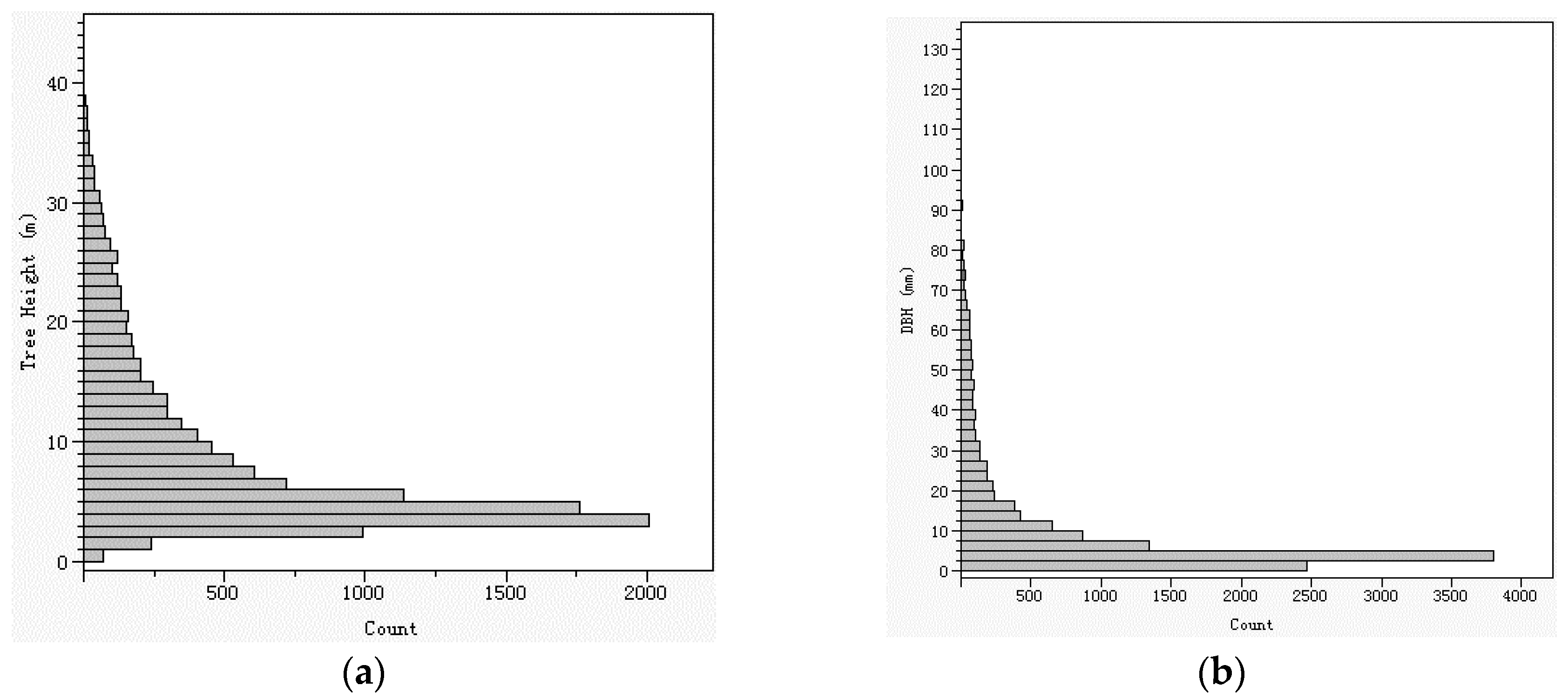
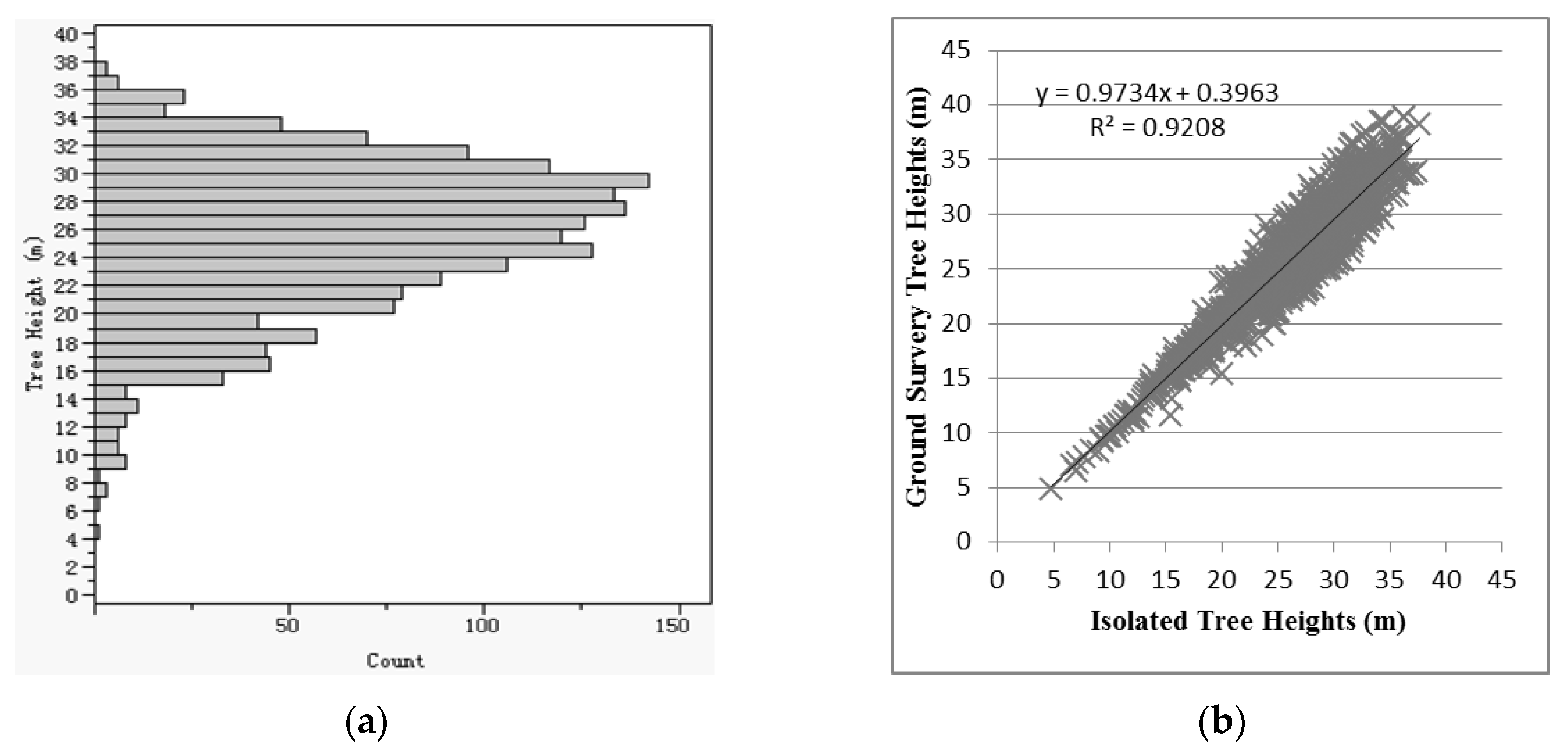
A mixed forest sample plot in the reserve was selected to test and validate our methods. The plot is a 300 × 300 m square that is divided into 900 small 10 × 10 m quadrats [36]. The ground survey was carried out between 23 July and 6 August 2009. Each individual tree with a DBH greater than 2 cm was marked with an aluminium plate. The species, DBH, tree height, and position of these trees were measured. DBH was measured using a diameter tape, tree height was measured using a laser altimeter, and position was measured using the distance from tree stem at breast height to the boundaries of the corresponding quadrat. The crown diameter was not measured. In total, 12,315 individual trees were recorded, and the tree height and DBH distributions are shown in Figure 1. Most trees were supressed small trees. The number of intermediate, co-dominant, and dominant trees formed a pyramid-like distribution, which meant the tree count was inversely proportional to the tree height.

Ground spectrum measurements were synchronized with the flight that acquired the hyperspectral data. The device used was a FieldSpec 3 Spectroradiometer (Malvern Panalytical, Egham, Surrey, UK) with a spectral range of 350 nm to 2500 nm, a spectral resolution of 3 nm at 700 nm and 10 nm at 1400/2100 nm, a sampling interval of 1.4 nm at 350 nm to 1050 nm and 2 nm at 1000 nm to 2500 nm, and a scanning interval of 0.1 second. Bright and dark objects and some typical ground objects were measured for the atmospheric correction of the hyperspectral image.

2.2. Acquiring Airborne Data and Pre-Processing

High-density airborne LiDAR data were acquired in August 2009. The LiDAR system was a LiteMapper 5600, which included a Riegl LMS-Q560 laser scanner and a DigiCAM charge coupled device (CCD) camera. LiteMapper 5600 provides full waveform analysis, which provide detailed vertical structure of forest. The parameters of LiteMapper 5600 are listed in

Table 1. Main technical parameters of LiteMapper 5600 system.

Device Type	LiteMapper 5600
Pulse repetition frequency	100 kHz
Laser wavelength	1550 nm
Pulse length	3.5 ns
Laser beam divergence	≤0.5 mrad
Multiple target separation within single shot	0.6 m
Return pulse width resolution	0.15 m
Scan pattern	Parallel scanning
Scan angle range	30°
Ground sample spot diameter	0.5 m (with flight height of 1000 m)

.

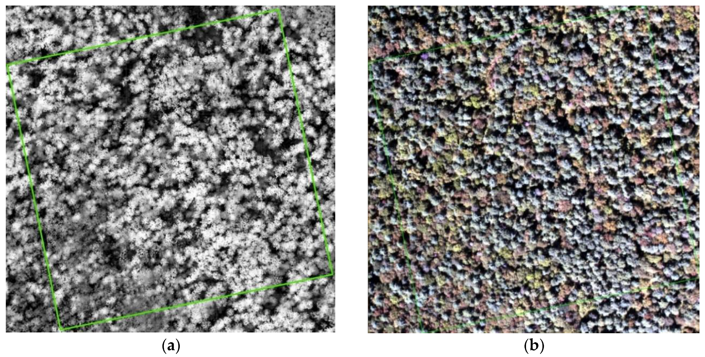
The flight covered an area of 100 km², with a flight height of 1022–1121 m, which was a relative flight height above the canopy of approximately 1000 m. A total of 12 flight strips with side overlaps of 90% were obtained. The point density was approximately 12 points/m². Point classification, digital surface model (DSM) generation, and digital elevation model (DEM) generation were conducted using the TerraScan software (TerraSolid, Helsinki, Finland). The canopy height model (CHM) (Figure 2a) was calculated using the difference between the DSM and the DEM at a resolution of 0.5 m. A digital orthographic map (DOM) with a resolution of 0.2 m was generated based on the CCD images and LiDAR-derived DEM using the TerraPhoto software (TerraSolid, Helsinki, Finland).

Hyperspectral data were also acquired in August 2009 using a CASI-1500 (Compact Airborne Spectrographic Imager) (Figure 2b) with the same flight height as the LiDAR flight. The time of acquisition was from 10:00 am to 14:00 pm, which was close to solar noon. CASI-1500 is a visible and near-infrared (VNIR) pushbroom sensor, and its optimal parameters are shown in

Table 2. Parameters of CASI-1500 images acquired in Liangshui.

Sensor Type	VNIR Pushbroom Sensor
Spectral Range	380–1050 nm
Spectral Channels	23
Spatial resolution	0.5 m
Field of View	40°
IFOV	0.49 mRad
Spectral Width	2.4 nm
Spectral Resolution	<3.5 nm
Bands (nm)	459.7, 533.6, 608.8, 693.6, 798.5, 817.5, 830.6, 834.2, 868.6, 880.5, 887.6, 913.7, 927.9, 955.1, 961.0, 982.2, 990.5, 997.6, 1002.3, 1011.7, 1015.2, 1032.9, 1039.9

. CASI-1500 allows the user to select either the spectral mode or spatial mode. The spectral mode provides up to 288 spectral bands, and the spatial mode, which was used in our experiment, provides a spatial resolution of 0.5 m, with a swath width of 1484 pixels and 23 spectral bands. First, radiometric and geometric corrections of raw CASI-1500 hyperspectral images were performed using Itres V1.2 (ITRES, Calgary, AB, Canada) which result in the radiance images with a ground sampling distance (GSD) of 1 m. Then, empirical line calibration (ELC) [37] was utilized for atmospheric correction to calibrate the radiances to the surface reflectance. After that, the ELC method assumes that a linear relationship exists between the radiance recorded by the sensor and the corresponding site-measured spectral reflectance, which requiring two or more bright and dark targets in the image coverage area. This study selected a flat and open ground to position two black and white pieces of cloth, with sizes of 5 m × 5 m (proportional to the pixel size of 0.5 m), to act as the dark and bright targets, respectively. The field spectra of the dark and bright targets were measured simultaneously.

3. Methods

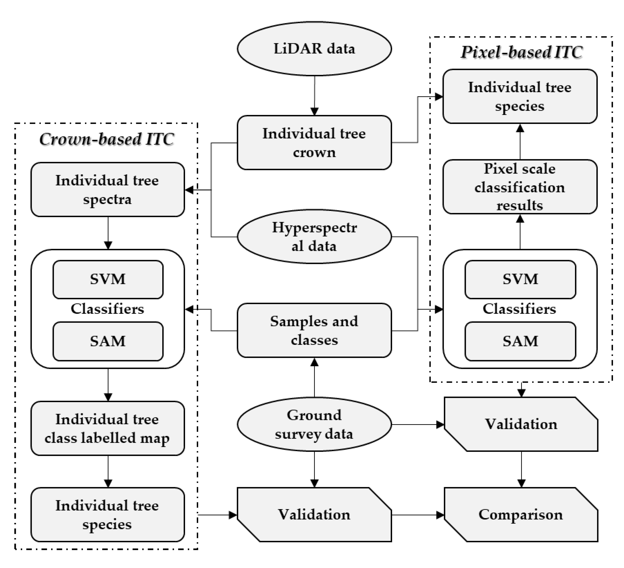
A flowchart of the method is summarized in Figure 3. Detailed information is given as follows:

3.1. Registration and Individual Tree Isolation

Registration was required because the hyperspectral data and LiDAR data were acquired separately. First, orthographic rectification was carried out based on the LiDAR-derived DEM to eliminate the image warping in the hyperspectral data caused by topographic relief [25,32,38,39]. Then, registration was executed by finding homonymous objects in the CHM, DOM, and hyperspectral data using the polynomial method in the ENVI software (Harris Geospatial Solutions, Inc., Boulder, CO, USA). The homonymous objects mainly included building corners, road intersections, and some small, clearly visible objects.

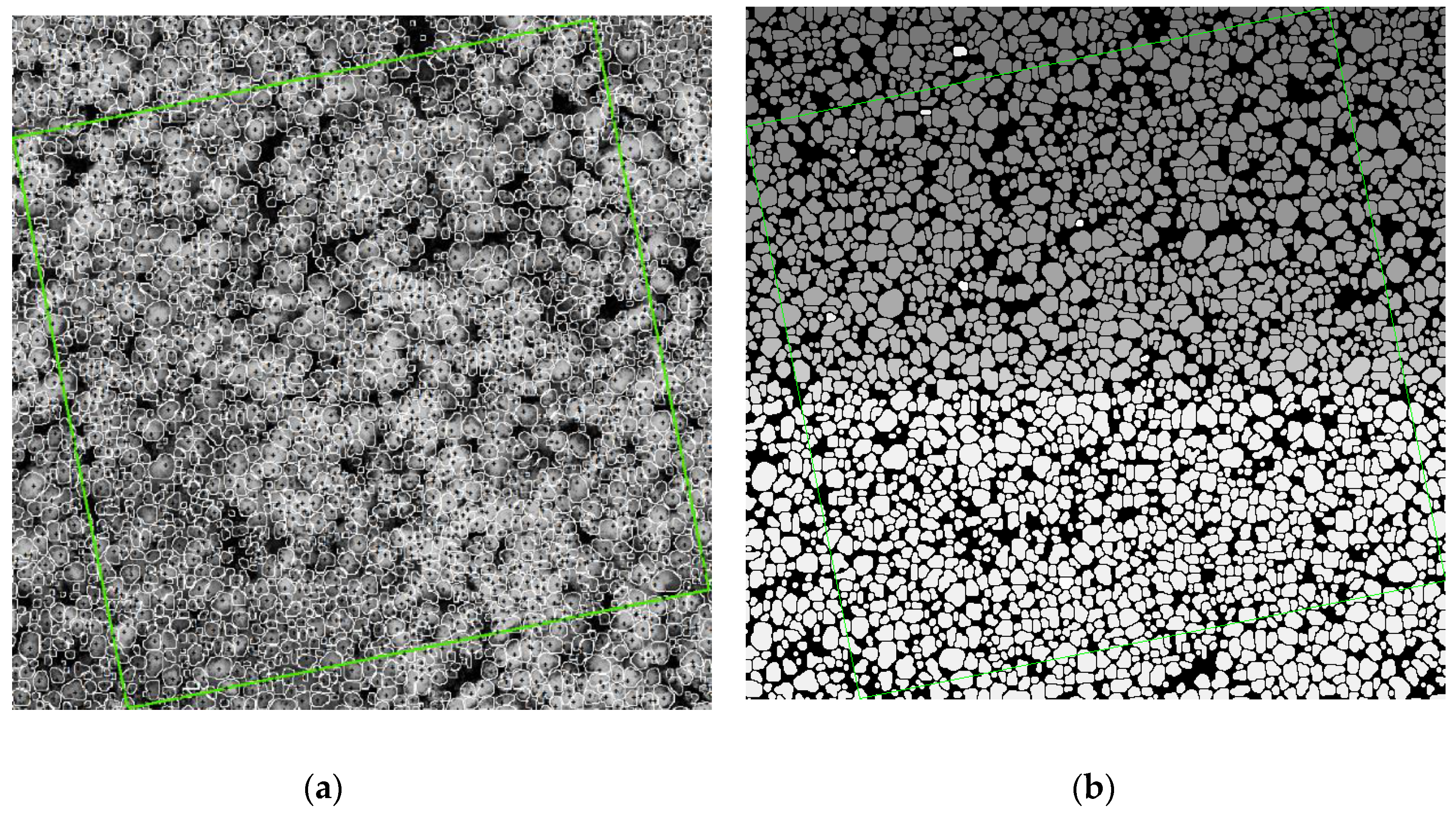
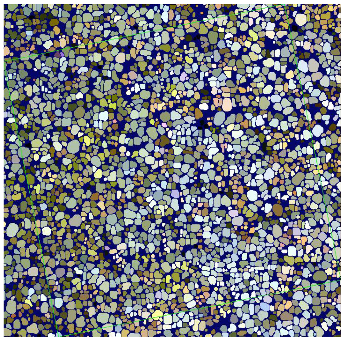
The individual trees were isolated in the CHM using a morphological crown control-based watershed algorithm, as proposed in our previous studies [18]. First, an invalid value filling method, which was also proposed in our previous studies, was applied to the original CHM to fill abnormal or sudden changes in the height values (i.e., invalid values) [38]. Then, the crown-controlled watershed method for individual tree isolation was applied to the CHM to obtain the position, height and crown diameter of individual trees. The morphological crown control, which approximates the real tree crown area in the CHM and is used to limit treetop detection and watershed operation in the crown area, was introduced to determine the crown areas. The local maxima algorithm identified potential individual tree positions. Double watershed transformations, in which a reconstruction operation was inserted, delineated the tree crowns. Finally, the individual trees were isolated, and their parameters were extracted from the optimized watershed results (Figure 4a). The green square in Figure 4a shows the plot boundary, the small black crosses represent individual tree positions, and the white boundaries are the individual tree crown edges. The labelled image (Figure 4b), in which each segment had its own label, was generated at the same time.

In total, 1847 individual trees were isolated from the plot, and the tree height distribution is shown in Figure 5a. 97.13% of the isolated trees are shown to have a tree height greater than 15 m. This situation is due to the CHM representing the upper surface of the canopy. The 2205 ground survey trees with height greater than 15 m were used to validate the results. Manual comparisons between the isolation results and the ground survey data were performed using the ArcGIS software. The validation principle is based on position proximity and tree height similarity [18]. After validation, 1838 trees were correctly isolated by finding its corresponding ground survey trees, and the comparison between LiDAR derived tree height and ground survey of the 1838 trees are shown in Figure 5b. The position, tree height, and species of the validated trees were recorded.

3.2. Classes Determination and Sample Selection

Individual tree spectra were extracted by searching for the corresponding spectrum pixels in the hyperspectral image based on the crown areas extracted from the individual tree isolation process (Equation (1)).

$$P_i=H\left(I_{W=i}\right)$$

(1)

where $P_i$ is hyperspectral pixels in basin $i$, $W$ is the label image of the watershed, $i$ is the unique label of a different basin, $H$ is the hyperspectral image, and $I_{W=i}$ is the index of label $i$ in $W$. In this step, the boundary pixels of each basin were not included, to avoid the possible mixture of crown to the background or another crown.

These pixels were merged to ensure that every tree is represented by one unique spectral curve, which is used to directly identify tree species. The label image of individual tree detection became a hyperspectral label image, that each label was marked by a mean spectral curve rather than the watershed label. For two reasons, not all the pixels located in the tree area were vegetation pixels. First, the registration accuracy between individual tree isolation results from LiDAR, and hyperspectral data did not reach 100% because of the different data acquisition times. Second, the four-component problem [26] resulted in shadow and ground pixels in the crown area. Thus, filtering should be carried out to eliminate the non-vegetation pixels before merging. The reflectance of healthy vegetation in the near-infrared and red bands is significantly different from the non-vegetation objects, according to the spectral reflection characteristics. Radiation in the green portion of the spectrum is strongly absorbed, whereas radiation in the near-infrared band is strongly reflected and penetrated [40]. Vegetation indices (e.g., normalized difference vegetation index, NDVI) are often used to determine whether a hyperspectral pixel is a vegetation pixel. The study area of the present paper is relatively small, and the main ground objects included only vegetation and the ground. Thus, an empirical threshold for the near-infrared band (798.5 nm) was used to directly distinguish vegetation from non-vegetation. As a result, the pixels with reflectance at 798.5 nm band greater than 0.1 were considered to calculate individual tree spectrum.

Spectrum merging was carried out by calculating the mean value of each band of the extracted individual tree crown pixels (Equation (2)). Figure 6 shows the merged individual tree spectra.

$$S_M=M(\overrightarrow{S_i})$$

(2)

where $\overrightarrow{S_i}$ is the vegetation spectral pixels of the individual tree $i$, $M()$ is the mean value calculation function, and $S_M$ is the mean spectrum.

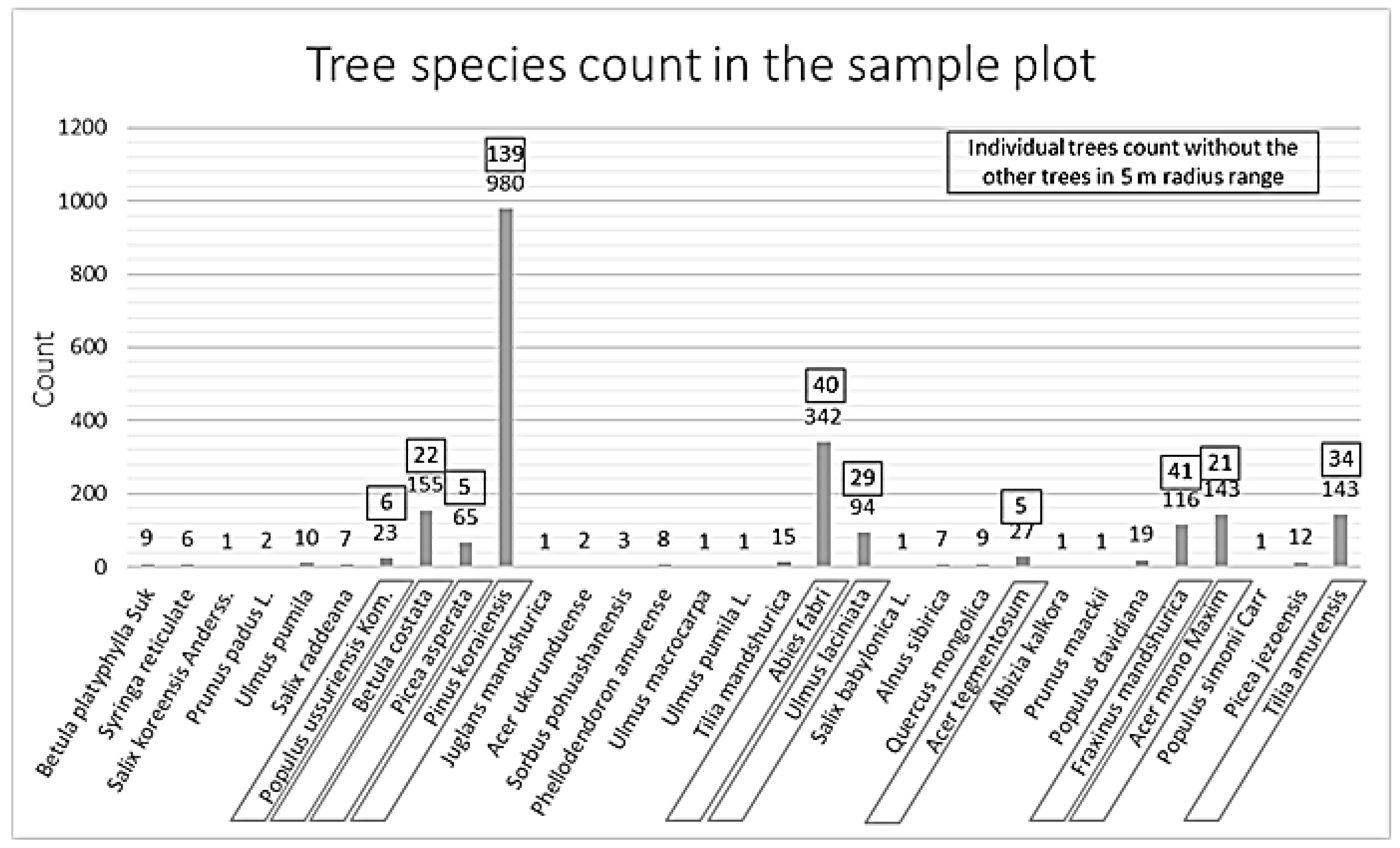
The CHM represents the canopy distribution of the upper surface of the forest, whereas the ground survey includes nearly all the individual trees in the sample plot. Thus, the ground survey data were filtered by tree height. Only trees with a height greater than 15 m were retained, as observed in the CHM. There were 31 species in total, of which four were needle leaved species and 27 were broadleaved species (Figure 7). To ensure the individual trees have pure crown spectrum, we only selected trees which did not have other trees around them in a range of 5 m radius. 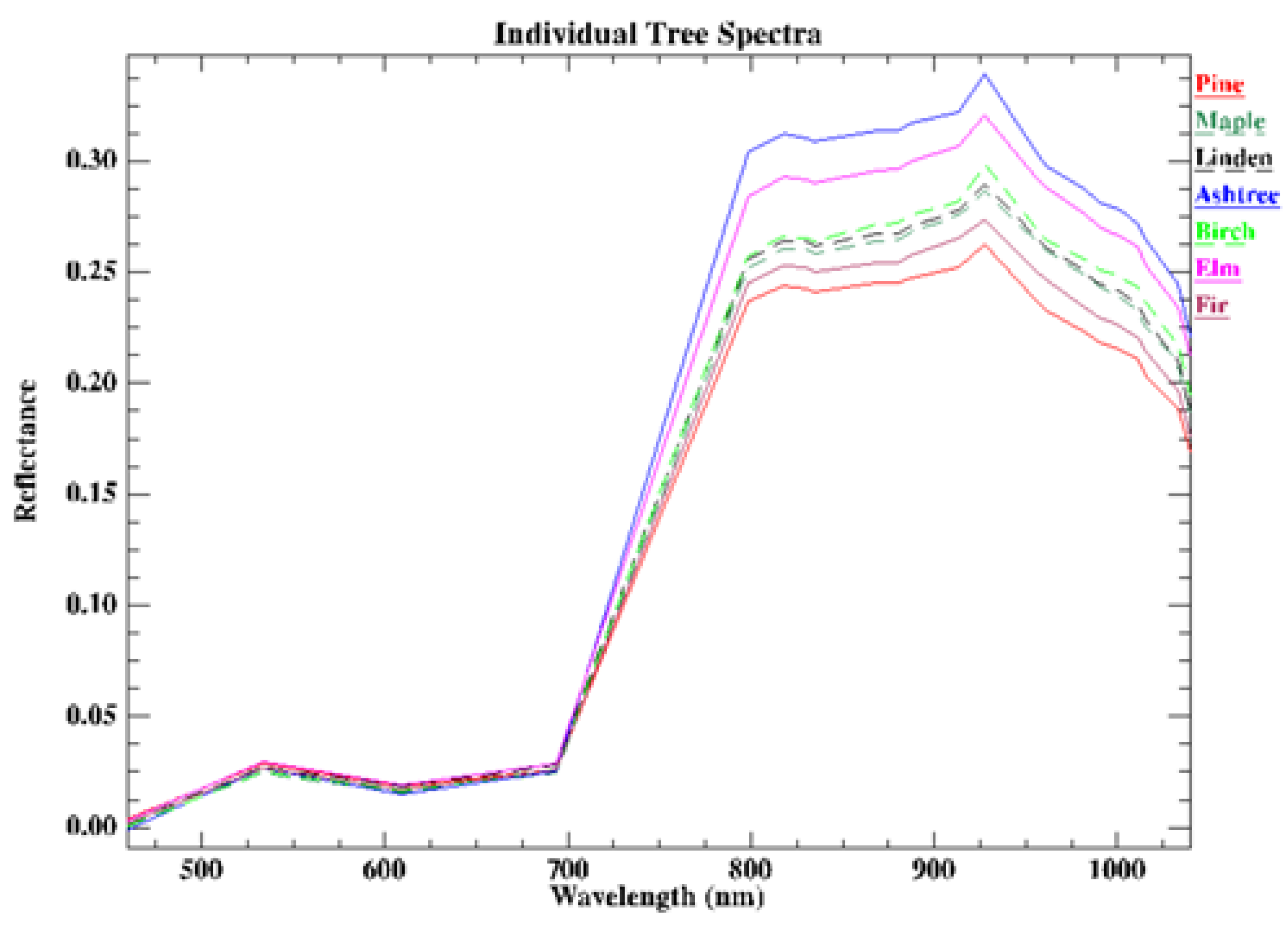The Figure 8 showed that Aspen, Spruce, and Maple did not have enough eligible samples. As a result, the Korean pine, Korean birch, Faber’s fir, Japanese elm, northeast China ash, acer mono, and amur linden were considered for individual tree spectrum extraction to determine classes system. We collected all spectra of the selected trees of the 7 species from Figure 7 based on the ground positions. Based on our previous work [40], it was difficult to identify species in the study area with single temporal spectra. As a result, the mean spectra of these species were checked and compared (Figure 8), the following observations were generated:

(1)

The spectrum of Korean pine was easily distinguished.

(2)

The spectra of Faber’s fir and dragon spruce were very similar.

(3)

The spectra of Korean birch, Acer mono and Amur linden were very similar.

(4)

The spectrum of northeast China ash was relatively unique.

(5)

The quantity of Japanese elm and the other broadleaved trees was small, and their spectra were roughly similar.

As a result, a total of 6 classes with species or species groups were defined to cover as much detail as possible:

(1)

A = Korean pine;

(2)

B = Faber’s fir and dragon spruce;

(3)

C = Korean birch, Acer mono and Amur linden;

(4)

D = northeast China ash;

(5)

E = Japanese elm, and the other broadleaved species;

(6)

Background.

Thirty samples per class were selected for classes A–E from the pure crown spectrum according their similarity to the average curve of each class, and another thirty samples were selected as the background. Each sample was an independent spectra curve, which provided a mean value for the vegetation pixels in a tree crown area.

3.3. Crown-Based ITC & Pixel-Based ITC

The crown-based ITC was then carried out with the 180 samples and spectra merged image in ENVI software. In this step, the classifiers, SVM and SAM [41,42], were trained by the samples, and then applied respectively to the spectra merged image. The classification results were classes labelled maps, in which each individual tree crown was labelled with a classified class, and then the species of each individual tree was obtained by extracting the unique class within its crown.

SVM is a classification system derived from statistical learning theory, which is very effective in the classification with limited samples. It separates the classes with a decision surface that maximizes the margin between the classes. The surface is often called the optimal hyperplane, and the data points closest to the hyperplane are called support vectors. The support vectors are the critical elements of the training set. SAM is a physically-based spectral classification that uses an n-dimensional angle to match pixels to reference spectra. The algorithm determines the spectral similarity between two spectra by calculating the angle between the spectra and treating them as vectors in a space with dimensionality equal to the number of bands.

In the pixel-based ITC, the same classifiers, SVM and SAM, were firstly applied to the original hyperspectral data with the same samples as used in crown-based ITC. The difference was that each sample was a spectral set of all crown pixels in the sample area, rather than one curve. Then, the individual tree isolation results were overlaid on the classification results. The class information for each isolated tree was extracted, and a weighted classes analysis method was applied to identify the class of the individual tree. In the weighted classes analysis, the weight of each pixel in an isolated tree crown was determined based on the distance between the pixel and the treetop, and the weight of the treetop pixel was 1, the farthest pixel was 0.5, while the other pixels were distributed linearly based on their distance to the treetop. Then, the weighted sum of each class was calculated, and the class with the largest sum was the class of the tree.

3.4. Validation & Analysing

The validation was carried out in two parts. First, 70% of the samples were randomly selected for classification training, and 30% were using for verification to provide overall accuracy (OA; the OA is calculated by summing the number of pixels classified correctly and dividing by the total number of pixels) and Kappa coefficient (KC; KC is calculated by multiplying the total number of pixels in all the ground truth classes (N) by the sum of the confusion matrix diagonals, subtracting the sum of the ground truth pixels in a class times the sum of the classified pixels in that class summed over all classes, and dividing by the total number of pixels squared minus the sum of the ground truth pixels in that class times the sum of the classified pixels in that class summed over all classes). Then, this procedure was repeated by 10 times to get a mean OA and KC.

After verification, the classification results were analysed by consistency between classification result and ground survey data. A buffer was established for each individual tree according to its extracted position and crown diameter. Individual trees identified in the ground survey that had a height greater than 15 m and that were located in the buffer, were compared with the classification results obtained from remote sensing data. If the class of the highest tree or the classes of the dominant trees with more than three individuals was the same as the classification result, then this tree would be considered correctly classified; otherwise, it was incorrectly classified. The consistency was defined as the ratio of correctly classified individual trees to the classified individual trees in each class.

Here, the buffer was imported to help find the corresponding ground survey trees rather than the crown delineated from the CHM. This was mainly because some of the trees in the plot were not vertical, which led to mismatches between the ground survey tree positions and the isolated tree positions. In this plot, the buffer was set to 1.5 times the crown diameter derived from the LiDAR data.

4. Results

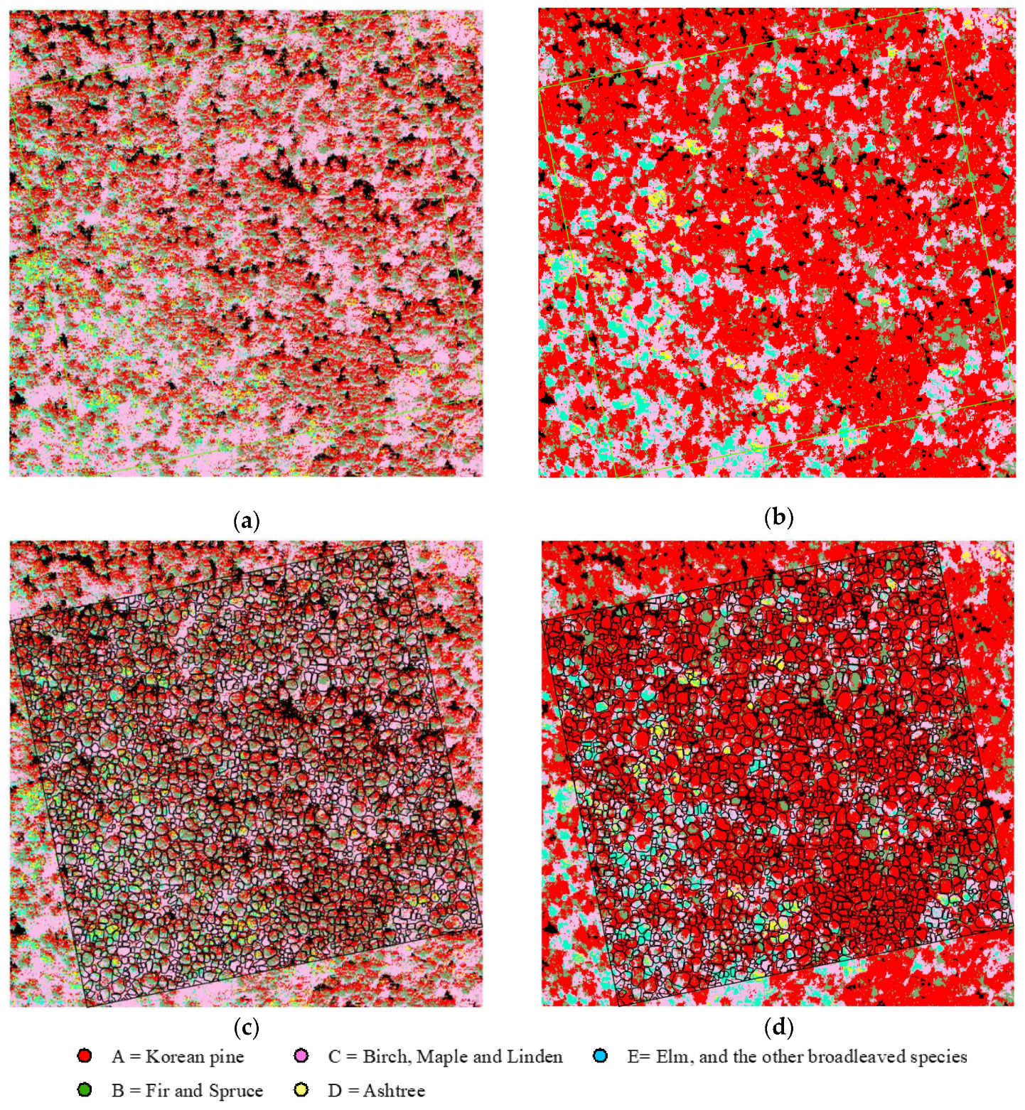
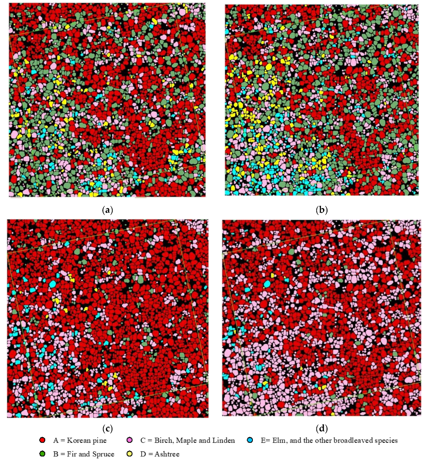
The hyperspectral image direct classification results of the SAM and SVM classifiers in ENVI software are shown in Figure 9a,b. Overlays of the individual tree isolation results on the classification results are shown in Figure 9c,d. The final classification results of the two methods are shown in Figure 10.

First, we used all samples for training to get results without validation. The individual tree classes statistics of the results without validation are shown in

Table 3. Classification result statistics (Count_Sur: Count of Survey data, Count_Exp: Count of Experiments, Percent in total: ratio of count to total, A–E are classes).

Class		A	B	C	D	E	Total
Survey Data (H > 15 m)	Count_Sur	980	419	313	125	368	2205
	Percent in total	44.44%	19.00%	14.20%	5.67%	16.69%	100.00%
Crown-based ITC SVM Results	Count_Exp	739	578	364	86	71	1838
	Percent in total	40.21%	31.45%	19.80%	4.68%	3.86%	100.00%
Crown-based ITC SAM Results	Count_Exp	531	561	419	126	195	1832
	Percent in total	29.22%	30.52%	22.80%	6.86%	10.61%	100.00%
Pixel-based ITC SVM Results	Count_Exp	1220	116	428	16	59	1839
	Percent in total	66.34%	6.31%	23.27%	0.87%	3.21%	100.00%
Pixel-based ITC SAM Results	Count_Exp	856	55	864	10	32	1817
	Percent in total	47.11%	3.03%	47.55%	0.55%	1.76%	100.00%

. From the table, the broadleaved classes appear too much in the pixel-based ITC results compared to the survey data. Generally, the classes distribution based on the crown-based ITC results is better than that of the pixel-based ITC. Each class generated the following observations:

(1)

Class A, in which the Korean pine was the dominant species in the plot, was frequently identified. The pixel-based ITC SVM method identified Class A with the highest frequency, the crown-based ITC SAM method identified it with the lowest frequency, and crown-based ITC SVM and crown-based ITC SAM identified it at nearly the same rate. The crown-based ITC methods obtained more Class A than the pixel-based ITC methods.

(2)

Class B, in which the Faber’s fir and dragon spruce were also the main dominant and sub-dominant species in the plot, was identified frequently using the pixel-based ITC method, whereas it was seldom identified using the crown-based ITC method.

(3)

Crown-based ITC identified Class C (Korean birch, Acer mono, and Amur linden) relatively close to the survey data, whereas pixel-based ITC SAM identified it more than 30%.

(4)

Class D (northeast China ash) was appropriately identified by crown-based ITC but just 1/8 identified by pixel-based ITC. This was mainly because crown-based ITC reduced the influence of the crown overlap.

(5)

The tree heights of the Japanese elm and the other broadleaved species in Class E were relatively low. Therefore, they were only partially identified by both pixel-based ITC and crown-based ITC.

(6)

Several trees were classified as background, which resulted in five tree classes with fewer than 1847 trees classified in each method.

From the observations, pixel-based ITC SVM was failed to distinguish class A and B, while SAM was failed to class B and C. These indicated that the results of pixel-based ITC were obviously not matching the ground survey data well. Therefore, the validation was only carried out on the crown-based ITC results.

The validation was carried out, and the OA and KC of each repeat for crown-based ITC SVM and crown-based ITC SAM were showed in

Table 4. Validation result statistics for crown-based ITC.

Repeat	Crown-Based ITC SVM		Crown-Based ITC SAM
	OA	Kappa	OA	Kappa
1	93.33%	89.36%	86.67%	81.23%
2	88.67%	82.61%	85.33%	79.20%
3	85.33%	81.45%	88.67%	82.58%
4	82.67%	80.22%	80.67%	74.22%
5	90.67%	87.34%	88.00%	85.44%
6	79.33%	73.28%	73.33%	69.88%
7	84.67%	79.28%	86.67%	81.19%
8	92.67%	88.76%	78.67%	70.94%
9	72.67%	67.55%	66.67%	56.82%
10	83.33%	79.46%	82.00%	73.74%
Mean	85.33%	80.93%	81.67%	75.52%

. The mean OA and KC of SVM were 85.33% and 80.93%, and SAM were 81.67% and 75.52%. Both the mean OA and KC of SVM were better than SAM.

The consistency with the field measurements (

Table 5. Consistency result statistics for crown-based ITC (Count_Sur: Count of Survey data, Count_Exp: Count of Experiments, Percent in total: ratio of count to total, A–E are classes).

Class		A	B	C	D	E	Total
Survey Data (H > 15 m)	Count_Sur	980	419	313	125	368	2205
	Percent in total	44.44%	19.00%	14.20%	5.67%	16.69%	100.00%
Crown-based ITC SVM Results	Count_Exp	739	578	364	86	71	1838
	Percent in total	40.21%	31.45%	19.80%	4.68%	3.86%	100.00%
	Correct count	701	334	230	42	58	1365
	Consistency	94.86%	57.79%	63.19%	48.84%	81.69%	74.27%
	Ratio to survey data	71.53%	79.71%	73.48%	33.60%	15.76%	61.90%
Crown-based ITC SAM Results	Count_Exp	531	561	419	126	195	1832
	Percent in total	28.98%	30.62%	22.87%	6.88%	10.64%	100.00%
	Correct count	514	375	283	79	141	1392
	Consistency	96.80%	66.84%	67.54%	62.70%	72.31%	75.98%
	Ratio to survey data	52.45%	89.50%	90.42%	63.20%	38.32%	63.13%

) also showed the similar results to the validation. From the table, Class A, the dominant species, has the highest consistency; both SVM and SAM have a consistency of approximately 95%. The consistencies of Classes B and C are approximately 60%, whereas the consistency of Class D using SAM is higher than that obtained using SVM, and the consistency of Class E is opposite with respect to SAM and SVM. The overall consistencies of SVM and SAM are not significantly different, and the identification consistency of each class should be considered to help assess the methods.

The sample plot is a mixed forest, in which Classes A and B have higher tree height. Based on the statistics of trees with a tree height greater than 15 m, the average tree heights of Classes A, B, and C, are 24.7 m, 20.18 m, and 19.9 m, respectively, and the average tree height of Classes D and E is 19 m. Based on the principle of individual tree isolation [18], Classes A, B, and C should be more isolated due to their greater height. Additionally, the hyperspectral image is “viewing the crown from above”, which leads to species with greater tree heights being identified more frequently. As shown in Table 3 and Table 4, the SVM results are consistent with the fact that the greater height classes outnumbered the other classes.

Finally, we analysed the classification errors in the crown-based ITC SVM results based on the buffer analysing (

Table 6. The confusion matrices of buffer based analyzing for crown-based ITC SVM (Count_Exp: Count of Experiments, A–E are classes).

Class	A	B	C	D	E	Total
Count_Exp	739	578	364	86	71	1838
A	701	20	9	4	5	739
B	182	334	34	24	4	578
C	84	33	230	7	10	364
D	12	10	18	42	4	86
E	3	5	3	2	58	71
Total	982	402	294	79	81	1838

). From the table, the OA and KC were 74.27% and 62.11%. Classes A and B were likely to be mutually misclassified because the spectra of these two coniferous species are similar. Overlapping tree crowns were another cause of the above problem. The method can eliminate some of the non-vegetation pixels in the crown area but could not distinguish the overlapping crown pixels. Thus, the merged spectra may mix spectra of two or more trees. In fact, misclassification is impossible to avoid because the plot is a high-density mixed forest. Additionally, incorrect validation can also be caused by the misregistration between individual tree isolation results and ground survey data. The trees in our plot are not all perfectly vertical. If the tree grows at an angle, the crown centre, which is considered the tree position in individual tree isolation, is located at a certain distance from the real tree position.

5. Discussion

Individual tree classification based on LiDAR and hyperspectral data from forests is a method that could save a considerable amount of time, manpower, and material resources during forest investigations. This research verifies that the mean spectra of the crown could represent individual tree spectra and it is more suitable for the individual tree species identification than pixel-based classification. Based on experiments, our approach and data appear to be suitable for the isolation and classification of dominant and sub-dominant individual trees and can be applied to forests with simple vertical structures, such as a planted forest. There were some advantages and limitations in the use of this approach. Classification based on hyperspectral data usually encounters several problems, e.g., mixed-pixel and four-component problems. The pixel-based ITC methods first executed classification and then analysed individual tree classes based on the individual tree isolation results. Thus, these problems still existed when executing pixel-based classification. To overcome these problems, the crown-based ITC methods used a merged spectrum, which involved merging the spectra of one tree into a single spectrum, to avoid the mixed-pixel problem at the level of individual tree and, in doing so, largely weakened the four-component problem by neutralizing the components. However, this largely depends on the registration accuracy of the hyperspectral and LiDAR-derived CHM. The registration directly determines the purity of the individual spectra. The registration in this study was executed by finding homonymous objects around the plot. However, a mass of homonymous objects would be required to ensure an accurate registration when applying our method to large areas, it would be more feasible to use object-based registration, which isolates individual trees in both hyperspectral and CHM images and then registers the images based on the homonymous or most similar individual tree group [43].

The crown-based ITC method extracted an individual tree spectrum from a hyperspectral image based on the label image obtained from the isolation using the LiDAR CHM. A threshold was defined to eliminate non-vegetation pixels, and the vegetation pixels were then merged by calculating the mean value of spectra. Then, every individual crown had its own spectral curve. Zhang et al. [27] used the spectrum of the treetop pixel to represent an individual tree spectrum, which was appropriate because the trees in an urban area had a relatively regular shape and little overlap. Dalponte et al. [29] used thresholds to extract hyperspectral pixels inside individual tree crowns from individual tree isolation models based on LiDAR or hyperspectral images to ensure that the pixels were the real crown surface. All these vegetation pixels were then used in the classification. However, this approach still encounters the problems of mixed-pixels, four-component, and overlapping crowns. As a result, merging the crown pixels would be better for identifying individual tree species. The results of the individual tree species identification had a good relationship with tree height. A taller tree was more likely to be correctly identified, and smaller trees and understories were difficult to detect. The results also indicated that greater consistency was obtained with dominant and sub-dominant species compared to other species. The reason for this could be that both the LiDAR CHM and hyperspectral data represented the upper surface of the crown. Although LiDAR had some penetration ability, the individual tree isolation process was carried out based only on the CHM. The dominant and sub-dominant species groups were better observed in images, whereas the midstory and understory species groups were mostly overlapping. The validation results of individual isolation had the same pattern as the results of Zhao et al. [18], which showed that the LiDAR CHM- based individual tree isolation could provide good information about the dominant and sub-dominant trees in forests. Thus, dominant and sub-dominant species were set to individual classes, and other species were grouped when determining classes.

The mean OA and KC of this study for crown-based ITC SVM were 85.33% and 80.93%. According to

Table 7. The overall accuracy comparison of some individual tree species classification studies.

Methods/Literature	Classes	Overall Accuracy	Location
crown-based ITC SVM	6	85.33%	Temperate forest in China
Maschler et al. 2018	13	89.4%	Temperate forest in Australia
Dalponte et al. 2019	9	88.1%	Temperate forest in US
Nevalainen et al. 2017	4	>90%	Boreal forest in Southern Finland
Zhang et al. 2012	20	68.8%	Urban forest in north Dellas
Alonzo et al. 2014	29	83.4%	Urban forest in California
Lee et al. 2016	7	>85%	Deciduous forest in England

, our results confirmed that the overall accuracy of individual tree species classification based on LiDAR and hyperspectral data could achieve around 85%. The classes of this study were limited, and larger study area should be considered for further research. The classification errors were mainly attributable to similar spectra, crown overlap, and registration between isolation results and ground survey data. In future studies, the latter two problems can be remedied, or even avoided. Crown overlap always leads to over- or under-isolation, and this issue is frequently encountered in individual tree isolation studies. A 3D structural individual tree isolation process based on a high-density point cloud could be studied to reduce over- and under-isolation. For the registration between isolation results and ground survey data, a potential solution is to replace individual positions with the individual treetops in the field works, which will be more suitable for remote sensing-based individual tree applications.

The six classes used in this paper are defined based on hyperspectral image, and classes B, C and E are actually “mixed genera”. This is likely because that the hyperspectral data we used just has 23 bands, which are insufficient to distinguish some spectra-similar species, such as the species in classes B and C. In future, we are intending to realize “real species” classification in a large region with more samples and the hyperspectral data with more detail bands. The classifiers used were SVM and SAM, which are frequently used in hyperspectral image classification. Some of the latest algorithms, such as adaptive Gaussian fuzzy learning vector quantization, may be better methods [27].

A significant limitation of this research is the combination of LiDAR and hyperspectral data. Airborne LiDAR and hyperspectral data acquisition are still expensive because individual-scale parameter extraction requires high-density point clouds and high-resolution hyperspectral data, as well as synchronous data acquisitions. However, the expense will decrease in the future as technology continues to improve. For example, an integrated device, like the LiCHy-CAF, which can combine the two flights into one by integrating LiDAR and hyperspectral sensors, as well as the development of systems to acquire LiDAR and hyperspectral imagery from UAVs will significantly reduce the cost.

6. Conclusions

Individual tree information in forest, including position, height, and species, could be extract based LiDAR and hyperspectral data, especially for the dominant and sub-dominant trees. Two individual tree classification methods, namely crown-based ITC and pixel-based ITC, based on LiDAR and hyperspectral data, were proposed and compared in this paper. The results in Northeast China showed that the crown-based ITC method performed better than the pixel-based ITC method. It could be concluded that the individual tree species should be classified based on individual tree crown-based spectrum features, rather than analyzed based on pixel-based classification results using individual crowns.

Following crown-based ITC method, the identification consistency of the class of the dominant species relative to the field measurements was greater than 90%, whereas that of the classes of the sub-dominant species groups were greater than 60%. The overall consistencies of SVM and SAM were both greater than 70%, but SVM reflected the species distribution of the experiment area better than SAM. It also could be concluded that individual tree species classification based on LiDAR and hyperspectral data can be applied to distinguish dominant and sub-dominant species in forests with high accuracy, but remains powerless in the case of non-dominant species.